Load Cell Design Using COMSOL Multiphysics

Andrei Marchidan, Tarah N. Sullivan and Joseph L. PalladinoDepartment of Engineering, Trinity College, Hartford, CT 06106, USA

joseph.palladino@trincoll.edu

Abstract— COMSOL Multiphysics was used todesign a binocular load cell. A three-dimensionallinear solid model of the load cell spring elementwas studied to quantify the high-strain regions underloading conditions. The load cell was fabricated from6061 aluminum, and general purpose Constantin al-loy strain gages were installed at the four high-strainregions of the spring element. The four gages werewired as a full Wheatstone bridge configuration andtotal strain was measured for applied loads rangingfrom 0-2.5 kg in 100 g increments. Model total strainwas measured using point probes at each of the fourstrain locations, and with a load parametric analysis.Absolute mean model-predicted strain was 1.41% ofmeasured strain. The load cell was highly linear, withcorrelation coefficient r2=0.9999.

Keywords: load cell, COMSOL Multiphysics,solid mechanics, strain gage, force transducer.

I. INTRODUCTION

LOAD cells are commonly used force trans-ducers that convert an applied mechanical

load into a voltage. Load cells typically comprisespring elements that are designed to deform withload, strain gages that vary their resistance withdeformation (strain) of the spring element, and aWheatstone bridge circuit that produces voltageproportional to strain. One popular spring elementdesign is the binocular configuration, which is abeam with two holes and a web of beam materialremoved, as shown in Figure 1. The complexityof the binocular section of this beam preventsprediction of strain via simple hand calculation;hence, a COMSOL model was used to guide loadcell design.

II. METHODS

1) Equations: Modeling the load cell requiresthree equations: an equilibrium balance, a con-stitutive relation relating stress and strain, and a

Fig. 1. Load cell spring element with “binocular” design.

kinematic relation relating displacement to strain.Newton’s second law serves as the equilibriumequation, which in tensor form is:

∇ · σ + Fv = ρ u (1)

where σ is stress, Fv is body force per volume, ρis density, and u is acceleration. For static analysis,the right-hand side of this equation goes to zero.

The constitutive equation relating the stress ten-sor σ to strain ε is the generalized Hooke’s law

σ = C : ε (2)

where C is the fourth-order elasticity tensor and: denotes the double dot tensor product. In COM-SOL, this relation is expanded to

σ − σ0 = C : (ε − ε0 − εinel) (3)

For this application, initial stress σ0, initial strainε0, and inelastic strain εinel are all zero. Forisotropic material, the elasticity tensor reduces to

Excerpt from the Proceedings of the 2012 COMSOL Conference in Boston

the 6X6 elasticity matrix:

2µ + λ λ λ 0 0 0λ 2µ + λ λ 0 0 0λ λ 2µ + λ 0 0 00 0 0 µ 0 00 0 0 0 µ 00 0 0 0 0 µ

(4)

where λ and µ are the Lame constants

λ =E ν

(1 + ν)(1 − 2ν)and µ =

E

2(1 + ν).

E is elastic modulus and ν is Poisson’s ratio, withmaterial properties listed in Table I.

The final required equation is the kinematicrelation between displacements u and strains ε. Intensor form

ε =12

[∇u + (∇u)T

](5)

where T denotes the tensor transpose. For rectan-gular Cartesian coordinates the strain tensor maybe written in indicial notation [3]

εij =12

[∂uj

∂xi+

∂ui

∂xj− ∂uα

∂xi

∂uα

∂xj

](6)

where α=1,2,3,. . . . For small deformations thehigher order terms are negligible and εij reducesto Cauchy’s infinitesimal strain tensor:

εij =12

[∂uj

∂xi+

∂ui

∂xj

](7)

TABLE IMATERIAL PROPERTIES FOR 6061 ALUMINUM USED IN THE

COMSOL MODEL [2].

Parameter Symbol Value

Elastic Modulus E 69 GPaPoisson’s Ratio ν 0.33Density ρ 2700 kg/m3

2) COMSOL Multiphysics Model: A 3D solidmechanics model was built, with geometry drawnin SolidWorks (Figure 6) and imported using theCOMSOL CAD Import Module. The spring ele-ment was modeled as homogeneous, linearly elastic6061 aluminum. The left-hand end of this beamwas defined as a fixed constraint boundary. Loads

were applied to the right-hand end of the beam asa point load in the y direction.

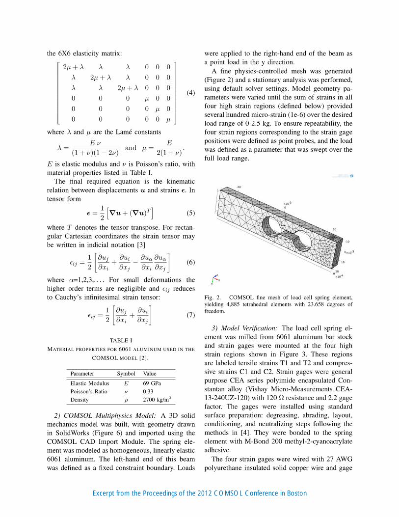
A fine physics-controlled mesh was generated(Figure 2) and a stationary analysis was performed,using default solver settings. Model geometry pa-rameters were varied until the sum of strains in allfour high strain regions (defined below) providedseveral hundred micro-strain (1e-6) over the desiredload range of 0-2.5 kg. To ensure repeatability, thefour strain regions corresponding to the strain gagepositions were defined as point probes, and the loadwas defined as a parameter that was swept over thefull load range.

Fig. 2. COMSOL fine mesh of load cell spring element,yielding 4,885 tetrahedral elements with 23.658 degrees offreedom.

3) Model Verification: The load cell spring el-ement was milled from 6061 aluminum bar stockand strain gages were mounted at the four highstrain regions shown in Figure 3. These regionsare labeled tensile strains T1 and T2 and compres-sive strains C1 and C2. Strain gages were generalpurpose CEA series polyimide encapsulated Con-stantan alloy (Vishay Micro-Measurements CEA-13-240UZ-120) with 120 Ω resistance and 2.2 gagefactor. The gages were installed using standardsurface preparation: degreasing, abrading, layout,conditioning, and neutralizing steps following themethods in [4]. They were bonded to the springelement with M-Bond 200 methyl-2-cyanoacrylateadhesive.

The four strain gages were wired with 27 AWGpolyurethane insulated solid copper wire and gage

Excerpt from the Proceedings of the 2012 COMSOL Conference in Boston

T1 C1

C2 T2

Fig. 3. Location of transducer spring element high strainregions T1, C1, T2., and C2.

lead wires were kept of uniform length to pre-vent unwanted lead resistance differences. The fourgages were wired as a full bridge (FB 4 active)using four conductor shielded cable and connectedto a bridge amplifier (Vishay P3 Strain Indicatorand Recorder [5]). Figure 4 shows the full bridgelayout with two opposite legs in tension and theother two in compression. Total strain is then givenby

εtotal = εT1 − εC1 + εT2 − εC2 (8)

When loaded, the bridge output is linearly propor-tional to the load. The bridge amplifier providesthe excitation voltage Vi and, after the bridge isbalanced and the gage factor is input, produces anoutput voltage Vo directly in units of micro-strain.

III. RESULTS

Figure 5 shows bending strain arising from anapplied load of 1 kg. The highly scaled deformationimage shows how the four high strain regionscorrespond to simultaneous tension in the T1 andT2 regions and compression in the C1 and C2regions. Plotted is the strain tensor x-component.Table II lists strain corresponding to the locationsof each of the four strain gages for each appliedmass. Also shown is total model strain, computedusing equation 8 in microstrain, labeled COMSOL.The next table column lists measured transducerstrain, and the last column shows percent differencebetween model total strain and measured totalstrain. The absolute mean percent difference was

Fig. 4. Full bridge configuration of the four strain gagesshowing one pair of tensile and one pair of compressive strains.P+, P-, S+, and S- refer to P2 bridge amplifier connections.

1.4%. Figure 7 is a plot of measured total strainas a function of applied load. The load cell is verylinear, with correlation coefficient of 0.9999.

2.5 1 1.5 2

600

150

200

250

300

350

400

450

500

550

Applied Load [kg]

Load

Cel

l Tot

al S

trai

n [e

-6] y = 232x + 3.277 R² = 0.9999

Fig. 7. Measured total strain of completed transducer for loadrange 0-2.5 kg, showing high degree of linearity.

IV. DISCUSSION AND CONCLUSIONS

Load cell design is challenging due to the com-plex geometry of spring elements. COMSOL solidmodels are useful for predicting strain in thesedesigns, for locating strain gage mounting positionsand especially for optimizing maximum strain forthe desired load range. Model predictions werevalidated by measurements performed with the

Excerpt from the Proceedings of the 2012 COMSOL Conference in Boston

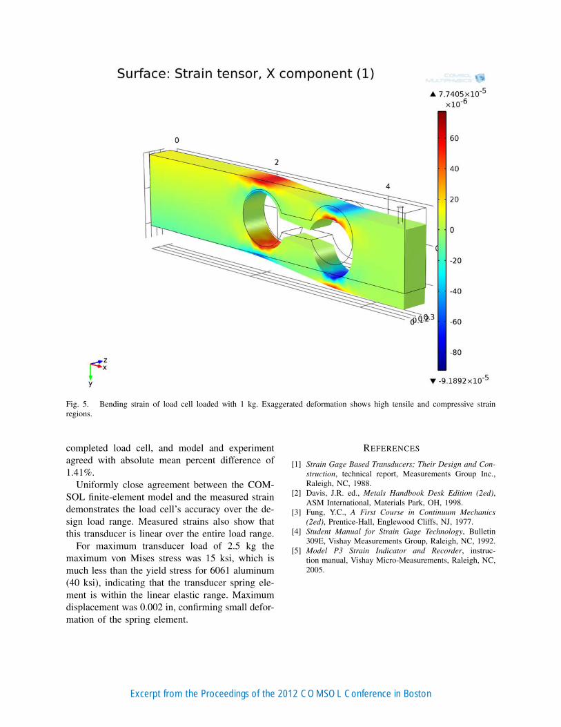
Fig. 5. Bending strain of load cell loaded with 1 kg. Exaggerated deformation shows high tensile and compressive strainregions.

completed load cell, and model and experimentagreed with absolute mean percent difference of1.41%.

Uniformly close agreement between the COM-SOL finite-element model and the measured straindemonstrates the load cell’s accuracy over the de-sign load range. Measured strains also show thatthis transducer is linear over the entire load range.

For maximum transducer load of 2.5 kg themaximum von Mises stress was 15 ksi, which ismuch less than the yield stress for 6061 aluminum(40 ksi), indicating that the transducer spring ele-ment is within the linear elastic range. Maximumdisplacement was 0.002 in, confirming small defor-mation of the spring element.

REFERENCES

[1] Strain Gage Based Transducers; Their Design and Con-struction, technical report, Measurements Group Inc.,Raleigh, NC, 1988.

[2] Davis, J.R. ed., Metals Handbook Desk Edition (2ed),ASM International, Materials Park, OH, 1998.

[3] Fung, Y.C., A First Course in Continuum Mechanics(2ed), Prentice-Hall, Englewood Cliffs, NJ, 1977.

[4] Student Manual for Strain Gage Technology, Bulletin309E, Vishay Measurements Group, Raleigh, NC, 1992.

[5] Model P3 Strain Indicator and Recorder, instruc-tion manual, Vishay Micro-Measurements, Raleigh, NC,2005.

Excerpt from the Proceedings of the 2012 COMSOL Conference in Boston

TABLE IICOMSOL MODEL STRAINS T1, C1, T2 AND C2, RESULTING MODEL TOTAL STRAIN, MEASURED TOTAL STRAIN, AND

PERCENT DIFFERENCE FOR ALL APPLIED LOADS.

Mass T1 C1 T2 C2 COMSOL Measured Difference[g] [ε] [ε] [ε] [ε] [µε] [µε] [%]

500 3.24E-05 -2.71E-05 2.69E-05 -3.26E-05 119 120 0.840600 3.89E-05 -3.25E-05 3.23E-05 -3.92E-05 143 144 0.770700 4.54E-05 -3.80E-05 3.76E-05 -4.57E-05 167 167 0.180800 5.19E-05 -4.34E-05 4.30E-05 -5.22E-05 191 190 -0.262900 5.84E-05 -4.88E-05 4.84E-05 -5.88E-05 214 214 -0.187

1,000 6.49E-05 -5.42E-05 5.38E-05 -6.53E-05 238 233 -2.1831,100 7.14E-05 -5.96E-05 5.92E-05 -7.18E-05 262 257 -1.9081,200 7.78E-05 -6.51E-05 6.45E-05 -7.83E-05 286 280 -1.9951,300 8.43E-05 -7.05E-05 6.99E-05 -8.49E-05 310 304 -1.8091,400 9.08E-05 -7.59E-05 7.53E-05 -9.14E-05 333 327 -1.9201,500 9.73E-05 -8.13E-05 8.07E-05 -9.79E-05 357 350 -2.0161,600 1.04E-04 -8.68E-05 8.60E-05 -1.04E-04 381 373 -2.0481,700 1.10E-04 -9.22E-05 9.14E-05 -1.11E-04 405 397 -1.8781,800 1.17E-04 -9.76E-05 9.68E-05 -1.18E-04 429 420 -2.1891,900 1.23E-04 -1.03E-04 1.02E-04 -1.24E-04 452 445 -1.5492,000 1.30E-04 -1.08E-04 1.08E-04 -1.31E-04 477 468 -1.8872,100 1.36E-04 -1.14E-04 1.13E-04 -1.37E-04 500 491 -1.8002,200 1.43E-04 -1.19E-04 1.18E-04 -1.44E-04 524 514 -1.9082,300 1.49E-04 -1.25E-04 1.24E-04 -1.50E-04 548 537 -2.0072,400 1.56E-04 -1.30E-04 1.29E-04 -1.57E-04 572 561 -1.9232,500 1.62E-04 -1.36E-04 1.34E-04 -1.63E-04 595 584 -1.849

Absolute Mean % Difference 1.41

Excerpt from the Proceedings of the 2012 COMSOL Conference in Boston

Fig. 6. Load cell geometry drawn in SolidWorks, then imported into COMSOL with CAD Import Module. The small hole atthe right-hand end allows for suspending weights.

Excerpt from the Proceedings of the 2012 COMSOL Conference in Boston