load and resistance factor design of shallow

LOAD AND RESISTANCE FACTOR DESIGN OF SHALLOW

FOUNDATIONS FOR

BRIDGESbv

Jou·Jun Robert Chen

Dr. Kamal B. Rojiani, Chairman

Civil Engineering

(ABSTRACT) ·

Load Factor Design (LFD), adopted by AASHTO in the mid-1970, is currently used for

bridge superstructure design. However, the AASHTO specifications do not have any

LFD provisions for foundations. In this study, a LFD format for the design of shallow

foundations for bridges is developed.

Design equations for reliability analysis are formulated. Uncertainties in design pa-

rameters for ultimate and serviceability limit states are evaluated. A random field

model is employed to investigate the combined inherent spatial variability and sys-

tematic error for serviceability limit state. Advanced first order second moment

method is then used to compute reliability indices inherent in the current AASHTO

specifications. Reliability indices for ultimate and serviceability limit states with dif-

ferent safety factors and dead to live load ratios are investigated. Reliability indices

for ultimate limit state are found to be in the range of 2.3 to 3.4, for safety factors be-

tween 2 and 3. This is shown to be in good agreement with l\/leyerhof’s conclusion

(1970). Reliability indices for serviceability limit state are found to be in the range of

0.43 to 1.40, for ratios of allowable to actual settlement between 1.0 to 2.0. This ap-

II

pears to be in good agreement with what may be expected. Performance factors are Ithen determined using target reliability indices selected on the basis of existing risklevels.

I

Table of Centents

INTRODUCTION ......................................................... 11.1 GENERAL.......................................................... 11.2 OBJECTIVE AND SCOPE 21.3 ORGANIZATION ..................................................... 2

LITERATURE REVIEW .................................................... 4

2.1 GENERAL .......................................................... 4

2.2 CURRENT PRACTICE FOR SHALLOW FOUNDATION DESIGN ................... 52.3 LIMIT STATES AND UNCERTAINTIES IN SHALLOW FOUNDATION DESIGN ........ 17

2.4 REL|ABILITY·BASED DESIGN .......................................... 20

UNCERTAINTY ANALYSIS FOR ULTIMATE LIMIT STATE ......................... 27

3.1 GENERAL......................................................... 273.2 MODEL FOR ULTIMATE BEARING CAPACITY PREDICTION ................... 28

3.3 UNCERTAINTY ANALYSIS ............................................ 31

3.4 UNCERTAINTY FROM SOIL PARAMETER ................................. 40

3.5 SUMMARY OF UNCERTAINTIES IN BEARING CAPACITY PREDICTION ........... 44

Table of Ccntents v

I

UNCERTAINTY ANALYSIS FOR SERVICEABILITY LIMIT STATE .................... 464.1 GENERAL ......................................................... 464.2 MODEL FOR SERVICEABILITY LIMIT STATE ............................... 474.3 MODEL UNCERTAINTY ............................................... 504.4 INHERENT SPATIAL VARIABILITY AND SYSTEMATIC ERROR ................. 51

4.4.1 Equivalent Random Variable Model .................................. 54

4.4.2 Evaluation of Ni and NS ........................................... 594.5 SUMMARY OF UNCERTAINTIES FOR SETTLEMENT ANALYSIS................. 63

STATISTICS OF LOADS .................................................. 665.1 GENERAL......................................................... 665.2 DEAD LOAD ....................................................... 675.3 LIVE LOAD ........................................................ 685.4 SUMMARY OF STATISTICS OF LOADS .................................. 70

RELIABILITY ANALYSIS AND CODE CALIBRATION ............................. 736.1 GENERAL......................................................... 736.2 RELIABILITY ANALYSIS .............................................. 756.3 SELECTION OF TARGET RELIABILITY INDEX .............................. 906.4 PERFORMANCE FACTORS ............................................ 91

CONCLUSIONS ........................................................ 99

Bibliography ......................................................... 101

Experimental and Theoretical Values of NY ........................,......... 105

Experimental and Theoretical Values of Sv ..................................

107Tableof Contents vi E

_.___...-......l

l

Experimental and Theoretical Values ol lv ................................... 109

Experimental and Theoretical Values of NqSqdq .............................. 111

Vita ................................................................ 113

Table of Contents vii

l

List of Illustrations

Figure 1. Typical Instrument Set Up for the Standard Penetration Test .......11

Figure 2. Chart for Estimating Allowable Soil Pressure for Footings on Sand onthe Basis of Results of Standard Penetration Test. ...............13Figure 3. Sources of Uncertainty in the Prediction of Ultimate Bearing Capacity 20

Figure 4. Sources of Uncertainty in Settlement Analysis ..................21

Figure 5. Safety Analysis of Two-variable Problem Using Advanced Method in (a)Original Coordinates and (b) Reduced Coordinates. ..............25

Figure 6. Measured versus Predicted NY Plotted on normal Probability Paper . 34

Figure 7. Measured versus predicted SY Plotted on Normal Probability Paper . 36 ‘

Figure 8. Measured versus Predicted lv Plotted on Normal Probability Paper . . 39

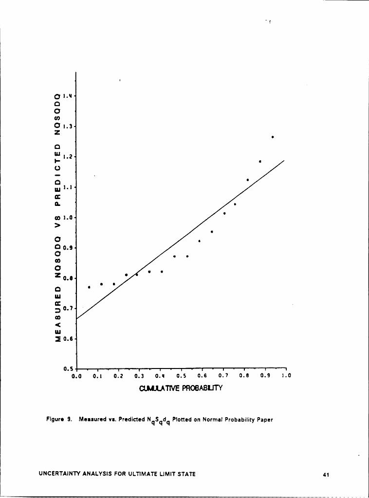
Figure 9. Measured versus Predicted NqSqdq Plotted on Normal Probability Pa-per ................................................... 41

Figure 10. Chart for Estimating Allowable Soil Pressure for Footings on Sand onthe Basis of Results of Standard Penetration Test. ...............53

Figure 11. Stochastic Process NSpT(z) and Bearing Capacity ...............58

Figure 12. C.O.V. Reduction Factor, Type-A Variance Function ..............60

Figure 13. Reliability Index ß versus Different Dead to Live Load Ratios for Ulti-mate Limit State .........................................77


Figure 15. Reliability Index [3 versus Different Dead to Live Load Ratios for Ulti-mate Limit State .........................................81List of Illustrations viii


Figure 17. Reliability Index [3 versus Different Dead to Live Load Ratios for Ser-viceability Limit State .....................................85

Figure 18. Reliability Index B versus Different Dead to Live Load Ratios for Ser-viceability Limit State .....................................86

Figure 19. Reliability Index ß versus Different Dead to Live Load Ratios for Ser-viceability Limit State .....................................87

Figure 20. Performance Factors for Ultimate Limit State ...................94

Figure 21. Performance Factors for Serviceabiiity Limit State ...............95

IList of Illustrations ix

l

List of Tables

Table 1. Bearing Capacity Factors for the Different Prediction Equations .......7

Table 2. Ultimate Bearing Capacity of Shallow Foundation on Sand as Obtainedby Different Equations ......................................9

Table 3. Comparison of Ratio of Measured to Predicted Ultimate Bearing Ca-pacity on Sand for Different Prediction Method ...................10

Table 4. Comparison of the Ratio of Measured to Predicted Settlement (AfterD’Appolonia et al., 1968) ....................................15

Table 5. Ratio of Measured over Predicted NY .........................33Table 6. Ratio of Measured over Predicted SY .........................35Table 7. Ratio of Measured over Predicted lv ..........................36Table 8. Ratio of Measured over Predicted NqSqdq ......................40Table 9. Summary of Model Errors for Ultimate Bearing Capacity ...........42

Table 10. Results of Direct Shear Test on Dense Sand (After Singh and Lee, 1970) 43

Table 11. Results of Direct Shear Test on Loose Sand (After Singh and Lee, 1970) 44

Table 12. Statistics of Friction Angle of Sand ...........................45

Table 13. Summary of Uncertainties in Prediction of Ultimate Bearing Capacity . 45

Table 14. Ratio of Measured to Predicted Bearing Pressure ................52

Table 15. SPT Equipment Variables (After Orchant et al., 1968) ..............63

Table 16. SPT Procedural/Operator Variables (After Orchant et al., 1966) ......64

Table 17. Summary of Uncertainties in Bearing Pressure in Settlement Analysis 65

List of Tables x

Table 18. Bias and Coefficient of Variation for 50-Year Maximum Live Load (After INowak, 1989) ............................................70

Table 19. Summary of Statistics of Load Component .....................72Table 20. Summary of Reliability Analyses for Ultimate Limit State for Span

Length of 40 Feet .........................................78

Table 21. Summary of Reliability Analyses for Ultimate Limit State for SpanLength of 80 Feet .........................................80

Table 22. Summary of Reliability Analyses for Ultimate Limit State for SpanLength of 120 Feet ........................................82

Table 23. Summary of Reliability Analyses for Ultimate Limit State for SpanLength of 160 Feet ........................................84

Table 24. Summary of Reliability Analyses for Serviceability Limit State .......88Table 25. Relationship of Safety Factor, Target Reliability Index and Performance

Factor for Ultimate Limit State ..................,............96

Table 26. Relationship of Ratio of Actual to Predicted Bearing Pressure, TargetReliability Index and Performance Factor for SLS .................97

Table 27. Experimental and Theoretical Values of NY (After De Beer, 1970) . . . 106Table 28. Experimental and Theoretical Values of SY (After Ingra and Baecher,

1983) .................................................108

Table 29. Experimental and Theoretical Values of IV (After Ingra and Baecher,1983) .................................................110

Table 30. Experimental and Theoretical Values of NqSqdq (After De Beer, 1970) 112

List of Tables xi

S

Chapter 1

1.1 GENERAL

Load factor design (LFD), adopted by AASHTO in the mid-1970, is currently used for

bridge superstructure design. The AASHTD specifications do not have any LFD pro-

visions for foundations, and engineers use Allowable Stress Design (ASD). The use

of two different design methods - LFD for superstructures and ASD for foundations -

has resulted in inconsistences and duplication of effort, since different sets of loads

are required for the two methods, and has hindered the widespread adoption of Load

Factor Design. Another Iimitation of the current AASHTO specifications and other

deterministic design procedures is that uncertainties in load and resistance are not

explicitly considered in the design process, resulting in nonuniform risk levels. Thus,

a study to develop a rational load factor design method for bridge foundations was

irrrnooucrion 1

I

necessary in order to develop a consistent approach to the design of bridge super-

structures and foundations.

1.2 OBJECTIVE AND SCOPE

The main objective of this study is to develop performance factors for shallow bridge

foundations for both ultimate and serviceability limit states. A reliability-based ap-

proach is used to calibrate the performance factors with existing allowable stress

method. This study begins with a review of current design practice and basic

reliability-based design concepts. Next, the mathematical formulation for computing

reliability indices for different limit states is presented. This is followed by a dis-

cussion of the statistical analyses performed to obtain uncertainties in Ioads, soll

properties and design equations. The next step is to compute reliability indices for

existing designs for different load combinations and dead to live load ratlos. The last

task is code calibration and determination of performance factors.

1.3 ORGANIZA TION

ln Chapter 1, the motivation, approach and scope of the study is described. Chapter

2 discusses current design practice for shallow foundations, and limit states and

reliability-based design concepts. Chapter 3 presents the reliability model for deter-

mining ultimate bearing capacity; the uncertainties in modeling and design parame-

lNTRoouc‘rioN 2

ters are also evaluated. Chapter 4 presents the reliability model for serviceabilitylimit state and the evaluation of model uncertalnty, inherent variability, and system-atic error resulting from soil exploration. Statistics of dead and live loads on brldgesare presented in Chapter 5. Chapter 6 presents the results of the reliability analysis,code calibratlon and the determination of performance factors consistent with se-lected target reliability indices. Chapter 7 contains a summary of the work, a dis-cussion of the results of reliability analysis, and suggestions for future study.

lN‘rRooucTloN 3

l

Chapter 2

2.1 GENERAL

Many design codes based on the load and resistance factor design (LRFD) format

have been developed in the past few decades. They include the Danish Code of

Practice for Foundation Engineering (1985), the Ontario Highway Bridge Design

(OHBD) code (1983), and AISC Steel Specifications (1986). These design codes have

recognized the existence of uncertainties in design practice and were developed us-

ing reliability theory and the concept of limit states.

In this chapter, a review of current practice for shallow foundation design is pre-

sented. The limit states and the sources of uncertainty in current shallow foundation

design are discussed. Finally, the concept of probability-based design is presented. '

LITERATURE REVIEW 4

l2.2 CURRENT PRACTICE FOR SHALLOW FOUNDATIONDESIGN

Allowable stress design, also called working stress design, is the usual method used

for the design of bridge foundations. ln the allowable stress design method, the

safety of a structure ls determined by restricting the stress due to applied loads

(calculated from an elastic analysis) to a value less than or equal to the allowablestress. The allowable stress is usually determined by dividing the yield or ultimate

strength of the material by a suitable safety factor. The statistical nature of the Ioads,

and the fact that different types of loads (for example, dead load and live load) havedifferent levels of uncertainty are not incorporated in the design philosophy. Design

loads are determined and their effects on the structure are then analyzed in a

deterministic way.

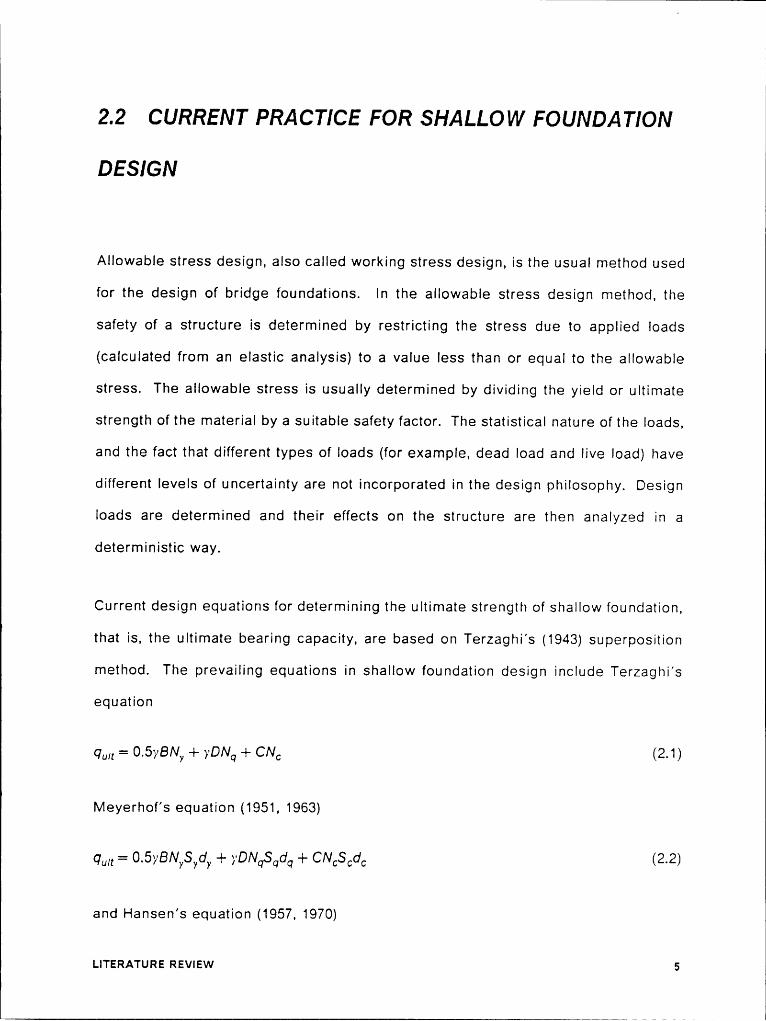
Current design equations for determining the ultimate strength of shallow foundation,

that is, the ultimate bearing capacity, are based on Terzaghi’s (1943) superposition

method. The prevalling equations in shallow foundation design include Terzaghi’s

equaüon

qu,) = 0.5yBNy -1- yDNu + CNC (2.1)

l\/leyerhof’s equation (1951, 1963)

qu,) = 0.5yBNySydy -1- ;·DNuSudu + CNuSudu (2.2)

and l—1ansen’s equation (1957, 1970)

UTERATURE Rsvusw 5

qu,) = 0.5yBNySydy/Y + yDNqSqdq/Q + CNC$CdC/C (2.3)

ln the above equations, q„,, = ultimate bearing capacity of foundatlon, y = unit weightof soll, B = footing width, D = footing depth, Ny, NC, NC = bearing capacity factors,

which are functions of frictional angle, C = cohesion, S,. SC, SC = shape factors,d,, dC, dC = depth factors, and l,, IC, IC = inclination factors. The expressions for thebearing capacity factors are different in each of the above equations and are shown

in Table 1.

The equations for predlcting the ultimate bearing capacity are partly theoretlcal andpartly empirical, so that there ls modeling uncertainty in these equations. There is

also uncertainty resulting from the basic variability in soll parameters such as friction

angle and cohesion. The difference between the predicted and the measured ulti-

mate bearing capacity resulting from the uncertaintles mentioned above can not be

ignored. In a study conducted by Abdul-Baki et al. (1970), the difference between

actual and predicted ultimate bearing capacity of shallow foundations on sand was

investlgated. Ten footings were used to compare the measured ultimate bearing ca-

pacity with results obtained by different prediction methods. The footings varied in

width from 1-ft to 6-ft and had depth to width ratlos in the range of 0.5 to 0.8. The

angle of internal friction, d>,, varied from 25° to 45° and the unit weight of soll varied

from 100 pcf to 130 pcf. The foundatlon dlmensions, soll properties, and results of

predicted as well as measured ultimate bearing capacity are presented in Table 2.

The comparison between the measured and predicted ultimate bearing capacity re-

sults is shown in Table 3. N in Table 3 is the ratio of measured to predicted ultimate

bearing capacity. The coefficlents of varlatlon in Table 3 include the uncertainty as-

sociated with lnherent randomness and random sampllng error.

LITERATURE REVIEW 6

I

T: EC Cb h•U 0>• >•0 U2 2•• mQ cu0 0E EQ Q•• an

vuC,9

TG¤

é°N6 6 Y'

.6 ä—

Ngt = Y EE 9* S ·=€

S K c "Ö •-0 O an c 8E r :1 ~ A°- O G •·: •'Ä, 0 W I ~·* Ig 5 $ • 5- „

I--

Ä E 0 E.9EOU6:u.QU Ag A8 ^ ‘I“6 ‘*'°‘

*.: + I;CQ c 2

2 +I _^ ·€|~ €|<~•+

+ + 2*3* *3* FF F ES E R7

¢OI-U(u.

LITERATURE REVIEW 7

III

*¤3 8Q 3u- Ih• S

•7 cs ~·1 oa (Db C') N N v- 1-fg an r~ r~ •~ <·>¤*UI

ä cÄ GJ•·• W

E ä E E 2 Z, 2- I co cn r~ r~ ané3*° B§ 6aaI: ° ä ¤ v <·¤ rs .-

O U E Q r~ m ao co;,„

éca 0 r~ Ih zu

mc •¤22 •DN QO: •u.q· ,,, ...;‘“

" ä°°E " vav::„g ~c„ . .

ma g B O ngo U Q N QD0); r- v v on‘*¤

NO2:3äägI-Q:

gaE20 .

gcc@2q)4'¤ ~„

s¤ ä ä ä 3 ä E 3 Ei ä 8.-Q -= .„ S 8 8 ** S 2 9 2. 2 2,

: Il II Kl >. Il II II II ll Ilä >~ >• >— vg >„ >— >~ >• >~ >~

9 J «-5 vi 0 ai rd gd ¤¤“ ol IdQ II Il ll Il II II II il ll ll

Q aim aim aim aim aim aim aim aim aim aim'Q S S S S S S S S S S__ 0 v v ¤¤ ew 64 •-· ID •— 04.¤ II Il II II II II Il il I IIg Q Q Q Q Q Q Q Q Q Q

8 cu ca <·> cn v v vII II Il II II ll II II II II6 6 6 6 6 6 6 6 6 6

aaI- r~Illlll lll

- I

LITERATURE REVIEW 8 iIII

—— —- -

-..___ _ _ I

II

äQ

V'

U 'TO

•—O•'¤:E9=¤ä·-

OUJO

PO

E GEbru

r~Q

I'1*

(Dm•J ¢

28°

¤:_§0

•-

:2 °Dc

O

*.99-*62:6-5

.29 °

Q N

2‘¤·- °°.::932

O

Q 7:•——§‘,¤ Nru

Q

wä v~°°’ an

EuO o

PcOm

JQV} O

c•> N

EC Z1-

®

Q} 2OG I-Cc··

V

cc}.

°‘

QR:

CJ

EUQ

v~

ZP

Q

5•4 "TY'

m„_ °’ cä

O c

nnO o

IE S Sr~¤ 2!'*

'_

'-

S: S E T:E Z Ü E c

·¤ ev N Q Qaa 3 '*·

an_ c, Q >~ C

·¤·w 3 ° zuE 1

LITER Tl}^ Rznsvusw 9

From Table 3, it can be seen that Terzaghi’s and Meyerhof’s equations underesti-mate the ultimate bearing capacity while Hansen’s equation overestimates the ulti-mate bearing capacity of shallow foundations on sand. Comparing the statistics ofmeasured to predicted ultimate bearing capacity one may conclude that Hansen’sequation is the best method among the three methods for predicting ultimate bearingcapacity of shallow foundations on sand.

Besides ultimate bearing capacity, bridge designers also need to make sure thatfoundation settlements can be assessed as accurately as possible. It is well knownthat the design of shallow foundations on sand is controlled by settlement criteria inmost cases, except for small footings, say B < 4 feet, at or near the surface. Cur-rently, there are many methods for predicting settlements. These methods are basedon different soil exploration methods. According to Kovacs and Salomone (1982) theStandard Penetration Test (SPT) is the most widely used. They estimated that up to80-90 percent of routine foundation designs in the United States are carried out using

the NSM value. The method has been standardized by ASTM D1586 as "Standard

Method for Penetration Test and Split-Barrel Sampling of Soil" (Bowles, 1982). The

typical setup for the SPT test is shown in Figure 1.

The standard penetration test consists of (Bowles, 1982) using a 140-lb (63.5 kg)

driving hammer falling free from a height of 30 inches (762 mm) to hit an anvil, and

driving the standard split-barrel sampler a distance of 18 inches (460 mm) into the soil

at the bottom of the boring. The NSM value is the number of blows required to drive

the tube the last 12 inches (305 mm). The sampler is pushed a distance of 6 inches

to rest it on undisturbed soil with the blow count recorded. The blow count for each

of the next two 6-in increments ls used as the penetration count unless the last in-

LITERATURE REVIEW 10

„ { {

Figure 1. Typical Instrument Set Up for the Standard Penetration Test: (After Kovacs &Salomone, 1982)


crement can not be completed (either from encountering rock or because theblowcountexceeds 100). In this case the blow count for the last 12 inches iscomputedand

used as the Nsp, value.

Current standard penetration test procedures have some inherent variations betweentests that, according to Ireland et al. (1970), makes this test a "non·standard" stand-ard.

Terzaghi and Peck (1948) were among the first to propose a settlement predictionmethod using the Nsp, value. The chart they developed is shown in Figure 2.

Meyerhof (1965) modified Terzaghi and Peck’s equation and proposed the following

expressions for the settlement of spread footings on sand:

8PaSa = —— for B $ 4 ft (2.4a)Nspr

or

12Pa B 2Sa N$PT<B+1> for B>4t (24b)

in which S_= settlement, in inches; P_= allowable bearing pressure, in tons per

square foot; B = footing width, in foot; NS„= SPT blow count, in blows per foot.

D’Appolonia et al. (1968) conducted a study and found that there were large differ-

ences between the measured settlement and the settlement predicted by the above

two methods. Standard penetration tests were carried out to investigate the settle-

ment of 50 footings. These footings varied in width from 10-ft to 22-ft, with depth to


l

E 65 l/6ry 060:62$2. 5 /V= 50cng cuä -5U 8g 0 4..: ä*7 9 0606*6CJ' G)va ID

SQP

B 93c N·· EE " Z3I0U)9

,3ÄOOSP00 5 /0 /5 20

Width B of Footing in Feet

Flgure 2. Chart for Estimating Allowable Soil Pressure for Footing on Sand on the Basis of Resultsot Standard Penetration Test.: (After Terzaghi & Peck, 1948)

l LITERATURE REVIEW 13l

width ratios in the range of 0.4 to 1.0. The depth of the ground water level below the

base of the footlng varied from the footlng base to 1.0 B. The loads applied to the

footings ranged from 1.5 tsf to 2.5 tsf. The comparison of measured to predicted

settlement from this study is shown in Table 4.

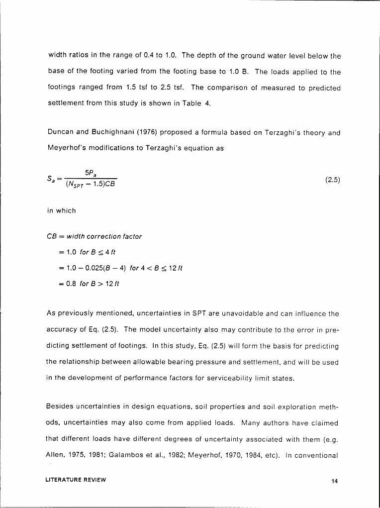
Duncan and Buohighnani (1976) proposed a formula based on Terzaghi’s theory and

Meyerhof’s modifications to Terzaghl’s equation as

s Spa2 6a- (N5,,T—1.5)CB ( ‘ )

in which

CB = width correction factor

= 1.0 forBS4ft

= 1.0 — 0.025(B — 4) for4 < B S 12ft

= 0.8 forB > 12ft

As previously mentioned, uncertainties in SPT are unavoidable and can influence the

accuracy of Eq. (2.5). The model uncertainty also may contribute to the error in pre-

dicting settlement of footings. In this study, Eq. (2.5) will form the basis for predicting

the relationship between allowable bearing pressure and settlement, and will be used

in the development of performance factors for serviceability limit states.

Besides uncertainties in design equations, soil properties and soil exploration meth-

ods, uncertainties may also come from applied loads. Many authors have claimed

that different loads have different degrees of uncertainty associated with them (e.g.

Allen, 1975, 1981; Galambos et al., 1982; Meyerhof, 1970, 1984, etc). ln conventional

UTERATURE Rsvisw 14

Table 4. Comparison of the Ratio of Measured to Predicted Settlement (After D'Appolonia et al.,1968)

Prediction Method

Ratio of Measured Terzaghi and Peck Meyerhofto PredictedSettlement, N

Mean 0.26 0.52

StandardDeviation O.11 0.24

Coefficientof 0.42 0.46Variation

geotechnical design, the Ioads that are applied to the foundation are the unfactored

service or working loads. ln developing a LRFD format for shallow foundation design,

the nature of the uncertainty in different types of Ioads should be included to account

for the different probability of occurrence of these loads. There have been a number

of studies on the statistics of bridge loads. A notable example is the work done by

Grouni and Nowak (1984) which in part forms the basis for the load factors given in

the 1983 edition of Ontario Highway Bridge Design (OHBD) code.

From the above discussion, it is evident that working stress and other deterministic

procedures have a number of limitations. Some of the disadvantages of deterministic

design procedures as pointed out by MacGregor (1979) are as follows:

, LITERATURE REVIEW 15

l

1. Failure to justify the variabllity of Ioads and resistance,

2. Failure to consider the variations in loadings that increase at different rates, and3. Failure to take into account the type of failure or the consequences of failure.

Load and Resistance Factor Design (LRFD) was introduced to overcome some of thelimitations of working stress design methods. LRFD is based on the concept of limitstates, with factors of safety being obtained from a reliability analysis. The LRFD

Fformat is expressed as

¢>R 2 27,0, (2.6)1:1

where d> is the resistance factor, R is the nominal resistance, Q, is the load effect due

to the ith load component, y, is the corresponding load factor, and n is the numberof load components involved in the limit state under consideration. The resistanceand load factors are determined from a reliability analysis. The resistance factor tp,

which is usually less than unity, together with R reflects the uncertainties associatedwith R. The y factors, which are usually greater than unity, reflect the effect of po-tential overloads and uncertainties inherent in the calculation of load effects. Many

countries such as Canada, Denmark and the United States have employed LRFD insome of their design codes. Other countries such as Austria and Japan are devel-oping LRFD codes. Some of the advantages of LRFD (Ellingwood et al., 1980) include:

1. More consistent reliability is achieved for different design cases because thedifferent variabilities of the various design variables are evaluated explicitly and

independently.

2. The consequences of failure can be reflected from selected reliability.

L1TERA‘ruRE Rsvisw 16

I3. The designer can gain a better Insight of the fundamental structural requirements

and of the behavior of the structure in meeting those requirements.4. It ls a tool for incorporating judgment in non-routine situations.

5. lt provides a basis for updating standards in a rational manner.

2.3 LIMIT STATES AND UNCERTAINTIES IN SHALLOWFOUNDATION DESIGN

All structures have in common two basic functional requirements, namely, safety andserviceability. Limit states define the various types of collapse and unserviceabiiity

that are to be avoided (Allen, 1975). According to Meyerhof (1984), collapse or failureof the structure and failure of the soll are ultimate limit states (ULS). Examples ofultimate limit states include lnstabllity by sliding, overturning, bearing capacity fail-ure, uplift, seepage and piping. The occurrence of excessive deformation and dete-rioration are called serviceability limit states (SLS) and include excessive total or

differential settlement, cracking, excessive vibration and corrosion. Although limit

state concepts have only recently been introduced, many researchers have claimed

that they are not new (Simpson et al., 1981; Ellingwood, 1982). For example, in con-ventional foundation design, the ultimate limit state ls considered in the estimation

of bearing capacity, and the serviceability limit state is included in settlement analy-

sis. The occurrence of a limit state Is an event that has a probability of failure asso-

ciated with it. This probability of failure can be evaluated by a systematic analysis

of the uncertainties inherent in design models, equations, and soll parameters.


As we know, the actual outcomes in geotechnical engineering problems are to somedegree unpredictable due to the random nature of soll. Foundation performance isusually dominated by the spatial average value of soll property over an appropriatedomain. According to Tang (1984) there are three types of uncertainties associatedwith the spatial average soll properties. These are:

1. inherent variability- This is the actual variability of soll property in a given domain

although the variability is reduced somewhat from the point variability through

the averaging effect.

2. Statistical uncertainty- This is due to:(i) inherent variability, and (li) random sam-pling and measurement errors in tests on a limited number of soll samples. The

statistical uncertainty can be reduced through increasing the number of test

samples. ·3. Systematic uncertainty- This is the uncertainty resulting from the lncapablllty of

a test to reproduce the in situ property due to factors such as sample disturb— ·

ance, size of specimen, and different stress conditions, etc. This error may not

be diminished as the number of test samples increases because the same kind

of test condition is Iikely to continue to yield consistently high or low property

values. This also applies to the estimation of soll properties using an empirical

callbration formula.

In estimating the ultimate bearing capacity of shallow foundations on sand, uncer-

tainties may be due to the model error, footing shape effect, footing depth effect, load

inclination effect and soll friction angle zb,. The sources of uncertainty that may result

in differences between actual and predicted ultimate bearing capacity are listed in

Figure 3.


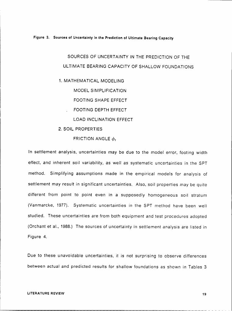
Figure 3. Sources of Uncertainty in the Prediction ol Ultimate Bearing Capacity

SOURCES OF UNCERTAINTY IN THE PREDICTION OF THEULTIMATE BEARING CAPACITY OF SHALLOW FOUNDATIONS

1. MATHEMATICAL MODELING

MODEL SIMPLIFICATION

FOOTING SHAPE EFFECT_ FOOTING DEPTH EFFECTI LOAD INCLINATION EFFECT

2. SOIL PROPERTIES

FRICTION ANGLE tb,

ln settlement analysis, uncertainties may be due to the model error, footing width

effect, and inherent soil variability, as well as systematic uncertainties in the SPT

method. Simplifying assumptions made in the empirical models for analysis of

settlement may result in signlficant uncertainties. Also, soll properties may be quite

different from point to point even in a supposedly homogeneous soil stratum

(Vanmarcke, 1977). Systematic uncertainties in the SPT method have been well

studied. These uncertainties are from both equipment and test procedures adopted

(Orchant et al., 1988.) The sources of uncertainty in settlement analysis are listed in

Figure 4.

Due to these unavoldable uncertainties, it is not surprising to observe differences

between actual and predicted results for shallow foundations as shown In Tables 3

LITERATURE REVIEW 19I

I

Figure 4. Sources of Uncertainty in Settlement Analysis

SOURCES OF UNCERTAINTY IN SETTLEMENT

ANALYSIS OF SHALLOW FOUNDATIONS

1. MATHEMATICAL MODELING

MODEL SIMPLIFICATION

FOOTING WIDTH EFFECT

2. SOIL

INHERENT VARIABILITY

SYSTEMATIC UNCERTAINTY, SPT

and 4. Probabilistic methods are a convenient and useful tool for dealing with un-

certainties in foundation design.

2.4 RELIABILITY-BASED DESIGN

lt has been recognized by many authors that probability theory is a valuable tool for

dealing with uncertainties in engineering problems and many probability~based de-sign formats have been developed (e.g. Cornell, 1969; Ellingwood et al., 1980;

Ravindra et al., 1978; Tang et al., 1976, etc.) In a probabilistic approach, the design

parameters are treated as random variables rather than deterministic constants. The

safety of a structure may be assured in terms of the probability of failure which is

defined as the probability that the system fails to perform its designed function. The


probability of failure can be computed from the distributions of the load and resist-

ance.

The probability of failure is determined from a systematic analysis of uncertainties in

all the design parameters. lt differs from the deterministic safety factor whose deri-

vation depends mainly upon experience and judgment. Although the probabilistic

approach ls more complicated than the deterministic approach, it is more economical

and provides consistent risk levels between different structures and different materi-

als.

A typical reliabilty-based design procedure may consist of the following steps:

1. Develop mathematical expressions for the limit states of interest.

2. Perform uncertainty analyses for all design variables.

3. Compute the reliability index ß for the limit states.

4. Define the load and resistance factors for the selected target reliability index [Y,.

Typically, the limit state equation for a given problem is expressed as

G(x) = R — Q (2.7a)

in normal format, or as

G(x) = /nR — /nO (2.7b)

in lognormal format; in which R is the resistance and Q is the load effect. ln the case

of foundation design, R is the ultimate bearing load for the ultimate limit state. For

the serviceability limit state, R ls the bearing load for specified tolerable settlement.


Several methods have been proposed for computing the reliability index ß. The meanvalue first—order second-moment (l\/IVFOSM) methods were widely employed duringearly versions of reliability·based design codes for structurai design, for example,

LRFD for steel (Ravindra and Galambos, 1978). In the MVFOSM, the reliability indexis based on the mean and standard deviation (the first and second moment) of the

design variables. For the normal format

R' — Öß 6 *—*—6: <2·8>6,, —l- 6Q

For the Iognormal format

E'“ 6

in which Ä'-, 6,,, V,, and 6o, Vo are the mean, standard deviation and coefficient of

variation (cov) of resistance and load, respectively. The coefficient of variation is the

ratio of the standard deviation to the mean. lvl\/FOSM methods have two basic

shortcomings (Hasofer and Lind, 1974) :

1. The limit state function G( ) is linearized at the mean values of the design vari-

ables instead of at a point on the failure surface. This can result in considerable

errors when G( ) is nonlinear because the higher order terms are neglected dur-

ing the Iinearization.

2. Given the same problem, the MVFOSM methods are not invariant for mechan-

ically equivalent formulations.

meRA·ruRe REVIEW 22

Advanced FOSM methods have been developed to overcome the limitations of ÄMVFOSM methods. The basic concepts and analysis procedure for the advanced Ä

FOSM methods have been presented in Ditlevsen (1974), Ellingwood et al. (1980),Hasofer and Lind (1974), and Rackwitz and Fiessler (1978). For a general case wherethe limit state function is a function of several variables, the limit state function canbe expressed as

G(X)=G(X,,X2,X3,...,X„)=0 (2.10)

where X= (X,, X2, X2, , X,,) is the vector of basic state or design variables of thesystem. The function G(X) determines the performance of the system. Geometrically,the limit state function is a n·dimensional surface called the “failure surface". Oneside of the failure surface is the safe state which corresponds to G(X) > 0 , and the

other side is the failure state, which corresponds to G(X) < 0.

The reliability analysis starts with the transformation of the X, variables to a space ofreduced variables using

(X-- Y(2.11)

where x, are reduced variables with zero mean and unit variance. The limit state

function in reduced variables is

G,(x,, x2, x3, , x„) = 0 (2.12)

Failure occurs when G,() = 0. A two-variable problem is shown in Figure 5. The re-Iiability index is defined as the shortest distance between the origin and the failure

surface. The point (x], x2, xg, on G,() = 0 corresponding to this shortest distance


is called the design or checking point. The design point must be determined by si-multaneously solvlng the following equations

öx,oz, (2.13)OG1 2 Q-[ ( öxi l ]

x,1= - aß (2.14)

G2(x;, x2, x2, , x2,) = 0 (2.15)

and searching for the direction cosines a,, that minimize ß. The partial derivatives

are evaluated at the design point.

Since many design random variables do not have a normal probability distribution,

methods for including information on probability distributions have been developed

(Rackwitz and Fiessler, 1978). The basic idea is to transform all non-normal variables

into equivalent normal variables before solvlng the system of equations (2.13) - (2.15).

The algorithm for computing the reliability index using the advanced FOSM methods

can be summarized as follows (Ellingwood et al., 1980) :

1. Define the appropriate limit state; G(X„, X2, X2, , X,) = 0 where the X,’s are the

design variables.

2. Make an initial guess of the safety index ß.

3. Let the initial checking point (X], X2, X2, , Xj„) be equal to the point at the mean

values (X2, X2,

X2,UTERATUREREv1Ew 24

° I

Q > O ·°survivoI °°

X2 —- __• (X. , X2)

Q < O · °fo°I e°• ur 9 so

x' X.

( o)

*2

(1:,:;) } 9( :0. Lfoilure °

(bl

Figure 5. Salety Analysis of Two·variable Problem Using Advanced Method in (a) Original Coor-dlnates and (b) Reduced Coordinates.


il

4. Calculate the mean and standard deviation (XP and of', respectively) of the equiv-alent normal distribution for all non—normal variables.

5. Compute the partial derivatives evaluated at the checking point X}.6. Compute the direction cosines, oz}, using Eq. (2.13).

7. Determine new checking point values from : X} = XP — ot,/36}* and repeat steps 4 to7 until the estimates of the direction cosines oz} stabilize.

8. Calculate the value of ß necessary for G(x}, x}, x}, , x,}) = O , and repeat steps 4I

to 8 until the values of ß on successive iterations differ by some small tolerance.

A computer program was developed to compute the reliability index using the aboveprocedure.

In order to maintain continuity, it was decided to use the same load factors as thoseused in the current AASHTO load factor design specifications. The performance fac-tors are determined by using the reliability indices inherent in current working stress

design methods for shallow foundations and the same load factors as in the current

AASHTO specifications.

LITERATURE Rsvisw 26

ll

Chapter 3

3.1 GENERAL

Deterministic methods have tradltlonally been adopted to predict the ultimate bearlng

capacity of shallow foundations. The accuracy of the results predicted by these

methods depends on a number of factors such as the model used, the choice of soll

parameters and the type of shear failure assumed, etc. As indicated in Chapter 2

there are a number of sources of uncertalnty. In this chapter, the uncertalntles as-

sociated with the prediction of the ultimate bearing capacity are lnvestigated.

uncsntmuw ANALYSIS Fon ULTIMATE LIMIT stAts 27

I

3.2 MODEL FOR ULTIMATE BEARING CAPACITY

PREDICTION

This study is limited to shallow foundations on sand since most bridge shallow foun-

dations are on sand. When other types of soil such as clay is encountered, deep

foundations or pile foundations are used instead of shallow foundations. From the

comparison presented in Chapter 2, it can be observed that Hansen’s equation ex-

hibits less scatter than Terzaghi’s and lVleyerhof’s equation in predicting ultimate

bearing capacity of shallow foundations on sand. Using Hansen's equation as the

basis for the analysis, the ultimate bearing capacity for a shallow footing on sand canbe expressed as:

R = {[0.5yBS,d,/,N,(d>,)] -I- [yDSqdq/qNq(d>,)]}A (3.1)

In Eq. 3.1, N, and N, are bearing capacity factors and are functions of the angle of

internal friction ¢>, ; S, and S, are shape factors; d, and dq are depth factors; I, and I,are load inclination factors; B and D are the width and depth of the footing and A is

the footing area, L is the footing length and i = inclination angle of load. These fac-

tors are defined as '

N, = exp ( -— 2.445 —+- 0.172612) (3.2a)

Nq = exp ( — 1.078 + 0.133«f>) (3.2b)

BS, = 1 —· 0.4 >< T (3.2c)

uNcERTAINTY ANALYSIS FOR ULTIMATE LIMIT STATE 28

I

. BSq=1+sln¢>,x-T (3.26/)

/1 =/C1 = (1 — 0.5 tan i)5 (3.2e)

dq=1+2tand>,x(1-sind>,)2x(-g-) %$1 (3.2f)

d1 = 1 (3.29)

Introducing model correction factors N1 and N, for bearing capacity due to weight and

surcharge gives

R = {N1 x [0.5yBS1d1l1N1(¢>1)] —l— N2 x [yDS,1dq/qNq(<b,)]}A (3.3)

The model correction factors N1 and N, can further be expressed as products of

component correction factors N1 ’s accounting for modellng errors in N1, S1, I1 and

N,’s accounting for modellng errors in N1, S11, dq and I1, respectively. Thus,

fT7

N1 = HN1 (3.4a))=1

H

N2 = ÜN, (3.4b)k=1

where H denotes the product of N1’s and N, ’s. Each of these factors has a mean

value equal to N1 or N, and a coefficient of variation $2,11 or Sl,111. Thus, the expression

for the bearing capacity can be written as I

UNCERTAINTY ANALYSIS FOR ULTIMATE LIMIT STATE 29I

_ _I

/77 /7

R = {[I—[N,][3-5vB$,d,/,^7,($«)] + (3-5)j=1 k=1

The uncertainty in the estimation of the soil parameter qö, can also have a consider-

able influence on the accuracy of the predicted ultimate bearing capacity. The unit

weight of soll, y, has a small coefficient of variation and therefore can be treated as

a deterministic variable.

The mean value of the ultimate bearing capacity R can be expressed as

/T7 /7

R = (EI [I (3-5)}=1 ß<=1

and the variance of R is given by

/77

U; = {[Z(s2§’„J X iT2)][0.6;~es}_6>„iy~y(«)>,)]2}A2}=1

/7

+ (EZIQÄ >< (3-7))«=1

m— ÜN) n — 0N¤ 2 2-l— NJ][O.5yB-Sydy/Y é] + [HNk][;'DSqdq/Q *1+ ]} (Gd, >< A)

1 üb! k=1 üb! 'j=

in which E, and 61,, are the mean and standard deviation of the friction angle tb,.

UNCERTAINTY ANALYSIS PGR ULTIMATE LIMIT STATE 30

I

I

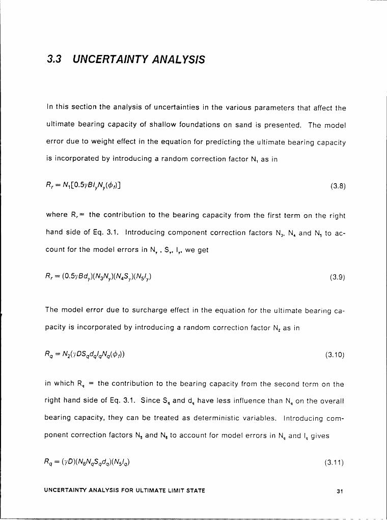
3.3 UNCERTAINTY ANALYSIS

ln this section the analysis of uncertainties in the various parameters that affect the

ultimate bearing capacity of shallow foundations on sand is presented. The model

error due to weight effect in the equation for predicting the ultimate bearing capacity

is incorporated by introducing a random correction factor N, as in

R„ = ^/IIQO-5vB/,N,(d>I)] (3-8)

where R,= the contribution to the bearing capacity from the first term on the right

hand side of Eq. 3.1. Introducing component correction factors N,, N, and N, to ac-

count for the model errors in N, , S,, I,, we get

R. = (9-5>‘8d,)(^/;IN,)(/V4$,.)(/V5/,) (8-9)

The model error due to surcharge effect in the equation for the ultimate bearing ca-

pacity is incorporated by introducing a random correction factor N, as in

R, = N2(yDS,,d,/,N,(qb,)) (3.10)

in which R, = the contribution to the bearing capacity from the second term on the

right hand side of Eq. 3.1. Since S, and d, have less influence than N, on the overallbearing capacity, they can be treated as deterministic variables. Introducing com-

ponent correction factors N, and N, to account for model errors in N, and I, gives

R, = (yD)(N6N,.S,d,)(N,/q) (3.11)

UNcERTAINTY ANALYsIs Fon ULTIMATE LIMIT STATE 31

I

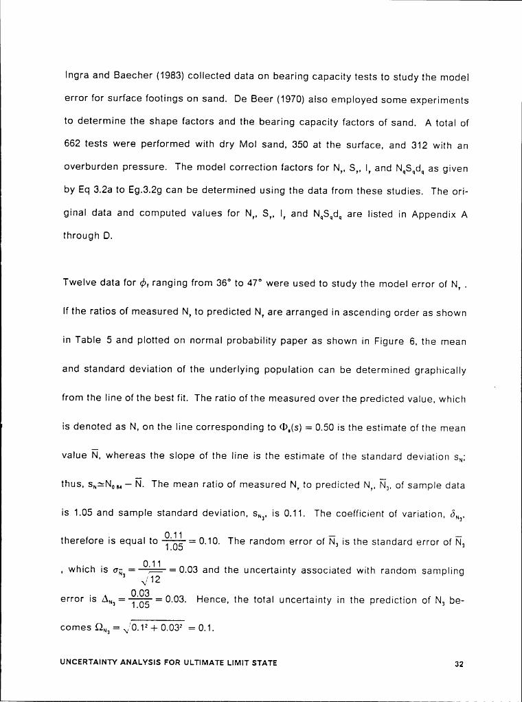
lngra and Baecher (1983) collected data on bearing capacity tests to study the model

error for surface footings on sand. De Beer (1970) also employed some experiments

to determine the shape factors and the bearing capacity factors of sand. A total of

662 tests were performed with dry Mol sand, 350 at the surface, and 312 with an

overburden pressure. The model correction factors for N,, 8,, l, and N,S,,d_, as givenby Eq 3.2ato Eg.3.2g can be determined using the data from these studies. The ori-

ginal data and computed values for N,, 5,, I, and N,S,d, are listed in Appendix Athrough D.

Twelve data for ¢>, ranging from 36° to 47° were used to study the model error of N, .

lf the ratlos of measured N, to predicted N, are arranged in ascending order as shown

in Table 5 and plotted on normal probability paper as shown in Figure 6, the mean

and standard deviation of the underlying population can be determined graphically

from the line ofthe best fit. The ratio ofthe measured over the predicted value, which

is denoted as N, on the line corresponding to <I>,(s) = 0.50 is the estimate of the mean

value N, whereas the slope of the line is the estimate of the standard deviation s„;

thus, s„:N,,, — N. The mean ratio of measured N, to predicted N,, N,, of sample data

is 1.05 and sample standard deviation, s„,, is 0.11. The coefficient of variation, 6,,,,

therefore is equal to %,%-= 0.10. The random error of N, is the standard error of N,

, which is a;3=-ä=0.03 and the uncertainty associated with random sampling

. 0.03 . . . .error is A„,=—F)€= 0.03. Hence, the total uncertainty in the prediction of N, be-

comes QN, = \/0.12 + 0.032 = 0.1.

UNCERTAINTY ANAi.Ysis FOR ULTIMATE Liivur STATE 32

I

Table 5. Ratio of Measured over Predicted NV

m(Ny)m m

(N,),, N —I— 1

1 0.96 0.0772 0.96 0.1543 0.97 0.2314 0.99 0.3085 0.99 0.3856 1.0 0.4627 g 1.03 0.5388 1.05 0.6159 1.10 0.69210 1.16 0.76911 1.18 0.84612 1.28 0.923

Thirty-elght values with % ratlos ranglng from 0.12 to 1 were used to study the model

error of S,. If the ratlos of measured S, over predicted S, are arranged ln ascending

order as shown ln Table 6 and plotted on normal probablllty paper as shown in Flg-

ure 7, the sample mean, N., is 1.2 and the sample standard deviation, s„‘, is 0.2. The

coefflcient of varlation, 6,,,, is equal to -%§-: 0.167 . The random error of Ä, crm, is

$.2.:: 0.03, and the uncertainty associated with the random sampllng error ls* 38xi

AN, :%*%-3- = 0.025. The total uncertalnty in the prediction of N, becomes

QN, = V//0.167* —I— 0.03* = 0.17 .

Thirty-three data for tan i ranglng from 0.11 to 0.58 were used to study the model error

of I,. If the ratlos of measured I, over predicted I, are arranged in ascending order I

IIUNCERTAINTY ANALYSIS FOR ULTIMATE LIMIT STATE 33I

1

I.:

ilq

0

¤¤ 1.1Z •

¤ .

1.2O •

QC

¢ ••

G I.0 • •> . . ·IZ 0.1OIIJ o.•ü(

.

I 0.7

0.6

0.50.0 0.1 0.2 0.3 0.lI 0.S 0.6 0.7 0.8 0.9 I.0

CLMLATIVE PROBABUTY

Figure 6. Meesured over Predicted NY Plotted on normal Probability Paper

UNCERTAINTY ANALYSIS FOR ULTIMATE LIMIT STATE 34

I

Table 6. Ratio of Measured over Predicted Sv

(Sy)m mm (6,),, N + 11 0.94 0.0262 0.97 0.0513 1.0 0.0774 1.03 0.1035 1.03 . 0.1286 1.04 0.1547 1.05 0.1798 1.05 0.2059 1.05 0.23110 ‘ 1.07 0.25611 1.08 0.28212 1.09 0.30813 1.09 0.33314 1.10 0.35915 1.11 0.38516 1.11 0.41017 1.12 0.43618 1.15 0.46219 1.17 0.48720 1.17 0.51321 1.18 0.53822 1.20 0.56423 1.20 0.59024 1.20 0.61525 1.22 0.64126 1.23 0.66727 1.23 0.69228 1.25 0.71829 1.33 0.74430 1.34 0.76931 1.37 0.79532 1.38 0.82133 1.38 0.84634 1.40 0.87235 1.42 0.89736 1.50 0.92337 1.67 0.94938 1.70 0.974


I

1.1 ••

G

QLUI-Q I.5 'Olu •G llq

·• •

•

> ÜI.3

GG •

Q ·• •

ILI I.2 • • •• • •

: •G< . . ‘

•• ••• •

I.0 ••

•

0.9E

0.0 0.1 0.2 0.3 0.¤ 0.5 0.6 0.7 0.8 0.9 l.0

CLM..LATTVE PROBABLITY

Figure 7. Measured over predlcted SY Plotted on Normal Probability Paper


l

as shown in Table 7 and plotted on the normal probability paper as in Figure 8, the

sample mean, N,, is 0.95 and the sample standard deviation, $,,5, is 0.19. The coeffi-. . . . 0.19 — .clent of varlatlon, 6,,5, IS equal to ü§=0.2 . The random error of N,, 6%, IS

0.19 O . . . . ..03 and the uncertalnty assoclated wlth random sampllng IS

A,,5 0.03 The total uncertalnty in the prediction of N, is then

· $2,,5 = ,/0.22 + 0.03* = 0.2 .

. B . . 1 . „ OData wlth T ratlos ranglng from 1 to F, and qö, ranglng from 33 to 41 were used to

study the model error of N,S,dq . lf the ratlos of measured N,S,d, over predlcted

N,S,d, are arranged in ascending order as shown ln Table 8 and plotted on normal

probability paper as in Figure 9, the sample mean, N-, ls 0.93 and the sample stand-

ard deviation, $,,5 , is 0.15. The coefflcient of varlation ls equal to %: 0.16. Therandom error of N,, ugs , ls @:0.0375 and the uncertalnty associated with the116\/

. . 0.0375 . . . .random sampllng IS A,,5 =—CE-{-= 0.04 . The total uncertalnty ln the predlctlon of

N, ls $2,,5 = ,/0.16* + 0.04* = 0.16.

The mean values and coefficients of varlation for the correctlon factors are summa-

rized in Table 9.

uNcERTAlNTv ANALYSIS Fon ULTIMATE l.llvllT STATE 37

1

Table 7. Ratio of Measured over Predicted lv

(Iv)¤'• TT]m (1,), N + 1

1 0.60 0.032 0.60 0.063 0.61 0.094 0.66 0.125 0.67 0.156 0.67 0.187 0.76 0.218 0.81 0.249 0.82 0.2610 0.85 0.2911 0.86 0.3212 0.88 0.3513 0.89 0.3814 0.89 0.4115 0.89 0.4416 0.90 0.4717 0.90 0.518 0.92 0.5319 0.94 0.5620 0.95 0.5921 1.0 0.6222 1.04 0.6523 1.1 0.6824 1.11 0.7125 1.13 0.7426 1.15 0.7627 1.15 0.7928 1.16 0.8229 1.17 0.8530 1.19 0.8831 1.19 0.9132 1.21 0.9433 1.27 0.97

UNcERTA1NTY ANALYSIS FOR ULTIMATE LIMIT STATE 38

’ S

I.S

I.!

I! 1.3•

QILIP I.2

·*

0; U O

Q O

I0-

|I° •

>•

O•" 0.9 • ,

·• •

O • •IHg o.a ° °

•<gg .0.7 •

• •

0.6 • • °

0.50.0 0.l 0.2 0.3 0.1 0.5 0.6 0.7 0.8 0.9 I.0

QJALATIVE PROBABIJTY

Figure 8. Measured over Predlcted lv Plotted on Normal Probability Paper


l

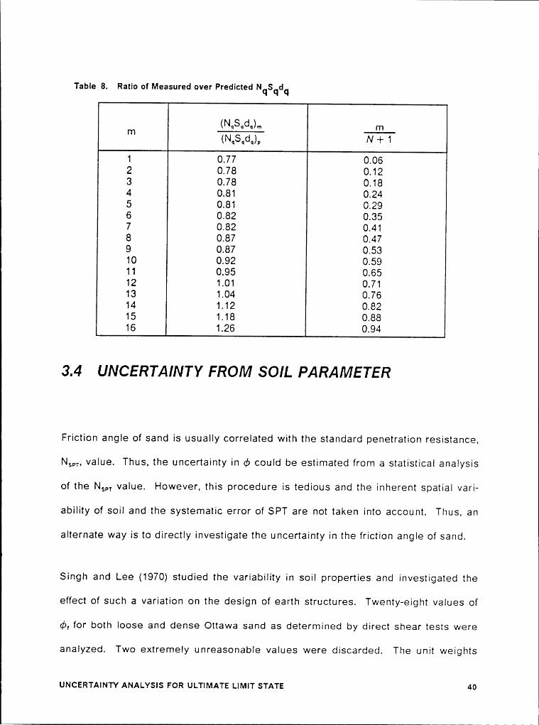
Table 8. Ratio of Measured over Predicted NqSqdq

m (N¤S¤d¤)r¤ |'T1(NqSqdq)„ N —l— 1

1 0.77 0.062 0.78 0.123 0.78 0.184 0.81 0.245 0.81 0.296 0.82 0.357 0.82 0.418 0.87 0.479 0.87 0.5310 0.92 0.5911 0.95 0.6512 1.01 0.7113 1.04 0.7614 1.12 0.8215 1.18 0.8816 1.26 0.94

3.4 UNCERTAINTY FROM SOIL PARAMETER

Friction angle of sand is usually correlated with the standard penetration resistance,

NW, value. Thus, the uncertainty in d> could be estimated from a statistical analysis

of the Nsp, value. However, this procedure is tedious and the inherent spatial vari-

ability of soil and the systematic error of SPT are not taken into account. Thus, an

alternate way is to directly investigate the uncertainty in the friction angle of sand.

Singh and Lee (1970) studied the variability in soil properties and investigated the

effect of such a variation on the design of earth structures. Twenty-eight values of

da, for both loose and dense Ottawa sand as determined by direct shear tests were

analyzed. Two extremely unreasonable values were discarded. The unit weights


5Q 1.lIQOWO 1.3Z

O

O“" 1.2}- •

OE ° ·N 1.I¢1 •

•m 1.0> •G OO 0.sG • •WOZ•

•¤ ÜIII

.

:°•7 ‘

W(III} 0.6

0.50.0 0.I 0.2 0.3 0.1 0.5 0.6 0.7 0.0 0.9 1.0

C1.M.I.A'I"|VE PFIOBABIJTY

Flgura 9. Meaaured va. Pradicted NqSqdq Plotted on Normal Probabillty Paper


I

I

Table 9. Summary of Model Errors for Ultimate Bearing Capacity

Variable Correction Factor Mean C.O.V.

N, N, 1.05 0.1

6, N, 1.2 0.17

N,S,l, N, 1.2 0.28

N,S,d, N, 0.93 0.16

N,S,d,l, N, 0.66 0.26

ranged from 88 pcf to 103 pcf for loose sand and from 93 pcf to 122 pcf for dense sand.

Six triaxial tests were also performed to compare the friction angle obtained from

triaxial tests with the values obtained from direct shear tests. Results from these two

different tests were found out to be in good agreement. The tests on dense sand are

shown in Table 10, while the results for loose sand are shown in Table 11. From theanalysis of the above data, the mean friction angle of loose sand can be estimated to

be 30° with a c.o.v. of 0.17. The mean friction angle of dense sand is 36° with a c.o.v.

of 0.18. The statistics of friction angle of sand are summarized in Table 12. The re-

sults can be assumed to be the spatial statistics of sand.


Because of the plain strain effect, a large value of da, should be used for long footings I

(l\/leyerhof, 1965). The relationship can be expressed as follows:

Bd>BC=dJ!(1.1—0.1—T) (3.12)

where ib, is the value of d> obtained from triaxial tests and ibac is the value of d> used

for computing bearing capacity.Table 10. Results of Direct Shear Test on Dense Sand (After Singh and Lee, 1970)

Interval Number of Fraction of totalObservations Observation

25°~27° 1 0.03827°~29° 1 0.03829°~3I° O O31°~33° 3 0.11633°~35° 4 0.15435°~37° 2 0.07737°~39° 6 0.23139°~41° 6 0.23141°~43° 2 0.07743°~45° O O45°~47° O Ü47°~49° Ü Ü49°~51° 1 0.038

. Total = 26 1.00


I

Table 11. Results of Direct Shear Test on Loose Sand (After Singh and Lee, 1970)

lnterval Number of Fraction of totalObservations Observation

17°~19° 1 0.038l9°~2l° O O2l°~23° O O23°~25° 2 0.07725°~27° 2 0.077· 27°~29° 2 0.07729°~31° 3 0.11531°~33° 10 0.38533°~35° 3 0.11535°~37° 2 0.07737°~39° 0 0.039°~41° 1 0.038

Total =26 1.00

3.5 5UIl/Ill/IARY OF UNCERTAINTIES IN BEARING

CAPACITY PREDICTION

ln the previous sections, uncertainty analyses of the major factors affecting ultimate

bearing capacity for shallow foundations on sand were presented. The statistics of

the model error and friction angle, gb, , for the prediction of the ultimate bearing ca-

pacity are summarized in Table 13. The overall uncertainty of ultimate bearing ca-

pacity of shallow foundations on sand then can be evaluated using equations 3.6 and

3.7.

u~c&RTAi~Tv A~Ai.vsis Fon ULTlMATE Liiviir sTA‘rE 44

I

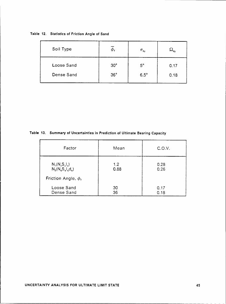
Table 12. Statistics of Frlction Angle of Sand

Loose Sand 30° 5° 0.17Dense Sand 36° 6.5° 0.18

Table 13. Summary of Uncertainties In Prediction of Ultimate Bearing Capacity

Factor Mean C.O.V.

N,(N,s,1,) 1.2 0.28N,(1~1„6„1.„6„) 0.88 0.26Friction Angle, tb,

Loose Sand 30 0.17Dense Sand 36 0.18


l

Chapter 4

UNCERTAINTY ANALYSIS FOR SERVICEABILITY

LIMIT STATE

4.1 GENERAL I

Settlement is an important consideration in the design of bridge foundations. ln fact,

for most shallow foundations, settlement controls the design rather than bearing ca-

pacity. ln this chapter the model for the serviceability limit state is presented. Then

the results of the investigation of model uncertainty, inherent variability and system-

atic error is presented. To evaluate the individual contribution of inherent spatial

variability, N, , and systematic error, N,, to the overall uncertainties, an equivalent

random field model for combined correction factors N,N, is developed and the relative

contribution of N, and N, is studied. The final section presents a summary of the re-

sults of the uncertainty analysis.

UNCERTAINTY ANALYSIS FOR SERVICEABILITY I.IIvIIT STATE 46

LI

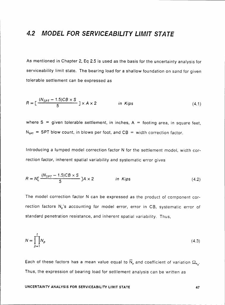
I4.2 MODEL FOR SERVICEABILITY LIMIT STATE

As mentioned in Chapter 2, Eq 2.5 is used as the basis for the uncertainty analysis for

serviceability limit state. The bearing load for a shallow foundation on sand for given

tolerable settlement can be expressed as

(N — 1.5)CB x SR=r—-Ä—?l——]x4><2 in Kips (4.1)

where S = given tolerable settlement, in inches, A = footing area, in square feet,

NS,. = SPT blow count, in blows per foot, and CB = width correction factor.

Introducing a lumped model correction factor N for the settlement model, width cor-

rection factor, inherent spatial variability and systematic error gives

(NSPT —1.5)CB >< S l _R = N[——T——i]A >< 2 In Kips (4.2)

The model correction factor N can be expressed as the product of component cor-

rection factors Np’s accounting for model error, error in CB, systematic error of

standard penetration resistance, and inherent spatial variability. Thus,

ziv = NN), (4.3)

P=I

Each of these factors has a mean value equal to N, and coefficient of variation §2„p.

Thus, the expression of bearing load for settlement analysis can be written as

UNCERTAINTY ANAI.)/sls FOR ssRvIcEAaII.I‘rv LIMIT STATE 47

l

i

I (Nsp, —1.5)CB >< SR = [HNp][ ————§——-l] >< A >< 2 in Kips (4.4)p=^l

To evaluate the variance of R, it is easier to rewrite as

—

R = [l—[Np]R, (4.6)p=1

_ _ (Nsp,—1.5)><CB><S><2 _in which R, The effect of random systematic error and

inherent spatlal variability of soll parameter on bearing load is incorporated in the

evaluation of the statistics of R,. However, it is desirable that each of these effects

be represented by one random variable similar to Np so that the influence of each

factor on the bearing load can be conveniently investigated and measured. There-

fore, the bearing load for given tolerable settlement can be written as

4 —15Ö§xSxAx25

where psp, is the mean value of Nsp,. Observe that RN is simply the bearing load de-

termined by Eq. 4.4 with the penetration resistance, Nsp,, and CB set equal to their

mean values, psp, and and all model correction factors set equal to one. In fact,

RN is the deterministic bearing load. Thus, the bearing load in Eq. 4.4 can be ex-

pressed as

u~cERrAi~Tv ANA1.vsis l=oR sERvicEAaiLiTv LIMIT STATE 48

ZR — [HN Jl Ä iRp=1

z

P=1w=t+2

=tP=‘l

. .\ R1 . . . .in which the product of N,N, =?; and N, and N, represent the indlvidual effect of in-

N

herent spatial variability and systematic error of soil properties on the bearing load.

Thus, the mean value of bearing capacity in Eq. 4.7 can be expressed as

W

Fi = [I |r7,,]R,, (4.8)p=1

and the variance of R is given by

W .gf, = X N; X (écl )2) (4.9)x>=l p

where w = t+2, based on the assumption that all the correction factors are statis-

tically independent random variables.

uucsarmurv ANA1.vsis Fon ssRvic6A6¤Li·rv Limrr sure 49

l

l

4.3 ll/IODEL UNCERTAINTY

ln a probabilistic approach, the model error is assumed to be dominated by the pen-

etration resistance Nsp,. Thus, the model error Nm in the bearing capacity equation

may be evaluated from measured pressure (q„) obtained from test data

qON"' _

(NSPT —1.5)CB x S (410)5

provided that NSM, S and foundation dimensions are available.

For this study, a data base of 200 records of settlement of foundation collected by

Burland and Burbridge (1985) was used to estimate the model error. The data set

included observed settlements of shallow foundations estimated using different types

of testing methods, including SPT, CPT (cone penetration test), oedometer and plate

loading test. Only the data from tests performed using the SPT were analyzed. Data

which gave extremely large or extremely small measured over predicted ratlos of

bearing pressure were excluded from this analysis. A ratio of measured over pre-

dicted bearing pressure greater than 2.5 is considered extremely large while ratio

smaller than 0.5 is considered extremely small. A total of 27 values was included in

this study. The ratio of measured to predicted bearing pressure, Nm, ranged from 0.55

to 2.47 as shown in Table 14. The mean, Kim, of sample data is 1.4 and sample

standard deviation s„m is 0.55. The coefficient of variation ö„m, therefore, is equal to

uNcERTAiNTv ANAt.vsis Fon sERvlcEABlLl1Y LIMIT STATE so

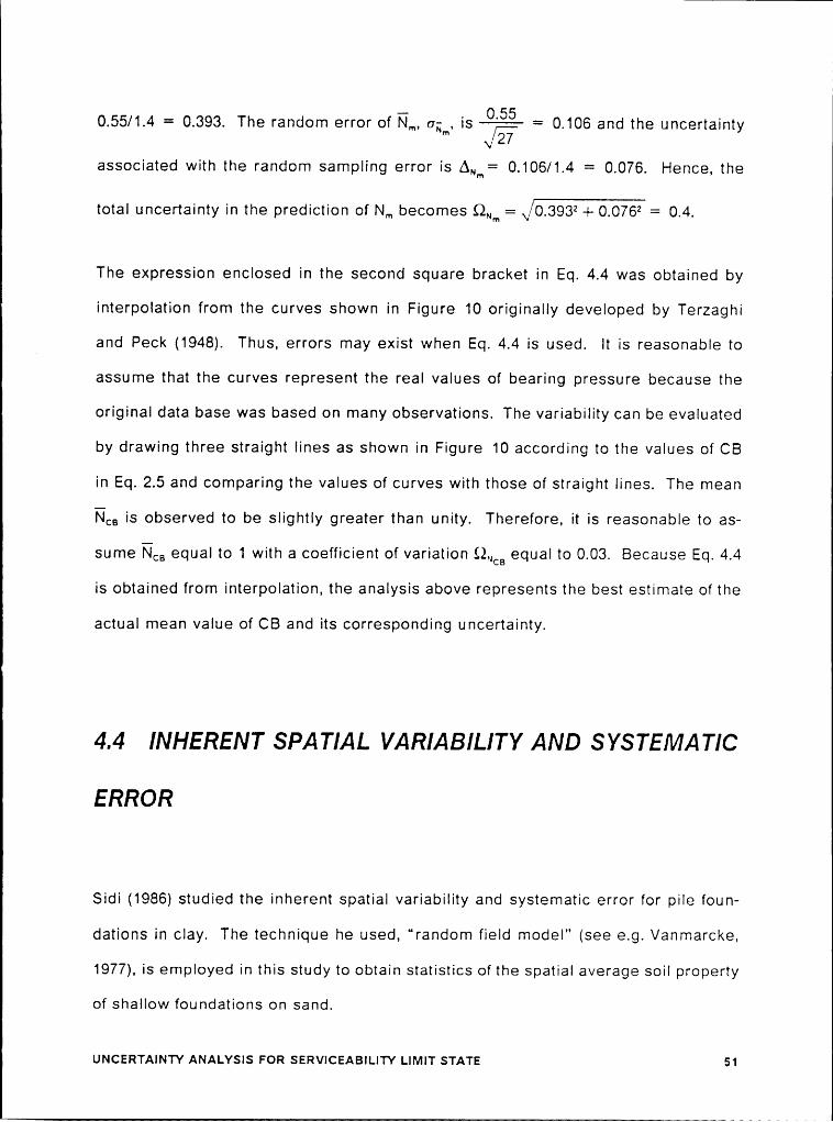
0.55/1.4 = 0.393. The random error of Nm, 6; , ls = 0.106 and the uncertainty"‘27

associated with the random sampling error ls A„m= 0.106/1.4 = 0.076. Hence, the

total uncertainty in the prediction of N„, becomes QNm = ./0.3932 —l- 0.0762 = 0.4.

The expression enclosed in the second square bracket in Eq. 4.4 was obtained by

interpolation from the curves shown in Figure 10 originally developed by Terzaghi

and Peck (1948). Thus, errors may exist when Eq. 4.4 is used. lt ls reasonable to

assume that the curves represent the real values of bearing pressure because the

original data base was based on many observations. The variablllty can be evaluated

by drawing three straight lines as shown in Figure 10 according to the values of CB

in Eq. 2.5 and comparing the values of curves with those of straight lines. The mean

NC., ls observed to be slightly greater than unity. Therefore, it ls reasonable to as-

sume NC., equal to 1 with a coefficlent of variation £2,,CB equal to 0.03. Because Eq. 4.4

is obtained from interpolation, the analysis above represents the best estimate of the

actual mean value of CB and its correspondlng uncertainty.

4.4 INHERENT SPATIAL VARIABILITY AND SYSTEMATIC

ERROR

Sidi (1986) studied the inherent spatial varlabllity and systematlc error for plle foun-

dations in clay. The technique he used, “random field model" (see e.g. \/anmarcke,

1977), ls employed in this study to obtain statistics of the spatial average soll property

of shallow foundatlons on sand.

uNcERTAlNTv ANA1.vsls Fon sERvicEABu.lTv Lnvur STATE 51

Table 14. Ratio ol Measured to Predicted Bearing Pressure

mm Nm m+11 0.55 0.03572 0.63 0.07143 0.68 0.10714 0.72 0.14295 _ 0.77 0.17866 0.78 0.21437 0.88 0.258 0.93 0.28579 0.96 0.321410 1.03 0.357111 1.13 0.392912 1.32 0.428613 1.42 0.464314 1.5 0.515 1.53 0.535716 1.56 0.571417 1.66 0.607118 1.73 0.642919 1.79 0.678620 1.82 0.714321 1.85 0.7522 1.89 0.785723 1.89 0.821424 1.93 0.857125 2.0 0.892926 2.26 .928627 2.47 0.9643

Soil parameters are partly correlated between any two points within the scale of

fluctuation in both horizontal and vertical directions (Vanmarcke, 1977). Besides the

spatial variation, uncertainties in soll properties also include systematic errors.

Therefore, a model that is able to incorporate both inherent spatial variability and

systematic error is needed for a realistic evaluation of these uncertainties. In the

next section, an attempt is made to express these new components of uncertainties

in a form so that their statistics could be easily combined with those obtained earlier

for the other modeling errors.

UNCERTAINTY ANALYSIS FOR SERVICEABILITY LIMIT STATE S2

{ I

E Öaal/arg 06056

E§____3;2

D .Cö’ Tä2 O 4.; 3Ü; i 060:6*In m¤.¤

_;

LI? 2.2 g&’ "’ Z3tn .g /*76*6/zu/27Eguu / ‘

ALoose00 5 /0 /5 20

Width B of Footing in Feet

Figure 10. Chart lor Estlmatlng Allowable Soll Pressure lor Footlng on Sand on the Basls of Re-sults ol Standard Penetration Test.: (Alter Terzaghi and Peck, 1948)

UNCERTAINTY ANALYSIS FOR sERvIcEABILITY LIMIT STATE 53

l

4.4.1 Equivalent Random Variable Model

The effect of inherent spatial variability (N,) and random systematic error (N,) of soll

properties associated with settlement analysis of shallow foundation on sand ls given

bv

R1N,N, = E; (4.11)

where R„ and R, are factors previously defined in section 4.2. From basic theory of

probability, the mean and variance of N,N, are given by

1 ...E[^//Vs] = *,5- {R1) (4-12)iv

and

VAR[N,N,] = -1; {og} (4.13)RN

Vanmarcke (1977) has claimed that there is always a reductlon in the coefficient of

variation of the spatial average as compared to that of the average point. The amount

ol reductlon is dependent on the variance function which is a function of the scale of

fluctuation. The scale of fluctuation, 0, is a measure of the distance within which the

soll property demonstrates a strong correlation from point to point in a soll stratum.

For a shallow foundation on sand, a 3-dlmensional random field model can be used

to express the relationship between inherent spatial variability and point variability

as (Vanmarcke, 1983)

uNcERTA¤Nw AivAi.vsis Fon sERvlcEAaiLiw t.iivuT STATE 541

l

Qspm = V(><)l“(yl><)l“(Z|><- y)92pO„„ (4-14)

in which 9,,,,,,, = spatial c.o.v.; I"(x) = variance function in x—direction; I"(yIx) =

conditional variance in y-direction given the variance function in x-direction;

l”(zIx, y) = conditional variance function in z·direction given the variance functions

in x and y directions; §2„,„, = point c.o.v.

It is difficult to obtain the conditional variance functions in geotechnical problems.

However, to study the problem it is convenient and reasonable to assume that the

variance functions are independent. Also, it can be assumed that soil properties are

the same in horizontal directions; that is, the scale of fluctuation ( 0, and Oy ) are the

same. Therefore, Eq. 4.14 can be rewritten as

2Qspatial = rxryrzgpolnt = rxrzglpolnt (4-15)

ln order to obtain the variance functions in x and z directions, consider a

1-dimensional random field model for the z direction first. lt is known that penetration

resistance varies with depth even though both soil density and components are the

same. Thus, the uncertainties of the penetration resistance with depth may be mod-

eled by a one dimensional random field as shown in Figure 11. According to

the 1-dimensional model proposed by Vanmarcke (1977), the mean value of N,N, can

be expressed as

uNcERTAiNTv ANAi.vsis Fon SERVICEABILITY LIMIT STATE ss

1E[^/,^/6] = WENN1 L —

(TI NSpT(z) dz —-1.5)CB >< A >< S >< 2

RN EL 6 LL N __dz -1.6106 X A X s X 2 (M6)

0· RN EL 6A X s X 2

The variance is

1VARUV/V6]

X s X A X 21 0= ———VAR[RN 5 L

.. @-282AQ ><4 E 2 L L -2-2“ 25 X R2 ( LN/V] O O NNNSPT}N

2 (4.17)

2ÖEQSQAQ X 4 2 L L PM (Z1·Z2)°~ dZ1dZ2= 25 X R2 {(41%,,,+ 1)[

O O><N

CTEQSQAQ XAN

u~csRrA1~rv A~ALvs1s r=¤R SERVICEABILITY LIMIT sure 56

l

in which L = averaging distance; p„$PT = correlation function of /\7S,,,(z) between 2,

and 2,; o„$PT = point standard deviation of /{/$,,,(z) accountlng for random spatial vari-

ability at a point; A„sPT = coefficient of variation of systematic model error of /<l$,„,(z)

and l”§(L) is the variance function of /<J$,,,(z) defined as

L L2 0 0I“A(L) = ————5—-l-—— (4.18)

L

From Eq. 4.16, it can be seen that both the inherent spatial variability and random

systematic error in soil parameter associated with bearing capacity of shallow foun-

dations on sand are included in the model. The influence of inherent spatial vari-

ability can thus be analyzed by using an appropriate variance function. Vanmarcke

(1979) pointed out that the scale of fluctuation can be a signiflcant factor in random

field problems. Mathematically, it can be expressed as

2 OO9 =JL1;1oLVA(L)=f p,.(u)<r/r (4-19)

where p„(;L) = correlation function. lf L goes to infinity, then I"§(L) willapproachFrom

observations of the relationship between the scale of fluctuation 8 and averag-

ing distance L, Vanmarcke (1979) proposed an expression for I“,,(L) as shown in Fig-

ure 12, namely,

l”A(L) = 1 8 2 L (4.20a)

9 1. Ü S L (4.20b)

UNCERTAINTY ANAl.Ysls Fon SERVICEABILITY LIMIT STATE 57

N „„ <Z>•J

SAND ~ éN ,„iS éR E+·„1· > ¤U E-•— Q

EIN SPT (2)] L L _NSpr(Z) dz X A X S X 2R ' ‘;‘U—·——

Flgure 11. Stochastlc Process NSP1-(2) and Bearlng Capacity

UNCERTAINTY ANALYSIS FOR SERVICEABILITY LIMIT STATE 58

This approximation gives satisfactory results in most cases.

4.4.2 Evaluation of N, and NS

From Eq. 4.16 and 4.17, the combined effect of the inherent spatial variability and

random systematic error can be assessed. However, it is desirable to evaluate the

individual contribution of N, and N, to the overall statistics of R. Assuming that there

is no systematic error in determining the Soil parameter, i.e., /7,, = 1 and ANSPT = 0,

Eqs. 4.16 and 4.17 reduce to the mean and variance of N,. Similarly, statistics of N,

may be obtained by assuming that there is no inherent spatial variability of soil

property included, namely by letting the variance function I",,(L) equal to unity.

ln order to evaluate N,. the c.o.v. of Nsp, was assumed to be 0.42 which represents a

reasonable but conservative estimate (Briaud and Tucker, 1984). Then, from previous

derivations, the overall variance function can be expressed as

I"(D) = I“2(x)I"(z) (4.21)

where l”(D) = variance function of the interested 3-D domain. According to

Vanmarcke (1977), the value of the scale of fluctuation 0 of SRT is about 8 feet (2.4

meter). For shallow foundations, it is reasonable to assume that the averaging dis-

tance L is equal to two times the footing width (28). Currently, there is no available

data for the scale of fluctuation of SPT in the horizontal direction. However, data from

other tests such as CPT can be employed to estimate the scale of fluctuation for SPT

in horizontal direction. A value of 20 meters to 35 meters of correlation parameter,

b, of CPT on sand in horizontal direction has been proposed in Tang’s work (1979)

uNcERTAlNTY ANALYSIS FOR SERvlcEABll.lTY LIMIT STATE 59

I, I

I.O

I ··~···-· L S 0L 28·· Double Expon Conel. Funcllon

Fu (L) (\ •-—- Sunple Expose. Correl. Functlon\, '*°“* Trldnqulqr Correl. Funcflofl‘(\

0 = $c¤l• ol Flucfuction‘\'\L ¤ Averaqlnq Distancex\< UL

OS \\.

\\\\\\~

\~•

Oo I 5 IO I5 20

9

Flgura 12. C.O.V. Raductlon Factor, Type·A Varlanca Function: (After Vanmarcke, 1979)


where b is equal to A value of 30 meters for b was used in the study of offshorerr

site exploration in North Sea (Wu et al., 1986). Therefore, it is reasonable but con-

servative to assume that the correlation parameter b is equal to 20 meters for SPT

on sands in the horizontal direction. The value of 6 for SPT in the horizontal direction

then is equal to 20 >< J; >< 3.28 = 116 feet. For a shallow foundation of a bridge, the

width of the foundation seldom exceeds 30 feet. Thus, the averaging distance L is

smaller than 60 feet in most cases. Then, according to Eq. 4.20a, the variance func-

tion in the horizontal direction, l”(x) is equal to 1. For a homogeneous soil media, the

mean of the soil parameter at a point is identical to the mean value of the spatial av-

erage (Vanmarcke, 1979), and so the evaluation of for sands from Eq. 4.16 gives a

value of one (that is Ä = 1). The coefficient of variation of inherent spatial variability

N, can be approximately expressed as

QNI = I”2(x) >< I”(z)QNSpT

=1><(-%)%><O.42

8 L (B in feet) (4.22)= 2 X 0.42

- .1:2..

In addition to inherent spatial variability, the variation in the way standard penetration

tests are performed also contribute to the uncertainty in the prediction of bearing

capacity. There are several factors influencing the SPT and they are called system-

atic errors. Orchant et al.(1988) studied the test variability in SPT by reviewing the

previous work (e.g. Bieganousky et al., 1976, 1977; Schmertmann and Palacious, 1979;

Kovacs and Salomone, 1982, etc.) They classified the sources of uncertainties in SPT

UNCERTAINTY ANALYSls FOR SERVICEABILITY LIMIT STATE 61

into two groups: those due to equipment and those due to test procedures. The

factors that influence the SPT results are listed in Table 15 and 16.

Three sets of SPT data were collected to study systematic errors. The first data set

was collected to study the relationship between relative density of cohesionless soils

and Nsp, values. A total of 32 test results (Bieganousky and lvlarcuson, 1976; 1977)

with different types of sand, overconsolidatlon ratio, dry density, relative density,

vertical stress, and depth were obtained. The second data set was collected to in-

vestigate energy transfer of different types of hammer during the standard pene-

tration test. A total of 109 measurements (Palacios, 1977) with the combination of

safety hammer, donut hammer and A-weight rod, AW-weight rod and N-weight rod

were used. The third data set was collected to study the energy delivered by different

drilling systems. Thirty five series (Kovacs et al., 1981) of tests with different combi-

nations of drlll rig model, number of turns of rope around cathead, hammer fall height,

cathead speed and rotation direction, rope size, rope age and type of hammer were

obtained.

Statistical analyses of these three data sets showed that the coefficient of variation

for equipment variability was 5-75 percent and for procedural variability 5-75 percent.

The low value of c.o.v. represents the use of identical equipment and procedures in

each test. The high value of c.o.v. results from no control on equipment and test

procedures. A 12-15 percent correction factor added was included to take into ac-

count random test error. According to Orchant et al. (1988), the c.o.v. due to sys-

tematic error is on the order of 14 to 45 percent. Thus, it is conservative but

reasonable to assume that the mean correction factor for systematic error is equal to

1.0 with c.o.v. of 0.30.

uNcERTAlNTY ANA!.)/Sis FOR SERVICEABILITY LIMIT STATE 62

i

Table 15. SPT Equipment Variables (After Orchant et al., 1988)

Variable Relative Effect on SPT Results

Non-standard sampler moderate

Deformed or damaged sampler moderate

Rod diameter/weight minor

Rod length minor

Deformed drill rods minor

Type of hammer moderate to significant

Hammer drop systems significant

Hammer weight minor

Size of anvil minor

Type of drill rig minor

4.5 SUIVI/l/IARY OF UNCERTAINTIES FOR SETTLE/l/7ENT

ANALYSIS

ln the previous sections, uncertalnty analyses of major factors affecting bearing ca-

pacity for given settlement of shallow foundations was presented. Statistics of each

of these correction factors were obtained in terms of the mean and coefficient of

variation as shown in Table 17. By using the relevant components of the correction

factors, the total uncertalnty in the allowable bearing load of shallow foundations for

given tolerable settlement can be evaluated using equations 4.8 and 4.9. For exam-

uNcERTAlNTv ANAi.vsls FoR sERvicEAaiLlTv LlMiT STATE 63

l

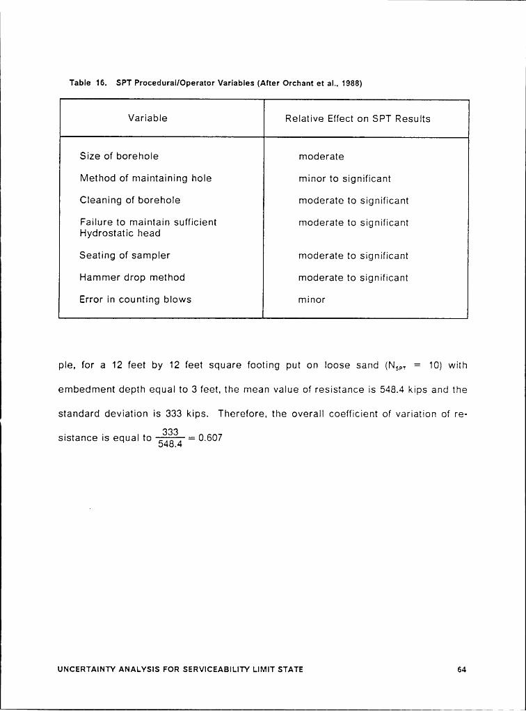
Table 16. SPT ProcedurallOperator Variables (After Orchant et al., 1988)

Variable Relative Effect on SPT Results

Size of borehole moderateMethod of maintaining hole minor to significant

Cleaning of borehole moderate to significant

Failure to maintain sufficient moderate to significantHydrostatic head

Seating of sampler moderate to significant

Hammer drop method moderate to significant

Error in counting blows E minor

ple, for a 12 feet by 12 feet square footing put on loose sand (NW = 10) with

embedment depth equal to 3 feet, the mean value of reslstance is 548.4 kips and the

standard deviation is 333 kips. Therefore, the overall coefficient of variation of re-. . 333sistance us equal to 548.4 — 0.607

uNcERTAlNTv ANAl.YSlS FOR SERVICEABILITY LIMIT STATE 64

ITable 17. Summary ol Uncertainties in Bearing Pressure in Settlement Analysis

CORRECTION FACTOR MEAN C.O.V.

Model Error, N

Duncan & Buchighnani method 1.4 0.4

Width effect,NC,, 1.0 0.03— . . . 1.2Inherent Variabillty, N, 1.0 —:.—

(/ZB

Systematic Error, N, 1.0 0.30(Standard Penetration Test)


l

Chapter 5

GENERAL

Loads on bridges exhibit more variability than loads on other structures. In this study

loads are assumed to be transferred from the superstructure directly to the founda-

tion without any lateral transfer through the abutments. Therefore, the available sta-

tistical data for loads on the superstructure can be directly applied to the foundation.

The different bridge design codes and specifications use different load classifications.

The load classification employed by Grouni and Nowak (1984) for the Ontario Highway

Bridge Design (OHBD) code will be adopted in this study. Grouni and Nowak classi-

fied load components into five categories : (1) dead load, (2) live load and other loads

related to moving trucks, (3) environmental effects, (4) strain—related effects, and (5)

prestressing force. This classification is somewhat different from that in current

s*rATisTics or i.oA¤s 66

l

AASHTO specifications. ln this study, only dead and live Ioads are considered. Also,

not both dead and live loads are normally distributed. However, by central limit the-

orem (Ang and Tang, 1975), their combinations can be considered to be normally

distributed.

5.2 DEAD LOAD

The dead load, D, is from the self weight of the superstructure, sidewalks,

appurtenances, substructure, and other non-structural elements. Dead Ioads may

impose more influence on larger span bridges than short to medium span bridges

due to the higher dead-to-live load ratio of larger span bridges as compared to that

of short to medium span bridges. Variability in dead load results from uncertainties

in the unit weight of different materials. Grouni and Nowak (1984) subdivided the ‘

dead load, D, into three components (i) D,, weight of factory-made members, (ii) D3,

weight of structural components produced in the field and weight of mass concrete,

and (iii) D3, weight of wearing surface. Dead load components are essentially time-

invariant and can be treated as normally distributed random variables.

The distribution parameters, ratlos of the mean to nominal (2.) and coefficients of

variation (V) of dead load were established by an OHBD working committee and

evaluated on the basis of available data. Values of the parameters are 2 = 1.03, 1.05

and 1.05 and V = 0.04, 0.08 and 0.25 for D,, D3, D3, respectively. The highest degreeA

of uncertainty in dead load, D, comes from the weight of wearing surface, D3. How-

ever, D3 is a small portion of the overall dead load and can be assumed to have less

STATISTICS OF LoAos 67

l

influence than D, and DZ on the overall dead load D. Therefore, it is conservative to

assume ,1 = 1.05 and V = 0.10 for the combined dead load effects transferred from

the superstructure to the foundation.

5.3 LIVE LOAD

Live load, L, consists of weight of vehicles on a bridge as well as other loads such

as impact or dynamic effect of a moving truck, I, braking force, centrifugal force, etc.

In the current AASHTO specifications, impact, I, is not considered in foundation de-

sign. Other Iive loads such as braking forces and centrifugal force have almost no

influence on foundations when load effects are transferred from the superstructure to

the foundation. Therefore, only live loads from vehicles need to be considered. Live

load is a time-varying load with a short time span depending on the volume and

composition of traffic using the bridge, which in turn depends on the geographical

location of site and the probability of potential overloads of vehicles. There is some

uncertainty associated with conversion from loads to load effect since the actual

bridge response can not be accurately predicted (Verma and Moses, 1988).

Two types of live load are considered in this study. One is the maximum live load for

a design life of 50 years for ultimate limit state. The other is the maximum live load

for a return period of one month for serviceability limit state. In short to medium span

bridges, the maximum live load effect is usually due to the simultaneous occurrence

of two or more heavy trucks on the bridge. Moses and Ghosn (1985) developed a

STATISTICS OF LOADS 68

lmodel to predict the maximum live load effects, L,,,„(T), over a specified period of

time, T as follows:

LmaX(T)=a><g><m><W0_95><H><G,><(1+/) (5.1)

where a is the load to load effect conversion factor, g is component load distribution,

m is the influence of dominant vehicle type and configuration at a site, Vl/,,9, is a 95th

percentile characteristic value of gross truck weight at a site, H is the influence of

multiple presence of trucks, G, is the potential growth factor, and (1 + l) is the dy-

namic effect. The coefficient of variation of these parameters are also presented in

their report. However, the bias factor for maximum live load is not available.

To determine the bias factor for maximum live load, data presented by Nowak (1989)

are employed in this study. These are shown in Table 18. The 50-year maximum live

load for span length of 40 feet, 80 feet, 120 feet, and 160 feet are used in reliability

analysis to investigate the variation of reliability index with different span lengths.

The bias factors for span length of 40 feet, 80 feet, 120 feet, and 160 feet are 1.22, 1.19,

1.10 and 0.97, respectively. lt is known that for one—month maximum live load the

bias factor should be smaller than and the coefficient of variation should be larger

than for the 50·year maximum live load. These data can also be obtained from

Nowak’s study (1989). The bias factor is assumed to be 1 and the coefficient of vari-

ation is assumed to be 0.2 for one—month maximum live load.

sTATlsTlcs OF LOADS 69

l

Table 18. Blas and Coefficient of Variation for 50-Year Maximum Live Load (Alter Nowak, 1989)

Span (ft) Span (m) Blas C.O.V.

10 3 1.22 0.1420 6 1.22 0.1330 9 1.22 0.1140 12 1.22 0.1160 18 1.21 0.1180 24 1.19 0.11100 30 1.15 0.11120 36 1.10 0.11130 40 1.05 0.11160 50 0.97 0.11200 60 0.93 0.11300 100 0.85 0.11500 150 0.72 0.11600 200 0.60 0.11

5.4 SUIVIIVIARY OF STATISTICS OF LOADS

The mean to nominal ratio and coefficients of variation for dead and live loads are

summarized in Table 19. The total load. Q. can be considered as the sum of dead

load, D, and live load, L.

sTATisTics or= LOAos 70

i

l

O = D —+— L (5.2)

According to Turkstra’s rule (1970), the distribution of Q can be shown as

Q = Dapt + Lmax (5-3)

where Dm is the arbitrary—point·in—time value of D in the design period, and L,„„ is the

extreme value of L in the design period. As previously mentioned, according to the

central limit theorem, the total load Q can be assumed to be normally distributed.

STATISTICS OF LOA¤s 71

1

Table 19. Summary of Statistics of Load Component

YLoadComponentD

1.05 0.1

LM, (40 feet) 1.22 0.114 (50 years)

L,„„ (80 feet) 1.19 0.11(50 years)

L,„„ (120 feet) 1.10 0.11(50 years)

L,„„ (160 feet) 0.97 0.11(50 years)

L„„„ 1.0 0.2(1 month)

sTAT1sT1cs OF LoAos 72

l

l

Chapter 6

6.1 GENERAL

The process of assigning values to the code parameters is called calibration. Codes

may be calibrated by judgment, fitting, optimization or a combination of these ap-

proaches (Madsen, Krenk and Lind, 1986). Calibration by judgment or fitting has

some basic disadvantages. A more formal procedure of explicit optimization to cali-

brate a code has been presented by Ravindra and Lind (1983). The procedure can

be summarlzed as follows (Ellingwood et al., 1980):

1. Define the class of structures to which the code is meant to employ, and specify

the relevant failure modes.

2. Specify the code objective.

3. lnvestigate the frequency of occurrence of the particular safety check.

Rsi.iAaiLiw ANALvs¤s AND coos cALiaRATlo~ 73

4. Choose a measure of closeness between a code realization and its objective. I5. Choose a sequence of trial code formats arranged in order of decreasing sim-

plicity. Based on the criterion of closeness the simplest format that meets the

criterion is then selected.

Several design codes such as the Ontario Highway Bridge Design Code ( Grouni and

Nowak, 1984) and the American National Standard Institute Loading Standard, ANSI

A58 (Ellingwood et al., 1980) have been calibrated with this basic philosophy.

Calibrating with existing codes ensures a proper design evolution and avoids drastic

change in designs by the new procedures from designs by current procedures. ln-

stead of designating a new level of reliability, the new design procedures are based

on risk levels inherent in current codes. After evaluating the levels of reliability in-

herent in current designs, a target reliability index is selected as a basis for the de-

termination of the probability-based load and resistance factors. The code _

parameters are evaluated so that the resulting reliability Indices are close to the tar-

get reliability indices. To estimate load and resistance factors, a basic procedure

employing the above philosophy consists of the following steps (Ellingwood et al.,

1980):

1. Estimate the levels of reliability inherent in current design practices.

2. Observe the reliability levels over ranges of material, limit states, nominal load

ratios and load combination from reliability analyses.

3. Based on the observed reliability levels, select target reliability indices.

4. Determine load and resistance factors that are consistent with the selected target

reliability indices.

RELIABILITY ANAi.vsis AND coos CALIBRATION 74

l

In this chapter, the results of the reliability analysis are presented. Then target reli-

ability indices are determined. Finally, performance factors conslstent with selected

target reliability indices are obtained.

6.2 RELIABILITY ANALYSIS

In working stress design, the safety of a structure is assumed by restricting the ap-

plied loads so that they are less than or equal to the allowable stress. This approach

can be applied to both settlement and ultimate bearing capacity. Currently, the re-

commended safety factor for shear failure of spread footings is between 2 and 3.

There is no explicit safety factor for settlement analysis. However, it is reasonable

to assume that the tolerable settlement should be at least equal to or greater, say 1.0

to 2.0 times, than the actual settlement. Therefore, the ratio of tolerable settlement

to actual settlement can be treated as the safety factor for serviceability limit state.

From the discussion above, the relationship between resistance and load in the

working stress design method can be expressed as follows:

RRall

Oapp/ledwhereR is the ultimate bearing capacity for ultimate limit state; for serviceability limit

state, R is the bearing load for specified tolerable settlement; R,,, is the allowable

bearing load, 0,,,,,,,,, is the applied load, D, L are the dead and loads, and SF is the

safety factor.

REi.lABlLiTv ANALYSIS AND coos CALIBRATION 75

l

Then, the nominal live load for a given ratio of dead to live load can be expressed as

follows:

L (6.2)

where Rl = ratio of nominal dead load to live load. The mean value of dead and live

Ioads, therefore, can be determined using the bias factors for dead and live Ioads,

respectively. Thus, for given footing dimensions and soil parameters, the reliability

indices for both the ultimate and serviceability limit states can be determined. This

has been done using a computer program that employs the advanced FOSM method.

The reliability index ,6 for different footing dimensions of equal footing area for both

the ultimate and serviceability limit states was evaluated using the resistance and

load statistics presented earlier. The width to length ratio of 1 represents circular and

square footings while the ratio of —é represents long footings. Safety indices corre-

sponding to safety factors of 2, 2.5 and 3 for the ultimate limit state, and 1.0, 1.5, and

2.0 for serviceability limit state were computed. The variation of ß with dead to live

load ratio for the ultimate limit state is shown in Figures 13, 14, 15, and 16 for span

length of 40 feet, 80 feet, 120 feet, and 160 feet, respectively. The results for ultimate

limit state are summarized in Tables 20, 21, 22, and 23, respectively. The results for

serviceability limit state are shown in Figures 17, 18, and 19. A summary of the re-

sults for serviceability limit state is given in Table 24.

From the analysis above, it is observed that reliability indices for ultimate limit state

are in good agreement with results presented by other investigators. The probability

of failure for safety factors between 2 and 3 is in the range of 10*2 to 10** which agrees

with Meyerhof’s conclusions (1970). lt is also observed that the reliability indices for

RELiABlLlTY ANALYSIS AND CODE cAl.iaRATloN 76

‘ . I

I ULTIMATE LIUIT STATESPAN: 40 III?

3•5 safety factor=3.0X

’· ,••.,, __•·___ _¢ _______ __••·-·•_·· --·••··

--•--·

. . ‘‘ ¤ ·

",¢‘ ' ‘ °° · $""° '°••"°

I E:7 safety factor=2.51 3•°

-I--7Q<-IIIIE

;_5 safety factor=2.0

/: _,_,__ = : - ; _

2.0 0 I 2 0 I S 0 7 0 9 I0MAD/UVE LOAD (NQIIALI RATIO¤-6-Q •^••»¤¤·¤•-·¤ ¤-e—¤ M-•»¤¤¤• u-6-6 ~^-·»¤¤¤¤·•

Qßnlßgßäi4--4-+

v«··/u=¤¤¤•~·¤ 4-+-+ m-vuuuun 4-+-+ m-·n.¤¤¤s·¤•

Figure 13. Reliability Index B versus Different Dead to Live Load Ratios for Ultimate LimitState: Span Length-40 feet

I

RELIABILITY ANALYSIS AND CODE CALIBRATION 77

N

N

2 2 2. 8 ·1 1' Ä

ml-:2 8 8N Öl C")W é {°

7

2 «~a Z132

N v-8811 .7,Z •· °° Ü-° g2 · ä 8 ..2 2 8 'S $2Q; N N NE S J, J J

P')< 2 ce 2 1:2 E 2 ,.,0 B V,2 22 ~ = 2*'§ g 8 12 .2 I 1 2 2

•• Q ,.EE , 28§§2 2 2N C · · ·E $ 7 7 7= 0 Z 'S 3D . . .§ N N an

J2 2 21 2 2 2· 6 8 äml-:

2 3 ÄN N e-SJ J, J.F) N (N(Y (N F)

Z‘ 507 eg= lll

RsL1Aan.¤w A~ALvs¤s AND ccos cAL¤6RAT1oM 78

ULTIHA TE LIM!T STATE ISPAN! 80 PII?q•°

3.5 . safety factor=3.0T X

'·

_> ,,,,,•_ _ •·••__ _•_•••• 2. g -·• .

2

>. safety factor=2.5I•-? 3•°

.1 7·-···-· ? -······ T -------T ------ T-...... I ....... ä .......é....... -:Q<..III.!E

2 Ssafety factor=2.0

2.00 1 2 3 I 5 8 7 3 9 10

IEAD/UVE LOAD INOLNAL1 RAT109-B-6 ¤^-¤¤¤¤!•• 8-B-Q ¤^••#¤¤¤=•• B—G-B •^-·»-¤¤¤¤~·••

4-4-+ I/I-••/\@¢¤l 4-4-+ •.~·•/u¤¤¤~• 4-4--•· m··n¤¤¤¤s•¤

Flgure 14. Rellablllty Index ß versus Different Dead to Live Load Ratlos for Ultimate LimitState: Span Length—80 feet


I

9

ä 2 ,1I I eo'° 2*l“= 2 2 Q

ml-:g S 2%<>'> E 'ZE Z': 85

9S: 2 QI I nn

Ta•-2u „8L2 ¤¤|—·1- no

iz 5 14 Z 2z g 1 1 1N U Ä N N<= _, . ¤e <·1( c oa an va1*:. E ä 1-2 E ‘€ ,1, '~ QEi, 2 § g .cx g _ ·

é6 lg,-= L 2gg 'l‘° 6 6 äE .-E J °°IJ „ „ „¤ 2 ¤ cn an es‘°~ g 14 14 1-;_§ 1,, 1 1 1= • glD § 14 14 14

J Y'.1 2 Q3

P,.. 5 2 °°• 58ml-:

3 3 3N N C5é, 2 é14 14 16

N NU) u. EIBRELIABILITY ANALYSIS AND CODE cAL.|BRAT¤0N 80

ULTIMA TE' LIMIT STATE 18PA.N¤I!0 [FIT

qln

’•$safety factor=3.0

XIl-I _ . .•..... . ...... _ ,______ _ _______ ·_ _______ ______ » _______ _ _______ .Q ·

.-·‘ .Z

>' safety factor=2.5I-"

’•°- .. _ » .......-I '· ······· * ····——~' ····-· ‘-·----— E -—•---. T -..... T ......TN

<-IIH¢

2 5 safety fact0r=2.0 _

20°I

0 I 2 S U S 8 7 S S I0IEAD/UVE LOAD (NONNAL) RATD

B-Q-! •^·•»¤¤¤•··• D-Q-! ¤^·•»¤¤¤•·•• ¤—G·-Q M-•»¤¤¤¤•I/tvßaßii+-4--+

M-•v\¤¤¢s•• +-4--+ I/l••./u¤¤s• +-4--+ •A••/u¤¤¤•

Flgure 15. Rellablllty Index B versus Dlfferent Dead to Llve Load Ratlos for Ultlmate LlmltState: Span Length- 120 feet


8 8I I eg

1 ” '°"

Ö,, 8 8 3CD ..1

EI Q '8 8

G N“* J, E E3 "! ¤! -*4N N (*5¤ G

N Ih äÖ •- _8 8 2

... Ü Z anIl Y N ,7:fg I 885

Q J2L'äé E 3— G2 5 J, J,< —· 2 22 E88 é -2 J "Ö : " N •-2 8 ,2ag I é J, -v- Q v, F

E 3 ¤:|.1ä 3 2 8 82 8 E

‘?ä · 1 8

ä N F)J

3 3 2J -= ,-3 °°I 88m.1

§ Ä ÄN P)J J J

Q Q QN N G

} \•,3 3CD LE

RELIABILITY ANALYSIS Auo cc>¤2 CALIBRATION 82

I

ULTIMATE LIMIT STATESPA.N¢l60 fl']?

qlo

3 5 safety factor=3.0

><.'Q‘ ‘ lZ

>_ safety factor=2_5I"? 3•0 1 · • '

I<.-IILII safety factor=2.0

2.5

2.00 1 2 S U S 0 7 0 9 10

EAD/LNE LOAD (NOIIML) RAT!)a-6-6 v=·•»¤¤¤~• B-e-Q •^•·¤·¤¤v•• B—6—·¤ ¤^··»·¤¤¤=••·¤¢·A·-• -•/w¤¤••• ¢·A««• •^·•~¤¤•¤¤• ¤··a·~• •^•·~¤¤¤¤•••-•-• •A·•:¤•¤•~·• •-•-• •/~·•.¤¤¤¤~• •·•-• m·••¤¤•¤•••·•-++ vw/•.¤¤¤¤~··¤ +-·-•-·+ m·vu=¤¤¤•~• ·•--•-+ m··/¤>¤¤~•

Figure 16. Reliability Index B versus Different Dead tc Live Load Ratio: for Ultimate LimitState: Span Length- 160 feet


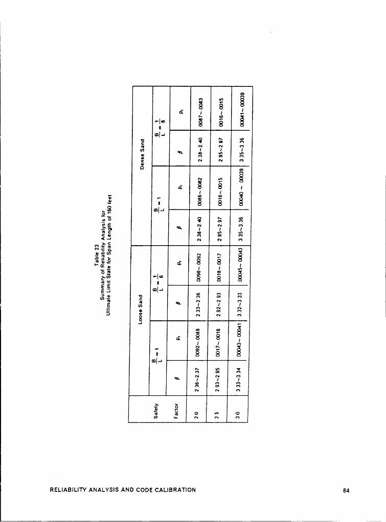
.N

Q

3 .2 2 22 2' l'“ 21** 2 2 2

m|-JE 3 3Q N 65"’ J, J,0g Z 20Q Q

" *2 ä2 2 .22 .. 2 2 g9 ¤ 8 8 .„ 3 m|.eEI.2 ° 3 «"=’»

01 C ' '22 E EC U Q C')( —‘ N n>• C

3 T; ä 2·,Q Q *0 64 r~ gg : 5 v-,2* ·· 9 8 8 2°‘ 2 2 2 J,‘ö :2 *° *:222 'L‘° 2 2 2

E EE J ‘¤I—‘M ÜDug 2 E °? *7

N N N 65E 2 J. J.ä 2 2 28J 7*

2 2 ,2I I es

¤ 88NI-JY~ M5 V*2 3 <'eN N C')2 2 2N N 65

> &

N ¢¤tf) u. ll!


SERVICEABILITY LIMIT STATE ISF:I.0

1.5

><W 1.0OZ

>·P .

..1

0<

O———--I

lu 0.5 ___.....+-——•-—-—-•-——-+-——+———+———-•-————+-———-+———-—+E ____,--A...----A--——···ab··~··--6··—····6-·····~·6-----··~6-—·-·—-6·-·----6·-------6

0.00 l 2 3 ll 5 6 7 8 9 10

DEAD/LIVE LOAD (NOMNAL) RATIO6-a—6‘3".=E.;’ITSS SCN?

E/L =l. CETQEE SCSI] +--1--+ ;.'„ =1.'E.?€‘.;; ; —

Figure 17. Reliability Index ß versus Different Dead to Live Load Ratios for Serviceability LimitState: Ratio of allowable to actual settlement -1.0


l

lSERVICEABILJTY LIMIT STA TE _

$F=!.5

LS

I

XW1.0

O

>. -„--··A·-•····A---·—-·—A-··~···45·—-~---A---.....A.......A,,,,,,_A_______A________A

P5

.1Ä

<.|lu 0.5II

0.00 1 2 3 II S 8 7 8 9 IO

DEAD/LNE LOAD (NOMINAL) RATIO5-9-6 9/L=l.LCCSE SRWC ¤·-A·~A E/L=1/€.L€C‘EE S2•—•—• E/L=l.SEN’$E SRNC 4--+-+ ER

Figure 18. Reliability Index B versus Different Dead to Live Load Ratios for Serviceability LimitState: Ratio of allowable to actual settlcment -1.5


1

SERVICEABILITY LIMIT STA TESF=2.0

IOS

’{„..•-6-···-··•4··——-4—-———Q—-··-0·-·—-4---—-4--——·4————-4--——-I

,..--4·-——•-—-——•-——·—•———-•-———+———--•-————+——-—-•-————+

.•-·-··G·•••·••A···•····A·••·•··G•••·•••G···•·••A········A·······G·······A········A><W 1.0OZ

>-P I

..I

<.ILu 0.5E

olo

Ü l 2 3 N S 6 7 8 9 IO

DEAD/LIVE LOAD (NORMAL) EATlO8-8-8 E3/L·l.l.DDSE SEND G•A·—¤ E/L=l/‘E.LDCSE SE•-•-• 9/L=l„DENSE SEND -•—+-+ E/L=l/S.DENSE SE ’

Figure 19. Reliability lndex ß versus Different Dead to Live Load Ratios for Serviceability LimitState: Ratio of allowable to actual settlement -2.0


. 1

ua an'J ZZ

I 'T 'T¤'1|-1

n n cnY °! 'T3 8 8 7~ 9 S :*2"’ c ci 60mc0

1* 1*Q v eo'T Q

,. aa vv •¤| •ä Q

c¤|-13 97 7 0·5-I., 2 23 3 2gg 6 6 : $:2 3 2<C E ¤QS 2 2 2 Q S'vz-• Q $3 •r C I°‘“>•

I · I I ‘°222 —|·¤ 3 3 Bggg u Q . •ä ¤ 2"v~„§ ·==·|· 2 2gg 2 2 2 5 2

° Y Q m §(0 'D Ö C V* Q.cevan0” Ü8 8.1 __

éI 'T¤1|-1

8 8 88 7 7c1 ca ceG G •·


l

footings on dense sand are larger than those of footing on loose sand. This ls rea-

sonable because the probability of failure for footings on dense sand should be less

than that for footings on loose sand for the same factor of safety. Rellability indlces

for square footing were slightly higher than those for long footings. This is more ev-

ident for loose sand than for dense sand and might be explained as followsz a square

footing has larger width than a long footing for the same area. Thus, a square footing

_ should have a larger bearing capacity than a long footing. The difference ls de-

creased due to a consideration of the plain straln effect for a long footing. A larger

value of friction angle ls used for long footings (see Eq. 3.12). The difference in the

friction angle between a long footing and a square footing is larger for dense sand

than for loose sand. Thus, the difference in the reliability index for a square footing

and a long footing is less for dense sand than for loose sand.

Reliability indlces vary slightly with dead to live load ratio when the dead to live load

ratio is less than 1. This is more evident for shorter spans bridges than for longer

spans bridges. lt is due to the larger bias factors shorter span bridges have than do

longer span bridges. There ls less variation in the reliability index for larger dead to

live load ratlos. The largest value of reliability index occurs at dead to live load ratio

equal to 1 for all four different span bridges. The variation of reliability index at low

dead to live load ratlos ls attributable to the larger value of overall coefficient of var-

iation for applied load. The overall coefficient of variation for applied load reaches its

smallest value at a dead to live load ratio equal to 1. When dead to live load ratio

lncreases, the dead load becomes dominant and the overall c.o.v. for applied load

approaches a constant value for all four different span bridges. The reliability index

varies more for short span bridges than for medium to long span bridges; however,

the difference ls not significant.

lV RELlABll.lTv ANAl.vsls AND CODE CALIBRATION 89l _ 2

’l

Reliability indices for serviceability limit state appear to be reasonable. The proba-

bility that the actual settlement will exceed the predicted settlement is in the range

of 0.08 to 0.33 which is in good agreement with what may be expected. It is observed

that the reliability index for footings on dense sand is higher than that for footings on

loose sand. This is in good agreement with what we know. For a footing on the same

type of soil, it is observed that a square footing has a larger reliability index than a

long footing for the same footing area. This is because a square footing has larger

footing width. lt is also found that reliability indices for serviceability limit state are

not sensitive to the dead to live load ratio.

SELECTION OF TARGET RELIABILITY INDEX

The selection of target reliability index, 6,, for each limit state with different safety

factors should be based on a measure of closeness between the code realization and

its objective. For a level ll objective, a criterion for closeness is that the expected

value of (ß, — 6)* should not exceed a given value, say 0.05, for ultimate and service-

ability limit states. Based on this procedure, the target reliability indices are selected

as ,6, = 2.3, 2.9 and 3.3 for safety factors equal to 2.0, 2.5 and 3.0 for ultimate limit

state for all span lengths. The target reliability indices for serviceability limit state

are 0.45, 0.85, and 1.1 for safety factors equal to 1.0, 1.5, and 2.0, respectively.

RELIABILITY ANALYsis AND CODE cALiBRATioN so

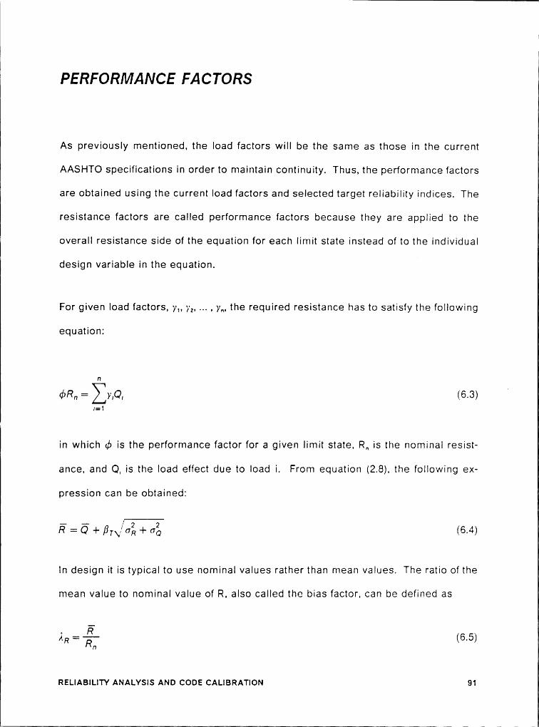
i

l

PERFORMANCE FACTORS

As previously mentioned, the load factors will be the same as those in the current

AASHTO specifications in order to maintain continuity. Thus, the performance factors

are obtained using the current load factors and selected target reliability indices. The

resistance factors are called performance factors because they are applied to the

overall resistance side of the equation for each limit state instead of to the individual

design variable in the equation.E

For given load factors, y., ya, , y„, the required resistance has to satisfy the following

equaüon:

fl

¢>Rn = Zyp, (6.3)A

/=1

in which tb is the performance factor for a given limit state, R, is the nominal resist-

ance, and Q, is the load effect due to load i. From equation (2.8), the following ex-

pression can be obtained:

ä—' ) 2 2=Q+ßT\/UR+UQln

design it is typical to use nominal values rather than mean values. The ratio of the

mean value to nominal value of R, also called the bias factor, can be defined as

. RÄ. =——· 6.5R Rn ( Ä


From equations (6.3), (6.4) and (6.5), after transformation, the performance factor can

be expressed as:

fl

ÄRZWQId)—

2 2

The dead load factor, yo, is 1.3 and the live load factor, yL, is 2.17 in current AASHTO

specifications for one ultimate limit state. For the serviceability limit state the dead

load and live load factors are both equal to 1. Figures 19 and 20 show the perform-

ance factors corresponding to the different safety factors for the ultimate and ser-

viceability limit states.

lt is observed that performance factors for the ultimate limit state almost decrease ‘

exponentially when dead to live load ratio increases. ln other words, performance

factors decrease exponentially as bridge span increases. For a given value of the

dead to live load ratio the performance factor can be obtained from Figure 20. The

performance factors for serviceability the limit state do not vary very much with dead

to live load ratio.

Thus, the ULS design criterion for dead and live load can be written as

q5R21.3><D+2.17><l. (6.7)

The relationship of performance factor gb, safety factor, and target reliability indices

for ultimate limit state is shown in Table 25.

RELIABILITY ANALYsis AND CODE cAt.lBRATloN 92

The SLS design crlterion for dead and live load with calibrated load and resistance

factors are

¢R 2 D + L (6.6)

The relationship between the performance factor eb, the traditional safety factor, and

target reliability indices for serviceability limit state ls shown in Table 26.

RELIABILITY AraA1.vsis AND CODE CALIBRATION 93

ULTIHA TE LIM]T STATE.

E‘„P

‘s\ - ‘ ; _1

< 0.6 ‘~IL \

Ä°~,

\\ ~°*•*—~•~·

Z \\ *°°°“"*"“'•·~A·•··---4< "~„·2 —‘“~•„____•

g oeu —·—_——¢—.--·-el-.°°“"•'••~~§•-~..,•

ILEIIIL

0.2

A

000

0 1 2 3 WI S B 7 0 9 l0EAU/UVE LOAD CNOKIIAL) RATD

B-B-6 SF•2.Ü ¢··A··¢ SF-2.5 I-•-• SF•3.U

Figure 20. Performance Factors for Ultlmate Llmlt State


i i

SERVICEABILITY LIM]T STATE

Ilo

0.0

O .P-

° -....< 0.8 “*··~····6··~····6--·····6·······6-·-·····6·-·····6······-6······~6---·-·-6IL

IIJOZ<2 *·—·~·~—•--——--•--—-—•--———•-———-6———--•-—-—-6-—~—-•-—-——•——---•üO

°•qIL

luIL

0.2

0 1 2 0 I S 0 7 0 9 10[EAD/LNE LOAD INONIIALJ RATIO

a—a-6 SF·1.0 6-6-6 SF·1.5 •-•-• SF-2.0

Figure 21. Performance Factors for Serviceability Limit State


Table 25. Relationship of Safety Factor, Target Reliability Index and Performance Factor for Ulti-mate Limit State

Safety Factor Target Reliability Performance FactorIndices

2.0 2.3 0.6~0.9

- 2.5 2.9 O.5~O.7

3.0 3.3 0.4~0.6

Table 26. Relationship of Ratio of Actual to Predicted Bearing Pressure, Target Reliability Indexand Performance Factor for SLS

Ratio of Actual to Target Reliability Performance FactorPredicted Bearing Pressure Indices

1.0 0.45 1.0

2.0 1.1 0.5

Rst.iAaimv Amtvsis Ann coos cAi.iammo~ 96

l

Chapter 7

CONCLUSIONS

A LFD format for the design of shallow foundations for bridges is developed in order

to provide a consistent approach to the design of the bridge superstructure and

foundations. The code calibration was performed using reliability theory. Uncer-

tainties in the design equations and design parameters for ultimate and serviceability

limit states were investigated and their statistics were obtained. Rellability indices

inherent in the current allowable stress design method for shallow foundations of

bridges were determined. Reliabillty indices for ultimate limit state are ln the range

of 2.3 to 3.4, for safety factors between 2 and 3. The corresponding probability of

failure is in the range of 10*2 to 10**. This ls in good agreement with l\/leyerhof's con-

clusions (1970). The corresponding performance factors were found to be in the

range of 0.4 to 0.9.

Reliabllity indices for serviceability limit state are in the range of 0.43 to 1.40, for the

iratlos of allowable to actual settlement between 1.0 and 2.0. The corresponding

CONCLUSIONS 97

lprobability of failure is in the range of 0.34 to 0.08. This appears to be in good

agreement with what may be expected Generally speaking, the results of the reli-

ability analyses are in good agreement with results presented by other investigators;

that is, the design of shallow foundations on sand ls controlled by settlement criteria

in almost all cases.

Reliability-based design procedures appear to be a useful tool for dealing with

geotechnical engineering problems. Although this study concentrated only on dead

and live load combinations, future extensions that include different load combinationsare possible as long as the statistics of these load combinations and suitable load

ratlos are available. This study illustrates the application of reliability-based design

to the design of shallow foundations of bridges.

CONCLUSIONS 98

Bibliography

Abdul-Baki, A. and Beik L.A., "Bearing Capacity of Foundations on Sand", Journal of SoilMechanics and Foundation Division, ASCE, Vol. 96, No. SM2 (March 1970) pp. 545-559.

Allen D.E., "Limit States Design - A Probabilistic Study", Canadian Journal of Civil Engineer-ing, Vol. 2, (1975) pp. 36-49.

Allen D.E., "Limit States Design: What do we really want?", Canadian Journal of Civil Engi-neering, Vol. 8, (1981) pp. 44-50.

American Institute of Steel Construction, Load and Resistance Factor Design Speciücation forStructural Steel Buildings, (1986) pp. 6-1 - 6-313.

Ang, A.H-S., and Tang, W.H.. Probability Concepts in Engineering Planning and Design Vol. 1,John Wiley and Sons, N.Y., N.Y., 1975.

Bieganousky, W.A., and Marcuson, W.F., lll, "Laboratory Standard Penetration Tests on FineSands", Journal of Geotechnical Engineering, ASCE, Vol. 103, No. GT6 (June 1977) pp.565-587.

Bieganousky, W.A. and Marcuson, W.F., lll, "Liquefication Potential of Dams and Foundations1 Report 1, Laboratory Standard Penetration Tests on Reid Bedford Model and OttawaSands", Research Report S-76-2, U. S. Army Engineer Watervvays Experiment Station,Vicksburg, Oct. 1976, 96 pp.

Bowles, J.E., Foundation Analysis and Design McGraw-Hill Book Co., New York, (1982) 816 pp.

Briaud, J.L. and Tucker, M., "Coefticient of Variation of In-Situ Tests in Sand". ASCE Sympo-sium on Probabilistic Characterization of Soil Properties, Atlanta, (1984) pp. 119-139.

Burland, J.B. and Burbridge„ M.C., "Settlement of Foundations on Sand and Gravel", Instn.Civ. Engrs, Part 1, Vol. 78, (Dec 1985) pp. 1325-1381.

Cornell, C.A., "Bayesian Statistical Decision Theory and Reliability-Based Design", Int. Conf.

Ä

on Structural Safety and Reliability, Washington D. C.. (1969) pp. 47-66.

Bibliography 99

l

Danish Geotechnical Institute, "Code of Practice for Foundation Engineering", 3rd Edition, DS415, Bulletin No. 36 (1985) 53 pp.

D’Appolonia D.J., D’Appolonia E. and Brissette R.F., "Settlement of Spread Footings onSand", Journal ofthe Soil Mechanics and Foundations Division, ASCE, Vol. 94, No. SM3,(May, 1968) pp.735-760.

De Beer, E.E., "Experimental Determination of the Shape Factors and the Bearing CapacityFactors of Sand", Geotechnique, Vol. 20, No. 4 (1970) pp.387-411.

Ditlevsen, O., "GeneraIized Second Moment Reliability lndex", Journal of Structural Division,ASCE, Vol. 7, No. ST4 (Apr. 1974), pp. 435-451.

Duncan J.M. and Buchighnani, A.L., An Engineering Manual for Settlement Studies, Universityof California, Berkeley, 1976, 94 pp.

Ellingwood, B., et al., "Development of a Probability·Based Load Criterion for American Na-tional Standard A58", National Bureau of Standards Special Publication No. 577, Dept. ofCommerce, Washington, D.C. (1980) 222 pp.

Ellingwood, B., et al., "Safety Checking Formats for Limit States Design", Journal of StructuralDiv., ASCE, Vol. 108, No. ST7 (July 1982) pp. 1481-1493.

Galambos T.V. et al., "ProbabiIity Based Load Criteria:Assessment of Current DesignPractice", Journal of Structural Division, ASCE, Vol. 108, No. ST5. (May 1982) pp. 959-977.

Grouni, H.N. and Nowak, A.S., "CaIibration of the Ontario Bridge Design Code 1983 Edition",Canadian Journal of Civil Engineering , Vol. 11, No. 4 (Nov. 1984) pp.760-770.

Hansen, J.B., "Foundations of Structures : General Report" , 4th International Conference ofSoil Mechanics and Foundation Engineering (1957) , Vol. 2, pp. 441-447.

Hansen, J.B., "A Revised and Extended Formula for Bearing Capacity" , Danish GeotechnicalInstitute Bulletin No. 28, Copenhagen, (1970) 21 pp.

Hasofer, A.M. and Lind, N.C., ‘°Exact and Invariant Second-Moment Code Format", Journal ofEng. Mech. Div., ASCE, Vol. 100, No. EM1 (Feb. 1974) pp. 111-121.

lngra, T.S. and Baecher, G.B., "Uncertainties in Bearing Capacity of Sand", Journal ofGeotechnical Div., ASCE, Vol. 109, No. 7 (July 1983) pp. 899-914.

Ireland, H.O., Moretto, O. and Vargas, M., "The Dynamic Penetration Test;A Standard That isNot Standardized", Geotechnique, Vol. 20. No. 2, (1970) pp. 185-192.

Kovacs, W.D., Salomone, L.A., and Yokel, F.Y., "Energy Measurement in the Standard Pene-tration Test", National Building Science Series 135, National Bureau of Standards,Washington, 1981, 73 pp.

Kovacs, W.D. and Salomone, L.A., "SPT Hammer Energy Measurement" , Journal of theGeotechnical Engineering Division., ASCE, Vol. 108, No. GT4 (April, 1982) pp.599~620.

MacGregor, J.G., "Load-and-Resistance Factor Design of Concrete Highway Bridges", Trans-portation Research Record No. 711, TRB, National Research Council, Washington, D.C.(1979) pp. 1-7.

Bibliography 100

II

I

Madsen, H.O., Krenk, S. and Lind, N.C., Methods of Structural Safety, Prentice Hall lnc., NewJersey, (1986) 403 pp.

Meyerhof, G.G., "Safety Factors and Limit States Analysis in Geotechnical Engineering",Canadian Geotechnical Journal, Vol. 21, (1984) pp. 1-7.

Meyerhof, G.G., "Safety Factors in Soil Mechanics", Canadian Geotechnical Journal, Vol. 7,(1970) pp. 349-355.

Meyerhof, G.G., "Shallow Foundations", Journal of the Soil Mechanics and Foundations Divi-sion, ASCE, Vol. 91, No. SM2, (March, 1965) pp. 21-31.

Meyerhof, G.G., "Some Recent Research on the Bearing Capacity of Foundations", CanadianGeotechnical Journal, Vol.1, No. 1, 1963.

Meyerhof, G.G., "The Ultimate Bearing Capacity of Foundations", Geotechnique, Vol. 2, (1951)pp. 301-332.

Moses, F. and Ghosn, M., "A Comprehensive Study of Bridge Loads and Reliability", FinalReport to ODOT, Civil Eng. Dept., Case Western Reserve Univ., Cleveland, (Jan. 1985) 189PD-

Nowak, A.S., "Calibration Task Group", NCHRP Project 12-33, Report No. 2, Department ofCivil Engineering, University of Michigan, Ann Arbor, Michigan, November 1989, 112 pp.

Ontario Highway Department, Ontario Highway Bridge Design Code , 2nd Edition, Ministry ofTransportation and Communication, Highway Engineering Division, Toronto, Ontario(1983) 357 pp.

Orchant, C. J., Kulhawy, F. H., and Trautmann, C. H., "ReIiability -Based Foundation Design forTransmission Line Structures", Final Report, EPRI Research Project 1493-4, Vol. 2 (Oct.1988) 166 pp.

Palacious, A., The Theory and Measurement of Energy Transfer During SPT Test Sampling,Ph.D. Thesis, University of Florida at Gainesville, Florida, 1977.

Rackwitz, R. and Fiessler, B., "Structural Reliability under Combined Random Load Se-quences", Computers and Structures, Vol. 9 (1978) pp. 489-494.

Ravindra, M.K. and Galambos, T.V., "Load and Resistance Factor Design for Steel", Journalof Structural Division, ASCE, Vol. 104, No. ST9, (Sept 1978), pp. 1337-1353.

Ravindra, M.K. and Lind, N.C., "Trends in Safety Factor Optimization". Beam and Beam Col-umns, Applied Science Publishers, Barking, Essex (1983) pp. 207-236.

Schmertmann, JH. and Palacios. A., "Energy Dynamics of SPT", Journal of Geotechnical En-gineering Division, ASCE, Vol. 105, No. GT8, (Aug 1979) pp. 909-926.

Sidi, l.D., Probabi/istic Prediction of Friction Pile Capacity , Ph.D. Thesis, University of Illinois,Urbana-Champaign, Department of Civil Engineering, 1986, 314 pp.

Simpson, B. and Groft, D.D., "An Approach to Limit State Calculations in Geotechnique",Ground Engineering, (1981) pp. 21-28.

Singh, A. and Lee, K.L., "Variability in Soil Parameters", 8th Annual Symposium of Engineer-ing Geology and Soil Engineering, Idaho, (1970) pp. 159-185.

Bibliography 101

l

lTang, W.H., "Principles of Probabilistic Characterization of Soil Properties", ASCE Symposium r

on Probabilistic Characterization of Soil Properties, Atlanta, (1984) pp. 74-89.

Tang, W.H., et al., "ProbabiIity Based Short-term Design of Soil Slope", CanadianGeotechnical Journal, Vol. 13, No. 3 (Aug 1976), pp. 210-215.

Tang, W.H., "Probabilistic Evaluation of Penetration Resistance" , Journal ofthe GeotechnicalEngineering Div., ASCE, Vol. 105, No. GT10, (Oct. 1981) pp. 1173-1189.

Terzaghi, K. and Peck, R.B., Soil Mechanics in Engineering Practice, John Wiley and Sons,New York, (1948).

Terzaghi, K., Theoretical Soil Mechanics, John Wiley & Sons, lnc., New York, (1943) 510 pp.

Turkstra, C.J., "Theory of Structural Design Decisions", Solid Mechanics Division, Universityof Waterloo, Waterloo, Ontario, Study No. 2 (1970) 124 pp.

Vanmarcke, E., On the Scale of Fluctuation of Random Functions , M.l.T. Research Report, No.79-19, April 1979.

Vanmarcke, E., "Probabilistic Modeling of Soil Profile", Journal of Geotechnical Division,ASCE, Vol. 103, No. GT 11 (Nov 1977), pp. 1227-1246.

Vanmarcke, E., Random Fields : Analysis and Synthesis , M.l.T. Press, Cambridge, MA. (1983)382 pp.

Verma, D. and Moses, F., "Bridge Reliability - Evaluation vs. Design", 5th ASCE SpecialConference on Probabilistic Methods in Civil Engineering, Blacksburg, (1988) pp. 233-236.

Wu, T.H., Potter, J.C., and Kjikstad, O., "Probabilistic Analysis of Offshore Site Exploration",Journal of Geotechnical Engineering, ASCE, Vol. 112, 1986, pp. 981-1000.

Bibliography 102

l

I

Appendix A

Experimental and Theoretical Values of NY

Experimental and Theoretical Values of NY 103

Q1

Table 27. Experimental and Theoretical Values of NY (After De Beer, 1970)

d>, Experimental N, Theoretical N,

36° 47.2 40.1

37° 52 47.4

38° 57.6 56.17

41° 91. 95

110. 11443° 133.4. 137.1

166.6. 165.645° 211.6. 200.8

283.4. 244.647** 383.4. 299.5

Experimental and Theoretical Values of NY 104

I

Appendix B

Experimental and Theoretical Values of SY

Experimental and Theoretical Values of SY 105

l

1

Table 28. Experimental and Theoretlcal Values of SY (After lngra and Baecher, 1983)

B . .No. T Experimental S, Theoretncal S,

1 0.12 1.3 0.952 0.14 1.1 0.943 0.15 0.98 0.944 0.16 0.94 0.945 0.16 ' 1.13 0.946 0.19 1 0.927 0.19 1.06 0.928 0.2 0.97 0.929 0.22 0.96 0.9110 0.24 1 0.911 0.25 1.06 0.912 0.25 1.08 0.913 0.26 0.97 0.914 0.27 1 0.8915 0.29 0.94 0.8816 0.31 0.98 0.8817 0.32 0.95 0.8718 0.32 1.04 0.8719 0.33 0.84 0.8720 0.33 1.17 0.8721 0.48 1 0.8122 0.49 0.75 0.823 0.49 0.88 0.824 0.49 1 0.825 0.49 1.06 0.826 0.49 1.1 0.827 0.49 1.12 0.828 0.68 0.98 0.7329 1 0.62 0.630 1 0.62 0.631 1 0.63 0.632 1 0.7 0.633 1 0.73 0.634 1 0.83 0.635 1 0.85 0.636 1 0.9 0.637 1 1 0.638 1 1.02 0.6

Experimental and Theoretical Values of SY 106

Appendix C

Experimental and Theoretical Values cf

Experimental and Theoretical Values cl lv 107

I

Table 29. Experimental and Theoretical Values of lv (After Ingra and Baecher, 1983)

No. tani Experimental I, Theoretical I,1 0.11 0.67 0.752 0.12 0.66 0.733 0.13 0.58 0.714 0.14 0.63 0.75 0.14 0.77 0.76 0.14 0.83 0.77 0.14 0.85 0.78 0.14 0.89 0.79 0.15 0.6 0.6810 0.16 0.57 0.6611 0.17 0.72 0.6412 0.18 0.55 0.6213 0.18 0.57 0.6214 0.18 0.71 0.6215 0.2 0.44 0.5916 0.21 0.51 0.5717 0.27 0.50 0.4818 0.27 0.55 0.4819 0.27 0.56 0.4820 0.27 0.57 0.4821 0.28 0.38 0.4722 0.29 0.39 0.4623 0.31 0.26 0.4324 0.36 0.43 0.3725 0.37 0.25 0.3626 0.38 0.21 0.3527 0.41 0.21 0.3228 0.53 0.14 0.2129 0.56 0.18 0.1930 0.57 0.19 0.1931 0.57 0.21 0.1932 0.58 0.11 0.1833 0.58 0.17 0.18

|

Experimental and Theoretical Values of lv 108

Appendix D

Experimental and Theeretical Values of NqSqdq

lExperimental and Theoretical Values ol NqSqdq 109

ll_s____

Table 30. Experimental and Theoretical Values of NqSqdq (After De Beer, 1970)

Experimental Nqsqdq Theoretical NqSqdq

1 30* 22.6 29.01 31* 25.7 33.01 32** 29.0 37.71 33* 35.2 43.01 34* 43.0 49.31 35** 54.0 56.61 36* 68.1 65.21 37* 89.0 75.330* 16.3 20.2l 31* 18.4 22.76é 32* 21.0 25.6

33* 25.0 28.934* 30.2 32.735* 37.7 42.3

% 36* 47.4 42.3—é— 47* 60.7 48.3

I

Experimental and Theoretical Values of NqSqdq 110

load and resistance factor design of shallow

Documents