lmdz physical schemes. a brief description for the lmdz-b ... · text of this document is partially...
TRANSCRIPT

LMDZ physical schemes. A brief description for the LMDZ-B
configuration
L. Fita
Laboratorie de Meteorologie Dynamique, IPSL, UPMC, CNRS, Tw. 45-55 3rd fl., B99, Jussieu,75005, Paris, France
August 22, 2013
Contents
1 Introduction 2
2 Radiation scheme 2
3 PBL, convection and cumulus schemes 33.1 Planetary Boundary Layer scheme . . . . . . . . . . . . . . . . . . . . . . . . . . . . . . . . . . . . . . 5
3.1.1 Thermal . . . . . . . . . . . . . . . . . . . . . . . . . . . . . . . . . . . . . . . . . . . . . . . . . 53.1.2 Cold pools . . . . . . . . . . . . . . . . . . . . . . . . . . . . . . . . . . . . . . . . . . . . . . . 6
3.2 Deep convection . . . . . . . . . . . . . . . . . . . . . . . . . . . . . . . . . . . . . . . . . . . . . . . . 73.3 Cumulus scheme . . . . . . . . . . . . . . . . . . . . . . . . . . . . . . . . . . . . . . . . . . . . . . . . 8
4 Micro-Physics scheme 9
5 Land scheme 95.1 SVAT SECHIBA . . . . . . . . . . . . . . . . . . . . . . . . . . . . . . . . . . . . . . . . . . . . . . . . 10
5.1.1 Bulk aerodynamic method . . . . . . . . . . . . . . . . . . . . . . . . . . . . . . . . . . . . . . . 125.2 Orchidee . . . . . . . . . . . . . . . . . . . . . . . . . . . . . . . . . . . . . . . . . . . . . . . . . . . . . 13
6 Others 136.1 Subgrid-scale orography . . . . . . . . . . . . . . . . . . . . . . . . . . . . . . . . . . . . . . . . . . . . 13
7 Configuration 157.1 run.def . . . . . . . . . . . . . . . . . . . . . . . . . . . . . . . . . . . . . . . . . . . . . . . . . . . . . . 157.2 config.def . . . . . . . . . . . . . . . . . . . . . . . . . . . . . . . . . . . . . . . . . . . . . . . . . . . . 167.3 gcm.def . . . . . . . . . . . . . . . . . . . . . . . . . . . . . . . . . . . . . . . . . . . . . . . . . . . . . 187.4 physiq.def . . . . . . . . . . . . . . . . . . . . . . . . . . . . . . . . . . . . . . . . . . . . . . . . . . . . 197.5 traceur.def . . . . . . . . . . . . . . . . . . . . . . . . . . . . . . . . . . . . . . . . . . . . . . . . . . . . 207.6 orchidee.def . . . . . . . . . . . . . . . . . . . . . . . . . . . . . . . . . . . . . . . . . . . . . . . . . . . 21
error Value needed explanation needed doubt
1

'
&
$
%
LMDZ -�
6���� ���� ���� ����?
Turbulence−convective
PBL
thermalsconvectioncold poolscumulus
Micro-Physics
Land
Radiation
sub-scale orography
output
startfi, histfistatisticsdump. eofdiagfi
?
Figure 1: Schematic representation of the physics schemes used by LMDZ
1 Introduction
This document attempts to be a short introduction to the series of schemes that constitute the physical core ofthe Laboratoire de Meteorologie Dynamique Zoomed (LMDZ, http://lmdz.lmd.jussieu.fr/) model, developed bythe Laboratoire de Meteorologie Dynamique (LMD, http://www.ipsl.fr/en/Organisation/IPSL-Labs/LMD), of theInstitute Pierre Simone Laplace (IPSL, http://www.ipsl.fr/en) of the Centre national de la recherche scientifique(CNRS, http://www.cnrs.fr/).
The schemes are basically developed initially by 1D case study simulations and re-tunned for the 3D runs.Text of this document is partially taken directly (as it is) from the cited articles. Due to the large amount of
this kind of text, no distinction with respect author’s original one is done. This document describes the physicalconfiguration of LMDZ known as LMDZ-B [HGR+13]
2 Radiation scheme
Radative scheme in LMDZ is an adapted version from [Mor91]. At the time of this document is being written, LMDteam is working to implement the rrtm scheme (version? rrtm, rrtmg?)
Are there in LMDZ independent vertical layers used for the radiation scheme, or does it use the same ones of themodel vertical discretization?
How does LMDZ incorporate the time-evolution of GHG gases? How does it deal with different scenarios?Is the outputted cloud fraction the same one ’used’ by the radiative scheme?Radiation scheme has suffered different evolutions from a first one (of 1979, EC1) with the interaction between line
absorption and scattering using a photon path distribution method to the last version (1989, C3, the implementedone) summarized in table 1
The transmission functions τ are computed with the help of an empirical function [Gel77] for the reduced (ur) andunreduced (u) amounts of absorbers (CO2, CH4, N2O, CO and CO2):
− ln τ =au√
1 + bu2/ur)+ cur (1)
2

where cur, continuum absorption, coefficients a, b and c incorporate the temperature dependence of the absorption(linearly dependent on 1/T) fitted to the experimental data from [MFS+72, Vig53].
Last version of the scheme has evolved from narrow-band models to high spectral resolution (225 spectral intervalsin the longwave, 208 in the shortwave) ones. Which have been compared to line-by-line calculations [SC81] and insitu measurements. These detailed models were then degraded by introducing simplifying assumptions, making themmore computationally efficient. In that process, the sensitivity of the outputs (fluxes and heating/cooling rates) tothe various assumptions have been monitored [MF85, MF86]. In the longwave, those studies showed that one of thecauses for major systematic errors is the use of wide spectral intervals which tend to overestimate the effects of thestrong lines, thus giving a poor representation of the temperature and pressure dependence of the absorption.
Clear-sky longwave fluxes are evaluated with an emissivity method incorporating a parameterization giving acorrect representation of the temperature and pressure dependence of the absorption [MSF86]. Clouds are introducedas gray bodies with a longwave emissivity depending on the cloud liquid water path, following [Ste78].
Shortwave fluxes are computed using a photon path distribution method to separate the contributions of scatteringand absorption processes to the radiative transfer. Scattering is treated with a delta-Eddington approximation.Transmission functions are developed as Pade approximates. Coefficients for the molecular absorption are calculatedfrom the 1982 version of the Air Force Geophysics Laboratory (AFGL) line parameters compilation. Cloud shortwaveradiative parameters are the optical thickness and single-scattering albedo linked to the cloud liquid water path, anda prescribed asymmetry factor [Fou88]. In EC3 a distinction is made between various cloud types by defining theoptical thickness as a function not only of the liquid water path in the cloud, but also of the effective radius are reof the cloud particles, with re varying with height from 5 µm in the planetary boundary layer to 40 µm at 100 hPa.This last feature is an empirical attempt at dealing with the variation of cloud type with height, as smaller waterdroplets are observed in low-level stratiform clouds, whereas larger particles are found in cumuliform and cirriformclouds. This radiation scheme has already been extensively tested in the ECMWF model [Mor90] and was introducedin the operational forecast model on May 2, 1989.
3 PBL, convection and cumulus schemes
In LMDZ a big effort in the turbulent and convection physics of the model has been done. Previous version of themodel [known as LMDZ-A HFC+13] used the Mellor-Yamada pbl scheme [MY74] in combination with Emanuel’sconvective one [Ema93]. In a new set of physics schemes [LMDZ-B HGR+13] huge modifications have been introducedand in this version (LMDZ v5): on the PBL scheme ’Thermals’ are tacking into account [HCM02], a new schemerepresenting cold pools due to precipitating water evaporation (wakes) have been included [GL09] which at the sametime a new closure methodology has been introduced in Emanuel’s convection [based on sub-clouds processes GPT04].All these schemes interact among each other. By this reason, in LMDZ-B there is not such split of three specificschemes (pbl, deep convection and cumulus) such in other models.
All these changes have been reported with a huge positive impact. For example, a better representation of the lowlevel clouds is attained, the daily cycle of precipitation over continents presents a maximum closer to the afternoonfixing a well known bias of the models [see HGR+13].
Semi-detailed explanation of the schemes will be done following the same scheme as in [HFC+13].The new set of parameterizations relies on the separation of three distinct scales for the turbulent and convective
subgrid-scale vertical motions:
1. The small scale (10100 m), associated with random turbulence, dominant in particular in the surface layer.
2. The boundary layer height (500 m-3 km) that corresponds to the vertical scale of organized structures of theconvective boundary layer.
3. The deep convection depth (1020 km) of cumulonimbus, meso-scale convective systems or squall lines.
The first two scales dominate the vertical subgrid-scale transport in the boundary layer. In the ’B physics’, theparameterization of this vertical transport relies on the combination of a diffusion scheme for small scale turbulenceand a mass-flux model of the organized structures of the convective boundary layer, the so-called [’thermal plumemodel’ HCM02, RH08].
3

Table 1: Summary of ECMWF radiative scheme characteristics for clear/covered sky and short/longwave spectrum
Sky wave characteristic methodClear sky
shortwave a
Rayleigh scattering Parametric expression of the Rayleighoptical thickness
Aerosol scattering and ab-sorption
Mie parameters for five types ofaerosols based on climatological models[WMO84]
Gas absorption From AFGL 1982 compilation of lineparameters
H2O One intervalUniformly mixed gasesb One intervalO3 Two intervals
longwave c
H2O Six spectral intervals, e- and p-typecontinuum absorption included be-tween 350 and 1250 cm−1
CO2 Overlap between 500 and 1250 cm−1
in three intervals by multiplication oftransmission
O3 Overlap between 970 and 1110 cm−1
Aerosols Absorption effects using an emissivityformulation
Cloudy sky
shortwave
Droplet absorption andscattering
Employs a delta-Eddington methodwith τ and w determined from LWP,and preset g and re
Gas absorption Included separately throughout thephoton path distribution method
longwave
scattering NeglectedDroplet absorption from LWP using an emissivity formula-
tionGas absorption As for clear sky, longwave above
atwo-stream formulation is employed together with photon path distribution method [FB80] in two spectral intervals (0.25-0.68 &0.68-4.0 µm)
bCO2, CH4, N2O, CO and O2cBroad-band flux emissivity method with six intervals covering the spectrum between zero and 2620 cm−1. Temperature and pressure
dependence of absorption following [MSF86]. Absorption coefficients fitted from AFGL 1982.
4

3.1 Planetary Boundary Layer scheme
Main characteristics combination of a:
• eddy diffusion
• ’thermal plume model’: mass-flux representation of the organized thermal structures of the convective boundarylayer
The boundary layer parameterization now relies on the combination of a classical eddy diffusion [Yam83] with amass-flux representation of the organized thermal structures of the convective boundary layer, the so-called [’thermalplume model’ HCM02, RH08]. It enables one to represent the upward convective transport in the mixed layer althoughthis layer is generally marginally stable [HCM02], solving a long recognized limitation of eddy diffusion [Dea66].Mass-flux schemes account reasonably well for the organized structures (thermal plumes, or rolls) of the convectiveboundary layer. Their properties are used in the new model version for coupling with deep convection and also tobetter parameterize the boundary layer clouds [RH08, JHRC11].
The computation of the eddy diffusivity Kz is based on a prognostic equation for the turbulent kinetic energy,according to [Yam83]. It is mainly active in practice in the surface boundary layer, typically in the first few hundredmeters above surface.
The mass flux scheme represents an ensemble of coherent ascending thermal plumes in the grid cell as a meanplume. A model column is separated in two parts: the thermal plume and its environment. The vertical mass fluxin the plume fth = ραthwth (where ρ is the air density, wth the vertical velocity in the plume and αth its fractionalcoverage) varies vertically as a function of lateral entrainment eth (from environment to the plume) and detrainmentdth (from the plume to the environment):
∂fth∂z
= eth − dth (2)
For a scalar quantity q (total water, potential temperature, chemical species, aerosols), the vertical transport by thethermal plume (assuming stationarity) reads:
∂fthqth∂z
= ethq − dthqth (3)
qth being the concentration of q inside the plume (air is assumed to enter the plume with the concentration of thelarge scale, which is equivalent to neglect the plume fraction αth in this part of the computation). The time evolutionof q finally reads:
∂q
∂t= −1
ρ
∂ρw′q′
∂z(4)
with
ρw′q′ = fth (qth − q)− ρKz∂q
∂z(5)
The vertical velocity wth in the plume is driven by the plume buoyancy g(θth−θ)/θ. The thermal plume fraction is alsoan internal variable of the model. The computation of wth, αth, eth and dth is a critical part of the code. Detailed testson two different versions of the eth and dth computation are presented in detail by [RH08] and [RHCJ10] respectively.
3.1.1 Thermal
Let us consider a vertical profile of potential temperature typical of the Convective Boundary Layer (CBL), with anunstable surface layer (SL) of height zs, a neutral mixed layer (ML) topped by a stable atmosphere (entrainment zoneplus free atmosphere) as shown in Fig. 2. Although the entrainment layer may or may not be an inversion layer, wewill use the classical notation zi for the height of the top of the mixed layer [following chapter 1 Stu88].
In this idealized environment, the thermal is introduced as a simple plume of buoyant air coming from the SL.Buoyancy is expressed as the gravity times the relative difference between virtual potential temperature inside andaround the thermal plume. The virtual potential temperature is
θv = T
(p0
p
)κ(1 + 0.61q) (6)
5

Figure 2: Schematic representation of a thermal from [HCM02]
where T is the air temperature, p0 = 105 Pa, κ = 0.287, and q is the specific humidity in kgkg−1. In this section, inorder to avoid the use of multiple indices, the virtual potential temperature is notified θ.
If the plume does not mix with its environment, its virtual potential temperature is that of the SL, θSL. If, inaddition, the thermal is assumed to be stationary and frictionless, the vertical velocity inside the plume, in absence ofphase change of water, is given by
dw
dt= w
∂w
∂z= g
θSL − θML
θML(7)
(horizontal pressure differences between the plume and its environment are neglected). The air is uniformlyaccelerated in the ML until the level where the mean potential temperature θ(z) exceeds θSL. This level will beretained for definition of zi. At this level, the square of the vertical velocity wmax obtained by vertically integratingEq. 7 over the depth of the CBL is twice the convective available potential energy (CAPE) defined as
CAPE =∫ zi
0
dz gθSL − θML
θML(8)
Above zi, w is still positive (overshooting) but decreases to finally vanish at the height zt (top), where∫ zt
0
dz gθSL − θ
θ= 0. (9)
The integral corresponds to the shaded area on the left-hand side of Fig. 2 and the CAPE to that part of theintegral below zi. After reaching zt, air parcels coming from the plume are heavier than the environment and shouldsink again. This will not be considered here.
What is required for transport computations is not the vertical velocity but rather the mass flux per unit area,f = αρw, where α is the fraction of the horizontal surface covered by ascending plumes and ρ is the air density. As afirst step, we assume that f is constant within the ML (no detrainment). In order to determine this constant value,it is necessary to invoke the geometry of the thermal cell. Results will depend on geometry of the plume [for furtherdetails see HCM02].
3.1.2 Cold pools
The wake model is fully described in [GL09, GLC09]. Only a short descriptive view of the scheme is presented here.The model represents a population of identical circular cold pools (the wakes) with vertical frontiers over an infinite
plane containing the grid cell. The wakes are cooled by the convective precipitating downdrafts, while the air outsidethe wakes feeds the convective saturated drafts (see figure 3).
6

Figure 3: Schematic representation of a wake from [GL09]
The wake centers are assumed statistically distributed with a uniform spatial density Dwk. The wake state variablesare their fractional coverage σw(σw = Dwkπr2, where r is the wake radius), the potential temperature difference δθ(p)and the specific humidity difference δqv(p) between the wake region (w) and the off-wake region (x). δθ(p) and δqv(p)are non zero up to the homogeneity level ph = 0.6ps (where ps is the surface pressure). Above ph the sole differencebetween (w) and (x) regions lies in the convective drafts (saturated drafts in (x) and unsaturated ones in (w)).
Wake air being denser than off-wake air, wakes spread as density currents, inducing a vertical velocity differenceδw(p) between regions (w) and (x) (δw(p) > 0). The vertical profile δw(p) is imposed piecewise linear. Especially,between surface and wake top (the altitude hw where δθ crosses zero) the slope corresponds to wake spreading withoutlateral entrainment nor detrainment.
The wake geometrical changes with time are due to the spread, split, decay and coalescence of the wakes. Split,decay and coalescence are merely represented by imposing a constant density Dwk and by assuming that when σwreaches a maximum allowed value (= 0.5) some wakes vanish (i.e. mix with the environment) while others split sothat the fractional cover σw stays constant. The spreading rate of the wake fractional area σw reads:
∂tσw = 2C∗√πDwkσw (10)
where C∗, the mean spread speed of the wake leading edges, is proportional to the square root of the WAke Poten-tial Energy WAPE: C∗ = κ∗
√2WAPE and WAPE = −g
∫ hw
0δθv
θvdz, where, κ∗, the spread efficiency, is a tunable
parameter in the range 1/3− 2/3 and θv is the virtual potential temperature.The energy and water vapor equations are expressed at each level yielding prognostic equations for δθ(p) and δqv(p)
as well as contributions to the average temperature θ and average humidity qv equations.The convective scheme is supposed to provide separately the apparent heat sources due to saturated drafts and to
unsaturated drafts, which makes it possible to compute the differential heating and moistening feeding the wakes.There are not interactions among weaks?
3.2 Deep convection
Main characteristics as combination of:
• Emanuel’s scheme
• New closure: sub-cloud processes: ALE, CIN, ALP from ’thermal plume model’ and cold pool parameterizations
7

[Ema91] convection scheme is the base for the deep convection in LMDZ, but with a modification in its closuremethodology based on the sub-cloud processes. The coupling of the convective parameterization with those of sub-cloud processes is done through the notions of Available Lifting Energy (ALE, which must overcome the ConvectiveINhibition, or CIN, for triggering) and Available Lifting Power (ALP) that controls the convective closure. Bothquantities are computed from internal variables of the ’thermal plume model’ and of a new parameterization of thecold pools created by re-evaporation of convective rainfall in the sub-cloud layer [GL09, GLC09].
This version uses the buoyancy sorting mass-flux scheme of [Ema93], with modified mixing [GPT04] and splittingof the tendencies due to saturated and unsaturated drafts. The precipitation efficiency is computed as a function ofthe in-cloud condensed water and temperature following [EuR99]. It is bounded by a maximum value epmax which isslightly less than unity to allow some cloud water to remain in suspension in the atmosphere instead of being entirelyrained out [BE01].
The ALE allows to overcome the Convective INhibition (CIN) so that convection is triggered when ALE > |CIN |.The closure consists in prescribing the mass flux M at the top of the inhibition zone as:
M =ALP
2w2B + |CIN |
(11)
where wB is the updraft speed at the level of free convection. The original constant value wB = 1m/s was replacedby a function of the level of free convection as explained below.
In this version, two processes are taken into account for both ALE and ALP: (1) the ascending motions of theconvective boundary layer, as predicted by the thermal plume model and (2) the air lifted downstream of gust fronts.ALE is the largest of the lifting energies provided by the two processes: ALE = max(ALEth, ALEwk) where ALEthscales with w2
th and ALEwk = WAPE (see eq. 10). ALP is the sum of the lifting powers provided by the twoprocesses: ALP = ALPth +ALPwk where ALPth scales with w3
th and ALPwk scales with C3∗ (see eq. 10).This coupling between cold pools (generated by convection) and convection (triggered in turn and fed by cold
pools) allows for the first time to get an autonomous life cycle of convection, not directly driven by the large scaleconditions.
3.3 Cumulus scheme
It is based on a bi-gaussian statistical cloud scheme (Jam et al., 2011) This article does not exist!!The fractional cloudiness αc and condensed water qc are predicted by introducing a subrid-scale distribution P (q)
of total water q so that:
αc =∫ ∞qsat
dq P (q) (12)
qc =∫ ∞qsat
(dq q − qsat)P (q) (13)
where qsat(T ) is the grid averaged saturation specific humidity in the mesh.For deep convection (see scheme in figure 4), we assume that the subgrid-scale condensation and rainfall can be
handled by the Emanuel scheme, so that this statistical cloud scheme is used only to predict the fractional cloudinessfor the radiative transfer. Following [BE01], the in-cloud water (qinc = qc/αc) predicted by the convective scheme isused, through an inverse procedure, to determine the variance σ of a generalized log-normal function bounded at 0.With this particular function, the skewness of P (q) increases with increasing values of the unique width parameterξ = σ/q.
For other types of clouds, the statistical cloud scheme is used to compute not only the cloud properties for radiationbut also ’large scale’ condensation.
If the thermal plume is not active in the grid box (in practice if fth = 0 see equation 2), the width parameter ξ ofthe generalized log-normal function is specified as a function of pressure: ξ(p) increases linearly from 0 at surface toξ600 = 0.002 at 600 hPa, then to ξ300 = 0.25 at 300 Pa. It is kept constant above.
When fth > 0 in the grid box, two options are available. Either we use the [BE01] procedure to invert the widthparameter ξ from the knowledge of the condensed water computed in the thermal plumes (like what is done for deepconvection) or we use a new statistical cloud scheme proposed by [JHRC11] in which the sub-grid scale distributionof the water saturation deficit (rather than total water) is parameterized as the sum of two Gaussian functions,
8

representing the variability within and outside the thermal plume respectively. The width of each Gaussian varies asa function of the thermal plume fractional cover αth and of the contrast in saturation deficit between the plume andits environment.
A fraction fiw of the condensed water qc is assumed to be frozen. This fraction varies as a function of temperaturefrom fiw = 0 at 273.15 K to fiw = 1 at 258.15 K. The condensed water is partially precipitated. Derived from [ZK97]formula for an anvil model, the associated sink is
dqiwdt
=1ρ
∂
∂z(ρwiwqiw) (14)
where wiw = γiw × w0, w0 = 3.29(ρqiw)0.16 being a characteristic free fall velocity (in m/s) of ice crystals given by[HD90] and γiw a parameter introduced for the purposes of model tuning (ρ in kg/m3).
For liquid water, following [Sun78], rainfall starts to precipitate above a critical value clw (0.6 g/kg in the referenceversion) for condensed water, with a time constant for auto-conversion τconvers (= 1, 800 s) so that
dqlwdt
= − qlwτconvers
[1− e−(qlw/clw)2
](15)
A fraction of the precipitation is re-evaporated in the layer below and added to the total water of this layer beforethe statistical cloud scheme is applied. For ice particles, we assume that all the precipitation re-evaporates. For liquidwater, following [Sun88], we assume that
∂P
∂z= β [1− q/qsat]
√P (16)
where P is the precipitation flux, and β a tunable parameter.The effective radius of cloud droplets depends on the aerosol concentration which is specified as a function of space
and season as explained by [DFD+13] this issue. The effective radius of ice crystals varies linearly as a function oftemperature between eriw,max at 0 ◦C and eriw,min at −84.1 ◦C.
The second point concerns the treatment of stratocumulus. Although some encouraging work is done currentlyon the thermal plume model in that direction, the current version does not represent properly strato-cumulus clouds.Strato-cumulus are known to be especially prominent at the eastern side of tropical oceans. On the other hand, the[Yam83] scheme alone performs quite well for those particular conditions. A kludge is thus introduced in the model,which consists in identifying the atmospheric columns with a sharp temperature inversion at the boundary layer top,and turning off the thermal plume model in those particular cases. In practice, if
T∂θ
θ∂p< −0.08K/Pa (17)
then the thermal plume parametrization is arbitrarily switched off. This test is in fact inherited from the standardLMDZ5 model where it was used to switch between two different computations of the Kz coefficient with the samegoal of contrasting the regions of strato-cumulus and trade wind cumulus on tropical oceans.
4 Micro-Physics scheme
No microphysics scheme is set up in LMDZ.Meaning that no water species (drops,
←−−−−−−−−−−−−−−−−−−−−−−−−−−−−−−−−→ice↔ liquid↔ vapor, graupel, snow, supercooled water,...) dynamics can
occur in the LMDZ modelLook in WRF which is the simplest optionWhat about diabatic processes inside the plume and wake schemes?
5 Land scheme
What if Orchideee is not set up? SVAT SECHIBA?
9

Cumulus
Deepconvection
: Emanuel + sub− cloud closure
other : statistical, ξ
{Emanuel(PDFinside + PDFoutside) |H2O sat. deficit
plume active
lin. up to 0.002 p ≥ 600 hPalin. up to 0.25 600 hPa > p ≥ 300 hPact. 0.25 p < 300 hPa
plume inactive
Strato−cumulus : huge T∂θ
θ∂p Switch off plume
Figure 4: Schematic representation of the diagram flow for the cumulus parameterization
Figure 5: Example of water balance (Amazonian) for a given precipitation amount and the respective percentagesfrom measured values [first, bold Shu88] and simulated [second, italic SSR+89] from [DLP93]
5.1 SVAT SECHIBA
Surface-vegetation-atmosphere transfer (SVAT) SECHIBA [DLP93, dRP98] has been developed as a set of surfaceparameterizations for the LMDZ. SVAT simulate exchanges of sensible, latent and kinetic energy at the surface.SECHIBA describes exchanges of energy and water between the atmosphere and the biosphere, and the soil wa-ter budget. In its standard version, SECHIBA contains no parameterization of photosynthesis. Time step of thehydrological module is of the order of 30 min.
For each grid point eight land surface types (bare soil plus seven vegetation classes) are defined, each of themcovering a fractional area of the grid box and allowed to be found simultaneously. Over each of these covers thetransfers are computed: evaporation from soil, transpiration from plants through a resistance defined by concepts ofstomatal resistance and architectural resistance, and interception loss from the water reservoir over the canopy (see anschematic representation in figure 5). These fluxes are then averaged over the period box to derive the total amountof water vapor that is transferred to the first level of the atmospheric model. Parameterization of soil water allowsfor the moistening of an upper layer, of variable depth, during a rainfall event. The scheme requires prescription of arestricted number of parameters: seven for each class of vegetation not found and four for the soil not found.
SECHIBA represents:
• latent heat flux: exchanges of water vapor between the soil/vegetation system and the atmosphere
• soil hydrological cycle
10

Table 2: Equations for each element of the latent heat flux decomposition from [DLP93]∆q α
∑` r`
Snow sublimation qsat(Tg)− qa Sn
Scrra
Soil evaporation hgqsat(Tg)− qa(
1− Sn
Scr
)(1− σf ) ra + rg
Canopy transpiration hgqsat(Tg)− qa(
1− Sn
Scr
)σf
(1−
(Wdew
Wdmax
)2/3)
ra + r0 + rc
Evaporation of foliage water qsat(Tg)− qa(
1− Sn
Scr
)σf
(Wdew
Wdmax
)2/3
ra + r0
Table 3: Canopy parameters prescribed in SECHIBA
Parameters Tundra GrasslandGrassland
+ shrub cover
Grassland
+ tree cover
Decidius
forest
Evergreen
forestRain forest
LAI Summer 1 2 2.5 3.5 5 4 8LAI Winter 0 1.5 1 1.5 0 3 8r0 (sm−1) 10 2 2.5 3 40 50 25k0 (kgm−2s−1 10−5) 5.0 30.0 25.0 28.0 25.0 12.0 24.0
Vegetation is treated as a single element in the equations. However, because different fractions of vegetationtypes can coexist in the grid box, certain vegetation contributions such as evapotranspiration will be the result of thecombination of all the classes of vegetation within the grid box.
For sensible heat flux calculations vegetation and soil are considered as a single element.Total latent heat flux (Ea) would be the weighted combination of snow sublimination (Es), soil evaporation (Eg),
canopy transpiration (Etr) and evaporation of foliage water (Ei, intercepted precipitation and dew). Each of one iscomputed following:
Es,g,tr,i = αs,g,tr,iρ∆qs,g,tr,i∑
` r`(18)
where ∆qs,g,tr,i is the gradient of specific humidity between the evaporating surface and the overlying air, and limitedby a sum of resistances (r`). αs,g,tr,i is the fraction of grid box evaporating and ρ air density. This formulation wasintroduced by [Mon63] and is known by the ’big-leaf’ or ’single-leaf’ model.
There is an aerodynamic resistence (ra) that opposes the transfer of water vapor which is inversely proportional tothe product of the surface drag coefficient (Cd) and the wind speed (Va).
ra =1
CdVa(19)
Soil evaporation is calculated following a bulk aerodynamic method (see section 5.1.1) as a combination of thesurface relative humidity (hg) and a soil resistance (rg, see equation 20) which are function of the soil moisture. Soilresistance has a dependency on the soil type tacking its values from observations [Mat83b, Mat83a, Mat84].
rg = rsoilDu
Dt
Wumax −Wu
Wumax(20)
The architectural resistance (r0) would take into account the aerodynamic resistance between leaves and canopy top.In this scheme canopy is defined as a single layer, and a resistance is included following [SK91]. Values are taken froma Perrier (personal communication) and are function of the vegetation type (see table 3)
The canopy resistance (rc, see equation 21) summarizes the bulk stomatal and leaf aerodynamical resistances. Itdepends on the solar radiation (Rs) and the water vapor concentration deficit (δc) simulated above canopy being
11
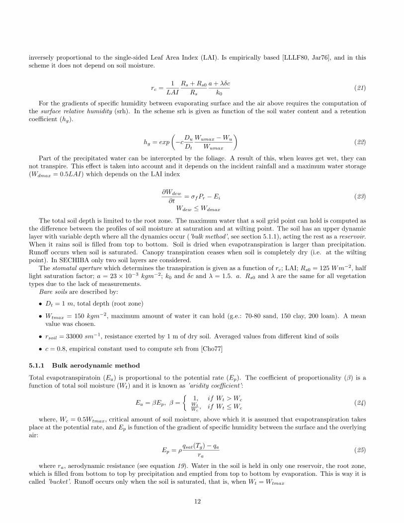
inversely proportional to the single-sided Leaf Area Index (LAI). Is empirically based [LLLF80, Jar76], and in thisscheme it does not depend on soil moisture.
rc =1
LAI
Rs +Rs0Rs
a+ λδc
k0(21)
For the gradients of specific humidity between evaporating surface and the air above requires the computation ofthe surface relative humidity (srh). In the scheme srh is given as function of the soil water content and a retentioncoefficient (hg).
hg = exp
(−cDu
Dt
Wumax −Wu
Wumax
)(22)
Part of the precipitated water can be intercepted by the foliage. A result of this, when leaves get wet, they cannot transpire. This effect is taken into account and it depends on the incident rainfall and a maximum water storage(Wdmax = 0.5LAI) which depends on the LAI index
∂Wdew
∂t= σfPr − Ei (23)
Wdew ≤Wdmax
The total soil depth is limited to the root zone. The maximum water that a soil grid point can hold is computed asthe difference between the profiles of soil moisture at saturation and at wilting point. The soil has an upper dynamiclayer with variable depth where all the dynamics occur (’bulk method’, see section 5.1.1), acting the rest as a reservoir.When it rains soil is filled from top to bottom. Soil is dried when evapotranspiration is larger than precipitation.Runoff occurs when soil is saturated. Canopy transpiration ceases when soil is completely dry (i.e. at the wiltingpoint). In SECHIBA only two soil layers are considered.
The stomatal aperture which determines the transpiration is given as a function of rc; LAI; Rs0 = 125 Wm−2, halflight saturation factor; a = 23 × 10−3 kgm−2; k0 and δc and λ = 1.5. a. Rs0 and λ are the same for all vegetationtypes due to the lack of measurements.
Bare soils are described by:
• Dt = 1 m, total depth (root zone)
• Wtmax = 150 kgm−2, maximum amount of water it can hold (g.e.: 70-80 sand, 150 clay, 200 loam). A meanvalue was chosen.
• rsoil = 33000 sm−1, resistance exerted by 1 m of dry soil. Averaged values from different kind of soils
• c = 0.8, empirical constant used to compute srh from [Cho77]
5.1.1 Bulk aerodynamic method
Total evapotranspiratoin (Ea) is proportional to the potential rate (Ep). The coefficient of proportionality (β) is afunction of total soil moisture (Wt) and it is known as ’aridity coefficient’:
Ea = βEp, β ={
1, if Wt > WcWt
Wc, if Wt ≤Wc
(24)
where, Wc = 0.5Wtmax, critical amount of soil moisture, above which it is assumed that evapotranspiration takesplace at the potential rate, and Ep is function of the gradient of specific humidity between the surface and the overlyingair:
Ep = ρqsat(Tg)− qa
ra(25)
where ra, aerodynamic resistance (see equation 19). Water in the soil is held in only one reservoir, the root zone,which is filled from bottom to top by precipitation and emptied from top to bottom by evaporation. This is way it iscalled ’bucket’. Runoff occurs only when the soil is saturated, that is, when Wt = Wtmax
12

Figure 6: Schematic representation of the drag introduced by a mountain from [LM97]
5.2 Orchidee
Orchidee (http://orchidee.ipsl.jussieu.fr/) [KVdND+05] is a dynamic global vegetation model designed asan extension of an existing surface-vegetation-atmosphere transfer scheme which is included in a coupled ocean-atmosphere general circulation model. The dynamic global vegetation model simulates the principal processes of thecontinental biosphere influencing the global carbon cycle (photosynthesis, autotrophic and heterotrophic respirationof plants and in soils, fire, etc.) as well as latent, sensible, and kinetic energy exchanges at the surface of soilsand plants. As a dynamic vegetation model, it explicitly represents competitive processes such as light competition,sampling establishment, etc. It can thus be used in simulations for the study of feedbacks between transient climateand vegetation cover changes, but it can also be used with a prescribed vegetation distribution. The whole seasonalphenological cycle is prognostically calculated without any prescribed dates or use of satellite data. Orchidee is basedin three components:
• SVAT ESCHIBA [DLP93, dRP98] for the basics interchanges between atmosphere and soil
• Dynamic Global Vegetation Model (DGVM LPJ) [SSP+03] for the vegetation dynamics
• Saclay Toulouse Orsay Model for the Analysis of Terrestrial Ecosystems (STOMATE) based in plant functionaltypes (PFT) for photosynthesis, carbon allocation, litter decomposition, soil carbon dynamics, maintenance andgrowth respiration and phenology
6 Others
6.1 Subgrid-scale orography
Effects of subgrid-scale orography (SSO) are accounted for both through drag and lifting effects on the obstacles andthrough generation and propagation in the atmosphere of gravity waves [LM97].
The assumption is that the mesoscale flow dynamics can be described by two conceptual models, whose relevancedepends on the non-dimensional height of the mountain, viz.
Hn =NH
|U |(26)
where H is the maximum height of the obstacle, U is the wind speed and N is the Brunt-Vaisala frequency of theincident flow (see figure 6).
At small Hn, all the flow goes over the mountain and gravity waves are forced by the vertical motion of thefluid. Suppose that the mountain has an elliptical shape and a height variation determined by a parameter b in thealong-ridge direction and by a parameter a in the cross-ridge direction, such that
γ = a/b ≤ 1 (27)
then the geometry of the mountain can be written in the form
h(x, y) =H
1 + x2/a2 + y2/b2(28)
13

In the simple case when the incident flow is at right angles to the ridge the surface stress due to the gravity wave hasthe magnitude
τw = ρ0bGB(γ)NUH2 (29)
provided that the Boussinesq and hydrostatic approximations apply. In Eq. 29 G is a function of the mountainsharpness [Phi84], and for the mountain given by Eq. 28, G ≈ 1.23. The term B(γ) is a function of the mountainanisotropy, γ, and can vary from B(0) = 1 for a two-dimensional ridge to B(1) = π/4 for a circular mountain.
At large Hn the vertical motion of the fluid is limited and part of the low-level flow goes around the mountain.The depth, Zb, of this blocked layer, when U and N are independent of height, can be expressed as
Zb = Hmax
(0,Hn −Hnc
Hn
)(30)
where Hnc is a critical non-dimensional mountain height of order unity. The depth Zb can be viewed as the upstreamelevation of the isentropic surface that is raised exactly to the mountain top (Fig. 6). In each layer below Zb the flowstreamlines divide around the obstacle, and it is supposed that flow separation occurs on the obstacle’s flanks. Then,the drag, Db(z), exerted by the obstacle on the flow at these levels can be written as
Db(z) = −ρ0Cdl(z)U |U |
2(31)
Here l(z) represents the horizontal width of the obstacle as seen by the flow at an upstream height z, and Cd,according to the free streamline theory of jets in ideal fluids, is a constant having a value close to unity [Kir77, Gur65].According to observations, Cd can be nearer 2 in value when suction effects occur in the rear of the obstacle [Bat67].In the proposed parametrization scheme this drag is applied to the flow, level by level, and will be referred to as thedrag of the ’blocked’ flow, Dd. Unlike the gravity-wave-drag scheme, the total stress exerted by the mountain on the’blocked’ flow does not need to be known a priori. For an elliptical mountain, the width of the obstacle, as seen bythe flow at a given altitude z < Zb, is given by
l(z) = 2b
√Zb − zz
(32)
In Eq. 32, it is assumed that the level Zb is raised up to the mountain top, with each layer below Zb raised by a factorH/Zb (Fig. 6).This will lead, effectively, to a reduction of the obstacle width, as seen by the flow when compared withthe case in which the flow does not experience vertical motion as it approaches the mountain. Then applying Eq. 31to the fluid layers belowZb, the stress due to the blocked-flow drag is obtained by integrating from z = 0 to z = Zb,viz.
τb ≈ Cdπbρ0ZbU |U |
2(33)
However, when the non-dimensional height is close to unity, the presence of a wake is generally associated withupstream blocking and with a downstream Foehn (e.g. Fig. 6). This means that the isentropic surfaces are raisedon the windward side and become close to the ground on the leeward side. If we assume that the lowest isentropicsurface passing over the mountain can be viewed as a lower rigid boundary for the flow passing over the mountain,then the distortion of this surface will be seen as a source of gravity waves, and since this distortion is of the sameorder of magnitude as the mountain height, it is reasonable to suppose that the wave stress will be given by Eq. 29,whatever the depth of the blocked flow, Zb, although it is clearly an upper limit to use the total height, H. Then,the total stress is the sum of a wave stress, τw, a blocked-flow stress whenever the non-dimensional mountain heightHn > Hnc, i.e.
τ ≈ τw{
1 +πCd
2GB(γ)max
(0,Hn −Hnc
H2n
)}(34)
The addition of low-level drag below the depth of the blocked flow, Zb, enhances the gravity-wave stress term inEq. 34 substantially. Two pair of correct values when compared with two numerical experiments would be Cd = 2,Hnc = 0.4 and Cd = 1, Hnc = 0.75. In the later case, the smaller value of Cd is probably related to the reduction of
14

Table 4: Scheme card of the LMDZ5 physics B
scheme LMDZ-Bradiation ECMWF radpbl Mellor and Yamada + Thermal plume modelconvection Emanuel + modified mixing and modified closure (ALP, ALE,
CIN) + cold pool (wake)clouds Bonny and Emanuel statistical + prediction from subgrid-scale
distribution of cloudiness and condensed water + statistical watersaturation deficit model
micro-physics ∅land SECHIBA/ORCHIDEEothers Subgrid-scale orography (SSO)
upstream blocking in three-dimensional simulations. A larger Hnc corresponds to a reduction of the nonlinear effectsdue to the three-dimensional dispersion of the mountain waves. In the scheme, these effects are partly taken intoaccount by allowing the value of Cd to vary with the aspect ratio of the obstacle, as in the case of separated flowsaround immersed bodies [Lan61], while at the same time setting the critical number Hnc equal to 0.5 as a constantintermediate value. Note also that for large Hn, Eq. 34 overestimates the drag in the three-dimensional case, becausethe flow dynamics become more and more horizontal, and the incidence of gravity waves is diminished accordingly. Inthe scheme a reduction of this kind in the mountain-wave stress could have been introduced by replacing the mountainheight given in Eq. 29 with a lower ’cut-off’ mountain height, H(Hnc/Hn). Nevertheless, this has not been done inthe parametrization scheme partly because a large non-dimensional mountain height often corresponds to slow flowsfor which the drag given by Eq. 34 is then, in any case, very small.
7 Configuration
LMDZ is configured throughout the use of different ASCII files [ver].def\ located at the same folder where thesimulation is run. They attain different aspects of the configuration of the model, from period and domain of simulationto which values should be given to different constants inside the physical schemes.
A brief detail of the values inside these files is given with an attempt to keep track the meaning of certain valuesaccording to the equations described from the schemes.
7.1 run.def
Configuration ASCII file for the general configuration
## Fichier de configuration general##INCLUDEDEF=physiq.defINCLUDEDEF=gcm.defINCLUDEDEF=orchidee.defINCLUDEDEF=output.defINCLUDEDEF=config.def
calendarip ebil phy 1 (D: ?) meaning?ip ebil dyn 1 (D: ?) meaning?
calend earth 360d Type of calendar to use (D: earth 360d, earth 360: 12 months of 30 days,dearth 365d: no leap years, earth 366d: leap years) does orbital parameters auto-matically adapt?
dayref 1 day julian with leap years? (units?) of the inital state (D: ?, g.e. 350 if 20December)
15

anneeref 1980 year of the initial state (D: ?, in [YYYY] format)nday 5 number of days of integration (D: ?, fraction?)
raz date 0 reduction to zero of the inital date (D: ?)output
iconser 20 output period (in number of time-steps) of the control variables which are? (D: ?)iecri 1 writting period (in days) of the history file (D: ?)
ok dynzon n flag of ’dynzon’ output (D: ?, n: no, y: yes) meaning?periodav 30. storage period (in days) of the ’dynzon’ file (D: ?)adjust n activation of the computation of balancing of the load (D: ?, n: no, y: yes) meaning?
use filtre fft n activation of the FFT filter (D: ?, n: no, y: yes) poles? different options?prt level 0 level of checking/debugging printing (D: ?)
Table 5: Configuration parameters of the file ’run.def’. ’D’ standsfor ’default’ value. Showed values are from the test simulationLMDZ5 - BENCH48x36x19
7.2 config.def
Configuration ASCII file for the configuration
outputOK journe y daily (D: ?, n: no, y: yes)
OK mensuel y monthly (D: ?, n: no, y: yes)ok hf y high frequency? (D: ?, n: no, y: yes)
OK instan n instantaneous? (D: ?, n: no, y: yes)ok LES n LES (D: ?, n: no, y: yes)
ok regdyn y computation of the dynamical regimes in the pre-defined regions (D: ?, n: no, y: yes)
What about restarts?Are all the variables written in all files?
# To transform in the following line when it will be compatible with ’libGCM’ meaning?phys out filekeys y y n y n file keys
phys out filenames histmth histday histhf histins histLES file namesphys out filetimesteps 5day 1day 1hr 6hr 6hr file time steps values?
phys out filelevels 10 5 0 4 4 number of levels of output meaning?phys out filetypes ave(X) ave(X) ave(X) inst(X) inst(X) output types values?
coupling with other modulestype ocean force option for coupling with the ocean (D: force, force:
options?) does it use slab model otherwise?, doesit modify SST?
version ocean nemo version of the ocean (D: ?, nemo: use Nemo modeloptions?)
VEGET n coupling with orchidee (D: n, n: no, y: yes) whatuses otherwise?
type run CLIM type of run (D:AMIP, AMIP: ??, ENSP: ??, clim:??)
soil model y activation of the soil model (D: ?, n: no, y: yes) isit incompatible with VEGET?
radiative transferiflag radia 1 activation of the radiation (MPL) (D: 1, 0: with-
out, 1: active)nbapp rad 12 number of calls per day of the radiation routines
(D: ?)orbital & geological era
16

R ecc 0.016715 eccentricity (D: ?)R peri 102.7 equinox (units?) (D: ?)R incl 23.441 inclination (degrees) of the rotation of the Earth
(D: ?)solaire 1366.0896 solar constant (Wm−2) (D: ?)pmagic 0.008 additive factor (units?) for the albedo (D: ?)
ratio of Green House Gases
CO2 CH4 N2O CFC − 11 CFC − 12D: 348. 1650. 306. 280. 484.
co2 ppm 0.36886500E+03 CO2 (ppm)#RCO2=co2 ppm * 1.0e-06 * 44.011/28.97= 5.286789092164308E-04 meaning?
CH4 ppb 0.17510225E+04 CH4 (ppb)#RCH4=1.65E-06* 16.043/28.97= 9.137366240938903E-07 meaning?
N2O ppb 0.31585000E+03 N2O (ppb)#RN2O=306.E-09* 44.013/28.97= 4.648939592682085E-07 meaning?
CFC11 ppt 5.18015181E+01 CFC − 11 (ppt)#RCFC11=280.E-12* 137.3686/28.97= 1.327690990680013E-09 meaning?
CFC12 ppt 0.99862742E+03 CFC − 12 (ppt)#RCFC12=484.E-12* 120.9140/28.97= 2.020102726958923E-09 meaning?effect of aerosols
ok ade n flag of the direct effect of the aerosol (D: ?, n: no,y: yes)
ok aie n flag of the indirect effect of the aerosol (D: ?, n: no,y: yes)
aer type actuel type of variation of the aerosol (D: ?, actuel: ??,preinD: ??, scenario: ??, annuel: ??) external file?
flag aerosol =0 type of the couple aersol (D: 1, =1: ??, =2: onlybc, =3: only pom, =4: only seasalt, =5: only dust,=6: all aerosol)
bl95 b0 1.7 parameter in the CDNC-maer link(log10(CDCN) = bl95 b0 + bl95 b1 log(mSO4))[BL95] (D: ?)
bl95 b1 0.2 parameter in the CDNC-maer link [BL95] (D: ?)
read climoz 0 which file?
ozone reading (D: ?)0: do not read an ozone climatology1: read a single ozone climatology that will beused day and night2: read two ozone climatologies, the averageday and night climatology and the daylight cli-matology
COSP (CFMIP Observational Simulator Package, http://cfmip.metoffice.com/COSP.html)Is the COSP package included in the LMDZ code? If yes which version?
ok cosp n activation of the COPS simulator (D: ?, n: no, y:yes)
freq COSP 10800. frequency (in seconds?) of calling of the COSPsimulator (D: ?)
ok mensuelCOSP y outputting of monthly COSP file ’histmth-COSP.nc’) (D: ?, n: no, y: yes)
ok journeCOSP y outputting of daily COSP file ’histdayCOSP.nc’)(D: ?, n: no, y: yes)
ok hfCOSP n outputting of high frequency COSP file ’histhf-COSP.nc’) (D: ?, n: no, y: yes)
17

ISCPP simulator http://cfmip.metoffice.com/ISCCP.htmlIs the ISCPP package included in the LMDZ code? version?
ok isccp n activation of the ISCCP simulator (D: ?, n: no, y:yes)
top height =1
selection of computation of clouds for the simu-lator when it uses the IR and/or VIS data andthe algorithm ISCCP-D1 (D: ?)=1: IR-VIS algorithm=2: same as 1, plus ”ptop(ibox) = pfull(ilev)”=3: IR algorithm
overlap 3
Hypothesis of covering (HR) used by the ISCPPsimulator (D: ?)1 Maximum overlap2 Random overlap3 Max/Random overlap
Differences between COSP & ISCPP?Are active ’species’ in the schemes? Do they interact with thermals, cold pools,...?Computational cost of introduction of COSP and ISCPP?
Table 6: Configuration parameters of the file ’config.def’. ’D’stands for ’default’ value. Showed values are from the test sim-ulation LMDZ5 - BENCH48x36x19
7.3 gcm.def
Configuration ASCII file for the gcm configuration
day step 240 number of time-steps per day multiple of ’iperiod’ (D: ?)iperiod 5 period for the Matsuno’s time-step (D: ?, in number of time-steps)
dissipationidissip 5 dissipasion period (D: ?, in number of time-steps)lstardis y activation of the dissipative operator (D: ?, n: no, y: yes)
nitergdiv 1 number of iterations of the dissipation operator ’gradiv’ (D: ?) meaning?nitergrot 2 number of iterations of the dissipation operator ’nxgradrot’ (D: ?) meaning?
niterh 2 number of iterations of the dissipation operator ’divgrad’ (D: ?) meaning?tetagdiv 18000. dissipation time (in seconds?) of the smallest long.d waves for u,v in ’gradiv’ (D:
?)tetagrot 18000. dissipation time (in seconds?) for the smallest waves for u,v in ’nxgradrot’ (D: ?)tetatemp 18000. dissipation time (in seconds?) of the smallest long.d waves for h in ’divgrad’ (D: ?)
dissip period 0 frequency of activation of the dissipation (D: ?, multiple of ’iperiod’, 0 if it is doneautomatically)
coefdis 0. coefficient (units?) for ’gamdissip’ (D: ?) meaning?purmats n selection of the temporal integration scheme (D: ?, y: Matsuno, n: Matsuno-
leapfrog)
iflag phys 1
flag of physics selection (D: ?)0: without physics (e.g. Shallow Water)1: with physics (e.g. phylmd physics)2: with recall to Newtonian inside the dynamics
read start y flag indicating the use of starting files ’start.nc’ and ’startphy.nc’ (D: ?, y: yes, n:without. Initialization of fields is done by dynamics using ’iniacademic’)
iphysiq 5 period of the physics in dynamical time-steps (D: ?, in combination withiflag phys=1) Is the same for all schemes?
nsplit phys 1 number of time-steps of the physics (D: ?) Schemes can be run multiple timeswithin the same time-step?
18

ok strato n flag indicating strato (D: ?, n: no, y: yes)iflag top bound 0 sponge layer of the pressure levels with less than 100 times the pressure of the last
level (D: ?)tau top bound 5.e-5 coefficient (units?) for the sponge layer (value at the last level) (D: ?)zoom There is no flag for zoom no/yes?
clon 0. longitude (in degrees) of the center of the zoom (D: ?)clat 45. latitude (in degrees) of the center of the zoom (D: ?)
grossismx 1.0 magnification factor of the zoom according to the longitude (D: ?)grossismy 1.0 magnification factor of the zoom according to the latitude (D: ?)fxyhypb y selection of the function ’f(y)’ of the zoom (D: ?, .true.: hyperbolic, .false.: sinu-
soidal)dzoomx 0.15 extension in longitude (as fraction of the total zone) of the zoom zone (D: ?)dzoomy 0.15 extension in latitude (as fraction of the total zone) of the zoom zone (D: ?)
taux 3. rigidity of the zoom in X (D: ?)tauy 3. rigidity of the zoom in Y (D: ?)
ysinus y kind of latitude dependence of function ’f(y)’ (D: ?, n: latitude, y:sin(latitude) )Table 7: Configuration parameters of the file ’gcm.def’. ’D’ standsfor ’default’ value. Showed values are from the test simulationLMDZ5 - BENCH48x36x19
7.4 physiq.def
Configuration ASCII file for the physical schemes
#**********************************## Si=.T. , lecture du fichier limit avec la bonne annee meaning?
orographic parametres and cdragsEquivalence with [LM97]?Is it called al time-steps?
ok limitvrai n (D: ?, n: no, y: yes) meaning?f cdrag stable 1. Cdrags (units?) (D: ?) meaning?
f cdrag ter 1. Cdrags (units?) (D: ?) meaning?f cdrag oce 0.8 Cdrags (units?) (D: ?) meaning?
cdmmax 2.5E-3 Cdrags (units?) (D: ?) meaning?cdhmax 2.0E-3 Cdrags (units?) (D: ?) meaning?ok orodr y Orodr for the orography (D: ?, n: no, y: yes) meaning?ok orolf y Orolf for the orography (D: ?, n: no, y: yes) meaning?f rugoro 0. Rugoro (units?) (D: ?) meaning?
Is it called all time-steps?radiation
iflag rrtm 0 activation of new radiation scheme RRTM (D: 0, 0: no, 1: yes)clouds
cld lc lsc 4.16e-4 precipitation threshold (units?) for the stratiform clouds (D: 2.6e-4)cld lc con 4.16e-4 precipitation threshold (units?) for the stratiform clouds (D: 2.6e-4)cld tau lsc 1800. temporal constant (in seconds?) to remove lsc water (D: 3600.)cld tau con 1800. temporal constant (in seconds?) to remove convective water (D: 3600.)
ffallv lsc 0.5 corrective factor for the falling of the ice cristals (D: 1)ffallv con 0.5 corrective factor for the falling of the ice cristals (D: 1)coef eva 2e-5 evaporation coefficient for the rain (D: 2.e-5)
reevap ice y (D: n, n: no, y: yes) meaning?iflag cldcon 3 computation of the properties of the convective clouds (D: 1, options?) meaning?fact cldcon 1. computation of the properties (units?) of the convective clouds (D: 0.375) meaning?facttemps 0. computation of the properties (units?) of the convective clouds (D: 1.e-4) meaning?
19
iflag pdf 1 computation of the condensed water and cloud fraction from the PDF (D=0, 0:version with ’ratqs’ , 6= 0: new PDFs) meaning?
ok newmicro y computation of the optical thickness and emissivity of the clouds (D: y, n: no, y:yes)
iflag ratqs 0 computation of the optical (units?) thickness and emissivity of the clouds (D: 1)meaning?
ratqsbas 0.005 computation of the optical (units?) thickness and emissivity of the clouds (D: 0.01)meaning?
ratqshaut 0.33 computation of the optical (units?) thickness and emissivity of the clouds (D: 0.3)meaning?
rad froid 35 effective radius (units?) for the ice clouds (D:35)rad chau1 12 effective radius (units?) for the liquid water clouds (D: 13)rad chau2 11 drop size (units?) of cloud water (D: 9)new oliq y selection of new oliq (D: ?, n: no, y: yes) meaning?
Convectioniflag con 30 convection scheme (D: 2, 1: LMD, 2: Tiedtke, 3: KE new physics, 30: KE IPCC)
if ebil 0 level of output of the diagnostic of the energy conservation (D: ?)epmax .999 efficency (units?) of the maximum precipitation (D: .993) (see value epmax in
section 3.2)ok adj ema n dry convective adjustment at the beginning of the convection (D: n, n: no, y: yes)
iflag clw 1 dry convective adjustment at the beginning of the convection (D: 0, 0: no, 1: yes)iflag clos 1 Closure of the convection (D: 1, 1: AR4, 2: ALE and ALP)iflag mix 1 mixing rule at the entrainment (D: 1, 0: plate, 1: AR4: PDF)
qqa1 0. weigths of the PDFs at the flat (D: 1.)qqa2 1. weigths of the PDFs at the bell (D: 0.)
cvl corr 1.0 multiplicative factor of the convective precipitations in KE (D: ?)planetary boudary layer
iflag thermals 0 CL scheme of the thermals (D: 0, 0: dry adjustment, 1: thermal versions) Is suitedwith iflag clos?
nsplit thermals 1 time-step splitting (units?) for the thermals (D: ?)tau thermals 0. time-step splitting (units?) for the thermals (D: ?)
iflag thermals ed 0 time-step splitting (units?) for the thermals (D: ?, 0: no, 1: yes)iflag thermals optflux 0 time-step splitting (units?) for the thermals (D: ?, 0: no, 1: yes)
iflag pbl 1 surface layer scheme (D: 1, 1: LMD, 8: Mellor-Yamada)ksta ter 1.e-7 turbulent diffusion (units?) (D: ?)
ksta 1.e-10 turbulent diffusion (units?) (D: ?)ok kzmin y computation of Kzmin in the surface CL (D: ?, n: no, y: yes)iflag coupl 0 coupling with the convection (D: ?, 0: AR4, 1: new physics)
seuil inversion -0.08 (units?) (D: ?) meaning?wakes
iflag wake 0 activation of the wakes (D: 0, 0: no (AR4), 1: new physics)alp offset -0.2 (units?) (D: ?)
Table 8: Configuration parameters of the file ’physiq.def’. ’D’stands for ’default’ value. Showed values are from the test sim-ulation LMDZ5 - BENCH48x36x19
7.5 traceur.def
Configuration ASCII file for the tracers configuration
4 (D: ?) meaning?14 14 H2Ov (D: ?) meaning?10 10 H2Ol (D: ?) meaning?10 10 RN (D: ?) meaning?
20

10 10 PB (D: ?) meaning?Table 9: Configuration parameters of the file ’traceur.def’. ’D’stands for ’default’ value. Showed values are from the test simula-tion LMDZ5 - BENCH48x36x19
7.6 orchidee.def
Configuration ASCII file for the orchidee scheme (comments in http://forge.ipsl.jussieu.fr/orchidee/)
STOMATE OK CO2 TRUE set to TRUE if photosynthesis is to be activated(D: ?, FALSE: no, TRUE: yes)
STOMATE OK STOMATE FALSE set to TRUE if STOMATE is to be activated(D: ?, FALSE: no, TRUE: yes)
STOMATE OK DGVM FALSE set to TRUE if DGVM is to be activated (D: ?,FALSE: no, TRUE: yes)
STOMATE WATCHOUT FALSE set to TRUE if you want STOMATE to readand write its start files and keep track of longer-term biometeorological variables. This is usefulif OK STOMATE is not set, but if you intend toactivate STOMATE later. In that case, this runcan serve as a spinup for longer-term biomete-orological variables. (D: ?, FALSE: no, TRUE:yes)
SECHIBASECHIBA restart in start sech.nc This is the name of the file which will be opened
to extract the initial values of all prognostic val-ues of the model. This has to be a netCDF file.Not truly COADS compliant. NONE will meanthat no restart file is to be expected. (D: ?)
SECHIBA rest out restart sech.nc This variable give the name for the restart files.The restart software within IOIPSL will add .ncif needed. (D: ?)
SECHIBA reset time y This option allows the model to override thetime found in the restart file of SECHIBA withthe time of the first call. That is the restarttime of the GCM.(D: ?, n: no, y: yes)
OUTPUT FILE sechiba out.nc This file is going to be created by the model andwill contain the output from the model. Thisfile is a truly COADS compliant netCDF file.It will be generated by the hist software fromthe IOIPSL package. (D: ?)
WRITE STEP 2592000 (D: ?)SECHIBA HISTLEVEL 5 Chooses the list of variables in the history file.
Values between 0: nothing is written; 10: ev-erything is written are available More detailscan be found on the web under documentation.(D: ?)
SECHIBA HISTFILE2 FALSE Chooses the list of variables in the history file.Values between 0: nothing is written; 10: ev-erything is written are available More detailscan be found on the web under documentation.web under documentation. First level containsall ORCHIDEE outputs. (D: ?, FALSE: no,TRUE: yes)
21
SECHIBA OUTPUT FILE2 sechiba out 2.nc This file is going to be created by the modeland will contain the output 2 from the model.(D: ?)
WRITE STEP2 86400.0 (seconds?) (D: ?)SECHIBA HISTLEVEL2 1 Chooses the list of variables in the history file.
Values between 0: nothing is written; 10: ev-erything is written are available More detailscan be found on the web under documentation.web under documentation. First level containsall ORCHIDEE outputs. (D: ?)
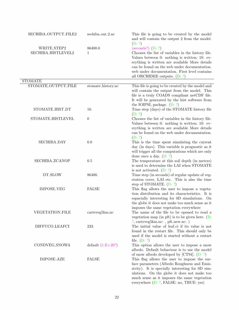
STOMATESTOMATE OUTPUT FILE stomate history.nc This file is going to be created by the model and
will contain the output from the model. Thisfile is a truly COADS compliant netCDF file.It will be generated by the hist software fromthe IOIPSL package. (D: ?)
STOMATE HIST DT 10. Time step (days) of the STOMATE history file(D: ?)
STOMATE HISTLEVEL 0 Chooses the list of variables in the history file.Values between 0: nothing is written; 10: ev-erything is written are available More detailscan be found on the web under documentation.(D: ?)
SECHIBA DAY 0.0 This is the time spent simulating the currentday (in days). This variable is prognostic as itwill trigger all the computations which are onlydone once a day. (D: ?)
SECHIBA ZCANOP 0.5 The temperature at this soil depth (in meters)is used to determine the LAI when STOMATEis not activated. (D: ?)
DT SLOW 86400. Time step (in seconds) of regular update of veg-etation cover, LAI etc. This is also the timestep of STOMATE. (D: ?)
IMPOSE VEG FALSE This flag allows the user to impose a vegeta-tion distribution and its characteristics. It isespacially interesting for 0D simulations. Onthe globe it does not make too much sense as itimposes the same vegetation everywhere
VEGETATION FILE carteveg5km.nc The name of the file to be opened to read avegetation map (in pft) is to be given here. (D:?, carteveg5km.nc: , pft new.nc: )
DIFFUCO LEAFCI 233. The initial value of leaf ci if its value is notfound in the restart file. This should only beused if the model is started without a restartfile. (D: ?)
CONDVEG SNOWA default (1.E+20?) This option allows the user to impose a snowalbedo. Default behaviour is to use the modelof snow albedo developed by [CT94]. (D: ?)
IMPOSE AZE FALSE This flag allows the user to impose the sur-face parameters (Albedo Roughness and Emis-sivity). It is specially interesting for 0D sim-ulations. On the globe it does not make toomuch sense as it imposes the same vegetationeverywhere (D: ?, FALSE: no, TRUE: yes)
22

SOILALB FILE soils param.nc The name of the file to be opened to readthe soil types from which we derive then thebare soil albedos. This file is 1x1 deg andbased on the soil colors defined by Wilson andHenderson-Seller. (D: ?)
SOILTYPE FILE soils param.nc (D: ?)ENERBIL TSURF 280. (K?) (D: ?)
hydrologyHYDROL SNOW 0.0 The initial value of snow mass if its value is not
found in the restart file. This should only beused if the model is started without a restartfile. (D: ?)
HYDROL SNOWAGE 0.0 The initial value of snow age if its value is notfound in the restart file. This should only beused if the model is started without a restartfile. (D: ?)
HYDROL SNOWICE 0.0 (D: ?)HYDROL SNOWICEAGE 0.0 (D: ?)
HYDROL HDRY 1.0 (D: ?)HYDROL HUMR 1.0 The initial value of soil moisture stress if its
value is not found in the restart file. Thisshould only be used if the model is started with-out a restart file. (D: ?)
HYDROL BQSB default (999999.?) The initial value (in kgm−2) of deep soil mois-ture if its value is not found in the restart file.This should only be used if the model is startedwithout a restart file. Default behaviour is asaturated soil. (D: ?)
HYDROL GQSB 0.0 The initial value (in kgm−2) of upper soil mois-ture if its value is not found in the restart file.This should only be used if the model is startedwithout a restart file. (D: ?)
HYDROL DSG 0.0 The initial value (in meters) of upper reservoirdepth if its value is not found in the restart file.This should only be used if the model is startedwithout a restart file. (D: ?)
HYDROL DSP default (999999.?) The initial value (in meters) of dry soil aboveupper reservoir if its value is not found in therestart file. This should only be used if themodel is started without a restart file. The de-fault behaviour is to compute it from the vari-ables above. Should be OK most of the time(D: ?)
HYDROL QSV 0.0 The initial value (in kgm−2) of moisture oncanopy if its value is not found in the restartfile. This should only be used if the model isstarted without a restart file.(D: ?)
HYDROL OK HDIFF n If TRUE, then water can diffuse horizontallybetween the PFTs’ water reservoirs. (D: ?, n:no, y: yes)
HYDROL TAU HDIFF 1800. Defines (in seconds) how fast diffusion occurshorizontally between the individual PFTs’ wa-ter reservoirs. If infinite, no diffusion. (D: ?)
THERMOSOIL TPRO 280. (K?) (D: ?)
23
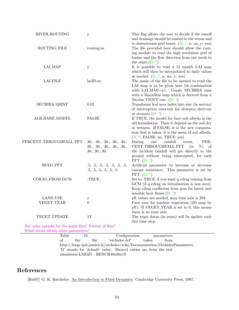
RIVER ROUTING y This flag allows the user to decide if the runoffand drainage should be routed to the ocean andto downstream grid boxes. (D: ?, n: no, y: yes)
ROUTING FILE routing.nc The file provided here should allow the rout-ing module to read the high resolution grid ofbasins and the flow direction from one mesh tothe other.(D: ?)
LAI MAP y It is possible to read a 12 month LAI mapwhich will then be interpolated to daily valuesas needed. (D: ?, n: no, y: yes)
LAI FILE lai2D.nc The name of the file to be opened to read theLAI map is to be given here (in combinationwith LAI MAP=n). Usualy SECHIBA runswith a 5kmx5km map which is derived from aNicolas VIOVY one. (D: ?)
SECHIBA QSINT 0.02 Transforms leaf area index into size (in meters)of interception reservoir for slowproc derivvaror stomate (D: ?)
ALB BARE MODEL FALSE If TRUE, the model for bare soil albedo is theold formulation. Then it depend on the soil dryor wetness. If FALSE, it is the new computa-tion that is taken, it is the mean of soil albedo.(D: ?, FALSE: no, TRUE: yes)
PERCENT THROUGHFALL PFT 30., 30., 30., 30., 30.,30., 30., 30., 30., 30.,30., 30., 30.
During one rainfall event, PER-CENT THROUGHFALL PFT (in %) ofthe incident rainfall will get directly to theground without being intercepted, for eachPFT. (D: ?)
RVEG PFT .5, .5, .5, .5, .5, .5, .5,.5, .5, .5, .5, .5, .5
Artificial parameter to increase or decreasecanopy resistance. This parameter is set byPFT. (D: ?)
CDRAG FROM GCM .TRUE. Set to .TRUE. if you want q cdrag coming fromGCM (if q cdrag on initialization is non zero).Keep cdrag coefficient from gcm for latent andsensible heat fluxes.(D: ?)
LAND USE y pft values are needed, max time axis is 293VEGET YEAR 0 First year for landuse vegetation (2D map by
pft). If VEGET YEAR is set to 0, this meansthere is no time axis.
VEGET UPDATE 1Y The veget datas (in years) will be update eachthis time step
Are other options for the input files? Format of files?What about all the other parameters?
Table 10: Configuration parametersof the file ’orchidee.def’ taken fromhttp://forge.ipsl.jussieu.fr/orchidee/wiki/Documentation/OrchideeParameters.’D’ stands for ’default’ value. Showed values are from the testsimulation LMDZ5 - BENCH48x36x19
References
[Bat67] G. K. Batchelor. An Introduction to Fluid Dynamics. Cambridge University Press, 1967.
24

[BE01] S. Bony and K. A. Emanuel. A parameterization of the cloudiness associated with cumulus convection;evaluation using toga coare data. J. Atmos. Sci., 58:3158–3183, 2001.
[BL95] O. Boucher and U. Lohmann. The sulfate-ccn-cloud albedo effect. Tellus B, 47(3):281–300, 1995.
[Cho77] E. Choisnel. Un modele agrometeorologique operationnel de bilan hydrique utilisant des donnees cli-matiques. Les besoins en eau des cultures. Proc. Conference internationale CIID. Paris, 1977.
[CT94] S. Chalita and H. Treut. The albedo of temperate and boreal forest and the northern hemisphereclimate: a sensitivity experiment using the lmd gcm. Climate Dynamics, 10(4-5):231–240, 1994.
[Dea66] J. W. Deardorff. The counter-gradient heat flux in the lower atmosphere and in the laboratory. J.Atmos. Sci., 23:503–506, 1966.
[DFD+13] J. L. Dufresne, M. A. Foujols, S. Denvil, A. Caubel, O. Marti, O. Aumont, Y. Balkanski, S. Bekki,H. Bellenger, R. Benshila, S. Bony, L. Bopp, P. Braconnot, P. Brockmann, P. Cadule, F. Cheruy,F. Codron, A. Cozic, D. Cugnet, N. Noblet, J. P. Duvel, C. Ethe, L. Fairhead, T. Fichefet, S. Flavoni,P. Friedlingstein, J. Y. Grandpeix, L. Guez, E. Guilyardi, D. Hauglustaine, F. Hourdin, A. Idelkadi,J. Ghattas, S. Joussaume, M. Kageyama, G. Krinner, S. Labetoulle, A. Lahellec, M. P. Lefebvre,F. Lefevre, C. Levy, Z. X. Li, J. Lloyd, F. Lott, G. Madec, M. Mancip, M. Marchand, S. Masson,Y. Meurdesoif, J. Mignot, I. Musat, S. Parouty, J. Polcher, C. Rio, M. Schulz, D. Swingedouw, S. Szopa,C. Talandier, P. Terray, N. Viovy, and N. Vuichard. Climate change projections using the ipsl-cm5 earthsystem model: from cmip3 to cmip5. Clim. Dyn., 40(9-10):2123–2165, 2013.
[DLP93] N. I. Ducoudre, K. Laval, and A. Perrier. Sechiba, a new set of parameterizations of the hydrologicexchanges at the land-atmosphere interface within the lmd atmospheric general circulation model. J.Climate, 6:248–273, 1993.
[dRP98] P. de Rosnay and J. J. Polcher. Modelling root water uptake in a complex land surface scheme coupledto a gcm. Hydrol. Earth Syst. Sci., 2(2/3):239–255, 1998.
[Ema91] K. A. Emanuel. A scheme for representing cumulus convection in large-scale models. J. Atmos. Sci.,48:2313–2329, 1991.
[Ema93] K. A. Emanuel. A cumulus representation based on the episodic mixing model: the importance ofmixing and microphysics in predicting humidity. AMS Meteorol. Monogr., 24:185–192, 1993.
[EuR99] K. A. Emanuel and M. Zivkovic Rothman. Development and evaluation of a convection scheme for usein climate models. J. Atmos. Sci., 56:1766–1782, 1999.
[FB80] Y. Fouquart and B. Bonnel. Computations of solar heating of the earth’s atmosphere: A new parame-terization. Beitr. Phys. Atmos., 53:35–62, 1980.
[Fou88] Y. Fouquart. Radiative transfer in climate models. In M.E. Schlesinger, editor, Physically-BasedModelling and Simulation of Climate and Climatic Change, volume 243 of NATO ASI Series, pages223–283. Springer Netherlands, 1988.
[Gel77] J. F. Geleyn. A comprehensive radiation scheme designed for fast computation. Res. Dep. Eur. Cent.for Medium Range Weather Forecasts, Reading, England, Internal Rep. 8.:36, 1977.
[GL09] J. Y. Grandpeix and J. P. Lafore. A density current parameterization coupled with emanuels convectionscheme. part i: The models. J. Atmos. Sci., 67:881–897, 2009.
[GLC09] J. Y. Grandpeix, J. P. Lafore, and F. Cheruy. A density current parameterization coupled with emanuelsconvection scheme. part ii: 1d simulations. J. Atmos. Sci., 67:898–922, 2009.
[GPT04] J. Y. Grandpeix, V. Phillips, and R. Tailleux. Improved mixing representation in emanuel’s convectionscheme. Q. J. R. Meteorol. Soc., 130(604):3207–3222, 2004.
[Gur65] M. I. Gurevich. Theory Of Jets In Ideal Fluids. Academic Press (Translated From The Russian Edition),1965.
25

[HCM02] F. Hourdin, F. Couvreux, and L. Menut. Parameterization of the dry convective boundary layer basedon a mass flux representation of thermals. J. Atmos. Sci., 59:1105–1123, 2002.
[HD90] A. J. Heymsfield and L. J. Donner. A scheme for parameterizing ice-cloud water content in generalcirculation models. J. Atmos. Sci., 47:1865–1877, 1990.
[HFC+13] F. Hourdin, M. A. Foujols, F. Codron, V. Guemas, J. L. Dufresne, S. Bony, S. Denvil, L. Guez, F. Lott,J. Ghattas, P. Braconnot, O. Marti, Y. Meurdesoif, and L. Bopp. Impact of the lmdz atmosphericgrid configuration on the climate and sensitivity of the ipsl-cm5a coupled model. Climate Dynamics,40(9-10):2167–2192, 2013.
[HGR+13] F. Hourdin, J. Y. Grandpeix, C. Rio, S. Bony, A. Jam, F. Cheruy, N. Rochetin, L. Fairhead, A. Idelkadi,I. Musat, J. L. Dufresne, A. Lahellec, M. P. Lefebvre, and R. Roehrig. Lmdz5b: the atmosphericcomponent of the ipsl climate model with revisited parameterizations for clouds and convection. Clim.Dyn., 40(9-10):2193–2222, 2013.
[Jar76] P. G. Jarvis. The interpretation of the variations in leaf water potential and stomatal conductancefound in canopies in the field. Phil. Trans. R. Soc. Lond. B, 273:593–610, 1976.
[JHRC11] A. Jam, F. Hourdin, C. Rio, and F. Couvreux. Resolved versus parameterized boundary-layer plumes.part iii: a diagnostic boundary-layer cloud parameterization derived from large eddy simulations.submitted to BLM, 2011.
[Kir77] G. Kirchoff. Vorlesungen uber mathematische physik. Mechanik / von Dr.Gustav Robert Kirchhoff.Leipzig, 1877.
[KVdND+05] G. Krinner, N. Viovy, N. de Noblet-Ducoudre, J. Ogee, J. Polcher, P. Friedlingstein, P. Ciais, S. Sitch,and I. C. Prentice. A dynamic global vegetation model for studies of the coupled atmosphere-biospheresystem. Global Biogeochem. Cy., 19(1):n/a–n/a, 2005.
[Lan61] L. Landweber. Motion of immersed and floating bodies. McGraw-Hill (1st ed.), 1961.
[LLLF80] T. Lohammar, S. Larsson, S. Linder, and S. O. Falk. Fast: Simulation models of gaseous exchange inscots pine. Ecological Bulletins, 32:505–523, 1980.
[LM97] F. Lott and M. J. Miller. A new subgrid-scale orographic drag parametrization: Its formulation andtesting. Q. J. R. Meteorolo. Soc., 123(537):101–127, 1997.
[Mat83a] E. Matthews. Global vegetation and land use: New high-resolution data bases for climate studies. J.Climate Appl. Meteor., 22:474–487, 1983.
[Mat83b] E. Matthews. Prescription of land-surface boundary conditions in giss gcm ii: A simple method basedon high-resolution vegetation data bases. Tech. Memo. NASA, 86096:20, 1983.
[Mat84] E. Matthews. Vegetation, land-use and seasonal albedo data sets: documentation of archived data tape.Tech. Memo. NASA, 86107:12, 1984.
[MF85] J. J. Morcrette and Y. Fouquart. On systematic errors in parametrized calculations of longwave radiationtransfer. Q. J. of R. Meteorol. Soc., 111(469):691–708, 1985.
[MF86] J.J. Morcrette and Y. Fouquart. The overlapping of cloud layers in shortwave radiation parameteriza-tions. J. Atmos. Sci., 43:321–328, 1986.
[MFS+72] R. A. McClatchey, R. W. Fenn, J. E. A. Selby, F. E. Volz, and J. S. Garing. Optical Properties ofthe Atmosphere. Environ. Res. Pap. (3rd Ed.) Air Force Cambridge Research Labs Hanscom Afb MA,1972.
[Mon63] J. L. Monteith. Gas exchange in plant communities. Academic Press, New York, USA, 1963.
[Mor90] J.J. Morcrette. Impact of changes to the radiation transfer parameterizations plus cloud optical. prop-erties in the ecmwf model. Mon. Wea. Rev., 118:847–873, 1990.
26

[Mor91] J. J. Morcrette. Radiation and cloud radiative properties in the european centre for medium rangeweather forecasts forecasting system. J. Geophys. Research: Atmospheres, 96(D5):9121–9132, 1991.
[MSF86] J. J. Morcrette, L. Smith, and Y. Fouquart. Pressure and temperature dependence of the absorption inlongwave radiation parametrizations. Beitrage zur Physik der Atmosphare, 59:455–469, 1986.
[MY74] G. L. Mellor and T. Yamada. A hierarchy of turbulence closure models for planetary boundary layers.J. Atmos. Sci., 31:1791–1806, 1974.
[Phi84] D. S. Phillips. Analytical surface pressure and drag for linear hydrostatic flow over three-dimensionalelliptical mountains. J. Atmos. Sci., 41:1073–1084, 1984.
[RH08] C. Rio and F. Hourdin. A thermal plume model for the convective boundary layer: Representation ofcumulus clouds. J. Atmos. Sci., 65:407–425, 2008.
[RHCJ10] C. Rio, F. Hourdin, F. Couvreux, and A. Jam. Resolved versus parametrized boundary-layer plumes.part ii: Continuous formulations of mixing rates for mass-flux schemes. Boundary-Layer Meteorology,135(3):469–483, 2010.
[SC81] N. A. Scott and A. Chedin. A fast line-by-line method for atmospheric absorption computations - theautomatized atmospheric absorption atlas. J. of Appl. Meteor., 20:802–812, 1981.
[Shu88] W. J. Shuttleworth. Evaporation from amazonian rainforest. Proc. R. Soc. Lond. B, 233:321–346, 1988.
[SK91] B. Saugier and N. Katerji. Some plant factors controlling evapotranspiration. Agric. Forest Meteor.,54(2-4):263 – 277, 1991.
[SSP+03] S. Sitch, B. Smith, I. C. Prentice, A. Arneth, A. Bondeau, W. Cramer, J. O. Kaplan, S. Levis, W. Lucht,M. T. Sykes, K. Thonicke, and S. Venevsky. Evaluation of ecosystem dynamics, plant geography andterrestrial carbon cycling in the lpj dynamic global vegetation model. Global Change Biol., 9(2):161–185,2003.
[SSR+89] N. Sato, P. J. Sellers, D. A. Randall, E. K. Schneider, J. Shukla, J. L. Kinter, Y. T. Hou, and E. Al-bertazzi. Effects of implementing the simple biosphere model in a general circulation model. J. Atmos.Sci., 46:2757–2782, 1989.
[Ste78] G. L. Stephens. Radiation profiles in extended water clouds. ii: Parameterization schemes. J. Atmos.Sci., 35:2123–2132, 1978.
[Stu88] R. B. Stull. An introduction to boundary layer meteorology. Kluwer Academic Publishers, 1988.
[Sun78] H. Sundqvist. A parameterization scheme for non-convective condensation including prediction of cloudwater content. Q. J. R. Meteorol. Soc., 104(441):677–690, 1978.
[Sun88] H. Sundqvist. Parameterization of condensation and associated clouds in models for weather predic-tion and general circulation simulation. In M.E. Schlesinger, editor, Physically-Based Modelling andSimulation of Climate and Climatic Change, volume 243 of NATO ASI Series, pages 433–461. SpringerNetherlands, 1988.
[Vig53] E. Vigroux. Contribution a l’etude experimentale de l’absorption de l’ozone. Ann. Phys., 8:709, 1953.
[WMO84] WMO. The intercomparison of radiation codes in climate models (icrccm), longwave, clear-sky calcu-lations. World Climate Programme, Geneva, Switzerland, Rep. WCP-93:37, 1984.
[Yam83] T. Yamada. Simulations of nocturnal drainage flows by a q2l turbulence closure model. J. Atmos. Sci.,40:91–106, 1983.
[ZK97] C. S. Zender and J. T. Kiehl. Sensitivity of climate simulations to radiative effects of tropical anvilstructure. J. Geophys. Res.: Atmospheres, 102(D20):23793–23803, 1997.
27