See discussions, stats, and author profiles for this publication at: https://www.researchgate.net/publication/40222532

Living in a Battleground: Presidential Campaigns and Fundamental Predictors of

Vote Choice

Article  in  Political Research Quarterly · September 2009

DOI: 10.1177/1065912908319575 · Source: OAI

CITATIONS

20READS

79

2 authors:

Some of the authors of this publication are also working on these related projects:

Mayoral elections View project

Scott Mcclurg

Southern Illinois University Carbondale

62 PUBLICATIONS   2,112 CITATIONS   

SEE PROFILE

Thomas M. Holbrook

University of Wisconsin - Milwaukee

62 PUBLICATIONS   2,361 CITATIONS   

SEE PROFILE

All content following this page was uploaded by Scott Mcclurg on 30 December 2013.

The user has requested enhancement of the downloaded file.

Southern Illinois University CarbondaleOpenSIUC

Publications Department of Political Science

1-1-2009

Living in a Battleground: Presidential Campaignsand Fundamental Predictors of Vote ChoiceScott D. McClurgSouthern Illinois University, mcclurg@siu.edu

Thomas M. HolbrookUniversity of Wisconsin - Milwaukee, holbroot@uwm.edu

Follow this and additional works at: http://opensiuc.lib.siu.edu/ps_pubs

This Article is brought to you for free and open access by the Department of Political Science at OpenSIUC. It has been accepted for inclusion inPublications by an authorized administrator of OpenSIUC. For more information, please contact jnabe@lib.siu.edu.

Recommended CitationMcClurg, Scott D. and Holbrook, Thomas M., "Living in a Battleground: Presidential Campaigns and Fundamental Predictors of VoteChoice" (2009). Publications. Paper 5.http://opensiuc.lib.siu.edu/ps_pubs/5

Living in a Battleground: Presidential Campaigns

and Fundamental Predictors of Vote Choice

Scott D. McClurg, Associate Professor Department of Political Science

Southern Illinois University 3165 Faner Hall Mailcode 4501

Carbondale, IL 62901-4501 mcclurg@siu.edu

Thomas M. Holbrook, Professor Department of Political Science

University of Wisconsin, Milwaukee PO Box 413

3210 N. Maryland Avenue Milwaukee, WI 53201

holbroot@uwm.edu

Published in

Political Research Quarterly, 2009, 62(3):495-06. Paper prepared for presentation at the 2005 Annual Meeting of the Midwest Political Science Association, Chicago, IL, April 2nd – 5th, 2005. This is a pre-typeset version of a peer-reviewed paper published in Political Research

Quarterly developed for deposit on the SIUC institutional repository. All references should refer to the published version, details given above.

Holbrook and McClurg, “Mechanisms, p. 2

Abstract

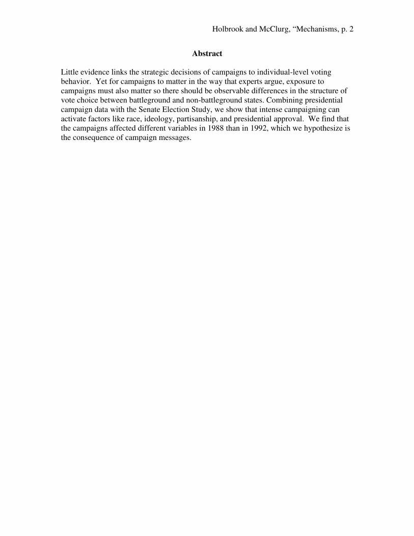
Little evidence links the strategic decisions of campaigns to individual-level voting behavior. Yet for campaigns to matter in the way that experts argue, exposure to campaigns must also matter so there should be observable differences in the structure of vote choice between battleground and non-battleground states. Combining presidential campaign data with the Senate Election Study, we show that intense campaigning can activate factors like race, ideology, partisanship, and presidential approval. We find that the campaigns affected different variables in 1988 than in 1992, which we hypothesize is the consequence of campaign messages.

Holbrook and McClurg, “Mechanisms, p. 1

Introduction

An emerging scholarly consensus that campaigns matter in elections is built on

evidence showing that the public reacts to campaign events (Holbrook 1996; Hillygus

2005), the issue context of elections influences vote choice (Clinton and Lapinski 2004;

Carsey 2000; Simon 2002; Popkin 1991), and aggregate election results are related to

campaign intensity (Shaw 1999a; Holbrook and McClurg 2005). While such work

refutes long-held notions that campaigns have “minimal effects,” limits remain to our

evidence on whether voting behavior would be different in the absence of presidential

campaigns. In this paper we address this by examining whether the intense flows of

information created by presidential campaigns in some locales but not elsewhere produce

differences in voting behavior.

Unlike most previous research, we examine how campaign decisions create

geographically-driven information contexts in order to explicitly link them to voter

decision-making. In particular, we examine how fundamental predictors of vote choice

like partisanship and presidential evaluation vary in importance across campaign contexts

of different intensity. By combining survey data from the Senate Election Study with a

unique measure of state-wide campaign intensity from the 1988 and 1992 presidential

elections, our study makes two contributions to knowledge on presidential campaign

effects. First, we show that individual voting can differ dramatically across campaign

context thus providing rare individual-level evidence of campaign effects that result from

the strategic allocation of campaign resources over the electoral map. Second, our results

suggest a dependence of such effects between years on the choice of campaign message.

Though this second hypothesis bears further testing in future research, the fact that the

Holbrook and McClurg, “Mechanisms, p. 2

variables which are more important in battleground states than non-battleground states

varies across election years is highly suggestive of this point.

Research on Campaign Effects

For years, campaign effects research was plagued by a contradiction between

common sense beliefs that campaigns influence voters and generally mild empirical

evidence of such effects. Two arguments emerged as political scientist’s reconciled

instinct with evidence. The first is that campaigns are strategic, with opposing candidates

concentrating resources on the same locations (Shaw 1999b, 2006) and targeting subsets

of the voting population (Huber and Arceneaux in press; Gerber and Green 2004, Chapter

1; Goldstein and Ridout 2002; Abramson and Claggett 2001; Huckfeldt and Sprague

1992). From this perspective, strategic considerations and selection processes mask

campaign effects. That is, the competitive pressures faced by campaigns minimize their

aggregate and individual effects. Seeking to avoid this problem, scholars use

experimental designs to investigate the impact of negative advertising (Ansolabehere and

Iyengar 1995), information complexity (Barker and Hansen 2005; Lau and Redlawsk

2001), issue engagement (Simon 2002), and contacting techniques (Gerber and Green

2004; Green and Gerber 2005) on voting behavior. Still others use quasi-experimental

designs to gain significant leverage using data from real campaigns (Huber and

Arceneaux, in press) by focusing on voters in targeted media markets who are not in

targeted states. The general consensus of these studies is that campaigns can influence

voters.

A second perspective sees campaigns as a series of events that are related in time,

with the people who run them making decisions on a day-to-day basis, often in reaction

Holbrook and McClurg, “Mechanisms, p. 3

to events outside of their control. When such dynamics are ignored, the argument goes,

changes in public behavior that occur during the election are overlooked. Accordingly,

studies based on cross-sectional designs use an operational concept of campaigns that

does not match reality and therefore find weak effects. Gelman and King (1994),

Holbrook (1996), Wlezien and Erickson (2002), Hillygus and Jackman (2003), and

Johnston, Hagen, and Jamieson (2005) all use longitudinal evidence from within a single

campaign cycle to illustrate the impact of specific campaign events on the electorate,

while Shaw (1999a, 2006) specifically demonstrates the effect of ad buys and campaign

visits on statewide and media market outcomes.

Though such research puts to rest lingering doubts about whether campaigns

influence elections, there are still limits to what we know. For example, experimental

studies convincingly establish that voters can be influenced by advertising content and

polarity but ultimately do not show that they do influence them in the complex

environments characterizing actual campaigns where strategy might minimize actual

effects. Likewise, scholars interested in dynamic effects understandably focus on

specific events (e.g., debates, conventions) or the impact of the campaign in its entirety

(i.e., not measuring variation in campaign behavior), rather than the behavioral

heterogeneity produced by campaign decisions that are reflected in geographic disparities

in campaigning. What remains to be seen in this literature is whether real campaigns

influence individual behavior in meaningful ways through their strategic decisions. 1 In

this paper we address these issues by, first, focusing on differences in real campaign

context and, second, by examining how the underlying considerations of vote choice then

differ in impact across campaign context. To our knowledge, there is no other study that

Holbrook and McClurg, “Mechanisms, p. 4

examines the relationship between presidential campaign context and the impact of

traditional predictors on vote choice. 2

Campaign Effects and Predictors of Vote Choice

This paper tests the proposition that, given the inequitable distribution of

campaign resources across the fifty states, where voters live determines the amount and

type of campaign information available to them, and this in turn has important

consequences for how the vote is structured. Consider two states whose names are easily

confused but whose campaign experiences in the 2004 election could not be more

different, Iowa and Idaho. Neither presidential candidate visited Idaho, nor were there

any media buys there by the candidates or parties in 2004. At the same time Iowa was

subjected to 17 campaign appearances by the presidential candidates, another 24

appearances by the vice-presidential candidates, and enough media buys that the average

Iowan could have seen 310 campaign ad airings.3 These are starkly different information

environments and we expect that these differences have significant consequences for the

structure of voter decisions.

We expect that voters living in states with intense exposure to the campaign differ from

voters living in states with relatively little direct exposure in two important ways. First,

we expect that their vote will be more structured and easily predicted by fundamental

considerations. Second, we expect that the mix of considerations voters bring to bear on

the vote will differ across campaign contexts. These effects, we argue, stem from how

voter predispositions are connected to candidates during campaigns. Here, our work is

informed by a stream of research that begins with Berelson et al.’s (1954) emphasis on

activation. They note that most voter change during campaigns comes from partisans

Holbrook and McClurg, “Mechanisms, p. 5

who “return to the fold” (also see Finkel 1993). More broadly, Gelman and King (1993)

show that pre-election trial-heat polls became better predictors of the actual election

outcomes as the election draws near, suggesting that campaigns “enlighten voters.”

Several studies have taken up Gelman and King’s hypothesis with generally encouraging

results (Stevenson and Vavreck 2000; Arceneaux 2005; Holbrook and McClurg 2005;

Hillygus and Jackman 2003). While these earlier demonstrations presumed that

campaign information makes it easier for voters to cast their ballots the way one might

expect them to given their underlying predispositions, there is no direct demonstration

that such effects derive from exposure to specific information environments created by

the campaigns or the extent to which it operates through voter predispositions.

We assume that campaigns choose campaign messages based on the composition

of the electorate as well as the prevailing issues and conditions of the day in order to tap

voter attributes that have a prior history of affecting the vote and then allocate resources

to communicate that message in the most efficient manner possible (Shaw 2006). The

idea here is that campaigns build their influence in elections by appealing to voter

predispositions. We are agnostic about the specific psychological mechanisms

underlying these connections; they might occur through agenda setting, persuasion, or

priming. The key point is that campaign messages are used to help increase the

connection between pre-existing voter attributes and interests and a specific candidate. It

is not merely a consequence of having an election, per se, so much as being exposed to

campaign information that strengthens the connection between voter predilections and the

choice between candidates.

Holbrook and McClurg, “Mechanisms, p. 6

While prior research conceives of this process almost solely in terms of

partisanship (e.g., Finkel 1993; Berelson et al. 1954; but see Kahn and Kenny 1999),

there is no reason to expect campaign to focus only on partisanship. Though it remains

an important way of connecting with voters, candidates would be remiss if they tried to

tap partisanship at the expense of appealing to voters who are happy about a booming

economy or upset with a flagging presidency. We therefore expect that a broad array of

fundamental considerations, including party identification, presidential approval,

ideology, economic evaluations, etc., can be the raw material that campaigns tap through

their resource allocation and communication strategies.

Most critically, our approach differs in that we conceive of campaigns as being as

much a function of space as of time (in contrast, see Bartels 2006). As Shaw (2006)

demonstrates, the imperative to expend resources in as efficient a manner possible leads

campaigns to create dramatically different campaign contexts across both states and

media markets. If campaign effects depend on what campaigns communicate to voters,

those voters who are most directly exposed to that information should be more strongly

influenced by it than those who are relatively unexposed. Specifically, voters in

battleground states – where campaign information is plentiful – will behave differently

than fellow citizens in states that are ignored by the campaigns and therefore relatively

information poor with respect to the specific messages constructed by the presidential

campaigns. In short voting behavior is jointly produced by a combination of

predispositions and campaign context, rather than each type of factor separately.

What of voters in non-battleground states? Does our framework imply that they

are choosing at random? Are they basing their votes on something other than

Holbrook and McClurg, “Mechanisms, p. 7

information? In a word, no. We do not claim that voters in these states are uninformed

or that their behavior is un-structured. Indeed, we fully expect that voters in the rest of

the county are exposed to campaign messages through media coverage of campaign

events, including those in the battleground states.

But in a very real sense, they are experiencing the presidential campaign much

differently than voters in battleground states. First, they have less exposure to the

specific messages, debates, and symbols that the campaigns use to influence voting

behavior. Second, to the extent that they do receive campaign information, it is heavily

mediated. As the media are more likely to present multiple points of view, provide

alternative interpretations of issues and messages, and to focus on campaign strategy or

horse race coverage, there is more ambiguity in what the information implies for voters.

Altogether this means that intense campaign environments create more opportunities for

underlying campaign messages to get to voters and in such a way that the intended

meanings are less ambiguous for voters.

As a consequence, if campaigns do in fact affect voting behavior by activating

voter fundamentals with campaign information, we should find that voters in

battleground states choose differently than voters in other states. If this is not the case

and we do not observe differences between voters in battleground and non-battleground

states, it importantly implies that campaign decisions about what to communicate, where

to communicate it, and when are unimportant for how they influence voter decision-

making. This in turn would imply a different model of “campaign effects” that

downplays the role of resource allocation and highlights other considerations.

Data and Methods

Holbrook and McClurg, “Mechanisms, p. 8

Measuring the Battleground States. Testing our argument hinges on the fact that

presidential campaigns do not distribute resources equitably across states (Shaw 1999a,

2006). Since states are unequal in terms of advertising costs, competitiveness, and

Electoral College votes, presidential campaigns choose to spend almost no resources in

some states while saturating others with visits, commercials, campaign paraphernalia,

voter contacts, and the like. The end result is that not all voters live in the same

campaign context, providing us with the opportunity to study campaigns by treating them

as contextual effects. Since our hypotheses focus on differences in voting behavior that

are a product of campaign contexts, we need a valid measure of state campaign intensity.

We use three readily available indicators of presidential campaign behavior to

build our measure. Two of them – presidential advertising purchases and candidate visits

– were gathered by Daron Shaw and made available in his 1999 American Political

Science Review article. The third is a measure of national party monetary transfers to the

states.4 Including party transfers is important because they played an important role in

presidential campaigns throughout the 1990s and because they are more widely

distributed across states, thus providing additional variation in our key independent

variable. We combine these three indicators by standardizing each within campaign year

and then summing them together into a single measure of campaign intensity. This then

is used as the basis for identifying the battleground states: those states in the top third of

the summary measure in each of the election years.5

Since our survey data are for 1988 and 1992 (see below), we can establish validity

for our measure by comparing it to Shaw’s (1999b) data on Electoral College strategies

that are gleaned from the campaign's strategy memos. Of all the states he identifies as

Holbrook and McClurg, “Mechanisms, p. 9

being considered a “battleground” by both campaigns, all of them are similarly measured

with our data. Moreover, of all the states identified as a battleground by at least one of

the campaigns, we are consistent in all but two cases (out of seventeen). Although we

pick up a fair amount of campaigning in states that are not listed in Shaw’s classification

(e.g., South Carolina in 1988), the vast majority of those are cases in which the data show

the campaign did not follow their plan and therefore did campaign in those states. All in

all, we believe this clearly establishes the validity of our battleground measure.6

Individual-Level Data. Investigating our hypotheses also requires individual-

level observational data within the states. Two criteria exist for the individual-level data:

1) there must be a large enough sample size within each state to produce stable

coefficient estimates and 2) our respondents must have been surveyed at approximately

the same time to minimize the impact of temporal dynamics as an alternative explanation.

Although there are many national survey samples with appropriate sample sizes or the

appropriate measures, only the Senate Election Study (Miller et al. 1999) meets both

these criteria. This study was constructed primarily for studying views of Senators and

senatorial candidates in each electoral year from 1988 to 1992. However, it includes

many of the variables essential for studying presidential voting behavior and is therefore

useful for our purposes.

In 1988 and1992, roughly 60 voting-age citizens were interviewed in each of the

50 states.7 For this study, we draw on the 1988 and 1992 data which provides us with

approximately 5,859 survey responses. Of this sample, 4,394 reported voting in the

November elections (4,344 in the presidential election) with 3,857 respondents providing

a presidential vote choice. From this study we draw the basic independent variables for

Holbrook and McClurg, “Mechanisms, p. 10

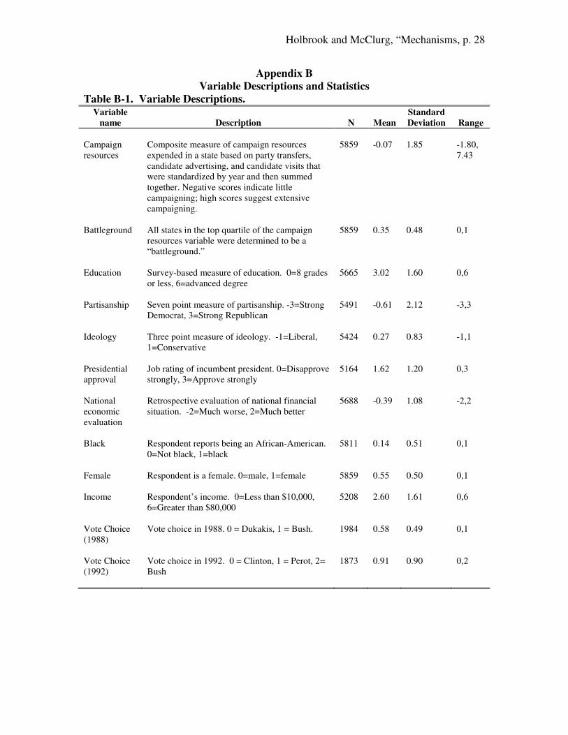
the analysis, each of which is described and summarized in Appendix B. They include

familiar predictors of vote choice available in the National Election Study, such as

partisanship, race, ideology, etc. To account for the unique structure of these data, all of

our estimates use appropriate population weights and clustered standard errors by state.

Vote Choice, Fundamental Considerations, and Campaign Context

We now turn to an examination of how campaign intensity influences the mix of

variables that are important to presidential vote choice. It is important at the outset to be

clear that our interest here is not just in whether there is a direct relationship between

campaign activity and vote choice, but rather in how the campaigns structure the

underlying determinants of vote choice and make them better (or stronger) predictors of

what citizens do. Our logic here flows directly from the proposition that campaigns

engage “fundamental” considerations such as partisanship and presidential evaluations

(Campbell 2000; Gelman and King 1993). The basic idea is that campaigns deliver

messages that reinforce party identification and remind voters of the issues at hand,

especially those related to presidential performance. If this is the case, then we expect to

see the fundamentals of vote choice play a stronger role in states in which the presidential

campaign is intense than in states in which the level of campaign activity is relatively

minimal.8 We also develop and test a fundamental vote choice model and examine its

results under different campaign contexts. The model includes measures of partisanship,

presidential approval, economic attitudes, political ideology, and demographic

characteristics.9

The analysis of the differential impact of fundamental considerations in

battleground and non-battleground states is presented in Tables 1 and 2. In both of these

Holbrook and McClurg, “Mechanisms, p. 11

tables we regress vote choice on the basic model for the full sample and then also for the

battleground and non-battleground samples. There are two general questions that we

answer here. First, does the model of fundamental considerations “fit” better in

battleground states than in other states and, second, are certain fundamental

considerations activated by the campaign to produce significantly stronger effects in the

battleground states than in other states?

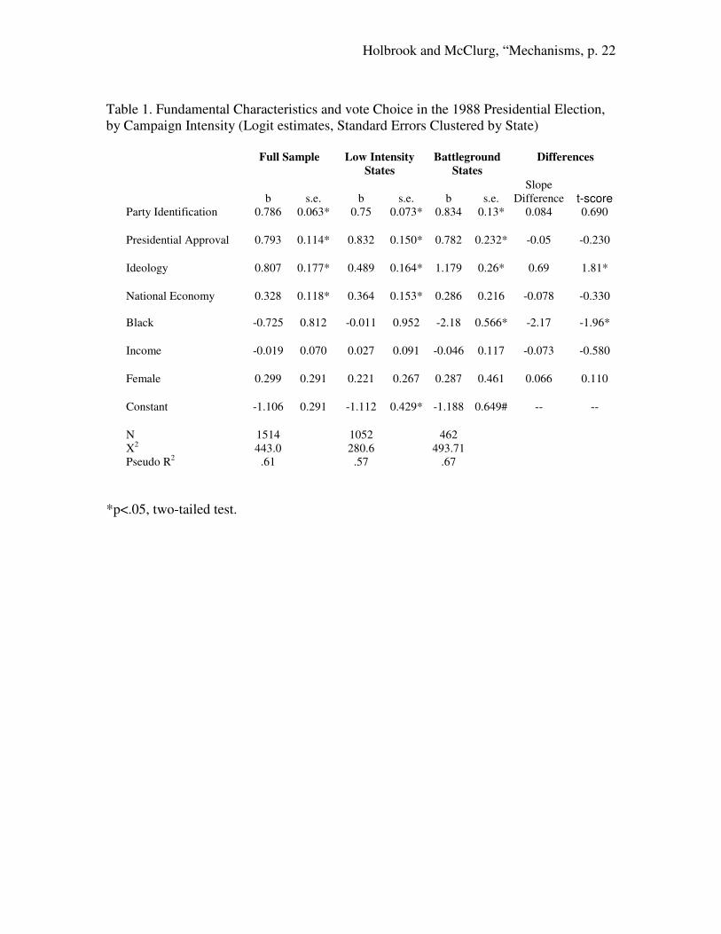
Turn to the analysis of the 1988 election presented in Table 1, where the choice

between Bush and Dukakis is estimated with a logit model. Here we see that the

fundamental model is strongly related to vote choice and that the variables we expect to

be important (party, approval, ideology economy) obtain standard levels of statistical

significance. Turning to the issue of whether the model overall performs better in the

battleground states, we see that the pseudo R2 is .57 in low intensity states and .67 in

battleground states. On its face, this looks like a significant increase in explanatory

power. When put to a test of statistical significant, however, we find the difference is

marginally significant (p=.076).10

[Table 1 about here]

With respect to specific coefficients we see that while many of the differences are

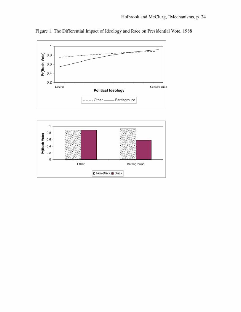
trivial, two variables – ideology and race – stand out as significantly stronger in the

battleground states than in other states.11 We can gain an appreciation of the magnitude of

these differences by turning to Figure 1, which plots the probability of casting a vote for

Bush for different levels of ideology and race (all other variables set to their median

values). Here we see a relatively flat slope for ideology in non-battleground states and a

much steeper slope in battleground states. The total estimated difference in probability of

Holbrook and McClurg, “Mechanisms, p. 12

voting for Bush between a very liberal and very conservative respondent was .14 in non-

battleground states and fully .39 in battleground states. The lower part of Figure 1 shows

how race was activated by the 1988 campaign. Here we see that there was no racial gap

in voting in non-battleground states but a substantial gap in battleground states, where the

difference in the probability of voting for Bush between black respondents and all others

was .33.

[Figure 1 about here]

In Table 2 we find results that are similar in that the campaign seems closely

related to the impact of fundamentals in 1992, but different in that the specific

fundamentals affected are themselves not the same as in 1988.12 Here we see additional

evidence that different sets of considerations are important in battleground states than in

other states. Focusing again on the overall fit of the model we see that the pseudo R2 in

battleground states (.60) is substantially larger than in other states (.48), thus indicating

that, as a whole, the fundamental variables used in this model more adequately explain

vote choice where the campaign is intense than where it is not.13 To be sure, the vote is

still structured in non-battleground state, just not as structured by the fundamental

considerations as in battleground states.

[Table 2 about here]

An examination of the individual coefficients reveals some additional, mostly

intuitive, differences between the two models.14 First, the fundamental considerations of

party identification and presidential approval are much stronger determinants of vote

choice in battleground states than in other states. Not only is the difference in slopes

statistically significant but also it is substantively very important. The top two panes of

Holbrook and McClurg, “Mechanisms, p. 13

Figure 2 illustrate how the influence of party identification and presidential approval on

vote choice is conditioned campaign intensity. In both cases the translation of attitude

into vote is much swifter and stronger in battleground states than in other states. These

differences are exactly what might be expected given our hypothesis.

We do have one important contrary finding in Table 2 – economic evaluations are

significantly related to vote choice in low intensity states but not in battleground states.

One possibility is that given the dramatic influence of presidential approval in

battleground states, economic evaluation are subsumed under that broader evaluation. A

second possibility is that some complex relationship among partisanship, presidential

approval and economic evaluations is producing this unexpected result. There is some

evidence for both explanations. A bivariate analysis shows that the economic attitude-

vote relationship is stronger in battleground states (Cramer’s V=.35) than in the other

states (Cramer’s V=.28). Moreover, economic evaluations are more strongly determined

by partisanship and approval in battleground states (R2=.28) than in the other states

(R2=.18).15

Otherwise we are at a loss to explain this anomaly, except to say that the impact

of economic evaluations is really quite meager compared to the impact of party

identification and presidential approval. The bottom pane of Figure 2 makes this point

fairly clearly. Here we see that while that while economic evaluations are of some

consequence in non-battleground states (the slope for battleground states is not

significant), their impact pales in comparison to the other considerations in Figure 2 and,

overall, contribute much less to the overall explanation. Finally, the slope for respondent

sex is significant and in an unexpected direction in battleground states but not significant

Holbrook and McClurg, “Mechanisms, p. 14

in other states. While this is the case, the difference in slopes between the two samples is

not statistically significant.

Why Does the Impact of Campaign Fundamentals Differ From 1988 to 1992?

While we expected to find that campaigns would influence the relevance of

factors other than partisanship on voting, we did not expect to find that partisanship

would not be activated in the 1988 campaign or that factors impacted by the campaign

would matter significantly from 1988 to 1992. This raises an interesting question, though

one we had not anticipated – why are these fundamentals influenced rather than others?

We are able to spin a post hoc answer that is related to the themes of the campaign that

we believe has merit, though one that is admittedly is in need of additional empirical

testing.16

The foundation for this conjecture comes from Berelson et al.’s original

arguments about activation, particularly when we consider their interpretation of Harry

Truman’s comeback in the 1948 presidential election. According to them, Truman’s

recovery was not due to changes in evaluations of his character or competence but to an

increase in the salience of class-related issues late in the campaign:

The campaign was characterized by a resurgence of attention to socioeconomic maters, at the expense of international issues. The image of Truman did not change, but the image of what was important in the campaign--and perhaps even the image of what Truman stood for--did change to a dominance of socioeconomic issues (1954:264).

In effect they argue that, as Truman shifted the focus of the campaign to class issues, he

activated those considerations among his wandering supporters and they came home to

vote for him. We suspect that this same argument applies to our data as well, with the

type of issues raised by the campaigns influencing the type of fundamental considerations

Holbrook and McClurg, “Mechanisms, p. 15

that loom larger in people’s voting calculations across years. And, as campaign strategy

provides for more intense, less ambiguous information environments these ought to have

a larger impact on voters in battleground states than in non-battleground states.

At first blush, the cross-campaign differences are sensible. For example, the 1988

campaign was marked by racial overtones. Of particular interest here are the findings

from Mendelberg’s (2001) analysis, which showed that the Willie Horton ad (and

coverage of it) not only primed racial attitudes but also primed ideology as an influence

on candidate evaluations in the 1998 presidential contest. In addition, Gwiasda’s (2001)

finding that media coverage of the Willie Horton ad had an influence on general

perceptions of Michael Dukakis’ ideological position also buttresses our findings.

Similarly, Geer (2005, p. 91) shows that a key racial issue – crime – was intensely pushed

by George Bush in his negative advertising (27-percent of all Republican negative ads

that year).

In contrast, the 1992 is often remembered for emphasizing the poor performance

of the incumbent administration, particularly with regards to the economy. In that sense,

it is a classic retrospective-voting election with – importantly – blame focused on the tax

increases agreed to by the Bush administration and responsibility for the economic

downturn being laid at his feet by the Clinton campaign. Illustrative evidence comes

from Geer’s account of advertising in the 1992 campaign. The Clinton campaign ran

over 30-percent of their negative ads on “economic times,” while the Bush campaign ran

over 30-percent on taxes (with Clinton running 17-percent of his positive ads on taxes as

well, essentially claiming he would not increase taxes on any but the rich).

Holbrook and McClurg, “Mechanisms, p. 16

We would be remiss if we did not point out that accepting this as a possible

interpretation requires us to believe that the economic question was less about feelings on

the economy than it was a review of President Bush’s performance and that we have no

strong evidence supporting that assertion. Yet, it is not entirely inconsistent with other

evidence on voting behavior in 1992, as well as our own finding about how economic

factors behave as expected when incumbent evaluations are dropped from our model.

For example, Holbrook (1994) shows that consumer sentiment had an impact on

candidate preferences that was roughly 1/3rd as large as the impact as presidential

evaluation in a model that controls for the sequence of campaign events, but not for

geographical differences in campaigning. Similarly, Hetherington (1996) shows that the

standardized coefficient for candidate evaluation – an indirect measure of presidential

popularity – is roughly four times as large as it is for economic evaluations in influencing

vote choice. While none of this is definitive proof of our assumption, it is generally

consistent with the hypothesis.

However, we believe that this hypothesis warrants closer attention than we can

give it here. But more centrally for our argument, none of this is inconsistent with the

original conjecture that the different information contexts created by campaigns

ultimately matter for the final vote decisions made by voters on Election Day within the

context of a single election. On that score, our evidence is not ambiguous.

Conclusion

The point of this paper is to demonstrate that the unique electoral contexts created

by presidential campaigns affect the way that voters behave, specifically by influencing

Holbrook and McClurg, “Mechanisms, p. 17

the relationship of vote choice to its fundamental predictors. Our evidence shows most

fundamentally that voters behave in a more predictable fashion in intense campaign states

than in low intensity states. Given that differences between states reflect information

environments produced by strategic decisions made by presidential campaigns, this is a

strong demonstration that the decisions made by campaigns affect election outcomes

through how they structure voting. We also find that presidential campaigns enhance the

effect of retrospective presidential evaluations and partisanship on the eventual vote

choice in 1992 and race and ideology in 1988. Also of interest is that our interpretation

of the cross-election differences suggests a link between the choice of message used in

campaigns and the types of fundamentals that end up being significant for voting in the

battleground states.

The primary drawback of our analysis is that we do not tackle the difficult

problem of measuring campaign content. Even though the distribution of resources and

the subsequent effect they have on voters is important, such strategic decisions are only a

subset of what campaigns must consider. And given that campaigns coordinate their

resources so closely (Shaw 1999b, 2006), it can be argued that the most important

decisions presidential campaigns make are on how to pitch their candidate and his issues.

Our evidence, unfortunately, cannot determine which campaign had the better message.

However, the differences in the fundamentals that were important in 1988 – race and

ideology – and in 1992 – presidential approval and partisanship – are consistent with

conventional wisdom on the messages that dominated those elections and provides an

intriguing hypothesis for future research.

Holbrook and McClurg, “Mechanisms, p. 18

Although the evidence is not without its limitations, it makes a clear contribution

to our understanding of how campaigns affect voting behavior. Importantly, it buttresses

an emerging theme in political science – modern election campaigns have substantial

effects on election outcomes and voting behavior. In this analysis we have focused on an

important element of this story; that is how campaign activity influences the mix of

considerations people bring to bear on their vote decision.

Holbrook and McClurg, “Mechanisms, p. 19

Works Cited

Abramson, P.R. and W. Claggett. 2001. “Recruitment and Political Participation.” Political Research Quarterly. 54(4):905-16. Alvarez, R. Michael. 1998. Information and Elections. Ann Arbor, MI: University of Michigan Press. Ansolabehere, Stephen, and Shanto Iyengar. 1995. Going Negative: How Political

Advertising Shrinks and Polarizes the Electorate. New York: Free Press. Barker, David and Susan B. Hansen. 2005. “All Things Considered: Systematic Cognitive Processing and Electoral Decision Making.” Journal of Politics. 67(2):319-44. Bartels, Larry. 2006. “Priming and Persuasion in Presidential Campaigns.” Henry E. Brady and Richard Johnston, Eds. Capturing Campaign Effects. Ann Arbor, MI: University of Michigan Press. Berelson, Bernard R., Paul F. Lazarsfeld, and William N. McPhee. 1954. Voting: A

Study of Opinion Formation in a Presidential Campaign. Chicago, IL. University of Chicago Press, Campbell, James E. 2000. The American Campaign: U.S. Presidential Campaigns and

the National Vote. College Station, TX: Texas A&M University Press. Carsey, T.M. 2000. Campaign Dynamics: The Race for Governor. Ann Arbor, MI: University of Michigan Press. Clinton, Joshua D. and John S. Lapinski. 2004. “‘Targeted’ Advertising and Voter Turnout: An Experimental Study of the 2000 Presidential Election.” Journal of Politics. 66(1):69-96. Finkel, Steven. 1993. "Reexamining the 'Minimal Effects' model in Recent Presidential Elections." Journal of Politics 55:1-21. Gerber, Alan and Donald Green. 2004. Get Out the Vote! How to Increase Voter

Turnout. Washington, D.C.: Brookings Institution Press. Gelman, Andrew and Gary King. 1993. "Why are American Presidential Election Polls so Variable When Votes are so Predictable? British Journal of Political Science 23:409-519. Goldstein, Kenneth, and Travis Ridout. 2002. “The Politics of Participation: Mobilization and Turnout over Time.” Political Behavior 24:3-29

Holbrook and McClurg, “Mechanisms, p. 20

Green, Donald P. and Alan S. Gerber, eds. 2005. The Annals of the American Academy

of Political and Social Science. Special Issue on “The Science of Voter Mobilization.” 601:1-204. Gwiasda, Gregory W. 2001. “Network News Coverage of Campaign Advertisements: Media’s Ability to Reinforce Campaign Messages.” American Politics Research 29:461-82. Hetherington, Marc J. 1996. “The Media’s Role in Forming Voters’ National Economic Evaluations in 1992.” American Journal of Political Science. 40(2):372-95. Hillygus, D. Sunshine. 2005. “The Dynamics of Turnout Intention in Election 2000.” Journal of Politics. 67(1):50-68. Hillygus, D. Sunshine, and Simon Jackman. 2003. “Voter Decision Making in Election 2000: Campaign Effects, partisan Activation, and the Clinton Legacy.” American

Journal of Political Science 47:583-96. Holbrook, Thomas. 1994. “Campaigns, National Conditions, and U.S. Presidential Elections.” American Journal of Political Science. 38(4): 973-998. Holbrook, Thomas. 1996. Do Campaigns Matter? Thousand Oaks, California: Sage Publications. Holbrook, Thomas M., and Scott D. McClurg. 2005. “The Mobilization of Core Supporters: Campaigns, Turnout, and Electoral Composition in United States Presidential Elections.” American Journal of Political Science. 49(4):689-703. Huber, Gregory A. and Kevin Arceneaux. In press. “Identifying the Persuasive Effects of Presidential Advertising.” American Journal of Political Science. Huckfeldt, R. and J. Sprague. 1992. “Political Parties and Electoral Mobilization: Political Structure, Social Structure, and the Party Canvass.” American Political Science

Review. 86(1):70-86. Johnston, Richard, Michael G. Hagen, and Kathleen Hall Jamieson. 2004. The 2000

Presidential Election and the Foundations of Party Politics. New York, NY: Cambridge University Press. Kahn, K. and P. Kenny. 1999. The Spectacle of U.S. Senate Campaigns. Princeton, NJ: University of Princeton Press. King, G., R. Keohane, and S. Verba. 1994. Designing Social Inquiry: Scientific

Inference in Qualitative Research. Princeton, NJ: Princeton University Press.

Holbrook and McClurg, “Mechanisms, p. 21

Lau, R.R. and D.P. Redlawsk. 2001. “Advantages and Disadvantages of Cognitive Heuristics in Political Decision-Making.” American Journal of Political Science. 45(4):951-71. Lenz, Garbriel. 2004. “A Reanalysis of Priming Studies Finds little Evidence of Issue Opinion Priming and Some Evidence of Issue Opinion Change.” Manuscript, Department of Politics, Princeton University. Princeton, NJ. Mendelberg, Tali. 2001. The Race Card. Princeton, NJ: Princeton University Press. Miller, Warren E., Donald R. Kinder, Steven J. Rosenstone, and the National Election Studies. AMERICAN NATIONAL ELECTION STUDY: POOLED SENATE ELECTION STUDY, 1988, 1990, 1992 [Computer file]. 3rd version. Ann Arbor, MI: University of Michigan, Center for Political Studies [producer], 1999. Ann Arbor, MI: Inter-university Consortium for Political and Social Research [distributor], 1999. Popkin, S.L. 1991. The Reasoning Voter: Communication and Persuasion in

Presidential Campaigns. Chicago, IL: University of Chicago Press. Shaw, Daron R. 1999a. “The Effect of TV Ads and Candidate Appearances on Statewide Presidential Votes, 1988-1996.” American Political Science Review 93:345-361. Shaw, Daron R. 1999b. “The Methods Behind the Madness: Presidential Electoral College Strategies, 1988-1996.” Journal of Politics. 61(4):893-913. Shaw, Daron R. 2006. The Race to 270: The Electoral College and the Campaign

Strategies of 2000 and 2004. Chicago: University of Chicago Press. Simon, Adam F. 2002. The Winning Message: Candidate Behavior, Campaign

Discourse, and Democracy. New York, NY: Cambridge University Press. Stevenson, Randolph and Lynn Vavreck. 2000. “Does Campaign Length Matter? Testing for Cross-National Effects.” British Journal of Political Science. 30:217-35. Wlezien, Christopher, and Robert S. Erikson. 2002. “The Timeline of Presidential Election Campaigns.” Journal of Politics 64:969-93 Wolak, Jennifer. 2006. “The Consequences of Presidential Battleground Strategies for Citizen Engagement.” Political Research Quarterly. 59:353-361.

Holbrook and McClurg, “Mechanisms, p. 22

Table 1. Fundamental Characteristics and vote Choice in the 1988 Presidential Election, by Campaign Intensity (Logit estimates, Standard Errors Clustered by State)

Full Sample Low Intensity

States Battleground

States Differences

b

s.e.

b

s.e.

b

s.e.

Slope Difference

t-score

Party Identification 0.786 0.063* 0.75 0.073* 0.834 0.13* 0.084 0.690

Presidential Approval 0.793 0.114* 0.832 0.150* 0.782 0.232* -0.05 -0.230

Ideology 0.807 0.177* 0.489 0.164* 1.179 0.26* 0.69 1.81*

National Economy 0.328 0.118* 0.364 0.153* 0.286 0.216 -0.078 -0.330

Black -0.725 0.812 -0.011 0.952 -2.18 0.566* -2.17 -1.96*

Income -0.019 0.070 0.027 0.091 -0.046 0.117 -0.073 -0.580

Female 0.299 0.291 0.221 0.267 0.287 0.461 0.066 0.110

Constant -1.106 0.291 -1.112 0.429* -1.188 0.649# -- --

N X2 Pseudo R2

1514 443.0

.61

1052 280.6

.57

462 493.71

.67

*p<.05, two-tailed test.

Holbrook and McClurg, “Mechanisms, p. 23

Table 2. Fundamental Characteristics and vote Choice in the 1992 Presidential Election, by Campaign Intensity (Multinomial Logit, Standard Errors Clustered by State)

Full Sample Low Intensity Battleground States Differences

b s.e. b s.e. B s.e. Slope Difference

t-score

Bush Party 0.855 0.063* 0.800 0.078* 1.066* 0.107 0.267 2.01* Strength of Partisanship -0.013 0.155* -0.022 0.170 -0.064 0.367 -0.042 -0.10 Approval 1.770 0.136 1.608 0.151* 2.423* 0.219 0.815 3.07* Ideology 1.088 0.230* 1.051 0.334* 1.325* 0.220 0.274 0.68 Economy 0.375 0.160* 0.569 0.194* -0.179 0.189 -0.747 -2.76* Black -1.57 .74* -1.91 .583* -.907 0.904 1.003 0.93 Income -0.082 0.076 -0.098 0.103 0.049 0.062 0.147 1.22 Female 0.805 0.301* 0.479 0.277 1.653* 0.705 1.174 1.55 Constant -2.830 0.563* -2.134 0.561 -5.325 1.190 -3.191 -2.43

Perot Party 0.520 0.079* 0.495 0.096* 0.582* 0.149 0.087 0.49 Strength of Partisanship -0.490 0.110* -0.468 0.150* -0.573* 0.173 -0.104 -0.46 Approval 0.304 0.101* 0.229 0.125 0.458* 0.169 0.230 1.09 Ideology 0.493 0.191* 0.472 0.252* 0.598* 0.242 0.126 0.36 Economy 0.078 0.114 0.040 0.134 0.083 0.222 0.042 0.16 Black -3.34 1.06* -2.79 01.06* -34.433* 0.598 -31.64 -26.00* Income -0.068 0.058 -0.128 0.059 0.041 0.109 0.170 1.37 Female -0.129 0.210 -0.335 0.244 0.296 0.375 0.631 1.41 Constant 0.593 0.413 1.015 0.475* -0.219 0.644 -1.234 -1.54

N X2 Pseudo R2

1500 858.3

.52

995 1505.7

.48

505 28751

.60

*p<.05, two-tailed test.

Holbrook and McClurg, “Mechanisms, p. 24

Figure 1. The Differential Impact of Ideology and Race on Presidential Vote, 1988

0.2

0.4

0.6

0.8

1

Liberal Conservative

Political Ideology

Pr(

Bu

sh

Vo

te)

Other Battleground

0

0.2

0.4

0.6

0.8

1

Other Battleground

Pr(

Bu

sh

Vo

te)

Non-Black Black

Holbrook and McClurg, “Mechanisms, p. 25

Figure 2. The Differential Impact of Fundamental Variables on Presidential Vote, 1992

0

0.1

0.2

0.3

0.4

0.5

0.6

0.7

0.8

0.9

Democrat Republican

Party Identification

P(B

ush

Vo

te)

Other Battleground

0

0.2

0.4

0.6

0.8

1

Strong

Disapprove

Strong

Approve

Presidential Approval

P(B

ush

Vo

te)

Other Battleground

0

0.2

0.4

0.6

0.8

1

Much

worse

Much

Better

National Economy

P(B

ush

Vo

te)

Other Battleground

Holbrook and McClurg, “Mechanisms, p. 26

Appendix A

Measuring the Battleground States We use a behavioral measure of campaign context to distinguish between the battleground and non-battleground states. We do this by measuring the relative intensity with which campaigns disperse three different types of resources – presidential ad buys, candidate visits, and party transfers – into the three states. While this undoubtedly misses some important sources of information (e.g., independent expenditures), it undoubtedly picks up the most important sources of cross-contextual variation stemming from presidential campaigns themselves. To validate this measure, we compare it against an independent measure of campaign context that was based on qualitative evidence (see Shaw 1999b, 2006 for a discussion of how he uses campaign materials to establish campaign Electoral College strategies). In Shaw’s classification, campaigns could view states as being (1) a battleground, (2) marginal and leaning toward one party, or (3) a base state that leans strongly toward one party. He then compares the intra-party classifications of both of the major party’s campaigns in order to get some sense of which states were targeted in the 1988-2004 presidential campaigns. Our approach is to examine which states were identified as a battleground by both major party campaigns, by at least one of the major party campaigns, or as marginal by both major party campaigns. The assumption is that these targeting classifications should make a state more likely to receive a significant amount of attention from the presidential campaigns and therefore an “actual” battleground. Table A-1 reports the results of our comparison. All of the states listed in the second row of this table were marked as “battleground states” with our measure. The stars indicate their relative position in the Shaw ranking described above. As this table makes clear, our measure has relatively high overlap with Shaw’s ranking. There is a 78-percent overlap in 1988, 82-percent overlap in 1992, and 80-percent overlap over both years. This suggests a substantial amount of content validity for our measure, though this is due in part to a large number of easy calls (i.e., states where there is no campaigning).

[Table A-1 about here]

Holbrook and McClurg, “Mechanisms, p. 27

Table A-1. Validity of Battleground Measure. Our measure of battleground states is based on the actual intensity of the presidential campaign within each electoral year. This table compares a different measure derived by Shaw (1999b).

Battleground States in 1988 Battleground States in 1992

California*** Colorado Connecticut* Hawaii Illinois** Kentucky Massachusetts Michigan** Missouri*** Montana New Jersey** New York** Ohio*** Pennsylvania** South Carolina South Dakota Texas*** Vermont* Washington**

Colorado** Connecticut* Georgia*** Kentucky** Louisiana** Michigan *** Missouri** Montana** North Carolina** North Dakota New Jersey*** New Mexico** Ohio*** Pennsylvania** Texas* Vermont Wisconsin**

States from Shaw (1999b) left out: • Two battleground – none • One battleground – Oregon • Two marginal – Delaware, Maine, Wisconsin

States from Shaw (1999b) left out: • Two battleground – none • One battleground – Maine • Two marginal – Delaware, Oregon, Tennessee, Washington, Alabama, South Dakota

***– Identified as battleground by both campaigns ** – Identified as battleground by one campaign * – Identified as marginal by both campaigns

Holbrook and McClurg, “Mechanisms, p. 28

Appendix B

Variable Descriptions and Statistics Table B-1. Variable Descriptions.

Variable

name

Description

N

Mean

Standard

Deviation

Range

Campaign resources

Composite measure of campaign resources expended in a state based on party transfers, candidate advertising, and candidate visits that were standardized by year and then summed together. Negative scores indicate little campaigning; high scores suggest extensive campaigning.

5859

-0.07

1.85

-1.80, 7.43

Battleground

All states in the top quartile of the campaign resources variable were determined to be a “battleground.”

5859 0.35 0.48 0,1

Education Survey-based measure of education. 0=8 grades or less, 6=advanced degree

5665 3.02 1.60 0,6

Partisanship Seven point measure of partisanship. -3=Strong Democrat, 3=Strong Republican

5491 -0.61 2.12 -3,3

Ideology Three point measure of ideology. -1=Liberal, 1=Conservative

5424 0.27 0.83 -1,1

Presidential approval

Job rating of incumbent president. 0=Disapprove strongly, 3=Approve strongly

5164 1.62 1.20 0,3

National economic evaluation

Retrospective evaluation of national financial situation. -2=Much worse, 2=Much better

5688 -0.39 1.08 -2,2

Black Respondent reports being an African-American. 0=Not black, 1=black

5811 0.14 0.51 0,1

Female Respondent is a female. 0=male, 1=female

5859 0.55 0.50 0,1

Income Respondent’s income. 0=Less than $10,000, 6=Greater than $80,000

5208 2.60 1.61 0,6

Vote Choice (1988)

Vote choice in 1988. 0 = Dukakis, 1 = Bush.

1984 0.58 0.49 0,1

Vote Choice (1992)

Vote choice in 1992. 0 = Clinton, 1 = Perot, 2= Bush

1873 0.91 0.90 0,2

Holbrook and McClurg, “Mechanisms, p. 29

Endnotes

1 But see work by Johnston, Hagen, and Jamieson (2004) and Shaw (1999a, 2006)

2 Shaw provides evidence that campaign context is related to statewide vote choices

(1999b) and weekly tracking polls (2006). Our analysis differs in that we 1) examine

individual-level data and 2) focus on how campaign effects are mediated by underlying

motivational factors such as partisanship.

3 Candidate appearance and advertising expenditures are taken from Shaw (2006).

4 This variable is measured in terms of constant (1982-86=100) per capita (voting age

population) expenditures.

5 We chose to use one-third of the states for three reasons. First, this gives us a number

of states that is commensurate with the number that campaigns seem to believe they will

have sufficient resources in which to compete (Shaw 1999b). Second, this choice is

justified on empirical grounds. In grouping the states by thirds, we clearly separate those

that receive significant attention from those that receive very little. Third, we can

provide face validity for our measure by comparing it to an assessment of campaign

strategy based on campaign memorandum (see Appendix A; Shaw 1999b). If we choose

a different cut point for distinguishing between battleground and non-battleground states,

we experience a loss in the overlap between our measure and those data.

6 Appendix A provides the details of our validity analysis.

7 The dates for the interviews vary by year. In 1988, they began on November 14th and

continued until December 20th. In 1992, they stretched from November 4th until

December 8th. See Miller et al. (1999, pp. 25-26) for more details. Because these data

were gathered after Election Day, we cannot separate activation that occurs as a function

Holbrook and McClurg, “Mechanisms, p. 30

of campaign time in a manner that Finkel (1993) does, though this should not affect

comparative differences between battleground and non-battleground states.

8 Underlying the comparison of voting behavior in battleground states to that in low

intensity states is the assumption that there are no relevant differences between either the

state context or the voters in those different types of states. In analyses not reported here,

we found few significant patterns in the types of voters in battleground states or in the

competitiveness of Senate elections in these states. Still, we recognize as a limitation of

our study that we cannot exhaustively measure all of the relevant elements of state

context and raise this as an issue for future research. See Huber and Arceaneaux (in

press) for a discussion of these issues.

9 Given the focus of the Senate Election Study on congressional elections, other variables

that are often included in presidential vote choice models, such as issue perceptions of

presidential candidates, are not available in these data.

10 Testing for significant differences here is a bit complicated since we are not testing two

different models, but rather the same model on two different samples. The method we

used relied on running a model for the full sample and including a dummy variable for

battleground states that was also interacted with all of the independent variables to

express the differential impact of the model in battleground states compared to other

states. We then did a χ2 test for the joint impact of the battleground dummy variable and

its associated interaction terms. This test (χ2 = 12.83, p=.076) shows that the full model

provided a marginally significant improvement in battleground states compared to other

states. It is worth noting that the interaction slopes and t-scores from this model are

exactly equal to the “slope differences” and associated t-scores in Table 1. We chose to

Holbrook and McClurg, “Mechanisms, p. 31

present the analysis by sub samples in order to make the differences as intuitively clear as

possible. Again, though, there are no substantive differences between the interaction

model and the findings in Tables 1 & 2.

11 Though we interpret these effects as campaigns activating these traits, we cannot

exclude the possibility that campaign exposure increases attitude accessibility. It is also

worth noting that effects of state context and/or additive effects of the campaigns that do

not operate through individual traits have insignificant effects in 1988, as evidenced by

the similar intercept values in battleground and low intensity states.

12 Because the dependent variable is trichotomous, we estimated coefficients and standard

errors with a multinomial logit model.

13 Using the same method as used for Table 1, the difference in models is statistically

significant (χ2 = 154.0, p=0.0000).

14 Unlike 1988, there are significant intercept differences in 1992. Not only is the

baseline probability of voting for Bush significantly lower in battleground states than in

low intensity states, but we see that there is a significantly positive probability of voting

for Perot over Clinton in low intensity states that is not present in battleground states.

Interestingly, the fact that there are no significant differences in Perot voting in

battleground and nonbattleground states lends weight to our argument since he ran a

national campaign and did not over concentrate resources in specific states based on

strategic considerations.

15 In addition, when approval is dropped from the model, the slope for economic

evaluations is significant and in the anticipated direction in both battleground and non-

battleground states.

Holbrook and McClurg, “Mechanisms, p. 32

16 Because we cannot test a hypothesis from the data that produce it (King et al. 1994),

we offer this as an avenue for future research on how campaigns mobilize voting

populations. We particularly think that this is a promising avenue for linking research on

campaign intensity to that on campaign messages.

View publication statsView publication stats