list of contributors - francesco borrelli · distributed model predictive control for building...

“SIAM˙version7”2011/9/11page 1

i

i

i

i

i

i

i

i

List of Contributors

Yudong MaMechanical Engineering University ofCalifornia at Berkeley, CA 94720-1740, USA.Stefan RichterAutomatic Control Laboratory ETHZurich,Physikstrasse 3, ETL I11, 8092Zurich, Switzerland

Francesco BorrelliMechanical Engineering University ofCalifornia at Berkeley, CA 94720-1740, USA.

1


i

i

i

i

i

i

i

i

2 List of Contributors


i

i

i

i

i

i

i

i

Chapter 1

Distributed ModelPredictive Control forBuilding TemperatureRegulation

1.1 INTRODUCTIONThe building sector consumes about 40% of the energy used in the United Statesand is responsible for nearly 40% of greenhouse gas emissions [18]. It is thereforeeconomically, socially, and environmentally significant to reduce the energy con-sumption of buildings.

This work focuses on the modeling and predictive control of networks of ther-mal zones. The system considered in this manuscript consists of an air handlingunit (AHU) and a set of variable air volume (VAV) boxes which serves a network ofthermal zones. The AHU is equipped with a cooling coil, a damper, and a fan. Thedamper mixes return air and outside air. The cooling coil cools down the mixedair, and the fan drives the air to the VAV boxes. Each VAV box has a dampercontrolling the mass flow rate of air supplied to thermal zones. A heating coil ineach VAV box can reheat the supply air when necessary.

The paper is divided in two parts. The objective of the first part is to de-velop low-order models suitable for real-time predictive optimization. This part isextracted from [2]. In this work we model the system as a network of two-mass non-linear systems. We present identification and validation results based on historicaldata collected from Bancroft Library at the University of California, Berkeley. Theresults are promising and show that the models well capture thermal zone dynamicswhen the external load (due to occupancy, weather, and equipment) is minor. His-torical data are then used to compute the envelop of the external load by comparingnominal models and measured data when external disturbances are not negligible.

In the second part, a distributed model-based predictive control (DMPC) isdesigned for regulating heating and cooling in order to minimize energy consumptionwhile satisfying comfort constraints. The main idea of predictive control is to usethe model of the plant to predict the future evolution of the system [17, 1, 15].At each sampling time, starting at the current state, an open-loop optimal controlproblem is solved over a finite horizon. The optimal command signal is applied tothe process only during the following sampling interval. At the next time step a

3


i

i

i

i

i

i

i

i

4Chapter 1. Distributed Model Predictive Control for Building Temperature Regulation

new optimal control problem based on new measurements of the state is solved overa shifted horizon. For complex constrained multivariable control problems, modelpredictive control has become the accepted standard in the process industries [5]:its success is largely due to its almost unique ability to simply and effectively handlehard constraints on control and states.

The size of the centralized predictive control problem rapidly grows when arealistic number of rooms together with a meaningful control horizon are consid-ered. Therefore the real-time implementation of an MPC scheme is a challengefor the low-cost embedded platforms currently used for HVAC control algorithms.The techniques presented in this paper enable the implementation of an MPC al-gorithm by distributing the computational load on a set of VAV box embeddedcontrollers, and coordinated by the embedded controllers on AHU systems. Com-pared to existing DMPC schemes [6, 23, 26], the proposed method is tailored tothe specific class of problem considered in this work. In particular, it makes useof sequential quadratic programming (SQP) [20, 8], proximal minimization [3], anddual decomposition [14] to handle the system nonlinearities and the decentraliza-tion, respectively. The SQP and proximal minimization methods are used to derivea strictly convex Quadratic Program (QP) from the original nonlinear optimizationproblem. The dual decomposition scheme takes advantage of the separability ofthe dual Lagrangian QP problem. By doing so, the dual QP is solved iterativelyby updating dual and primal variables in a distributed fashion. In this paper weshow that if the centralized MPC problem is properly formulated, the resultingprimal and dual update laws can be easily devised. Simulation results show goodperformance and computational tractability of the resulting scheme.

We remark that the evaluation of optimal controllers for building climateregulation has been studied in the past by several authors (see [21, 9, 11, 10] andreferences therein). Compared to existing literature, this paper focuses on distribut-ing the computational load of predictive controller on multiple, low cost, embeddedplatforms.

The paper is organized as follows. Section 1.2 introduces the system and thesimplified thermal zone models to be used for the predictions in MPC schemes. InSection 1.3 the distributed MPC control algorithm is outlined. A numerical exampleis presented in Section 1.4. Finally, conclusions are drawn in Section 1.5.

1.2 SYSTEM MODELThe objective of this section is to introduce a simplified HVAC system architectureand develop a control oriented model for it. We consider an air handling unit(AHU) and a fan serving multiple variable air volume (VAV) boxes controllingair temperature and flows in a network of thermal zones (next called “rooms” forbrevity). Figure 1.1 depicts the system architecture: the AHU uses a mixture ofoutside air and return air to generate cool air by using a cooling coil (usually drivenby chilled water, see [16] for optimal generation of chilled water). The cool airthen is distributed by a fan to VAV boxes connected with each room. The damperposition in the VAV box controls the mass flow rate of air entering a room. In


i

i

i

i

i

i

i

i

1.2. SYSTEM MODEL 5

addition, a heating coil in the VAV box is used to warm up the supply air if needed.

��

��

� � ��

�� !" #$#Figure 1.1. System scheme

In order to develop a simplified yet descriptive model, the following assump-tions are introduced.

A1 The system pressure dynamics are not considered.

A2 The dynamics of each component (AHU, VAV boxes, and fan) are neglected.This implies that the supply air temperature and flow set points are trackedperfectly.

A3 Air temperature is constant through the ducts.

A4 The amount of air exiting the rooms is the same as the amount of air enteringthe rooms. This neglects the infiltration and exhilaration of air through thebuilding envelope.

1.2.1 Simplified System Model

We use an undirected graph structure to represent the rooms and their dynamiccouplings in the following way. We associate the i-th room with the i-th node of agraph, and if an edge (i, j) connecting the i-th and j-th node is present, the roomsi and j are subject to direct heat transfer. The graph G will be defined as

G = (V,A), (1.1)

where V is the set of nodes (or vertices) V = {1, . . . , Nv} and A ⊆ V × V the set ofedges (i, j) with i ∈ V, j ∈ V. We denote N i the set of neighboring nodes of i, i.e.,j ∈ N i if and only if (i, j) ∈ A.

Now consider a single room j ∈ V. The air enters the room j with a mass flowrate mj

s. It is assumed that in AHU, the outside air fully mixes with the return air


i

i

i

i

i

i

i

i


without delay, and the mixing proportion δ between the return air and outside airis controlled by the damper configurations in the AHU system to obtain:

Tm = δTr + (1− δ)Toa, (1.2)

where Toa is the outside air temperature. Tr is the return air temperature calculatedas weighted average temperature of return air from each room

Tr =∑

i∈Vmi

sTi/

∑

i∈Vmi

s. (1.3)

The return air is not recirculated when δ = 0, and no outside fresh air is used whenδ = 1. δ can be used to save energy through recirculation but it has to be strictlyless than one to guarantee a minimal outdoor fresh air delivered to the rooms.

We model the room as a two-mass system. Cj1 is the fast-dynamic mass that

has lower thermal capacitance (e.g. air around VAV diffusers) , and Cj2 represents

the slow-dynamic mass that has higher thermal capacitance (e.g. the solid partwhich includes floor, walls and furniture). We remark that the phenomenon of fastand slow dynamics has been observed in [12]. The thermal dynamic model of aroom is:

Cj1 T j

1 = mjscp(Tm −∆Tc + ∆T j

h − T j1 ) + (T j

2 − T j1 )/Rj

+ (Toa − T j1 )/Rj

oa +∑

i∈N j

(T i1 − T j

1 )/Rij + P jd , (1.4a)

Cj2 T j

2 = (T j1 − T j

2 )/Rj , j = 1, . . . , Nv (1.4b)

Tm = δTr + (1− δ)Toa, (1.4c)∑i∈V

misTr =

∑i∈V

misT

i (1.4d)

T j = T j1 , j = 1, . . . , Nv (1.4e)

where T j1 and T j

2 are system states representing the temperature of the lumpedmasses Cj

1 and Cj2 , respectively. T j is the perceived temperature of room j, which

is assumed to be equal to the temperature of the fast-dynamic mass Cj1 . Rj

oa isthe thermal resistance between room j and outside air, and cp is the specific heatcapacity of room air. Rj models the heat resistance between Cj

1 and Cj2 , Rij = Rji

models thermal resistances between room i and the adjacent room j, and P jd is an

unmeasured load induced by external factors such as occupancy, equipment, andsolar radiation.

The model (1.4) is tested to model the temperature dynamics of a thermalzone in the Bancroft library located on the campus of University of California atBerkeley, USA. By using historical data we have identified the model parametersfor each thermal zones and validated the resulting model. The dimension of theconference room is 5 × 4 × 3 m, and it has one door and no windows. As a result,the effect of solar radiation is negligible. The major source of load derives fromoccupants and electronic equipment. The conference room has one neighboringoffice room (N 1 = {2}).


i

i

i

i

i

i

i

i

1.2. SYSTEM MODEL 7

Table 1.1. Identification results for conference room model on July 4th, 2010

Parameter Value Parameter ValueC1

1 9.163× 103 kJ/K R12 2.000 K/kWC1

2 1.694× 105 kJ/K R1oa 57 K/kW

R1 1.700 K/kW

The model parameters (p = [C11 , C1

2 , R1, R12, R1oa]) are identified by using a

nonlinear regression algorithm using measured data collected on July 4th, 2010 over24 hours. This corresponds to a Sunday when the conference room has no occupants(P 1

d = 0). Measurements of room temperature (T 1), supply air temperature (T 1s =

Tm − ∆Tc + ∆T 1h ), mass flow rate of the supply air (m1

s), the neighboring roomtemperature (T 2), and outside air temperature Toa are used for the identification.The identified parameters values are reported in Table 1.1.

The identification results plotted in Figure 1.2 show that the proposed modelsuccessfully captures the thermal dynamics of the conference room without occu-pants. In Figure 1.2 the solid line depicts the measured room temperature trendand the dashed line is the room temperature predicted by model (1.4) when drivenby the measured inputs.

The proposed model (1.4) with the identified parameters in Table 1.1 is vali-dated against measurements during other weekends. Figure 1.3 plots the validationresults for July 11th, 2010. One can observe that the predictions match well theexperimental data.

Figure 1.2. Identification resultsof the thermal zone model (1.4)

00:00 06:00 12:00 18:00 00:00

19.5

20

20.5

21

time

T1 [o C

]

measurement

prediction

Figure 1.3. Simplified room modelvalidation

The load prediction P 1d (t) is important for designing predictive feedback con-

trollers and assessing potential energy savings. The disturbance load envelopes canbe learned from historical data, shared calendars, and weather predictions. Forinstance the conference room discussed earlier has two regularly scheduled groupmeetings around 10:00 and 14:00 every Wednesday. By using historical data wecan observe this from the data. Figure 1.4 depicts the envelop-bounded load duringall Wednesdays in July, 2010 (Figure 1.4). The envelop is computed as pointwiseminimum and maximum difference between the measured data and the nominalmodel (i.e, model (1.4) with the identified parameters in Table 1.1 and P 1

d = 0).Two peaks can be observed in the disturbance load envelop in Figure 1.4, whichcorrespond to the two regularly scheduled group meetings. In the remainder of thispaper, a nominal MPC is designed based on the load prediction profile with the


i

i

i

i

i

i

i

i


Time

Figure 1.4. Envelope bounds of disturbance load profile (kw) for Wednesdays

in July 2010

highest probability. Ongoing research is focusing on stochastic MPC, where theload envelop with corresponding probability distribution function can be used atthe controller design stage.

1.2.2 Simplified Energy Consumption Model

The components at the lower level of the architecture that use energy includedampers, supply fans, heating coils, and cooling coils as shown in Figure 1.1. Thesupply fan needs electrical power to drive the system while the heating and coolingcoils consume the energy of the chilled and hot water. It is assumed that the powerto drive the dampers is negligible. A simple energy consumption model for eachcomponent is presented next.

Fan Power The fan power can be approximated as a second order polynomialfunction of the total supply air mass flow rate1 mfan driven by the fan.

Pf = c0 + c1mfan + c2m2fan, (1.5)

where c0, c1, c2 are parameters to be identified by fitting recorded data. The

Figure 1.5. A Fan Identification Result.

1The supply air mass flow rate by the fan is equal to the summation of air flow to each roommfan =

∑j ∈ Vmj

s.


i

i

i

i

i

i

i

i

1.2. SYSTEM MODEL 9

simplified fan model (1.5) is tested on the recorded data from the UC BerkeleyBancroft Library from October 1st to October 10th 2010. The identification resultsplotted in Figure 1.5 suggest that the polynomial function successfully predicts theelectricity consumption of the fan.

Cooling and Heating Coils Cooling coils and heating coils are air-water heatexchangers. There has been extensive studies to develop simplified yet descriptivemodels of coil units [25, 7, 27]. The authors in [25] developed simple empiricalequations with four parameters by using a finite difference method to capture thetransient response of counterflow heat exchangers. In [7], the authors presentedan improved simulation model based on ASHRAE Secondary HVAC Toolkit, andin [27] a simplified control oriented cooling coil unit model is presented based onenergy and mass conservation laws.

In this work, we use a simple coil model with constant efficiency (ηc for thecooling coils and and ηh for the heating coils). With this simplification the energyconsumption model is a static function of the load on the air-side

Pc =

∑j∈V mj

scp∆Tc

ηc COPc, P j

h =cpmj

s∆T jh

ηh COPh, (1.6)

where Pc is the electrical power consumption related to the generation of chilledwater consumed by the cooling coils in AHU and P j

h is the power used to generatethe hot water consumed by the heating coils in the VAV box connected with room j.∆Tc is the temperature difference through the cooling coils, ∆T j

h the temperaturedifference through the heating coils in the VAV box j, COPc is the chilling coefficientof performance, and COPh is the heating coefficient of performance. The coefficientof performance (COP) is defined as

COP =EthermalEinput

. (1.7)

COP captures the efficiency of the exchange system, i.e., the amount of thermalenergy Ethermal (J) generated by the system with one Joule of energy consumed.The input energy Einput can be from different resources such as electricity, fuel,and gas for different systems. Model (1.6) is oversimplified as compared to theaforementioned literature. However, the model is adequate to capture the energyconsumption if coils are operating in a narrow performance range.

1.2.3 Constraints

The states and control inputs of system (1.4) are subject to the following constraints(for all j ∈ V):

1. T j ∈ [T , T ]. Comfort range.

2. mjs ∈ [m, m]. The maximum mass flow rate of air supplied to a room is

limited by the size of VAV boxes. The minimum mass flow rate is imposed toguarantee a minimal ventilation level.


i

i

i

i

i

i

i

i


3. ∆Tc ∈ [∆Tc, ∆Tc]. The temperature decrement of the supply air (cooled bythe cooling coil) is constrained by the capacity of the AHU.

4. ∆T jh ∈ [∆Th, ∆Th]. The temperature increment of the supply air (heated by

the heating coil) is constrained by the capacity of the VAV boxes.

5. δ ∈ [δ, δ]. The AHU damper position is positive and less than δ < 1 to makesure that there is always fresh outside air supplied to office rooms.

1.2.4 Model Summary

System equations (1.4) are discretized by using the Euler method with a samplingtime ∆t to obtain:

xjk+1 = f(xj

k, ujk, uc

k, wjk) +

∑

i∈N j

Eji xi

k, (1.8a)

g(x1k, . . . , xNv

k , u1k, . . . , uNv

k , uck) = 0, (1.8b)

xjk ∈ X , uj

k ∈ Uj , uck ∈ Uc, (1.8c)

where xj = (T j1 , T j

2 ) is the state of the j-th room, uj = (mjs, ∆T j

h) are the controlinputs to the j-th VAV box, uc = (δ, ∆Tc, Tr, Tm) collects the AHU control inputsδ and ∆Tc, the return air temperature Tr, and the mixed air temperature Tm. Thevector wj = (P j

d , Toa) is the disturbance load assumed to be perfectly known.Equation (1.8b) describes the static model for return air temperature (1.4d) andmixed air temperature (1.4c). The constraints (1.8c) are defined in Section 1.2.3.Note that the room dynamics in the network are coupled through states (the secondterm in (1.8a)) and inputs (δ and ∆Tc are common to all rooms).

In the next section we will also use the following linearized version of model (1.8)around the trajectory of states and control inputs (x1

k, . . . , xNv

k , u1k, . . . , uNv

k , uck), k =

0, 1, . . . , N − 1:

dxjk+1 = Aj

kdxjk + Bj

kdujk + Bc

kduck + fe j

k +∑

i∈N j

Eji dxi

k (1.9a)

Gckduc

k +∑j∈V

Gxj,kdxj

k +∑j∈V

Guj,kduj

k + gek = 0 (1.9b)

xjk + dxj

k ∈ X , ujk + duj

k ∈ Uj , uck + duc

k ∈ Uc, (1.9c)

Ajk =

∂f

∂xjk

∣∣∣∣x

jk

, Bjk =

∂f

∂ujk

∣∣∣∣u

jk

, Bck =

∂f

∂uck

∣∣∣∣uc

k

, (1.9d)

Gxj,k =

∂g

∂xjk

∣∣∣∣x

jk

, Guj,k =

∂g

∂ujk

∣∣∣∣u

jk

, Gck =

∂g

∂uck

∣∣∣∣uc

k

, (1.9e)

fe jk = −xj

k+1 + f(xjk, uj

k, uck, wj

k) +∑

i∈N j

Eji xi

k, (1.9f)

gek = g(x1

k, . . . , xNvk , u1

k, . . . , uNvk , uc

k), (1.9g)

where dxjk, duj

k, and duck are the deviations of states and control inputs around

the trajectory. fek and ge

k are residuals of nonlinear equality constraints (1.8a) and(1.8b) at time instant k.


i

i

i

i

i

i

i

i

1.3. DISTRIBUTED MODEL PREDICTIVE CONTROL 11

1.3 DISTRIBUTED MODEL PREDICTIVECONTROL

In this section we formalize the MPC control problem and provide details on thedistributed MPC (DMPC) design. We are interested in solving at each time step tthe following optimization problem:

minU,X

J(U,X) =

N−1∑k=0

{Pc + Pfan +

∑j∈V

P jh

}∆t (1.10a)

subj. to:

xjk+1|t = f(xj

k|t, ujk|t, u

ck|t, d

jk|t) +

∑

i∈N j

Eji xi

k|t,∀j ∈ V, k = 0, 1, . . . , N − 1,(1.10b)

g(x1k|t, . . . , x

Nvk|t , u

1k|t, . . . , u

Nvk|t , u

ck|t) = 0, k = 0, 1, . . . , N − 1, (1.10c)

xjk|t ∈ X j , ∀j ∈ V, k = 1, . . . , N, (1.10d)

ujk|t ∈ Uj , uc

k|t ∈ Uc, ∀j ∈ V, k = 0, . . . , N − 1, (1.10e)

xj0|t = xj(t), ∀j ∈ V, (1.10f)

where U = (u10|t, . . . , u

1N−1|t, . . . , u

Nv0|t , . . . , uNv

N−1|t, uc0|t, . . . , u

cN−1|t) is the vector of all con-

trol input sequences over the prediction horizon, and X = (x10|t, . . . , x

1N−1|t, . . . x

Nv0|t , . . .

, xNvN−1|t) is the vector of system states prediction over the prediction horizon. Let

T = (X,U) be the vector collecting all optimization variables. The cost functionin (1.10) is the total energy consumed by all VAV boxes and the AHU system overthe prediction horizon.

In (1.10) xk|t denotes the state vector at time t + k∆t predicted at time tobtained by starting from the current state x0|t = x(t) and applying the inputsequence U to the system model (1.10b).

Let the optimal control inputs of problem (1.10) be U? = (u1 ?0|t, . . . , u

1 ?N−1|t, . . . ,

uNv ?0|t , . . . , uNv ?

N−1|t, uc ?0|t, . . . , u

c ?N−1|t). Then, only the first element of every control se-

quence in U? is implemented to system, i.e. uj(t) = uj ?0|t, uc(t) = uc ?

0|t.The optimization (1.10) is repeated at time t + ∆t, with the updated state

x0|t+∆t = x(t + ∆t), yielding a moving or receding horizon control strategy.The MPC problem (1.10) has a non-convex cost (1.10a) which includes bilin-

ear terms for the energy consumption of cooling and heating coils, bilinear equalityconstraints (1.10b) and (1.10c), and box constraints on system states and controlinputs. The size of the nonlinear optimization problem rapidly grows when a re-alistic number of rooms and a meaningful horizon length N are considered. Inorder to solve the MPC problem (1.10) in a distributed fashion, we apply sequentialquadratic programming (SQP), proximal minimization algorithm, and dual decom-position. Next we show the main idea of these techniques and implementationdetails for the specific class of problems considered in this paper.

The SQP procedure is an efficient method to solve nonlinear programmingproblems [8, 20]. The basic idea is to linearize the nonlinear constraints arounda candidate solution and replace the objective with a quadratic function aroundthis guess. The solution to the resulting QP is then used to update the candidate


i

i

i

i

i

i

i

i


solution. The iterations are repeated until convergence is achieved [8]. Note thatthe hessian of the cost (1.10a) is, in general, indefinite since the cost is bilinear.

The proximal minimization algorithm is designed to enable dual decomposi-tion methods for separable problems that are not strictly convex [3]. The mainidea is to solve the indefinite QP problem obtained from the SQP procedure byiteratively solving a set of subproblems whose cost functions have extra quadraticterms. The primal cost function of the subproblem is strictly convex, which impliesdifferentiability of the dual cost function. This enables faster convergence in theprocedure of dual decomposition [3].

The concept of dual decomposition traces back to 70’s [14], and it has beenextensively studied since then [3, 22]. The QP deriving from the proximal mini-mization algorithm is a separable convex optimization problems and therefore thegradient of the dual problem can be calculated in a distributed fashion, and thedual variables can be optimized separately by using gradient or subgradient basedapproaches. The primal optimal solution then can be reconstructed from the dualvariables.

To summarize, the optimal solution to Problem (1.10) is obtained throughthree nested iterative algorithms which are described in details next. Problem (1.10)is time-variant because of the disturbance load profile d. With abuse of notationand for the sake of simplicity, in the rest of the paper we will remove the term “|t”from the lower indices.

1.3.1 Level 1: Modified Sequential Quadratic Programming

At the SQP iteration ns, problem (1.10) is linearized by replacing the nonlinearsystem dynamics (1.10b) with the linearized ones (1.9) at a candidate solutionT ns = (Uns ,Xns). The cost function (1.10a) is approximated by a quadratic func-tion around T ns while neglecting the off-diagonal terms. The resultant optimizationproblem (1.11) is convex.

mindU,dX

dJ(dU,dX) =

N−1∑k=0

{∑j∈V

(1

2duj

k

TQj

kdujk + cj

k

Tduj

k

)+

1

2duc

k

T

Qckduc

k

+cck

T duck

}(1.11a)

subj. to:

dxjk+1 = Aj

kdxjk + Bj

kdujk + Bc

kduck + fe j

k +∑

i∈N j

Eji dxi

k,

∀j ∈ V, k = 0, 1, . . . , N − 1, (1.11b)

Gckduc

k +∑j∈V

Gxj,kdxj

k +∑j∈V

Guj,kduj

k + gek = 0,

k = 0, 1, . . . , N − 1, (1.11c)

dxjk ∈ dX j , ∀j ∈ V, k = 1, . . . , N, (1.11d)

dujk ∈ dUj , duc

k ∈ dUc, ∀j ∈ V, k = 0, . . . , N − 1. (1.11e)

where Qck and Qj

k are the diagonal hessian of (1.10a) at candidate solution T ns . Thevector dU = (du1

0, . . . , du1N−1, . . . , duNv

0 , . . . , duNv

N−1, duc0, . . . , duc

N−1) collects con-


i

i

i

i

i

i

i

i


trol inputs difference from the candidate solution Uns , and dX = (dx11, . . . , dx1

N , . . ., dxNv

1 , . . . , dxNv

N ) is the vector of system states deviations from the trajectory Xns .The constraint sets dX j = X j −xj

k

ns, dUj = Uj −uj

k

ns, and dUc = Uc−uc

kns define the

feasible states variation dX and control inputs variation dU, respectively.The optimal solution dT ? = (dX?, dU?) to problem (1.11) is computed by

the iterative algorithms at level 2 and level 3 described next. The vector dT ? isused to update the candidate solution as

T ns+1 = T ns + α · dT ?.

In this work, a constant step length α is applied. At the SQP iteration ns + 1, theprocess of linearizing problem (1.10) and solving problem (1.11) is repeated. TheSQP algorithm is terminated if

‖dT ?‖ < κ, (1.12)

where κ is a predefined convergence tolerance.

Remark 1. The convergence of the proposed SQP algorithm for general non-convex programs is not guaranteed. Extensive numerical tests have failed in findingan instance of the problem considered in this paper where the proposed algorithmwould not converge.

1.3.2 Level 2: Proximal Minimization

The iterative algorithm at the second level solves problem (1.11) by using the prox-imal minimization algorithm proposed in [3]. The quadratic term in Problem (1.11)is positive semi-definite. Its solution is obtained by optimizing a sequence of sub-problems obtained by adding a quadratic term to the original cost. At the proximalminimization iteration np, we consider the subproblem

mindU,dX

dJnp(dU,dX) =

N−1∑k=0

{∑j∈V

(1

2duj

kT Qj

kdujk + cj

k

Tduj

k

)+

1

2duc

kT Qc

kduck + cc

kT duc

k

}

+ρ

2

(‖dU− dUnp−1‖22 + ‖dX− dXnp−1‖22

)(1.13a)

subj. to:

dxjk+1 = Aj

kdxjk + Bj

kdujk + Bc

kduck + fe j

k

+∑

i∈N j

Eji dxi

k, ∀j ∈ V, k = 0, 1, . . . , N − 1, (1.13b)

Gckduc

k +∑j∈V

Gxj,kdxj

k +∑j∈V

Guj,kduj

k + gek = 0

k = 0, 1, . . . , N − 1, (1.13c)

dxjk ∈ dX j , ∀j ∈ V, k = 1, . . . , N, (1.13d)

dujk ∈ dUj , duc

k ∈ dUc, ∀j ∈ V, k = 0, . . . , N − 1. (1.13e)


i

i

i

i

i

i

i

i


where ρ > 0 is strictly positive such that the resultant cost (1.13a) is positive defi-nite. dXnp−1 and dUnp−1 are the optimal solution to Problem (1.13) at iterationnp − 1. When np = 1, let dX0 = 0, dU0 = 0.

The optimal solution (dX?,dU

?) to problem (1.13) is computed by the al-

gorithm at level 3. We set dXnp

= dX?

and dUnp

= dU?, and terminate the

iterative algorithm if

‖dUnp − dUnp−1‖2 ≤ κ, ‖dXnp − dX

np−1‖2 ≤ κ. (1.14)

It has been proven in [3] that if the optimization problem (1.11) is convex, thenthe vector (dX

np

, dUnp

) converges to an optimum (dX?, dU?) of problem (1.11).

1.3.3 Level 3: Dual Decomposition

The dual decomposition algorithm is used solve problem (1.13) by solving its dualproblem. The dual problem of the QP (1.13) is formulated by assigning dual vari-ables λj

k and µk to the constraints (1.13b) and (1.13c), respectively. The dualproblem can be formulated as follows:

maxλ,µ

mindU,dX

dJnp + Lc + Lf (1.15a)

subj. to

dxjk ∈ dX j , ∀j ∈ V, k = 1, . . . , N, (1.15b)

dujk ∈ dUj , ∀j ∈ V, k = 0, . . . , N − 1, (1.15c)

duck ∈ dUc, ∀k = 0, . . . , N − 1, (1.15d)

where dJnp

is the cost defined in (1.13a). The term

Lc =

N∑k=1

µTk (Gc

kduck +

∑j∈V

Gxj,kdxj

k +∑j∈V

Guj,kduj

k + gek)

is the dual term corresponding to constraint (1.13c). The term

Lf =∑j∈V

N∑k=1

λjk

T(Aj

kdxjk + Bj

kdujk + Bc

kduck + fe j

k +∑

i∈N j

Eji dxi

k − dxjk+1)

is the dual term for constraint (1.13b).In our previous work [2], the dual problem is solved by a projected subgradi-

ent method with a constant step size, which suffers from relatively slow convergencerate. The algorithm convergence speed can be improved by applying the fast gra-dient method [19, 24].

We note that the cost function (1.15a) and constraints of the inner mini-mization problem (1.15) are separable. This special structure allows us to solveproblem (1.15) using the fast gradient method in a distributed way as describednext.


i

i

i

i

i

i

i

i


Three sets of variables are updated in the fast gradient method [24], namelythe dual variables λ and µ, auxiliary variables λ and µ of the same dimension asdual variables, and a parameter γ controlling the step size β. They are initializedas λ0 = λ?np−1, µ0 = µ?np−1, λ0 = λ0, µ0 = µ0, and γ0 =

√5−12 .

The optimal solution(λ?np−1, µ?np−1

)to the dual problem at the second

level iteration np − 1 is used as a warm start for faster convergence. The iterativealgorithm at the third level starts from

(λ?np−1, µ?np−1

), and iteratively converges

to (λ?np , µ?np), which allow us to compute the solution to the subproblem (1.13).At the third level iteration nd, the dual and auxiliary variables are updated

by using the fast gradient method algorithm as follows [24]:

λjk

nd = λjk

nd−1 +1

Lh

λjk

(λj nd−1k ), ∀j ∈ V, ∀k = 1, 2, . . . , N, (1.16a)

µknd = µk

nd−1 +1

Lhµk (µ

nd−1k ), ∀k = 0, 1, . . . , N − 1, (1.16b)

γnd =γnd−1

2

(√γnd−12 + 4− γnd−1

)(1.16c)

β =γnd−1(1− γnd−1)

γnd−12 + γnd(1.16d)

λjk

nd = λjk

nd + β(λjk

nd − λjk

nd−1),∀j ∈ V, ∀k = 1, 2, . . . , N, (1.16e)

µknd = µk

nd + β(µknd − µk

nd−1), ∀k = 0, 1, . . . , N − 1, (1.16f)

where L is the Lipschitz constant of the gradients calculated as in [24]. hλ

jk

(λj nd−1k )

and hµk (µnd−1k ) are the gradients of the dual cost function (1.15a) at λj

knd−1 and

µknd−1, respectively, The fast gradient method algorithm is terminated if

‖hλ

jk

(λj ndk )‖2 ≤ κ, ∀j ∈ V, k = 1, 2, . . . , N, (1.17a)

‖hµk (µndk )‖2 ≤ κ, k = 1, 2, . . . , N. (1.17b)

The computation of the gradients hλ

jk

(λj ndk ) and hµk (µ

ndk ) is one of the most time

consuming step of the whole algorithm. The proposed algorithm uses the followingapproach.

First, primal variables in (1.15) associated to the set of dual variables(λnd , µnd

)are computed as:

dx? jk

nd = ΠdXj

(dx

j np−1

k +1

ρ(Gx

j,kT µk

nd −Ajk

Tλj

k

nd + λjk−1

nd −∑

i∈N j

EijTλi

knd)

),

∀j ∈ V, ∀k = 1, 2, . . . , N, (1.18a)

du? jk

nd = ΠdUj

((ρI + Qj

k)−1(ρdujk

np−1 − cjk + Gu

j,kT µk

nd −Bjk

Tλj

k

nd))

,

∀j ∈ V, ∀k = 0, 1, . . . , N − 1, (1.18b)

du? ck

nd = ΠdUc

((ρI + Qc

k)−1(ρduck

np−1 − cck + Gu

c,kT µk

nd −∑j∈V

Bck

T λjk

nd)

),

∀k = 0, 1, . . . , N − 1, (1.18c)


i

i

i

i

i

i

i

i


where ΠS (?) is the operation of projecting ? onto the convex set S [13]. 2. Then,the gradients of the dual cost function (1.15a) at (µnd , λnd) can be computed asfollows:

hλ

jk

(λj ndk ) = Aj

kdx? jk

nd + Bjkdu? j

knd + Bc

kdu? ck

nd + fe jk

+∑

i∈N j

Eji dx? i

knd − dx

? j ndk+1 , (1.19a)

∀j ∈ V, ∀k = 0, 1, . . . , N − 1,

hµk (µndk ) = Gc

kdu? c ndk +

∑j∈V

Gxj kdx

? j ndk +

∑j∈V

Guj,kdu

? j ndk + ge

k, (1.19b)

∀k = 0, 1, . . . , N − 1.

In summary, the proposed MPC problem is solved locally by three nested levelsof iterations: the outer iteration solves the original nonlinear optimization prob-lem (1.10) by solving a sequence of QPs (1.11). The second and third levels ofiteration solve the QP (1.11) in a distributed fashion by using proximal minimiza-tion and dual decomposition. Algorithm 1.1 summarizes the main steps of theproposed distributed model predictive control (DMPC) scheme.

Algorithm 1.1. DMPC for building control.

Initial: Let U1, X1 be initial guesses for primal and dual variables for Prob-lem (1.10). Set the SQP iteration index ns = 1.

Step 1: Let ns be the current SQP iteration index. Linearize the system model (1.8)at (Uns , Xns) to obtain the coefficients in (1.11). Let np = 1, and set

dU0

= 0 and dX0

= 0 in (1.13)Step 2: Let np be the current proximal minimization iteration index, and set nd = 1.

Initialize λ1 = λ1 = λ? np−1 and µ1 = µ1 = µ? np−1

Step 3: Let nd be the current dual decomposition iteration index. Update primal

variables (dU?, dX

?) as in the distributed algorithm (1.18).

Step 4: Exchange the updated primal variables and calculate the gradients (1.19)for the dual variables.

Step 5: Update the dual sequences λnd+1, µnd+1, λnd+1, λnd+1, and γnd+1 as inthe distributed algorithm (1.16).

Step 6: If condition (1.17) is satisfied, go to the next step. Otherwise, set nd = nd+1and go to Step 3.

Step 7: Update dUnp

= dU? nd

and dXnp

= dX? nd

. If condition (1.14) is satisfied,go to the next step. Otherwise, set np = np + 1 and go to Step 2.

Step 8 Set dU? = dUnp

and dX? = dXnp

. If condition (1.12) is satisfied,terminate and the optimal control sequence is Uns . Otherwise, updateUns+1 = Uns + α · dU? and Xns+1 = Xns + α · dX?, set ns = ns + 1, andgo to Step 1.

2Note that as Qjk and Qc

k are diagonal matrices, the matrix inversion in (1.18b) and (1.18c) can

be easily evaluated. The projection is easy to calculate as dX j , dUj , and dUc are box constraints


i

i

i

i

i

i

i

i

1.4. SIMULATION RESULTS 17

1.4 SIMULATION RESULTSThis section presents a numerical example to show the effectiveness of the proposedcontroller design methodology.

We compare the proposed control methodology with a baseline control logic(BC), which is a simplified version of a production control logic. The BC works asfollows. When all the room temperatures are within the comfort range, the massflow rate of the supply air (mj

s) is set to its minimum and the valves of coolingand heating coils are closed. When a room temperature hits the lower bound,the air mass flow rate to the room is maintained at its minimum, and the supplyair temperature will be adjusted by the heating coil in the corresponding VAVbox so that the room temperature stays at the lower bound value. When a roomtemperature violates the upper constraints, the AHU supply air temperature is setto its minimum, and the mass flow rate of the supply air is controlled so that theroom temperature is within the comfort range.

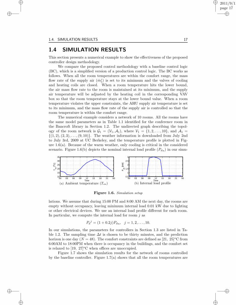
The numerical example considers a network of 10 rooms. All the rooms havethe same model parameters as in Table 1.1 identified for the conference room inthe Bancroft library in Section 1.2. The undirected graph describing the topol-ogy of the room network is G1 = (V1,A1), where V1 = {1, 2, . . . , 10}, and A1 ={(1, 2), (2, 3), . . . , (9, 10)}. The weather information is downloaded from July 2ndto July 3rd, 2009 at UC Berkeley, and the temperature profile is plotted in Fig-ure 1.6(a). Because of the warm weather, only cooling is critical in the consideredscenario. Figure 1.6(b) depicts the nominal internal load profile (Pdn) in our simu-

00 03 06 09 12 15 18 21 0010

15

20

25

30

35

Toa

[o C]

Time(a) Ambient temperature (Toa)

00 03 06 09 12 15 18 21 000.5

1

1.5

2

2.5

3

Pdn

[kW

]

Time(b) Internal load profile

Figure 1.6. Simulation setup

lations. We assume that during 15:00 PM and 8:00 AM the next day, the rooms areempty without occupancy, leaving minimum internal load 0.01 kW due to lightingor other electrical devices. We use an internal load profile different for each room.In particular, we compute the internal load for room j as

Pdj = (1 + 0.2j)Pdn, j = 1, 2, . . . , 10.

In our simulations, the parameters for controllers in Section 1.3 are listed in Ta-ble 1.2. The sampling time ∆t is chosen to be thirty minutes, and the predictionhorizon is one day (N = 48). The comfort constraints are defined as [21, 25]oC from6:00AM to 18:00PM when there is occupancy in the buildings, and the comfort setis relaxed to [19, 27]oC when offices are unoccupied.

Figure 1.7 shows the simulation results for the network of rooms controlledby the baseline controller. Figure 1.7(a) shows that all the room temperatures are


i

i

i

i

i

i

i

i


Table 1.2. Parameters for the numerical example

param value param value param value param valuem 0.005 kg/s m 5 kg/s ηc 0.7 ηh 0.8∆Tc 0 K ∆Tc 8 K Pf 0.08 α 0.25∆Th 0 K ∆Th 8 K δ 0 δ 0.8COPc 5 COPh 0.9 N 48 κ 5× 10−3

within the comfort range defined by the dotted lines. During early morning till04:00 am, all zone temperatures are within the comfort range. As a result, thesupply fan only maintains the minimum required air mass flow rate to each zone,and the valve of the cooling coils in the AHU is fully closed. The occupancy loadat noon results in a peak total air mass flow rate of 2.8 kg/s. The cooling coils areoperating at maximum capacity as soon as one of the zone temperatures hits theupper constraints so that the thermal comfort can be guaranteed. The return airdamper position is fully closed to take advantage of free cooling when the ambienttemperature is lower than the zone temperature.

The performance of proposed DMPC controller is reported in Figure 1.8. Itcools down the room temperature to the lower bounds of the comfort range duringthe early morning (Figure 1.8(a)) while the baseline controller remains inactivateduntil the room temperature hits the upper bounds around 4:00 AM (Figure 1.7(a)).This precooling saves energy, since during the early morning the lower ambienttemperature enables free cooling. The free cooling is illustrated in Figure 1.8(d).The MPC algorithm decides to open the cooling coil valve from 7:00 am, which is twohours later than the schedule proposed by baseline control logics in Figure 1.7(d).

Moreover, it is noted that instead of cooling all zones simultaneously, MPCcools down zones consecutively as Figure 1.8(a) illustrates. This feature significantlyreduces the peak total air flow rate from 7.1 kg/s of BC to 5.2 kg/s (Figure 1.8(b)),and thus saves fan energy consumption (note that we use a quadratic penalty oftotal supply air mass flow rate in (1.10a)). The simulation results suggested thatthe pre-cooling and consecutive cooling strategies induced by DMPC enable a 40.5%energy saving compared to the baseline.

DMPC Algorithm Complexity

The proposed DMPC Algorithm 1.1 can be implemented in a network of embed-ded processors with low computational capacity since Steps 3 and Steps 4 of Algo-rithm 1.1 require only a few algebraic operations and simple projections. Figure 1.10shows that a large number of iterations is required. This imposes a lower-bound onthe necessary network communication speed.

The DMPC Algorithm 1.1 was coded in Matlab R© and runs on a single PCwith Intel Core Duo CPU 3.00GHz. The runtime of the DMPC algorithm is es-timated based on the assumption that the computation of Step 3 and Step 4 inAlgorithm 1.1 are executed in parallel on Nv +1 units including the controller unitsequipped on each VAV box and the AHU unit, and that the communication time is


i

i

i

i

i

i

i

i

1.4. SIMULATION RESULTS 19

00 03 06 09 12 15 18 21 00

18

20

22

24

26

28zo

ne te

mpe

ratu

re [° C

]

(a) Room temperature (T j)

00 03 06 09 12 15 18 21 000

2

4

6

Mas

s flo

w r

ate

[kg/

s]

Total mass flow rate

(b) Mass flow rate of the supply air from

VAV box (˙

mjs)

00 03 06 09 12 15 18 21 00

0

0.5

1

retu

rn d

ampe

r po

sitio

n

(c) Return air damper position (δ)

00 03 06 09 12 15 18 21 000

2

4

6

8

cool

ing

coil

[o C]

(d) Temperature difference across coolingcoil (∆Th)

Figure 1.7. System behavior

for simplified baseline control logics

00 03 06 09 12 15 18 21 00

18

20

22

24

26

28

zone

tem

pera

ture

[° C]

(a) Room temperature (T j)

00 03 06 09 12 15 18 21 000

2

4

6

Mas

s flo

w r

ate

[kg/

s]

Total mass flow rate

(b) Mass flow rate of the supply air from

VAV box (˙

mjs)

00 03 06 09 12 15 18 21 00

0

0.5

1

retu

rn d

ampe

r po

sitio

n

(c) Return air damper position (δ)

00 03 06 09 12 15 18 21 000

2

4

6

8

cool

ing

coil

[o C]

(d) Temperature difference across coolingcoil (∆Th)

Figure 1.8. System behavior

for distributed model predictive control

neglected. The results are reported in Figure 1.12 for different numbers of thermalzones considered. The red dashed line shows the runtime of DMPC algorithm whenimplemented on Nv + 1 CPUs in parallel, and the black solid line depicts the timerequired to solve Problem (1.10) by Interior Point OPTimizer (IPOPT) [4] on oneCPU. One can notice that when the number of zones is less than seven, IPOPT isfaster than DMPC on a single PC. As the number of zones and the size of prob-


i

i

i

i

i

i

i

i


5 10 15 20

1

1.5

2

Number of zones

Cos

t var

iatio

ns (

%)

Figure 1.9. Cost variations

(J?DMPC − J?

IPOPT )/J?IPOPT .

0 50 100 150 200 250 30010

3

104

105

SQP subproblems number

Iter

num

ber

of L

evel

3

Figure 1.10. Number of dual

decomposition iterations at time t = 0.

lem (1.10) increase, one can notice that DMPC could be implemented with a fastercontrol sampling rate than IPOPT.

Figure 1.9 plots the variations of the optimal cost J?DMPC obtained by Al-

gorithm 1.1 relative to the optimal cost J?IPOPT by IPOPT when solving MPC

problem (1.10) with different number of zones Nv. It is noted that DMPC resultsin slightly higher optimal costs than IPOPT. The reasons for this include the omis-sion of off-diagonal terms of the hessian matrix in the modified SQP procedure, andthe selection of convergence tolerance κ in Table 1.2.

Fast Gradient Method Improvement

The advantage of applying the fast gradient method instead of the classical gradientmethod in level 3 of the DMPC scheme is illustrated in Figure 1.11. We focus onthe MPC problem (1.10) at t = 0. The modified SQP algorithm converged in 301steps. The dashed line in Figure 1.11 depicts the total number of iterations

∑np

i=1 nid

required to solve the subproblems generated from the SQP algorithm when the fastgradient method in Section 1.3.3 is applied. The solid line depicts the number ofiterations for the classical gradient method with constant step size.

In this work, nid is the number of iterations to solve the i-th subproblem (1.13)

obtained in the proximal minimization level. The number of iterations required tosatisfy the stopping criterion is, on average, about 20 times less than the classicalgradient methods.

0 50 100 150 200 250 30010

3

104

105

106

107

SQP subproblems number

Iter

num

ber

of L

evel

3

Fast gradient methodClassical gradient method

Figure 1.11. Number of dual

decomposition iterations at time t = 0.

5 10 15 200

20

40

60

80

100

120

140

Number of zones

Sol

ver

time

[s]

DMPCIPOPT

Figure 1.12. Comparison be-

tween CPU time for DMPC and IPOPT.


i

i

i

i

i

i

i

i

1.5. CONCLUSIONS 21

1.5 CONCLUSIONSIn this study a simplified two-mass room model is presented. Validation resultsshow that the model captures the thermal dynamics of a thermal zone with negligi-ble external load. Based on this model and predictive information of thermal loadsand weather, a distributed model predictive control is designed to regulate ther-mal comfort while minimizing energy consumption. We have present a three-leveliterative algorithm for the solution of the nonlinear MPC problem. The resultingscheme is suitable for being implemented on set of distributed low-cost processors.Simulation results show interesting behavior and fast computational time.


i

i

i

i

i

i

i

i



i

i

i

i

i

i

i

i

Bibliography

[1] F. Allgower, T.A. Badgwell, S.J. Qin, J.B. Rawlings, and S.J. Wright. Non-linear predictive control and moving horizon estimation - and introductoryoverview. Springer Berlin/Heidelberg, 1999.

[2] Y. Ma G. Anderson and F. Borrelli. A distributed predictive control approachto building temperature regulation. In 2011 American Control Conference,Jun. 2011.

[3] D. P. Bertsekas and J. N. Tsitsiklis. Parallel and Distributed Computation,volume 290. Springer-Verlag, Englewood Cliffs, NJ, 1989.

[4] L. Biegler and V. Zavala. Large-scale nonlinear programming using ipopt: Anintegrating framework for enterprise-wide dynamic optimization. Computers& Chemical Engineering, 33(3):575–582, 2009.

[5] F. Borrelli. Constrained Optimal Control of Linear and Hybrid Systems, volume290. Springer-Verlag, 2003.

[6] F. Borrelli, T. Keviczky, and G.E. Stewart. Decentralized constrained optimalcontrol approach to distributed paper machine control. In Decision and Con-trol, 2005 and 2005 European Control Conference. CDC-ECC ’05. 44th IEEEConference on, pages 3037 – 3042, Dec. 2005.

[7] R.J. Chillar and R.J. Liesen. Improvement of the ASHRAE secondary HVACtoolkit simple cooling coil model for simulation. Proceedings of the SimBuild2004 Conference, Boulder, Colorado., August 2004.

[8] S.P. Han. A globally convergent method for nonlinear programming. Journalof Optimization Theory and Applications, 22(3):297–309, July 1977.

[9] G.P. Henze, C. Felsmann, and G. Knabe. Evaluation of optimal control foractive and passive building thermal storage. International Journal of ThermalSciences, 43(2):173 – 183, 2004.

[10] G.P. Henze, M. Krarti, and M.J. Brandemuehl. Guidelines for improved per-formance of ice storage systems. Energy and Buildings, 35(2):111 – 127, 2003.

23


i

i

i

i

i

i

i

i

24 Bibliography

[11] G.P. Henze, J. Pfafferott, S. Herkel, and C. Felsmann. Impact of adaptivecomfort criteria and heat waves on optimal building thermal mass control.Energy and Buildings, 39(2):221 – 235, 2007.

[12] J. Jang. System Design and Dynamic Signature Identification for IntelligentEnergy Management in Residential Buildings. PhD thesis, University of Cali-fornia at Berkeley, 2008.

[13] B. Johansson, A. Speranzon, M. Johansson, and K.H. Johansson. Dis-tributed model predictive consensus. Technical report, Automatic ControlLab, School of Electrical Engineering, Royal Institute of Technology (KTH).http://citeseerx.ist.psu.edu/viewdoc/summary?doi=10.1.1.64.4190.

[14] L.S. Lasdon. Duality and decomposition in mathematical programming. Sys-tems Science and Cybernetics, IEEE Transactions on, 4(2), Jul 1968.

[15] J.H. Lee, M. Morari, and C.E. Garcia. State-space interpretation of ModelPredictive Control. IFAC, 1992.

[16] Y. Ma, F. Borrelli, B. Hencey, B. Coffey, S. Bengea, and P. Haves. Model pre-dictive control for the operation of building cooling systems. In 2010 AmericanControl Conference, pages 5106 –5111, Jun. 2010.

[17] D.Q. Mayne, J.B. Rawlings, C.V. Rao, and P.O.M. Scokaert. Constrainedmodel predictive control: Stability and optimality. Automatic, 36(6):789–814,June 2000.

[18] J.M. McQuade. A system approach to high performance buildings. Technicalreport, United Technologies Corporation, Feb. 2009. http://gop.science.house.gov/Media/hearings/energy09/april28/mcquade.pdf.

[19] Y. Nesterov. Introductory lectures on convex optimization: a basic course.2004.

[20] J. Nocedal and S. J. Wright. Numerical Optimization, chapter 18. Springer-Verlag, 1999.

[21] F. Oldewurtel, A. Parisio, C.N. Jones, M. Morari, D. Gyalistras, M. Gwerder,V. Stauch, B. Lehmann, and K. Wirth. Energy efficient building climate controlusing stochastic model predictive control and weather predictions. In 2010American Control Conference, pages 5100–5105, Jun 2010.

[22] A. Rantzer. Dynamic dual decomposition for distributed control. In AmericanControl Conference, 2009, pages 884 –888, Jun. 2009.

[23] J. B. Rawlings and B. T. Stewart. Coordinating multiple optimization-basedcontrollers: New opportunities and challenges. Journal of Process Control,18(9):839 – 845, 2008.


i

i

i

i

i

i

i

i

Bibliography 25

[24] S. Richter, M. Morari, and C.N. Jones. Towards computational complexitycertification for constrained mpc based on lagrange relaxation and the fastgradient method. In Proc. 50th IEEE Conf. on Decision and Control, Dec.2011.

[25] F.E. Romie. Transient response of the counterflow heat exchanger. Journal ofHeat Transfer, 106(3):620–626, 1984.

[26] B.T. Stewart, A.N. Venkat, J.B. Rawlings, S.J. Wright, and G. Pannocchia.Cooperative distributed model predictive control. Systems & Control Letters,July 2010.

[27] Y.W. Wang, W.J. Cai, Y.C. Soh, S.J. Li, L. Lu, and L. Xie. A simplifiedmodeling of cooling coils for control and optimization of hvac systems. EnergyConversion and Management, 45(18-19):2915 – 2930, 2004.

list of contributors - francesco borrelli · distributed model predictive control for building...

Documents