Liquidity Risk and Classical Option PricingTheory

Robert A. Jarrow∗

July 21, 2005

Abstract

The purpose of this paper is to review the recent derivatives secu-rity research involving liquidity risk and to summarize its implications forpractical risk management. The literature supports three general conclu-sions. The first is that the classical option price is "on average" true, evengiven liquidity risk. Second, it is well known that although the classical(theoretical) option hedge can not be applied as theory prescribes, itsdiscrete approximations often provide reasonable approximations. Thesediscrete approximations are also consistent with upward sloping supplycurves. And, third, risk management measures like value-at-risk (VaR)are biased low due to the exclusion of liquidity risk. A simple adjustmentfor incorporating liquidity risk into standard risk measures is provided.

1 IntroductionThis paper studies liquidity risk and its relation to classical option pricing the-ory for practical risk management applications. Classical option pricing theoryis formulated under two simplifying assumptions. One assumption is that mar-kets are frictionless and the second assumption is that markets are competitive.A frictionless market is one where there are no transactions costs, no bid/askspreads, no taxes and no restrictions on trades or trading strategies. For exam-ple, one can trade infinitesimal amounts of a security, continuously, for as longor as short a time interval as one wishes. A competitive market is one where theavailable stock price quote is good for any sized purchase or sale, alternativelystated, there is no quantity impact on the price received/paid for a trade. Bothassumptions are idealizations and not satisfied in reality. Both assumptions arenecessary for classical option pricing theory, e.g. the Black-Scholes option pric-ing model. The question arises: how does classical option pricing theory changewhen these two simplifying assumptions are relaxed? The purpose of this paperis to answer this question, by summarizing my research that relaxes these two

∗Johnson Graduate School of Management, Cornell University, Ithaca, NY, 14853 andKamakura Corporation, email: raj15@cornell.edu.

1

assumptions, see Jarrow [12], [13], Cetin, Jarrow, Protter [4], Cetin, Jarrow,Protter, Warachka [5], and Jarrow and Protter [15],[16]. The relaxation of thesetwo assumptions is called liquidity risk.Alternatively stated, liquidity risk is that increased volatility that arises

when trading or hedging securities due to the size of the transaction itself.When markets are calm and the transaction size is small, liquidity risk is small.In contrast, when markets are experiencing a crisis or the transaction size issignificant, liquidity risk is large. This quantity impact on price can be dueto asymmetric information (see Kyle [19], Glosten and Milgrom [9]) or an im-balance in demand/inventory (see Grossman and Miller [10]). It implies thatdemand curves for securities are downward sloping and not horizontal, as inclassical option pricing theory. But, classical option pricing theory has beensuccessfully used in risk management for over 20 years (see Jarrow [14]). Inlight of this success, is there any reason to modify classical option pricing the-ory? The answer is yes! Although successfully employed in some asset classesthat trade in liquid markets (e.g. equity, foreign currencies and interest rates),it works less well in others (e.g. fixed income securities and commercial loans).Understanding the changes to the classical theory due to the relaxation of thisstructure will enable more accurate pricing and hedging of derivative securitiesand more precise risk management.Based on my research, there are three broad conclusions that one can draw

with respect to liquidity risk and classical option pricing theory. The first isthat the classical option price is "on average" true, even given liquidity risk."On average" because the classical price lies between the buying and sellingprices of an option in a world with liquidity risk. In some sense, the classicaloption price is the mid-market price. Second, it is well known that althoughthe classical (theoretical) hedge1 can not be applied as theory prescribes, itsdiscrete approximations often provide reasonable approximations (see Jarrowand Turnbull [17]). These discrete approximations can, in fact, be viewed asadhoc adjustments for liquidity risk. Their usage is also consistent with upwardsloping supply curves. And, third, risk management measures like value-at-risk (VaR) do need to be adjusted to reflect liquidity risk. The classical VaRcomputations are biased low due to the exclusion of liquidity risk, significantlyunderestimating the risk of a portfolio. Fortunately, simple adjustments forliquidity risk to risk measures like VaR are available.The rest of the paper justifies, documents and explains the reasons for these

three conclusions. An outline for this paper is as follows. Section 2 presents thebasic model structure for handling liquidity risk. Sections 3 discusses arbitragefree markets and derivative pricing. Feasible trading strategies are studied insection 4. Section 5 investigates risk measures like VaR, and section 6 concludes.

1This implies trading both continuously in time and in continuous increments of shares.

2

2 The Basic ModelTo study liquidity risk in option pricing theory, we need to consider two assets: adefault free or riskless money market account and an underlying security, calleda stock. The money market account earns continuously compounded interest atthe default free spot rate, denoted rt at time t. The account starts with a dollarinvested at time 0 , B(0) = 1, and grows to B(T ) = e

T0rsds at time T . For

simplicity, we assume that there is no liquidity risk associated with investmentsin the money market account. In contrast, the stock has liquidity risk. This canbe captured via a supply curve for the stock that depends on the size of a trade.Let S(t, x) be the stock price paid/received per share at time t for a trade ofsize x.2 If x > 0 then the stock is purchased. If x < 0, the stock is sold. Thezeroth trade x = 0 is special. It represents the marginal trade (an infinitesimalpurchase or sale). On this supply curve, therefore, the price S(t, 0) correspondsto the stock price in the classical theory.We assume that the supply curve is upward sloping, that is, as x increases,

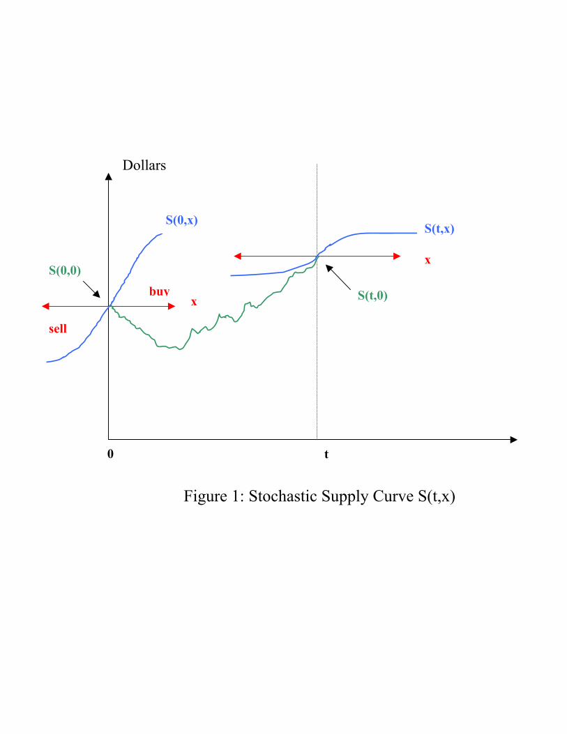
S(t, x) increases. The larger the purchase order, the higher the average pricepaid per share. An upward sloping supply curve for shares is consistent withasymmetric information in stock markets (see Kyle [19], Glosten and Milgrom[9]). Indeed, the market responds to potential informed trading by selling athigher prices and buying at lower ones. An upward sloping supply curve isgraphed in Figure 1 at time 0. The time 0 supply curve is shown on the left ofthe diagram.Although most practitioners will accept an upward sloping supply curve as

self-evident, there has been some debate on this issue in the academic literature,called the price pressure hypothesis (see Scholes [20], Shleifer [21], Harris andGruel [11]). The term "price pressure" captures the notion that buying orselling exerts either upward or downward pressure on the price, resulting in aprice change. The evidence supports the price pressure hypothesis. A recentempirical validation for an upward sloping supply curve can be found in Çetin,Jarrow, Protter and Warachka [5].One of their tests is reproduced here for emphasis in Table 1. Using the TAQ

database, Çetin, Jarrow, Protter and Warachka chose five well known companiestrading on the NYSE with varying degrees of liquidity: General Electric (GE),International Business Machines (IBM), Federal Express (FDX), Reebok (RBK)and Barnes & Noble (BKS). The time period covered was a four year periodwith 1,011 trading days, from January 3, 1995 to December 31, 1998. The leftside of Table 1 gives the implications of an upward supply curve when bothtime and information are fixed. The price inequalities indicate the ordering oftransaction prices given different size trades. For example, sales should transactat lower prices then do purchases; and small buys should have lower pricesthen do large buys. To approximate this set of inequalities, they look at asequence of transactions keeping the change in time small (the time between

2All technical details regarding the model structure (smoothness conditions, integrabilityconditions, etc.) are delegated to the references.

3

consecutive transactions). Despite the noise introduced by a small change intime (and information), the hypothesized inequalities are validated in all cases.This Table supports the upward sloping supply curve formulation.The supply curve is also stochastic. It fluctuates randomly through time, its

shape changing, although always remaining upward sloping. When markets arecalm, the curve will be more horizontal. When markets are hectic, the curvewill be more upward tilted. A possible evolution for the supply curve is givenin Figure 1. The supply curve at time t represents a more liquid market thanat time 0 because it’s less upward sloping. As depicted, the marginal stockprice’s evolution is graphed as well between time 0 and time t. This evolutionis what is normally modeled in the classical theory. For example, in the BlackScholes model, S(t, 0) follows a geometric Brownian motion. The difference hereis that when studying liquidity risk, the entire supply curve and its stochasticfluctuations across time need to be modeled.There is an important implicit assumption in this model formulation that

needs to be highlighted. In the evolution of the supply curve (as illustrated inFigure 1), the impact of the trade size on the price process is temporary. That is,the future evolution of the price process for t > 0 does not depend on the tradesize executed at time 0. This is a reasonable hypothesis. The alternative is thatthe price process for t > 0 depends explicitly on the trade size executed at time0. This happens, for example, when there are large traders whose transactionspermanently change the dynamics of the stock price process. In this situation,market manipulation is possible, and option pricing theory changes dramatically(see Bank and Baum [1], Cvitanic and Ma [7], and Jarrow [12],[13]). Marketmanipulation manifests a breakdown of financial markets, and this extreme formof liquidity risk is not discussed further herein, but left to the cited references.Suffice it to say that the three conclusions mentioned in the introduction withrespect to liquidity risk fail in these extreme market conditions. This paper onlystudies liquidity risk in well-functioning markets.Given trading in the stock and a money market account, we also need to

briefly discuss the meaning of a portfolio’s "value." The word "value" is inquotes because when prices depend on trade sizes, there is no unique value fora portfolio. To see this, consider a portfolio consisting of n shares of the stockand m shares of the money market account at time 0. The value of the portfoliois uniquely determined by the time 0 stock price, but which stock price shouldbe selected from the supply curve? There are an infinite number of choicesavailable, each corresponding to a particular point on the supply curve. Someeconomic meaningful selections are apparent. For example, the value of theportfolio if liquidated at time 0 is

liquidation value: nS(0,−n) +mB(0). (1)

Note that in the stock price, the price for selling n shares is used. Another choiceis themarked-to-market value, defined by using the price from the marginal trade(zero trade size), i.e.

marked-to-market value: nS(0, 0) +mB(0). (2)

4

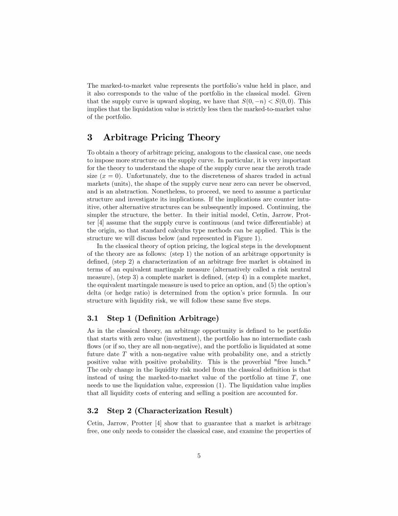
The marked-to-market value represents the portfolio’s value held in place, andit also corresponds to the value of the portfolio in the classical model. Giventhat the supply curve is upward sloping, we have that S(0,−n) < S(0, 0). Thisimplies that the liquidation value is strictly less then the marked-to-market valueof the portfolio.

3 Arbitrage Pricing TheoryTo obtain a theory of arbitrage pricing, analogous to the classical case, one needsto impose more structure on the supply curve. In particular, it is very importantfor the theory to understand the shape of the supply curve near the zeroth tradesize (x = 0). Unfortunately, due to the discreteness of shares traded in actualmarkets (units), the shape of the supply curve near zero can never be observed,and is an abstraction. Nonetheless, to proceed, we need to assume a particularstructure and investigate its implications. If the implications are counter intu-itive, other alternative structures can be subsequently imposed. Continuing, thesimpler the structure, the better. In their initial model, Cetin, Jarrow, Prot-ter [4] assume that the supply curve is continuous (and twice differentiable) atthe origin, so that standard calculus type methods can be applied. This is thestructure we will discuss below (and represented in Figure 1).In the classical theory of option pricing, the logical steps in the development

of the theory are as follows: (step 1) the notion of an arbitrage opportunity isdefined, (step 2) a characterization of an arbitrage free market is obtained interms of an equivalent martingale measure (alternatively called a risk neutralmeasure), (step 3) a complete market is defined, (step 4) in a complete market,the equivalent martingale measure is used to price an option, and (5) the option’sdelta (or hedge ratio) is determined from the option’s price formula. In ourstructure with liquidity risk, we will follow these same five steps.

3.1 Step 1 (Definition Arbitrage)

As in the classical theory, an arbitrage opportunity is defined to be portfoliothat starts with zero value (investment), the portfolio has no intermediate cashflows (or if so, they are all non-negative), and the portfolio is liquidated at somefuture date T with a non-negative value with probability one, and a strictlypositive value with positive probability. This is the proverbial "free lunch."The only change in the liquidity risk model from the classical definition is thatinstead of using the marked-to-market value of the portfolio at time T , oneneeds to use the liquidation value, expression (1). The liquidation value impliesthat all liquidity costs of entering and selling a position are accounted for.

3.2 Step 2 (Characterization Result)

Cetin, Jarrow, Protter [4] show that to guarantee that a market is arbitragefree, one only needs to consider the classical case, and examine the properties of

5

the marginal stock price process S(t, 0). In particular, they prove the followingresult.

Theorem 1 If there exists an equivalent probability Q such that S(t, 0)/B(t) isa martingale, then the market is arbitrage free.

The intuition for the theorem is straightforward. If there are no arbitrageopportunities when trading with zero liquidity impact (at the zeroth trade),then trading with liquidity can create no arbitrage opportunities that otherwisedid not exist. Indeed, the trade size impact on the price always works againstthe trader, decreasing his returns, and decreasing any potential payoffs.This theorem is an important insight. It implies that all the classical stock

price processes can still be employed in the analysis of liquidity risk, but theynow represent the zeroth point on the supply curve’s evolution. For example,an extended Black-Scholes economy is given by the supply curve

S(t, x) = S(t, 0)eαx (3)

where α > 0 is a constant and S(t, 0) is a geometric Brownian motion. That is,

dS(t, 0) = µS(t, 0)dt+ σS(t, 0)dWt (4)

where µ, σ > 0 are constants andWt is a standard Brownian motion. The supplycurve in expression (3) depends on the trade size x in an exponential manner.Indeed, as x increases, the purchase price increases by the proportion eαx. Thissimple supply curve, as a first approximation, appears to be consistent with thedata (see Cetin, Jarrow, Protter, Warachka [5]). A typical value of α lies in theset [.00005, .00015], i.e. between 0.5 and 1.5 basis points per transaction is atypical quantity impact on the price (see Cetin, Jarrow, Protter, Warachka [5],Table 1).Since we know that a geometric Brownian motion process in the classical

case admits no arbitrage, this theorem tells us that the supply curve extensionadmits no arbitrage as well. We will return to this example numerous times inthe subsequent text to illustrate the relevant insights.

3.3 Step 3 (Definition Market Completeness)

As in the classical case, a complete market is defined to be a market where(dynamically) trading in the stock and money market account can reproducethe payoff to any derivative security at some future date. The same definitionapplies with supply curves, although in attempting to reproduce the payoffto a derivative security, the actual trade size determined price must be used.Otherwise, the definition is identical.Unfortunately, one can show that in the presence of a supply curve, if the

market was complete in the classical case (for the marginal price process S(t, 0)),it will not be complete with liquidity costs. The reason is that part of theportfolio’s value evaporates due to the liquidity cost in the attempt to replicatethe option.

6

But, recall that in the classical case, the completeness result for the priceprocess requires that the replicating strategy often involves continuous trading ofinfinitesimal quantities of a stock in an erratic fashion3. Of course, in practice,following such a replicating strategy is impossible. And, only approximatingtrading strategies can be employed that involve trading at discrete time intervals(see Jarrow and Turnbull [17] for a more detailed explanation). Thus, in theclassical model, the best we can really hope for (in practice) is an approximatelycomplete market. That is, a market that can approximately reproduce the payoffto any derivative security at some future date.It turns out that under the supply curve formulation, Cetin, Jarrow, Protter

[4] prove the following theorem.

Theorem 2 Given the existence of an equivalent martingale measure (as inTheorem 1), if it is unique, then the market is approximately complete.

In the classical case, if the equivalent martingale measure is unique, thenthe market is complete. Here, almost the same result holds when applied tothe marginal stock price process S(t, 0). The difference is that one only gets anapproximately complete market. The result follows because there always existtrading strategies, involving quick trading of small quantities, that incur verylittle price impact costs (since one is trading nearly zero shares at all times). Byreducing the size of each trade, but accumulating the same aggregate quantityby trading more quickly, one can get arbitrarily close to the no liquidity costcase.Again, the importance of this theorem for applications is that all of the

classical stock price process results can still be employed in the analysis ofliquidity risk. Indeed, if the classical stock price process is consistent with acomplete market, then it will imply an approximately complete market givenliquidity costs. For example, returning to the extended Black-Scholes economypresented above in expression (3), since we know in the classical case that itimplies a complete market, this theorem tells us that the supply curve extensionimplies an approximately complete market as well.

3.4 Step 4 (Pricing Options)

Just as in the classical case, one can show that in an approximately completemarket, the value of an option is its discounted expected payoff using the mar-tingale measure in taking the expectation. The martingale measure adjusts thatstatistical (or actual) probabilities to account for risk (see Jarrow and Turnbull[17] for a proof of these statements). For concreteness, let CT represent thepayoff to an option at time T . For example, if the option is a European callwith strike price K and maturity T , then CT = max[S(T, 0) − K, 0]. In thepayoff of this European call, the marginal stock price is used (at the zerothtrade size). The reason is that (as explained in step 3) the replicating trading

3By "erratic" I mean similar to the path mapped out by a Brownian motion.

7

strategy avoids (nearly) all liquidity costs. This is reflected in the option’s pay-off by setting the trade size x = 0. For more discussion on this point, see Cetin,Jarrow, Protter [4].Given this payoff, the price of the option at time 0 is given by

C0 = E(CT e− T

0rsds) (5)

where E(·) represents expectation under the martingale measure. This is thestandard formula used to price options in the classical case.Continuing our European call option with strike price K and maturity T

example, let us assume that the stock price supply curve evolves according tothe extended Black-Scholes economy as in expression (3) above, and that thespot rate of interest is a constant, i.e. rt = r for all t. Then, the pricing formulabecomes:

C0 = E(max[S(T, 0)−K, 0]e−rT )

= S(0, 0)N(h(0))−Ke−rTN(h(0)− σ√T ) (6)

where σ > 0 is the stock’s volatility, N(·) is the standard cumulative normaldistribution function, and

h(t) ≡ logS(t, 0)− logK + r(T − t)

σ√T − t

+σ

2

√T − t.

This is the standard Black Scholes formula, but in a world with liquidity risk!

3.5 Step 5 (Replication)

In the classical case, the replicating portfolio can often be obtained from the val-uation formula by taking its first partial derivative with respect to the underlyingstock’s time 0 price. For example, with respect to the classical Black-Scholesformula in expression (6) above, the hedge ratio is the option’s delta and it isgiven by

∆t =∂Ct

∂S(t, 0)= N(h(t)) (7)

for an arbitrary time t.This represents the number of shares of the stock to hold at time t to replicate

the payoff to the European call option with strike price K and maturity T .The holdings in the stock must be changed continuously in time according toexpression (7), buying and selling infinitesimal shares of the stock to maintainthis hedge ratio.In the situation with an upward sloping supply curve, this procedure for

determining the replicating portfolio is almost the same. The difference is thatthe classical replicating strategy will often be too erratic, and a smoothingof the replicating strategy will need to be employed to reduce price impactcosts. The exact smoothing procedure is detailed in Cetin, Jarrow, Protter[4]. Consequently, the classical hedge (appropriately smoothed) provides anapproximate replicating strategy for the option. For the Black Scholes extended

8

economy that we have been discussing, the smoothed hedge ratio for any timet is given by

∆t = 1[ 1n ,T− 1n )(t)n

Z t

(t− 1n )

+

N(h(u))du, if 0 ≤ t ≤ T − 1n

(8)

∆t = (nT∆(T− 1n )− n∆(T− 1

n )t), if T − 1

n≤ t ≤ T.

where 1[ 1n ,T− 1n )(t) is an indicator function for the time set [ 1n , T − 1

n) and n isthe step size in the approximating procedure. As evidenced in this expression,the smoothing procedure is accomplished by taking an integral (an averagingoperation). The approximation improves as n→∞.In summary, as just documented, the classical approach almost applies. But,

there is a potential problem with the smoothed trading strategy. Just as in theclassical case, it usually involves continuous trading of infinitesimal quantities ofthe stock’s shares, which is impossible in practice. And, just as in the classicalcase, to make the hedging theory consistent with practice we need to restrictourselves to more realistic trading strategies. This is the subject of the nextsection.

4 Feasible Replicating StrategiesThe implication of Cetin, Jarrow, Protter [4] is that the classical option pricemust hold in the extended supply curve model. Taken further, this implies thatoption markets should exhibit no quantity impact on prices, no bid/ask spreads,even if the underlying stock price curve does! This is a counter-intuitive impli-cation of the model, directly due to the ability to trade continuously in time ininfinitesimal quantities. Just as in the classical model, if one removes continu-ous trading strategies, and only admits discrete trading, then this implicationchanges.Cetin, Jarrow, Protter, Warachka [5] explore this refinement. Cetin, Jarrow,

Protter, Warachka reexamine the upward sloping supply curve model consid-ering only discrete trading strategies. Discrete trading strategies only allow afinite number of trades (at random times) in any finite time interval. As onemight expect, the situation becomes analogous to a market with transactioncosts. Fixed (or proportionate) transaction costs, due to their existence, pre-clude the existence of continuous trading strategies, otherwise transaction costswould become infinite in any finite time (see Barles and Soner [2], Cvitanic andKaratzas [6], Cvitanic, Pham, Touze [8], Jouini and Kallal [18], Soner, Shreveand Cvitanic [22], and Jarrow and Protter [16]). Hence, many of the insightsfrom the transaction cost literature can now be directly applied to Cetin, Jarrow,Protter, Warachka’s market.In such a market, one can not exactly or even approximately replicate an

option. The market is incomplete. This is due to the fact that transactioncosts evaporate value from a portfolio. Consequently, one seeks to determine

9

the cheapest buying price and the largest selling price for an option. If theoptimal super- or sub- replicating strategy can be determined, then one gets arelationship between the buying and selling prices, and the classical price:

Csell0 ≤ Cclassical

0 ≤ Cbu y0 . (9)

The classical price lies between the buying and selling prices obtainable by super-and sub- replication. In this sense, the classical option price is the "average" ofthe buying and selling prices. This statement provides the justification for thefirst conclusion contained in the introduction.To get a sense for the percentage magnitudes of the liquidity cost band

around the classical price, Table 2 contains some results from Cetin, Jarrow,Protter, Warachka [5] where they document the liquidity costs associated withthe extended Black-Scholes model given in expression (3) above given only dis-crete trading is allowed. As a percentage of the option’s price, liquidity costsusually are less than 100 basis points.Unfortunately, the optimal strategy for buying (or selling) is often difficult

to obtain, because it involves solving a complex dynamic programming problem.For this reason, practical replicating strategies often need to be used instead.For example, the standard Black Scholes delta hedge, implemented once a day(instead of continuously in time), is one such possibility. Cetin, Jarrow, Protter,Warachka show that this strategy provides a reasonable approximation to theoption’s optimal buying or selling strategy. As such, these practical hedgingstrategies used by the industry can be viewed as adjustments to the classicalmodel for handling liquidity risk. This observation serves as the justification forthe second conclusion drawn in the introduction, i.e. that the discrete tradingstrategies used in practice serve as reasonable approximations to the optimaltrading strategy given liquidity costs. The third conclusion is justified in thenext section.

5 Risk Management MeasuresThe classical risk measures, like value at risk (VaR), do not explicitly incorporateliquidity risk into the calculation. Given the liquidity risk model introducedabove, a simple and robust adjustment for liquidity risk is now readily availableas detailed in Jarrow and Protter [15].As discussed in section 3 above, trading continuously and in infinitesimal

amounts enables one to avoid all liquidity costs. In actual markets, this cor-responds to slow and deliberate selling of the portfolio’s assets. But, whencomputing risk measures for risk management, one needs to be conservative.The worst case scenario is a crisis situation, where one has to liquidate assetsimmediately. The idea is that if the market is declining quickly, then one doesnot have the luxury to sell assets slowly (continuously) in “small” quantitiesuntil the entire position is liquidated. In a crisis situation, the supply curveformulation provides the relevant value to be used, the liquidation value of theportfolio from expression (1) above.

10

The liquidation value of a portfolio can be determined by estimating eachstock’s supply curve’s stochastic process, and knowing the size of each stockposition. Supply curve estimation is not a difficult exercise, see Çetin, Jarrow,Protter and Warachka [5]. For example, in the extended Black-Scholes modelof expression (3) above, a simple time series regression can be employed. Giventime series observations of transaction prices and trade sizes (S(τ i, xτ i), τ i)

Ii=1,

it can be shown that the regression equation is

ln

µS(τ i+1, xτi+1)

S(τ i, xτi)

¶= α

£xτi+1 − xτi

¤+ µ [τ i+1 − τ i] + σ τi+1, τ i . (10)

The error τi+1, τ i equals√τ i+1 − τ i with being distributed N (0, 1).4 Then,

in computing VaR one can explicitly include the liquidity discount parameter αto determine the portfolio value for immediate liquidation.The bias in the classical VaR computation can be easily understood. The

classical VaR computation uses the marked-to-market value of the portfoliogiven in expression (2). In contrast, the VaR computation including liquidityrisk should use the liquidation value given in expression (1). As noted earlier,the liquidation value in expression (1) is always less than the marked-to-marketvalue in expression (2). This implies that the classical VaR computation will bebiased low, indicating less risk in the portfolio than actually exists. This liquidityrisk adjustment to VaR based on the portfolio’s liquidation value, rather thanits marked-to-market value, yields the basis for the third conclusion stated inthe introduction.To illustrate these computations, let us again consider the extended Black

Scholes economy of expression (3). Let us consider a portfolio of N stocksi = 1, ..., N with share holdings denoted by ni in the ith stock. We denote theith stock price by

Si(t, x) = Si(t, 0)eαix. (11)

The marked-to-market value of the portfolio at time T is

NXi=1

niSi(T, 0).

The time T liquidation value is

NXi=1

niSi(T,−ni) =NXi=1

niSi(T, 0)e−αini .

When computing VaR either analytically or via a simulation, the adjustment tothe realization of Si(T, 0) is given by the term e−αini . This is an easy compu-tation.

4This is the regression equation used to obtain the typical values for α reported earlier.

11

6 ConclusionThis paper reviews the recent literature on liquidity risk for its practical use inrisk management. The literature supports three general conclusions. The firstis that the classical option price is "on average" true, even given liquidity risk.Second, it is well known that although the classical (theoretical) option hedgecan not be applied as theory prescribes, its discrete approximations often pro-vide reasonable approximations (see Jarrow and Turnbull [17]). These discreteapproximations are also consistent with upward sloping supply curves. And,third, risk management measures like value-at-risk (VaR) are biased low due tothe exclusion of liquidity risk. Fortunately, simple adjustments for liquidity riskto risk measures like VaR are readily available.

12

References[1] P. Bank and D. Baum, 2004, “Hedging and Portfolio Optimization in Illiq-

uid Financial Markets with a Large Trader,” Mathematical Finance, 14,1-18.

[2] Barles, G. and H. Soner, 1998, “Option Pricing with Transaction Costsand a Nonlinear Black-Scholes Equation,” Finance and Stochastics, 2, 369- 397.

[3] Çetin, U., 2003, Default and Liquidity Risk Modeling, Ph.D. thesis, CornellUniversity.

[4] Çetin, U., R. Jarrow, and P. Protter, 2004, "Liquidity Risk and ArbitragePricing Theory," Finance and Stochastics, 8, 311-341.

[5] Çetin, U., R. Jarrow, P. Protter and M. Warachka, 2005, “Pricing Op-tions in an Extended Black Scholes Economy with Illiquidity: Theory andEmpirical Evidence," forthcoming, The Review of Financial Studies.

[6] Cvitanic, J. and I. Karatzas, 1996, “Hedging and Portfolio Optimizationunder Transaction Costs: a Martingale Approach,” Mathematical Finance,6 , 133 - 165.

[7] Cvitanic, J and J. Ma, 1996, “Hedging Options for a Large Investor andForward-Backward SDEs,” Annals of Applied Probability, 6, 370 - 398.

[8] Cvitanic, J., H. Pham, N. Touze, 1999, “A Closed-form Solution to theProblem of Super-replication under Transaction Costs,” Finance and Sto-chastics, 3, 35 - 54.

[9] Glosten, L. and P. Milgrom, 1985, “Bid, Ask and Transaction Prices ina Specialist Market with Heterogeneously Informed Traders,” Journal ofFinancial Economics, 14 (March), 71 - 100.

[10] Grossman, S. and M. Miller, 1988, “Liquidity and Market Structure,” Jour-nal of Finance, 43 (3), 617 - 637.

[11] Harris, L. and E. Gruel, 1986, "Price and Volume Effects Associated withChanges in the S&P 500 List: New Evidence for the Existence of PricePressure," Journal of Finance, 41 (4), 617-637.

[12] Jarrow, R., 1992, “Market Manipulation, Bubbles, Corners and ShortSqueezes,” Journal of Financial and Quantitative Analysis, September, 311- 336.

[13] Jarrow, R., 1994, “Derivative Security Markets, Market Manipulation andOption Pricing,” Journal of Financial and Quantitative Analysis, 29 (2),241 - 261.

13

[14] Jarrow, R., 1999, “In Honor of the Nobel Laureates Robert C. Mertonand Myron S. Scholes: A Partial Differential Equation that Changed theWorld,” The Journal of Economic Perspectives, 13 (4), 229-248.

[15] Jarrow, R. and P. Protter, 2005, "Liquidity Risk and Risk Measure Com-putation," forthcoming, The Review of Futures Markets.

[16] Jarrow, R. and P. Protter, 2005, "Liquidity Risk and Option Pricing The-ory, forthcoming, Handbook of Financial Engineering, ed., J. Birge and V.Linetsky, Elsevier Publishers.

[17] Jarrow, R. and S. Turnbull, 2000, Derivative Securities, Southwestern Pub-lishing Co.

[18] Jouini, E. and H. Kallal, 1995, “Martingales and Arbitrage in SecuritiesMarkets with Transaction Costs,” Journal of Economic Theory, 66 (1),178 - 197.

[19] Kyle, A., 1985, “Continuous Auctions and Insider Trading,” Econometrica,53, 1315-1335.

[20] Scholes, M., 1972, "The Market for Securities: Substitution vs Price Pres-sures and the Effects on Information Share Prices," Journal of Business,45, 179-211.

[21] Shleifer, A., 1986, "Do Demand Curves for Stocks Slope Down?," Journalof Finance, (July), 579-589.

[22] Soner, H.M., S. Shreve and J. Cvitanic, 1995, “There is no NontrivialHedging Portfolio for Option Pricing with Transaction Costs,” Annals ofApplied Probability, 5, 327 - 355.

14

Dollars

Figure 1: Stochastic Supply Curve S(t,x)

sell

S(0,x)

S(0,0) buy

x

x

t

S(t,x)

S(t,0)

0

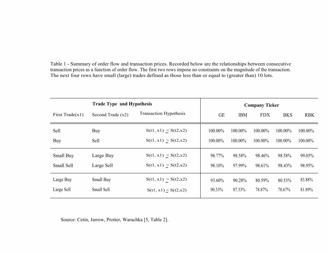
Table 1 - Summary of order flow and transaction prices. Recorded below are the relationships between consecutive transaction prices as a function of order flow. The first two rows impose no constraints on the magnitude of the transaction. The next four rows have small (large) trades defined as those less than or equal to (greater than) 10 lots.

Trade Type and Hypothesis Company Ticker

First Trade(x1) Second Trade (x2) Transaction Hypothesis GE IBM FDX BKS RBK

Sell Buy -S(t1, x1) < S(t2,x2) 100.00% 100.00% 100.00% 100.00% 100.00%

Buy Sell -S(t1, x1) > S(t2,x2) 100.00% 100.00% 100.00% 100.00% 100.00%

Small Buy Large Buy -S(t1, x1) < S(t2,x2) 98.77% 98.58% 98.46% 98.58% 99.05%

Small Sell Large Sell -S(t1, x1) > S(t2,x2) 98.10% 97.99% 98.61% 98.43% 98.95%

Large Buy Small Buy -S(t1, x1) > S(t2,x2) 93.60% 90.28% 80.59% 80.53% 83.88%

Large Sell Small Sell -S(t1, x1) < S(t2,x2) 90.33% 87.33% 78.87% 78.67% 81.89%

Source: Cetin, Jarrow, Protter, Warachka [5, Table 2].

Table 2- Summary of the liquidity costs for 10 options, each on 100 shares. For at-the-options, the strike price equals the initial stock price. The stock price is increased (decreased) by $5 for in-the-money (out-of-the-money) options.

Option Characteristics Costs Associated with Replicating Portfolio for 10 Options

Company Option Option Price Liquidity Cost Liquidity Cost Total Percentage Name Moneyness with a = 0 (at t = 0) (after t = 0) Liquidity Cost Impact

GE In 548.91 19.31 5.77 25.08 0.46

At 177.94 9.59 10.06 19.65 1.10

Out 46.94 0.86 0.82 1.68 0.36

IBM In 730.56 8.61 3.46 12.07 0.17

At 362.91 4.81 4.46 9.27 0.26

Out 229.90 2.44 2.29 4.73 0.21

FDX In 562.42 15.70 4.96 20.66 0.37

At 188.42 8.46 8.09 16.55 0.88

Out 56.07 0.92 0.87 1.79 0.32

BKS In 517.87 23.39 4.52 27.91 0.54

At 133.50 11.07 10.18 21.25 1.59

Out 12.25 0.12 0.11 0.23 0.19

RBK In 513.40 20.02 3.67 23.69 0.46

At 129.33 9.16 8.44 17.60 1.36

Out 8.36 0.05 0.05 0.10 0.12

Source: Cetin, Jarrow, Protter, Warachka [5, Table 3].