MPRAMunich Personal RePEc Archive

Liquidity and Dividend Policy

Deniz Igan and Aureo de Paula and Marcelo Pinheiro

2006

Online at http://mpra.ub.uni-muenchen.de/29409/MPRA Paper No. 29409, posted 10. March 2011 12:21 UTC

Liquidity and Dividend Policy�

Deniz Igany Áureo de Paulaz Marcelo Pinheirox

December 27, 2010

Abstract

We document the association between a �rm�s payout policy and its stock�s liquidity.

In particular, we show that dividend-paying �rms have a more liquid market for their

stock and measures of a stock�s liquidity is positively linked to its probability of being a

dividend payer. Furthermore, this link between dividends and liquidity is stronger when

shareholders are more powerful. This is consistent with a mechanism in which payout

decisions act as a commitment not to invest: by distributing cash, the �rm reduces

its potential for internal equity �nancing, raising its cost of capital and leading to less

investment. Such a mechanism may lead to less volatile stock prices and potentially

to a decrease in the adverse selection costs faced by liquidity-constrained shareholders,

increasing stock price liquidity. When shareholders have more power, liquidity would be

more strongly linked with dividends as managers would be more likely to pay dividends

to meet shareholders�preference for liquidity.

Keywords: Liquidity, Dividend Payers, Adverse Selection Costs, Corporate Gover-

nance, Shareholder Power, Informed Trading.

JEL Classi�cation: G14, G31, G35.

�We would like to thank Franklin Allen, Markus Brunnermeier, Stijn Claessens, Tom George, Frankde Jong, Pete Kyle, Natalia Piqueira, Hélène Rey, Ailsa Röell, José Scheinkman, Stuart Turnbull, WeiXiong and seminars participants at Princeton University, the University of Houston, and Midwest FinanceAssociation Meetings for insightful comments and suggestions. We would also like to thank Ronnie Sadkafor providing us with data that, albeit excluded from this version of the paper, was helpful in reinforcingour intuitions. Remaining errors are our own. The views expressed here are those of the authors and donot necessarily represent those of the IMF or IMF policy.

yCorresponding author. Mailing address: IMF - Research Dept., 700 19th Street NW, Washington, DC,20431. Phone: (202) 623-4743. Email: digan@imf.org.

zUniversity of Pennsylvania, Department of Economics. Email: aureo@econ.upenn.edu.xGeorge Mason University, School of Management. Email: mpinheir@gmu.edu.

1

I Introduction

Payout decisions have an impact but are also a¤ected by liquidity conditions of sharehold-

ers. Most straightforwardly, distributing cash to shareholders increase their cash balance,

and hence, relaxes their liquidity constraints. More interestingly, the decision to distribute

cash may have a dynamic relationship with the properties of the stock price, and hence,

the liquidity of the stock in the market place. Such a relationship could arise through

the �commitment not to invest�: distributing cash reduces the �rm�s potential for inter-

nal equity �nancing, raises the cost of external capital, and leads to less investment. In

the extreme, a �rm would pay cash out only when it envisions no worthy investment op-

portunities because internal �nancing is cheaper. With less investment and assuming cash

�ows from existing operations are always more predictable than �ows from risky investment

projects, uncertainty in payo¤s would be reduced and stock price volatility may subside,

decreasing the adverse selection costs faced by liquidity-constrained shareholders. In this

paper, we present a toy model demonstrating this mechanism and empirically analyze the

link between between payout policy and stock liquidity by adding liquidity variables to the

list of �rm characteristics that determine the propensity to pay dividends.

The novel part of the paper is the study of a corporate �nance decision taking market

microstructure elements into account. We consider a situation where shareholders�need for

liquidity is linked to the �rm�s decision to pay dividends and/or engage in share repurchases.

We think of shareholders as agents that face a trade-o¤ between expected returns and

liquidity. In equilibrium, some �rms are willing to forgo investments and accept potentially

lower growth prospects in exchange for a more liquid market for their shares and they

distribute cash.

If one interprets the decision to pay dividends as a pre-commitment to invest less in

opportunities that are riskier than its existing operations, it is easy to see that by paying

dividends a �rm may be able to reduce its earnings volatility. In a market with informed

agents, a(n uninformed) shareholder that is hit by a liquidity shock will face adverse selection

when trading. Furthermore, these adverse selection costs will be lower the less risky

2

the company is (an intuition reminiscent of Kyle (1985)). In other words, assymmetric

information about the returns will play a bigger role when the investments undertaken are

risky and the stock price, as a consequence, is more volatile. So, by paying dividends or

repurchasing shares, a company would a¤ect the volatility and liquidity of its stock. If

shareholders do indeed care about liquidity and �rms care about shareholders, we should

observe an e¤ect of liquidity on the decision to make payouts to shareholders.1

This reasoning leads to several testable conjectures. First, dividend-paying �rms have

a more liquid market. Therefore, measures of liquidity should be positively associated

with the probability that a �rm is a dividend payer. Second, payers are less volatile as

they tend to use dividends as a commitment device and not to undertake risky investments.

Accordingly, shareholders of �rms with more investment opportunities face more volatile

returns and higher adverse selection costs because of the uncertainty surrounding these

investments. Finally, increased shareholder power leads to an increase in the likelihood

that a �rm is a payer as shareholders like more liquidity.2

Our empirical analysis closely follows the work of Fama and French (2001) (FF from

now on). FF analyzes possible explanations for the decline in the number of dividend

paying �rms. They �rst identify the characteristics of dividend paying �rms, and then ask

if the decline can be explained by changes in the prevalence of these characteristics. They

argue that even after controlling for the characteristics, which include size, pro�tability,

and growth opportunities, the decline persists. In other words, the decline can be better

explained by a generalized reduction in the propensity to pay, rather than by a change in the

characteristics of �rms. We build on their work arguing that potentially important variables

were excluded from their analysis, namely liquidity measures and proxies for shareholder

power. We do not, however, concentrate so much on the reasons for the decline, but rather

on the variables that seem to be important in determining the likelihood of a �rm being a

dividend payer.

1Throughout the paper we focus on dividends but the results are also veri�ed for share repurchases.2One should think about this and the �rst implication together: Liquidity should be of greater importance

for the decision to pay dividends for �rms that have a high level of shareholder power.

3

The potential power to signal strategy and prospects to the market has been one of the

main features of dividends analyzed in the literature.3 We depart considerably from this

approach by assuming that establishing its type is not the �rm�s main or sole concern in

choosing their payout policy. Their decision of whether or not to pay dividends actually

determines the characteristics of their payo¤s. The interesting point, and the main object

of analysis in this paper, is the fact that liquidity costs generated by asymmetric information

di¤er across �rms depending on whether they are dividend payers or not. Bhattacharya

(1979) also argues that agents� liquidity needs may be related to the dividend payment

decision. However, the mechanism leading to this result is di¤erent. In Bhattacharya

(1979), agents�urgency comes from di¤ering planning horizons, while here we think of it

as coming from a shock. We focus on the interaction between the payout policy (and

the availability of funds for investments) and the liquidity costs faced by shareholders and,

consequently, the �rm�s �nal value.

Baker and Wurgler (2002a, b) analyze the impact of a measure of dividend premium

on the decision to initiate payment. They develop a stylized behavioral model to suggest

that the stock price premium carried by dividend-paying �rms explains why �rms decide to

pay or stop paying dividends and present some suggestive evidence to support their theory.

Their approach aims to explain the downward trend in the propensity to pay, hence they

concentrate on the time series dimension.4 Conversely, our approach is mostly concentrated

on the cross-section variation as we are interested in explaining the decision to pay dividends

as a function of �rm characteristics. We propose a mechanism that can shed light into the

existence of the dividend premium. Investors in need of liquidity may display a preference

for the dividend payers and this preference can show up in the form of a premium on

the dividend-paying stocks. Thus, the windfall created by shareholders� liquidity needs

would be observationally equivalent to a dividend premium changing through time. Our

results suggest that it may be the case that it is not the dividend premium that drives the

3See Bhattacharya (1979), Miller and Rock (1985), Makhija and Thompson (1986), Williams (1988),Benartzi, Michaely and Thaler (1997), and Allen and Michaely (2002), among others.

4Actually, using a variable such as dividend premium makes it impossible to use the cross-section varia-tion.

4

propensity to pay, but rather that the liquidity gains from paying drives this propensity

and at the same time leads to the dividend premium.

Benartzi, Michaely and Thaler (1997) test the information content of changes in divi-

dends with respect to the earnings of the �rm, which is a common implication in signaling

models. The question is whether the �rms are signaling a change expected to happen in

the future or a change already realized in the past. Their result that �rms are in fact

signaling the past is consistent with our �ndings. There, �rms that initiate or increase

dividends have experienced an increase in earnings, but do not show unexpected increases

in the future. Firms that cut dividends have experienced decrease in earnings in the past,

but show increases in the future. Our story also asserts that, in order to pay dividends, the

�rm needs to have had positive earnings. However, in agreement with their �ndings, these

�rms are not expected to show any further increase in pro�tability, potentially because they

are committing not to invest and potentially passing on pro�table opportunities. Similarly,

�rms that decide not to pay dividends experience a decrease in earnings since funds are

diverted to a risky investment opportunity. Again in conformity with their results, these

�rms are expected to show signi�cant increase in earnings in the future. Hence, our hy-

pothesis accords with results that have empirical support in the existing literature. Other

implications, concerning the links between dividends and liquidity as well as between div-

idends and shareholder power are new and has received little attention making this paper

one of the few documenting these relationships.

Banerjee, Gatchev, and Spindt (2007), in a coincident paper, also investigate the interac-

tion between payout policy and stock market liquidity. They, however, conclude that there

exists a negative relationship between dividends and stock market liquidity, interpreting this

as a sign that investors view dividends and liquidity as substitutes. Yet, their empirical

analysis is fragmented in the sense that all regressions are conducted in sub-samples distin-

guished by three di¤erent time periods (1963-1977, 1978-1992, 1993-2003). As we show, in

the whole sample period, the sign of the relationship is reversed. Hence, we demonstrate

that the interaction between dividends and stock market liquidity is not necessarily as it

5

is depicted elsewhere in the literature. Moreover, the main feature that distinguishes this

paper is the fact that we study an interesting channel that may have a bearing on this

relationship, namely, the potential e¤ect on investment decisions and stock price return

distribution, beyond the straightforward channel that dividends can relax shareholders�

liquidity constraints.

Harford, Mansi, and Maxwell (2008), in another coincident paper, look at the relation-

ship between corporate governance and cash holdings. They �nd a somewhat counterin-

tuitive result that poor governance quality is associated with low cash balances but that

poorly-governed �rms are less likely to initiate or increase dividends. Their explanation

that managers at poorly-governed �rms try to avoid high cash balances in order to divert

attention from poor governance quality only partially �t the picture. We o¤er a novel

explanation for the latter relationship where stronger shareholder rights are associated with

higher propensity to pay dividends through the relation between dividend payment decision

and stock market liquidity. Correspondingly, this is the �rst study, to the best of our

knowledge, to demonstrate the interactive nature of the relationship between dividends and

the combination of corporate governance and stock market liquidity.

The paper is organized as follows. Section II provides the background for the conjectures

to be empirically tested. Section III presents the empirical analysis. Section IV concludes.

II The Liquidity-Payout Hypothesis

In this section, we introduce the main hypotheses and conjectures providing an intuitive

explanation for the potential relevance of liquidity to payout policy. For a more formal

presentation, we refer the interested reader to the appendix where we develop a model that

delivers the implications discussed here. Note that the objective is to build an intuitive

background for the relationships to be studied later rather than to construct a full-blown

model of payout policy.

We think of an economy with a representative �rm, whose stock is traded in an imper-

fectly competitive market. The �rm is initially endowed with an average amount of D per

6

share, in cash, seen as free cash-�ow accumulated from previous activities. The decision

faced by the manager is whether to pay out D as dividends or to hold on to the cash. If

the �rm pays dividends, then its �nal value is distributed as eV0.5 Otherwise, the �rm will

have an option to invest. With probability 1�p, it has a pro�table investment opportunity

with cost D. With complementary probability p, no opportunity presents itself, and hence,

there is no investment. If investment takes place, the �rm�s �nal value is given by a random

variable eVI . If no investment takes place, then its �nal value is given by eV0 +D. Let eVgbe the random variable that represents the mixture described above. More precisely, it

is a lottery that with probability 1� p gives eVI and with complementary probability giveseV0 +D. Under suitable conditions, one obtains that the variance of eVg is larger than thatof eV0 +D: In the end, we have a representative �rm that chooses to be one of two types:

non-payer or payer. A shareholder of the growth �rm is entitled to eVg and a shareholderof the value �rm is entitled to

�eV0 +D�, where is the number of shares a shareholderhas.

The intuition behind the assumption that if a �rm pays dividends it foregoes all possi-

bility to invest is linked to the well-known theory of a pecking order in �nancing decisions,

i.e., that internal equity is favored to external �nancing (see, e.g., Myers (1984)). The

main idea is not that dividend paying �rms have no access to �nancial markets, but rather

that, for those �rms that have little access to external �nancing, retained earnings may

be the only way to invest at the margin. Hence, constrained �rms that choose to pay

are essentially foregoing all investment opportunities. This is consistent with the results

in Fama and French (2002) showing that �rms with higher dividend payout ratios invest

less. Empirically, we would then expect that the characteristics of payers we identify be-

low should be more pronounced for those �rms that have limited access to cheap external

�nancing. We address this issue directly in our econometric analysis.

Next, we introduce a potential need for liquidity on the part of the shareholders. What

we have in mind is a situation where the market is a modi�cation of Kyle (1985), where the

5Throughout the paper, payo¤s represent what accrues to the holder of one share.

7

liquidity traders are now shareholders. More precisely, we assume that each shareholder

has an additional demand (or supply) of euk, independently distributed of all other randomvariables. Therefore, if euk < (>)0, they might need to sell (buy) some shares in the market.

When hit by the liquidity shock, shareholders have to trade against informed agents and

face a market with adverse selection costs. These costs are a function of the characteristics

of the �rm. In turn, it is the choice of the �rm�s type, payer or non-payer, that shapes

these characteristics. Accordingly, when deciding to pay dividends, the �rm would take

the liquidity needs of its shareholders into account.

Given this description one can think about the dividend policy as a sort of commitment

device. Once a payout is announced, the manager commits himself not to undertake or to

limit exposure to risky investments. In other words, cash at hand is less risky than any

project with uncertain outcome. This reduces the potential adverse selection (and trading)

costs of liquidity-strapped shareholders.

Suppose the �rm decides not to pay dividends and retain earnings. So, the option to

invest is still viable and the �rm is tagged as a non-payer and its stock is a risky asset payingeVg with price Pg. Similarly, the payer�s stock is an asset paying eV0+D with price Pv. In a

Kyle-type framework, the depth of the market is inversely proportional to the �rm�s value

volatility. Hence, intuitively, the more volatile the new investment opportunity, the lower

is the stock�s market depth. So, one can assert that �a non-payer�s stock is as liquid as its

growth opportunities are safe�. The expected pro�t of the informed trader is proportional

to the volatility of the �rm�s value. Since this is a zero-sum market, so is the aggregate

loss to the shareholders. Based on these intuitions, we have the following:

Conjecture 1 The market for non-paying �rms is less liquid;

Conjecture 2 Non-paying �rms have more volatile stock prices than payers;

Conjecture 3 Adverse selection costs are directly related to investment opportunities, that

is, it is the possibility of risky investment that leads to higher adverse selection costs.

8

A possible interpretation that could o¤er an intuitive insight into these conjectures is

that dividend-paying �rms o¤er the shareholders a more liquid stock to compensate for less

favorable growth perspectives. This helps them hedge part of their liquidity shock. On the

other hand, shareholders of a non-payer pay a price for higher expected returns by having

to face thinner or less liquid markets.

Now, if the manager cares about shareholders, his decision to pay cash out will depend

on liquidity measures. We think of the manager as attaching some weight, denoted by ,

to the shareholders�per-capita well-being and complementary weight on his own well-being.

When deciding on whether or not to pay dividends, he maximizes a weighted average of his

expected utility and shareholders�per-capita expected utility. One should think about this

parameter as a measure of corporate governance. Boards of �rms with strong governance

will likely make sure that managers do not act sel�shly and do indeed take into consideration

shareholders�objective. At the same time, no matter how well governed a �rm is, managers

always have some degree of freedom that allows them to put some weight on their own utility.

This leads to two more conjectures:

Conjecture 4 The decision to pay dividends depends on liquidity, since liquidity is a¤ected

by dividend payment and shareholders care about liquidity;

Conjecture 5 The latter e¤ect is more pronounced for well-governed �rms.

III Empirical Analysis

Here we assemble the main empirical conjectures developed above, explain the data we use

to corroborate them, and present the results.

A Conjectures

We have �ve main empirical conjectures that can be tested against the data:

1. The �rst empirical conjecture that should be tested, as it underlies the hypothesis,

is that dividend-paying �rms have a more liquid market. We use several liquidity

9

measures to achieve robustness of results to the choice of this variable, explained in

more detail in the next subsection.

2. Another prediction is that non-dividend-paying �rms are more volatile. This follows

primarily from the assumption that non-payers have a more volatile �nal value and/or

earnings. Therefore, we present a test of whether �rms that do not pay dividends

have more volatile market-to-book ratios and earnings per assets. Finally, we also

test whether stock prices of non-payers are more volatile than those of payers.

3. The links present in our hypotheses point to a relationship between adverse selection

costs and investment. It is the commitment not to invest in risky opportunities,

achieved through dividend payment, that reduces adverse selection costs. Therefore,

we should observe a positive relationship between investment and adverse selection

costs.

4. More directly, one has to test if liquidity helps explain dividend payment probabil-

ity. To do that, we explore the relationship between liquidity and the probability of

being a payer, carrying out a regression as in FF with the addition of liquidity as an

explanatory variable.

5. In the extreme case, liquidity should only matter when shareholders� interests are

taken into account by the management. So, shareholder power should help explain

the likelihood of being a payer. In order to test this, we construct a proxy for using

a measure of shareholder power in running the �rm. Then, we modify our liquidity

variables using this new measure, creating a variable that captures the ideas discussed

above.

On top of that, one could argue that the e¤ect of liquidity on the probability of being a

payer should depend on access to �nancial markets, since constrained �rms that pay divi-

dends are committing to forego risky investment opportunities. We also address this in the

empirical analysis. It is worth noting that our conjectures deal with the distribution of free

10

cash �ows, without distinguishing between dividend payments and share repurchases. From

an empirical standpoint, one can argue that the implications listed above should hold for

both types of cash distribution. To address this issue, we explore the relationship between

liquidity and share repurchases as well, even though the bulk of our analysis concentrates

on dividends.

B Data Description

Data mostly come from Compustat and CRSP. We use the selection criteria and variable

derivations as described in FF. The Compustat sample for calendar year t is composed

of the �rms with �scal year-ends in t that have available data for total assets, stock price

and shares outstanding at the end of the �scal year, income before extraordinary items,

interest expense, dividends per share, and preferred dividends. In addition, to account

for the value of preferred stock, the �rms must have one of the following: preferred stock

liquidating value, preferred stock redemption value, or preferred stock carrying value. To

use as the book equity variable, we require the availability of either stockholder�s equity, or

liabilities, or common equity, and preferred stock par value. In order to be able to calculate

the growth in assets, AG, total assets must be available in year t and t� 1. Additionally,

�rms with book equity below $250,000 or assets below $500,000 are excluded from the

sample. We also use balance sheet deferred taxes and investment tax credit, income

statement deferred taxes, purchases of common and preferred stock, sales of common and

preferred stock, and common treasury stock when available, but �rms are not required to

have these items available in order to be included in the sample. By constraining the

corresponding CRSP share codes to be 10 or 11, we ensure that the �rms in our Compustat

sample are publicly traded. Moreover, we exclude the �scal years when a �rm fails to be

in the CRSP database at its �scal year-end. The CRSP sample consists of NYSE, AMEX,

and NASDAQ securities with CRSP share codes of 10 or 11. Firms are required to have

price and shares outstanding data available for December of year t in order to be included

in the dataset for that year. Utilities and �nancial �rms are excluded from both Compustat

11

and CRSP samples. Practically, we extend the dataset used in FF by adding data for the

period between 1999 and 2002 so that our data covers the years from 1963 to 2002.6

The dependent variable in the regressions is pay, which is a dummy that takes on the

value of 1 if a company has paid dividends in a given year. More speci�cally, a �rm is

considered to be a dividend payer in calendar year t if the dividends per share are positive

by the ex date in the last �scal year that ends in year t. We construct the rest of the

variables used in the regression analysis based on annual data according to the following

derivations:

� Assets (A) = Total Assets;

� Book Equity (BE) = Stockholder�s Equity [or Common Equity + Preferred Stock

Par Value or A � Liabilities] � Preferred Stock Liquidating Value [or Preferred Stock

Redemption Value, or Preferred Stock Par Value] + Balance Sheet Deferred Taxes

and Investment Tax Credit if available � Post Retirement Asset if available;

� Market Equity (ME) = Stock Price � Shares Outstanding;

� Market-to-Book Ratio or Value per Assets (V perA) = A�BE+MEA ;

� Earnings Before Interest (E) = Earnings Before Extraordinary Items + Interest Ex-

pense + Income Statement Deferred Taxes if available;

� Pro�tability measured by the Ratio of Earnings to Assets (EperA) = EA ;

� Asset Growth (AG) = At�At�1A .

The remaining set of variables in the regressions are computed using CRSP daily stock

tapes. These include market capitalization percentile rank (MCRank) and measures of

stock market liquidity. Measures of liquidity we use are:7

6We do not extend the dataset further as we want to refrain from any potential signi�cant changes in thedata that may have been introduced by the implementation of the Sarbanes-Oxley Act in response to thestock market downturn and corporate governance scandals afterwards.

7 In addition to the liquidity measures mentioned here, we do robustness checks with several others.Speci�cally, we use turnover and the "liquidity-sensitivity" measure developed by Pastor and Stambaugh

12

� E¤ective bid-ask spread (MeanSpread);8

� Trading volume in logs (MeanV olume);

� Proportion of days in which the stock has a zero return (PropZeroRet);9

� Absolute percentage price change per dollar of trading volume or price impact of the

order �ow (AmihudIlliq).10

Table 1 presents the summary statistics. The table contains a correlation matrix for

all the (il)liquidity variables. The variables seem to be correlated, albeit not too highly.

And all, but one, correlations have the right sign. The only puzzling result is the positive

correlation between the spread and volume measures, however, it is pretty close to zero.

To obtain a proxy for shareholder power, we follow the descriptions in Gompers, Ishii

and Metrick (2003). The data come from Investor Responsibility Research Center (IRRC)

publications. Company documents (charters, bylaws, etc.) are searched for the provision

of certain corporate governance rules such as voting rights, director/o¢ cer protection and

takeover defenses. Then, an index is formed by adding one point for each provision that

presumably restricts shareholder rights. By construction, a higher value of the index

means increasing managerial power. We merge the governance index variable, GIndex,

to the Compustat/CRSP sample by matching according to �rm permanent identi�cation

numbers. This dataset covers the period between 1991 and 2002. Based on this proxy for

(2003). These, however, do not produce results as signi�cant as the ones presented. Turnover is recognizedas a highly �awed measure of liquidity (see, for instance, Lee and Swaminathan (2000)). The liquidity-sensitivity measure, as Pastor and Stambaugh themselves point out, is not robust and varies a lot withdi¤erent speci�cations. Hence, its suitability for our purposes is questionable.

8Spread measures derived from monthly tapes can be problematic. The value computed turns out to bea poor indicator of real costs associated with trading the stock because it re�ects the di¤erence between thelowest bid and highest ask over several days of trading. In regressions not reported here for brevity, we douse spread and volume measures derived from monthly tapes and obtain similar results.

9This measure follows Mei, Scheinkman and Xiong (2004) that uses the proportion of no-price-changedays experienced by a stock in a time period as a measure negatively related to liquidity. They rely onthe results of Lesmond, Ogden and Trzcinka (1999), where it is shown that this is an e¤ective measure ofliquidity for U.S. stocks.10The last measure follows Amihud (2002) that calculates the average ratio of the daily absolute return to

the dollar trading volume on that day to �nd the illiquidity of a stock. He aims to capture Kyle�s conceptof illiquidity. Similar measures based on returns and volume are used commonly in market microstructureliterature.

13

shareholder power, we create a dummy variable called DemDummy, where DemDummy

is 1 if corporate governance index, GIndex, is smaller than or equal to 5 and 0 otherwise.

As a proxy for adverse selection costs, we use the degree of informed trading, a measure

developed in Easley, Hvidkjaer and O�Hara (2002). This measure, PIN , is de�ned as the

probability that the opening trade is information-based and is calculated using transactions

data from the Institute for the Study of Security Markets (ISSM) and NYSE Trade and

Quote (TAQ) database. The basic idea is to obtain the maximum likelihood estimates of

the structural parameters in a sequential trading model for each stock on a yearly basis.11

The sample consists of all NYSE/AMEX stocks for which the estimates were obtainable

for the period between 1983 and 2001. In addition to using PIN as a control for adverse

selection costs in the regressions where pay is the dependent variable, we also use it to test

if the extent of adverse selection depends on investment opportunities as implied by our

hypotheses.

Following FF, we use asset growth as a proxy for investment opportunities. We also use

an alternative measure of investment opportunities, Inv, which is an augmented version (as

recommended by Kaplan and Zingales (1997)) of what is de�ned as investment intensity by

Rajan and Zingales (1998) and calculated as the ratio of capital expenditure to net property,

plant, and equipment.

To address concerns that the e¤ect of liquidity on the probability of being a payer

depends on how constrained the �rm is, we construct a measure of leverage, Lev, de�ned

as the book value of long term debt divided by market equity (ME). We use two dummy

variables to capture the �rms with high leverage: hi_lev1,which takes the value of one for

�rm i at time t if Levit is above the average Lev at time t plus two standard deviations, and

hi_lev2, which takes the value of one for �rms that are in the highest quintile of Lev at

time t. These dummies act as proxy for access to cheap external �nancing. The idea here

is that highly leveraged �rms would face high costs of external �nancing, especially in the

bond market. So, these �rms upon paying dividends would commit not to invest because

11We refer the reader to Easley, Hvidkjaer, and O�Hara (2002) for more details on this issue.

14

they would have no or little cheap funds available.

As mentioned before, we also use share repurchases to see if the relation between distrib-

ution of free cash �ow and liquidity persists independently of the form of payout. Note that

we are simply interested in the repurchases that would qualify as a substitute to dividends.

Therefore, share repurchases carried out to create resources for employee stock option or

ownership plans and for mergers and acquisitions should be excluded from our measure.

For that matter, we calculate the annual change in treasury stock. We construct this vari-

able by �rst calculating the di¤erence in common treasury stock from year to year.12 If we

end up with a positive value, then we set the dummy variable for repurchases to 1 and 0

otherwise.

C Results

Our empirical strategy follows the framework of FF trying to understand the main deter-

minants of the decision to pay dividends. Our major contributions come from the addition

of liquidity and shareholder power variables to the explanatory variables guided by the

intuition developed in Section II.

Table 2 presents evidence supporting our �rst conjecture. All four measures of liquidity

used (spread, volume, proportion of days without a price change, and the price impact of

order �ow) endorse our results. Both spread and proportion of trading days with zero

return are statistically lower for companies that pay dividends.13 In a similar spirit, the

price impact of order �ow is signi�cantly greater for non-payers. In that simple test,

comparing the average daily trading volume for payers and non-payers also gives support to

our prediction that companies that pay dividends would have more liquidity. An immediate

concern is the impact of size on our measures even when the test is conducted on matched

pairs. We would expect size to be relevant for all, but especially for trading volume.

Thus, we conduct additional tests for liquidity di¤erences between payers and non-payers

12One complication is caused by the fact that some companies use the retirement method. In thoseinstances, we calculate the net repurchases by subtracting the sales of common and preferred stock from thepurchases.13Note that lower spread and lower proportion of zero return days both indicate more liquidity.

15

controlling for the �rm size in OLS regressions. Actually, all measures still indicate that

payers have a more liquid market in that case. So, for two companies of similar size, the

stock of the one that pays dividends is likely to have a higher volume and smaller spread

as well as it tends to be traded more frequently and the price impact of these trades would

be less.

Table 3 exhibits evidence that �rms that do not pay dividends are more volatile. In

particular, both market-to-book and earnings per assets are more volatile for non-payers

than for payers. These results support our reasoning that, if the �rm does not pay dividends,

it invests in an ex-ante pro�table but risky project that adds to the volatility of its �nal

asset value and hence market value. In line with the last part, the table also shows that

the stock prices of non-payers are more volatile than those of payers.

In order to test our conjecture that more rigorous investment activity is associated

with adverse selection costs, we estimate a model where PIN is the dependent variable and

asset growth (proxy for investment opportunities, as in FF) is the explanatory variable with

the addition of several other variables as controls. Table 4 presents the results of these

tests for di¤erent speci�cations. The evidence is strikingly supportive of the hypothesis

that investment is directly related to adverse selection. The results with the alternative

investment opportunity measure, Inv, are qualitatively the same.

Table 5 explores the relationship between liquidity, as measured by spread, volume,

proportion of zero return days, and the percent price change per dollar volume, and the

probability of being a payer, as in FF, with the addition of liquidity as an explanatory

variable. We run yearly logit regressions and report the average coe¢ cients and their

signi�cance, following Fama and MacBeth (1973). We also reproduce the results from FF

for easy comparison. We see that, even after controlling for the variables used by FF, we

still obtain that the liquidity variable has additional explanatory power, while coe¢ cients

on the other variables are of similar value. Liquidity is strongly positively correlated with

16

the probability of being a dividend payer.14 ;15 Actually, liquidity exhibits a considerable

impact as indicated by its relatively large coe¢ cient when compared to the other variables.

Economically, one standard deviation drop in the spread corresponds to a 2.22 percent

increase, almost a quarter standard deviation, in the probability of being a dividend payer.

When the proportion of zero return days is used as proxy, one standard deviation matches a

17.05 percent change, or almost two standard deviations. An interesting point is to realize

that the coe¢ cient of the size variable is the one that changes most dramatically when

the liquidity proxy is added to the regressors.16 Given that size and liquidity measures

have a signi�cant degree of correlation, we interpret this as a result of the size variable

picking up the impact of liquidity in the absence of the liquidity proxies. We also notice

that asset growth (proxy for investment) is lower for �rms that pay dividends, supporting

the idea that payers commit to avoid or reduce risky investment. In Table 6, we take a

di¤erent econometric approach and provide panel data regression results, that conform with

the results derived from the Fama-MacBeth average coe¢ cients.

The results in Tables 4, 5 and 6 taken together provide strong support to our conjectures

that dividend-paying �rms essentially commit not to take or reduce investment in risky

opportunities and this leads to reduced adverse selection and increased liquidity.

Additionally, as we argued before, this e¤ect should be especially important for �rms

that have no access to cheap external �nancing. We test this extension using the dummy

variables for highly leveraged �rms (hi_lev1 and hi_lev2). Firms with these dummy

variables equaling 1 are deemed to have higher cost of external �nancing and, if they pay

dividends, they forego investment opportunities. Therefore, the relationship between divi-

dend payments and liquidity should be more pronounced for these �rms. The idea is that

paying dividends constrains these �rms chances to invest in new projects. By doing so,

14Notice that these are in e¤ect measures of illiquidity, so a negative coe¢ cient implies a positive relation-ship between liquidity and the probability of being a payer.15Note that this �ndings is in stark contrast to Banerjee, Gatchev, and Spindt (2007), who analyze the

relationship only in sub-periods rather than the whole sample. On a side note, their sample does not includeNASDAQ �rms and the size variable they use is not the same as the one used here and in Fama and French(2001), although these are unlikely to be the only reason for the di¤erence in the results.16 In separate regressions, we use the logarithm of market capitalization as the measure of size. The results

turn out to be virtually identical.

17

it reduces information asymmetries and improve liquidity. In summary, liquidity and the

probability of being a payer are related, and the relation is stronger for highly leveraged

�rms.

In results not fully reported here for brevity (but available upon request from the au-

thors), we �nd strong support for this conjecture. We run panel data regressions similar

to the ones in Table 5 using spread and proportion of zero return days as our liquidity

variables and adding to the set of explanatory variables the leverage dummy and then an

interaction between the dummy and the liquidity variable. No matter which dummy we

use, the results show that (i) highly-leveraged �rms are less likely to be payers (that is,

the leverage dummy is signi�cantly and negatively related to the probability of being a

payer); (ii) liquidity is even more important in explaining the probability of being a payer

for highly-leveraged �rms (that is, the interaction coe¢ cient is signi�cant, and negative and

the coe¢ cient on liquidity alone continues to be negative and signi�cant). Therefore, the

more liquid a �rm�s stock is, the more likely it is that the �rm is a payer, and this relation

is stronger if the �rm has high leverage.

In order to address our last conjecture that the liquidity needs of shareholders matter

in the decision to pay dividends if management cares about them, we construct interaction

variables by multiplying the dummy for high shareholder power, DemDummy, by each

measure of liquidity (spread, proportion of zero return days, trading volume, and absolute

percentage price change per dollar trading volume) to obtain LiqGovP = PropZeroRet�

DemDummy, LiqGovS = MeanSpread � DemDummy, LiqGovV = MeanV olume �

DemDummy, and LiqGovA = AmihudIlliq � DemDummy. The idea behind these

variables is that liquidity should matter when shareholders�interests are taken into account

by the manager in making dividend payment decisions. Table 7 presents the results of logit

regressions by year where we add, one at a time, four measures that proxy for the fact

that shareholder power is of importance for the decision to pay dividends. Unfortunately,

the data for the governance index starts in 1991, hence we have to limit our sample. We

use two di¤erent samples: 1993-1998 (to compare with one of FF�s results) and the whole

18

sample 1991-2002. The results show that the interaction variable is indeed important in

determining the likelihood of a �rm being a payer when the bid-ask spread or the price

impact of trades is used as a measure of stock illiquidity. The results are not as convincing

with the trade-based measures. The proportion of trading days with zero return and the

average trading volume do not produce signi�cant coe¢ cients in some speci�cations.17 For

statistical completeness, we also run panel data logit regressions and present the results in

Table 8. Results stay basically the same with all measures of liquidity. We believe that

price-related measures (spread and Amihud�s price impact variables) are a better proxy for

shareholders� liquidity needs, since they are more direct proxies for the adverse selection

costs that shareholders incur when faced with a liquidity shock.

In order to establish a connection between these �ndings and Baker and Wurgler�s work,

we create a new variable: the di¤erence in liquidity between payers and non-payers each

year. The intention is to capture the potential to improve liquidity by paying dividends, in

other words, to measure how much more liquidity a stock can enjoy if dividends start being

paid. Hence, we call this "liquidity gains from paying". Then we calculate the correlation

between this variable and Baker and Wurgler�s dividend premium. It is interesting to

notice that these variables are positively correlated: when dividend payers become more

expensive relative to non-payers, there is also a high likelihood that dividend payers are

becoming more liquid than non-payers.18 So, it may be the case that it is not the dividend

premium that drives the propensity to pay, but rather that the liquidity gains from paying

drives this propensity and at the same time leads to the dividend premium.

17For robustness, we repeat this exercise with di¤erent cut-o¤ points in the corporate governance indexfor the democracy portfolio. The results remain qualitatively the same. We also run additional regressionswhere we include both the interaction variable as well as the liquidity variable itself. Results suggest that,at least for spread, liquidity has a direct e¤ect and an additional e¤ect for high-shareholder-power �rms.Put di¤erently, liquidity matters and even more so for �rms with strong shareholders. Using other measuresof liquidity delivers mixed evidence.18As an illustration, using spread as the measure of liquidity we have that the gains in liquidity (decrease

in spread) have a correlation of 0.2103 with the equally-weighted dividend premium and of 0.2379 with thevalue-weighted premium. When we use proportion of zero return days, these numbers are even higher,0.4885 and 0.3457, respectively. The reader should keep in mind that, since these measures are negativelyrelated to liquidity, we measure the liquidity gains as the variable for non-payers minus the variable forpayers (this is how much more liquid payers are relative to non-payers). So, the positive correlation meansthat, when payers become pricier, they also become more liquid.

19

As an additional robustness check, we employ a measure of informed-trading intensity

to see whether our results are driven by the fact that dividend payers tend to be big stocks

that are less likely to be prone to adverse selection due to informed traders. We use the

PIN variable, the probability that the opening trade is information-based, constructed by

Easley, Hvidkjaer and O�Hara (2002) to measure the intensity of informed-trading. As

shown in Table 9, the liquidity variable still turns out to be signi�cant. More interesting

is to see that, through the whole sample period, PIN is insigni�cant when no liquidity

and shareholder power variables enter the equation and its signi�cance is not much a¤ected

with the inclusion of liquidity proxies alone. Nevertheless, PIN gains signi�cance when

the governance interaction variables are introduced. Looking at the sub-sample period,

1993-1998, reinforces this observation. Also interesting to note is the fact that the gover-

nance interaction variable using the trade-based liquidity proxy is not signi�cant when the

information content of trades is considered. These �ndings suggest that liquidity is rele-

vant beyond its relation to noise trading and asymmetric information and that shareholder

power is relevant to costs of trading rather than the level of trading activity itself.19

Table 10 brie�y addresses our model�s predictive power to complete comparison to FF.

Using the average coe¢ cients from 1963 to 1977, we calculate the predicted proportion of

payers and compare it with the actual one. We summarize the results in a table of sum of

squared residuals. For sake of comparison, we present FF�s analogous results and cut the

sample in 1998. The �t proves to be better than FF�s, further suggesting that liquidity

proxies capture information relevant to dividend payment behavior.

As a �nal note, we repeat the main regression analysis of Tables 5 and 6 using the

repurchase dummy instead of the dividend payment dummy as the dependent variable.

Satisfactorily enough, the results are qualitatively the same.20 Hence, we con�rm that our

conjectures are valid for both types of distribution. An interesting interpretation is to note

that repurchases are free from the prudent investor bias. To put it more precisely, some

19Average trading volume and the percent price change per dollar volume produce similar results. Theresults are excluded for brevity.20The additional tables are excluded for sake of focus and brevity. The results are available upon request.

20

funds are required to hold companies that pay dividends. If it is true that these funds are

also the ones that trade more frequently than the rest, then the shares of those companies

would mechanically have higher liquidity due to higher trading activity. This might lead

one to suspect that the relation between liquidity and being a dividend payer is merely a

correlation rather than one that is driven by the dynamics explained in our conjectures. On

the other hand, there is no requirement for funds to hold companies that engage in share

repurchases. Hence, verifying that our results stand with repurchase data gives further

support to our conjectures.

As for the results that have been tested elsewhere in the literature, we observe that in

Benartzi, Michaely and Thaler (1997) �rms are shown to be signaling the past, and this

�ts with the current paper. More precisely, in their paper, it is empirically shown that

�rms paying/increasing dividends have experienced an increase in earnings, but do not show

unexpected increases in the future. On the other hand, �rms that cut dividends experience

decrease in earnings in the past, but show signi�cant increases in the future. This evidence

is consistent with the idea that dividend-paying �rms have no investment opportunity worth

their while, and that is why they payout. In order to pay dividends the �rm needs to have a

free cash-�ow (D), hence needs to have experienced an increase in earnings. Nevertheless,

in agreement with their �ndings, these �rms are not expected to show any further increase

(as mentioned, they have little growth prospects). Similarly, �rms that decide not to pay

dividends experience a decrease in earnings due to the fact that D in funds are diverted to

the available investment opportunities. Since these investment opportunities are ex-ante

pro�table, we have that, in conformity with their results, these �rms are expected to show

signi�cant increase in earnings in the future. In another study, Harford, Mansi, and Maxwell

(2008) �nd that poorly-governed �rms are unlikely to initiate or increase dividends, in line

with our �ndings. Hence, part of our conjectures have empirical support in the existing

literature. Yet, our �ndings in support of the conjecture that dividend payment probability

and stock market liquidity are negatively related are in constrast with Banerjee, Gatchev,

and Spindt (2007). Their empirical analysis looks only to sub-periods (1963-1977, 1978-

21

1992, 1993-2003) while we show that the sign of the relationship is reversed in the whole

sample period. Therefore, we demonstrate that the interaction between dividends and

stock market liquidity may be di¤erent than what has so far been depicted in the literature.

IV Conclusion

In this paper, we analyze the interaction between a �rm�s payout policy and its stock�s

market liquidity. We �nd that (i) dividend-paying �rms have a more liquid market; (ii)

non-payers are more volatile; (iii) there is a positive relationship between investment and

adverse selection costs; (iv) liquidity is positively related to the propensity to pay dividends;

(v) the relationship between liquidity and dividends is stronger for �rms with stronger

shareholder power. These �ndings are robust to di¤erent liquidity measures and several

robustness checks. We o¤er a mechanism that could explain these results together: by

distributing cash, the �rm reduces its chances of exploiting investment opportunities as

funds for internal �nancing are used up, which decreases the volatility of stock returns and

adverse selection costs faced by liquidity-constrained shareholders, leading to more liquid

markets for the �rm�s stock.

References

[1] Allen, Franklin, Antonio E. Bernardo, and Ivo Welch, 2000, A Theory of Dividends

Based on Tax Clienteles, Journal of Finance 55, 2499-2536.

[2] Allen, Franklin and Roni Michaely, 2002, Payout Policy, Wharton Financial Institutions

Center Working Paper 01-21-B, forthcoming in North-Holland Handbook of Economics

edited by George Constantinides, Milton Harris, and Rene Stulz..

[3] Amihud, Yakov, 2002, Illiquidity and Stock Returns: Cross-Section and Time-Series

E¤ects, Journal of Financial Markets 5, 31-56.

22

[4] Amihud, Yakov and Maurizio Murgia, 1997, Dividends, Taxes, and Signaling: Evidence

from Germany, Journal of Finance 52, 397-408.

[5] Baker, Malcolm and Je¤rey Wurgler, 2002a, A Catering Theory of Dividends, forth-

coming in the Journal of Finance.

[6] ___________ , 2002b, Why are Dividends Disappearing? An Empirical Analysis,

forthcoming in the Journal of Financial Economics.

[7] Benartzi, Shlomo, Roni Michaely, and Richard Thaler, 1997, Do Changes in Dividends

Signal the Future or the Past?, Journal of Finance 52, 1007-1034.

[8] Banerjee, Suman, Vladimir A. Gatchev, and Paul A. Spindt, Stock Market Liquidity

and Firm Dividend Policy, Journal of Financial and Quantitative Analysis 42, 369�398.

[9] Bhattacharya, Sudipto, 1979, Imperfect Information, Dividend Policy, and �the Bird

in the Hand�Fallacy, The Bell Journal of Economics 10, 259-270.

[10] Brav, Alon, John R. Graham, Campbell R. Harvey, and Roni Michaely, 2004, Payout

Policy in the 21st Century, forthcoming in the Journal of Financial Economics.

[11] Chetty, Raj and Emmanuel Saez, 2004, Dividend Taxes and Corporate Behavior: Ev-

idence from the 2003 Dividend Tax Cut, NBER Working Paper 10841.

[12] Easley, David, Soeren Hvidkjaer, and Maureen O�Hara, 2002, Is Information Risk a

Determinant of Asset Returns?, Journal of Finance 57, 2185-2221.

[13] Fama, Eugene F. and Kenneth R. French, 2001, Disappearing Dividends: Changing

Firms Characteristics or Lower Propensity to Pay?, Journal of Financial Economics

60, 3-43.

[14] ___________ , 2002, Testing Trade-O¤ and Pecking Order Predictions about

Dividends and Debt, Review of Financial Studies 15, 1-33.

[15] Fama, Eugene.F. and James D. MacBeth, 1973, Risk, Return, and Equilibrium: Em-

pirical Tests, Journal of Political Economy 81, 607-636.

23

[16] Gompers, Paul A., Joy L. Ishii, and Andrew Metrick, 2003, Corporate Governance and

Equity Prices, Quarterly Journal of Economics 118, 107-155.

[17] Harford, Jarrad, Sattar A. Mansib, and William F. Maxwell, 2008, Corporate Gover-

nance and Firm Cash Holdings in the US, Journal of Financial Economics 87, 535-555

[18] Jagannathan, Murali, Cli¤ord P. Stephens, and Michael S. Weisbach, 2005, Flexibility

And The Choice Between Dividends And Stock Repurchases, Journal of Financial

Economics 57, 355-384.

[19] John, Kose and Joseph Williams, 1985, Dividends, Dilution, and Taxes: A Signaling

Equilibrium, Journal of Finance 40, 1053-1070.

[20] Kaplan, Steven N. and Luigi Zingales, 1997, Do Investment-Cash Flow Sensitivities

Provide Useful Measures of Financing Constraints?, Quarterly Journal of Economics

112, 169-215.

[21] Kyle, Albert, 1985, Continuous Auctions and Insider Trading, Econometrica 53, 1315-

1336.

[22] Lee, Charles and Bhaskaran Swaminathan, 2000, Price Momentum and Trading Vol-

ume, Journal of Finance 55, 2017-2069.

[23] Makhija Anil K. and Howard E. Thompson, 1986, Some Aspects of Equilibrium for

a Cross-Section of Firms Signaling Pro�tability with Dividends: A Note, Journal of

Finance 41, 249-253.

[24] Mei, Jianping, Jose Alexandre Scheinkman, and Wei Xiong, 2004, Speculative Trading

and Stock Prices: An Analysis of Chinese A-B Share Premia, manuscript, Princeton

University.

[25] Miller, Merton H. and Kevin Rock, 1985, Dividend Policy under Asymmetric Informa-

tion, Journal of Finance 40, 1031-1051.

[26] Myers, Stewart C., 1984, The Capital Structure Puzzle, Journal of Finance 39, 575-592.

24

[27] Pastor, Lubos and Robert F. Stambaugh, 2003, Liquidity Risk and Expected Stock

Returns, Journal of Political Economy 111, 642-685.

[28] Rajan, Raghuram, G. and Luigi Zingales, 1998, Financial Dependence and Growth,

American Economic Review 88, 559-586.

[29] Williams, Joseph, 1988, E¢ cient Signalling with Dividends, Investments, and Stock

Repurchases, Journal of Finance 43, 737-747.

25

A Appendix

The appendix presents a simple model to support the conjectures in the text. All proofs

are omitted but available upon request.

Our economy has a representative �rm, traded in an imperfectly competitive market.

The �rm is initially, at time t = 0, endowed with an average amount of D per share. The

decision faced by the manager is whether to pay outD as dividends or to hold on to the cash.

If the �rm pays dividends, then its �nal value is distributed as eV0 � N(�; �2). Otherwise,the �rm has an option to invest. With probability 1 � p, it has a pro�table investment

opportunity with cost D. With complementary probability p, no opportunity presents

itself, and hence, there is no investment. If investment takes place, the �rm�s �nal value is

given by a random variable eVI with C.D.F. F (:) to be speci�ed below. If no investment

takes place, then its �nal value is given by eV0+D.21 The intuition behind the assumption

that paying dividends constrains �rms not to invest was discussed in Section II.

Let eVg be the random variable that represents the mixture described above. More

precisely, it is a lottery that with probability 1 � p gives eVI and with complementaryprobability gives eV0 +D. Then, we can prove the following proposition.Proposition 1 For p small enough, there exists a C.D.F. F (:) such that eVg is distributedN(�I + �; �

2I + �

2).

We assume that the parameter values satisfy the conditions for Proposition 1 and F (:)

is depicted accordingly. We further impose that �I > D so that the opportunity to wait

and invest is ex-ante expected to be pro�table. In other words, the option to invest

is not worthless. Therefore, a �rm that decides to keep its option to invest has eVg �N(�I + �; �

2I + �

2) as its �nal value. Otherwise, it becomes a "payer". Since dividends

are taxed at a higher rate than capital gains, we assume that only a fraction � 2 (0; 1] of21This description should be seen as a reduced form of a situation where there is a whole distribution over

the set of possible investment opportunities and one of these materializes. The support of this set is suchthat some opportunities would be undertaken if presented to the manager, some would not. For all intentsand purposes of this paper, this situation can be interpreted analogously to the one described in the text.

26

D accrues to the stockholders.22

We allow for the existence of K shareholders, that are assumed to be risk-neutral.23

Each shareholder is endowed with shares of the company. So, if the company becomes a

payer, each shareholder would get �D in dividends. Hence, we have a representative �rm

that chooses to be one of two types, non-payer or payer, and the payo¤s to the shareholders

are eVg and �eV0 + �D�, respectively.Next, we introduce a potential need for liquidity on the part of the shareholders by

modelling the market as a modi�cation of Kyle (1985), where the liquidity traders are now

shareholders. More precisely, we assume that each shareholder has an additional demand

(or supply) of euk � i:i:d:N(0; �2u), independently distributed of all other random variables.

Therefore, if euk < (>)0, they might need to sell (buy) some shares in the market. The

market participants are the shareholders, the informed trader, and the market maker.

We assume that when markets are open for trading no market participant (with the

exception of the informed trader) has information concerning the investment opportunity.

All agents observe if a �rm has paid dividends or not, but they do not know whether or

not it had a lucky draw of the investment lottery (pro�table opportunity is present or not).

The informed trader is specialized in the stock of a particular company and has perfect

information concerning its payo¤. The market maker observes the total order �ow and

behaves in a competitive manner as if facing free entry by other market makers. Hence,

the market for the stock is exactly as in a Kyle-type model with the liquidity traders

�supplying�eu =PKk=1 euk.

Dividends are announced before there is any trading in the market, but paid when payo¤s

realize and only to early shareholders. Dividends are paid to agents that hold shares at

that point. Hence, informed traders do not receive dividends and shareholders receive

22We introduce � if one needs to discuss the tax code changes. From a parsimonious point of view, theresults would not change if � = 1.23We also show that the main intuition is maintained when shareholders are risk-averse. These results

are available upon request.

27

dividends only on their preexisting shares.24 ;25 This is merely a simplifying assumption

without any real consequences for the model. If dividends were paid earlier, shareholders

might be able to use them to cover part of their liquidity needs, euk. Although the mainintuition would remain, the analysis would be less straightforward. Alternatively, we could

rede�ne euk to mean liquidity needs above and beyond any money they might have, so eukwould represent how many shares they have to buy (sell) in the market. An equivalent

way to think about this is that the dividends are paid out in the �rst period but stay in a

non-interest-bearing account.

Since shareholders trade against informed agents when hit by the liquidity shock, they

face a market with adverse selection costs. These costs will be shown to be a function of the

characteristics of the �rm. In turn, it is the choice of the �rm�s type, payer or non-payer,

that shapes these characteristics. Accordingly, we also demonstrate that, when deciding

to pay dividends, the �rm takes the liquidity needs of its shareholders into account.

We �rst proceed with the analysis of the market equilibrium, and then analyze the

decision of the �rm regarding its type. But before, we present the main ingredients of the

model in Figure 1 below. In a simple time-line, we start when a �rm with K shareholders

makes the decision to be a dividend payer or not. Then, the investment opportunities are

presented and the �rm takes on an investment opportunity if it has the resources to do

so. This stage is observed by the informed trader, but not the other market participants.

Finally, the shareholders are hit by liquidity shocks and trading takes place. Given this

description one can think about the dividend (payout) policy as a sort of commitment

device. Once a payout is announced, the manager commits himself not to undertake risky

investments. This, as we show below, reduces the potential adverse selection (and trading)

costs of liquidity-strapped shareholders.

24 If they buy shares (uk > 0), these are not going to receive dividends, and even if they sell some of their shares (uk < 0), the amount paid is in proportion to .25 If informed traders already owned shares, they would also receive dividends. This would not change

the results. We would only need to consider their net demand, i.e., if they had x shares and in the currentequilibrium they demand y shares, then their "modi�ed" market order would be y � x. As long as x isknown by the market maker, the equilibrium would be exactly as described here. If x was unknown andviewed as random by the market maker, this could be modeled as additional noise trading. Either way, thequalitative results follow as below.

28

t=1Securities Market

 ­ Market makers observeUnobservable to market participants, order flow in each market.except informed traders

 ­ Liquidity shocks occur.

Nothing Happens "Value" Informed TraderPays D Market Observes V0.

FirmProfitable

Does 1­p InvestmentNot Pay InvestmentD Lottery No "Growth" Informed Trader

p Investment Market Observes Vg.

t=0.5t=0Investment Opportunity StageDividend Decision

Figure 1: A Brief Description of the Model

0.1 Securities Market Equilibrium

Suppose the �rm has decided not to pay dividends and retain earnings. So, the option to

invest is still viable and the �rm is now tagged as a non-payer. Using the notation laid out

in the previous section, we derive the equilibrium in the non-payer market.26 In the next

section, we go back and look at the endogenous payout policy decision.

The non-payer�s stock can be viewed as a risky asset paying eVg � N(�I + �; �2I + �2).As mentioned above, we assume that an insider has knowledge of eVg before the rest of themarket. The market maker observes e�g + eu where we let e�g denote the insider�s demandfor the growth stock. In what follows, we concentrate on linear equilibria. The insider�s

problem is then max�g Eh�g

�eVg � Pg� jVgi, where he conjectures that Pg = Pg ��g + eu� =�Pg + �g

��g + eu�. The market maker�s problem is setting prices in a way that gives him

zero expected pro�ts, and he conjectures e�g = Bg + �g eVg. Therefore, in equilibrium two

conditions must be satis�ed:

1. Pro�t Maximization: Eh�eVg � Pg ��g + eu���gjVgi � E

h�eVg � Pg ��0g + eu���0gjVgifor every �0g and for any realization of the random variable in his information set.

2. Semi-Strong Market E¢ ciency : Prices are set by the market maker in a way that:

Pg

�e�g + eu� = E heVgj�e�g + eu�i :26As it will be clear soon, this part of the model is a slight modi�cation of the market in Kyle (1985).

29

For a �rm that pays dividends, the equilibrium conditions are qualitatively identical to

the ones we have just explored, with the relevant notation being modi�ed accordingly. We

state the equilibrium for both payers and non-payers in the next proposition following the

same lines as Proposition 1 in Kyle (1985).

Proposition 2 A linear equilibrium of the market for the non-payer�s stock has the follow-

ing form

Pg = �Pg + �g

�e�g + eu� ; e�g = Bg + �g eVg;where �Pg = �I + �; �g =

p�2I+�

2

2�upK; Bg = � (�I + �)�g and �g = �u

pKp

�2I+�2. And, for the

payer�s stock we have

Pv = �Pv + �v

�e�v + eu� ; e�v = Bv + �v eV0;where �Pv = �; �v =

�2�u

pK; Bv = ���v; �v = �u

pK

� :

The depth of the market for the non-payer�s stock can therefore be seen to equal 1�g=

2�upKp

�2I+�2. Hence, the more volatile the new investment opportunity, the lower is this stock�s

market depth. So, one can assert that, �a growth stock is as liquid as its growth opportunities

are safe�. We can also calculate the expected pro�t of the insider as �g =�upKp�2I+�

2

2 .

Since this is a zero-sum market, this is the aggregate loss to the shareholders of the growth

�rm. The depth of the market for the payer�s stock is 1�v= 2�u

pK

� . And, the aggregate

losses of shareholders is given by �v = ��upK

2 . Now, we can compare the characteristics of

each market/stock.

Proposition 3 (i) Non-payers have more volatile stock prices than payers;

(ii) The market for non-payers is thinner (less liquid);

(iii) Adverse selection costs are higher in the market for non-payers�stocks.

It should also be clear from the model that the investment opportunities of a company

are the determinant of the degree of adverse selection. It is the growth opportunities of

30

non-payers that leads to adverse selection. This observation coupled with Proposition 3

provides the theoretical underpinning of our �rst three conjectures. In the next section,

we analyze the payout policy decision.

0.2 Dividend Payment Decision

Consider a �rm that is managed by a manager, who cares about the well-being of the

shareholders, as well as his own. His reward is a function of the company�s �nal payo¤. For

simplicity, we assume that he owns m shares of the company. Di¤erently than shareholders

though, he is not hit by liquidity shocks.

We postulate that the manager attaches weight to the shareholders�per-capita well-

being and complementary weight on his own well-being. This parameter characterizes

the type of manager and in an economy with many �rms can be thought to vary within

the population of managers. When deciding on whether or not to pay dividends, he

maximizes a weighted average of his expected utility and shareholders�per-capita expected

utility (trading o¤ generality for tractability, we assume that all agents are identical and

risk-neutral). Furthermore, we make an assumption on the parameters of the problem to

generate con�ict between shareholders and managers. This implies that, in the current

representative agent set-up, the shareholders as a group would be better o¤ in a dividend-

paying �rm. However, as mentioned before, the decision whether to pay dividends or not

is not under their control.27

Assumption 1: Let the parameters of the model satisfy

�u

2pK

�q�2I + �

2 � ��> (�I � �D)

�Pk kK

�: (1)

The �rst expression on the left-hand side can be seen as the average liquidity risk.

27More importantly, in a slightly modi�ed model we could have additional agents that prefer non-paying�rms (for instance, agents with enough resources, without liquidity needs). Also, informed traders pro�tfrom trading on non-paying �rms so, they would be willing to hold these �rms. Therefore, types of �rmswould have positive demand. However, we do not model the choice of shareholders to hold payers or non-payers. We assume that some agents hold shares in a company and then this company, when it has enoughretained earnings, must decide whether or not to pay dividends.

31

The second expression denotes the extra risk added by keeping the option to invest alive

rather than paying dividends. On the right-hand side, we have the expected excess return

from investment and average number of shares, respectively. In essence, Assumption 1

constraints the net gains, for shareholders, from having a stock with growth potential to be

smaller than the net gains from holding a payer�s stock and collecting dividend payments.

Given the previous discussion, we know that, if the �rm becomes a payer, the aggregate

payo¤ for its shareholders (excluding the manager) isPk

h k

�eV0 + �D�+ euk �eV0 � Pv�i,where the �rst term represents all their gains on pre-existing shares and the last term re�ects

aggregate adverse selection costs imposed on them by the fact that they face a market in

which they trade against an informed trader. If we substitute for the functional form of

the stock price and take unconditional expectations with respect to all random variables,

we obtain the expected aggregate pro�ts of shareholders of a dividend-paying �rm

�v := EXk

h k

�eV0 + �D�+ euk �eV0 � Pv�i =Xk

k (�+ �D)���u

pK

2:

One can follow exactly the same lines in order to obtain the expected aggregate pro�ts for

the shareholders if the manager decides to turn his company into a non-payer. This gives

us

�g := EXk

h k eVg + euk �eVg � Pg�i =X

k

k (�+ �I)�

q�2I + �

2�upK

2:

Finally, given the manager�s objectives, he is only interested in two quantities, namely,

�vK+ (1�)m (�+ �D) and �g

K+ (1�)m (�+ �I) :

The �rst expression is the weighted average of his and the shareholders�payo¤ of having

the �rm be a payer. The second expression is the counterpart for the case of a non-payer.

We are now ready to provide the main results of this section.

32

Proposition 4 A manager decides to pay dividends if and only if

�u

2pK

�q�2I + �

2 � ��> (�I � �D)

�m+

�Pk kK

�m��:

Notice that if = 0 the inequality in the proposition is violated, because �I > D >

�D by assumption. Therefore, a purely individualistic manager will never decide to pay

dividends. On the other side of the spectrum, = 1, we have the opposite result. If a

�rm is managed by its own (potentially liquidity-constrained) shareholders, it always pays

dividends. Furthermore, notice that the inequality can be rewritten as

��u

2pK

�q�2I + �

2 � ��� (�I � �D)

�Pk kK

�m��

> (�I � �D)m:

Given (1), we know that the term inside the square brackets is positive. Hence, we can

rewrite the inequality once more, as

>(�I � �D)m

�u2pK

�q�2I + �

2 � ��� (�I � �D)

�Pk kK �m

� =: �:Then, we have the following corollary.

Corollary 1 The decision to initiate dividends depends on how much weight the manager

puts on the liquidity needs of the shareholders, i.e., the manager pays dividends if and only

if > � 2 (0; 1).

To clarify the main intuition of the discussion so far, suppose that the average share-

holder and the manager have identical stakes in the company, i.e.,Pk kK = m. Un-

der this speci�cation, the condition for payment of dividends to be optimal simpli�es to

> (�I��D)m�u2pK

�p�2I+�

2��� =: �� 2 (0; 1). Notice that the denominator of �� is the per-capita

amount saved by the shareholders due to a more liquid market for value stocks, and its

numerator is proportional to their net gains from having a stock with growth potential.

Hence, the higher the importance of having a liquid stock, the higher the denominator.

33

This lowers �� and it becomes more likely that the manager will pay dividends. On

the other hand, as the investment opportunity becomes more pro�table, the numerator

increases decreasing the likelihood of the �rm paying dividends.

So, the results above provide the �nal theoretical underpinning for our conjectures,

more precisely, that liquidity matters for the decision to pay dividends and especially so if

shareholders have more power (this summarizes conjectures 4 and 5).

34

Table 1. Summary Statistics

The table presents the descriptive statistics of the data set. Panel A shows the sta-tistics for dividend payment behavior. pay is a dummy variable that takes on the value1 if the �rm has paid a dividend in a given year. Proportion of payers in the second rowis calculated separately for each period in the sample, so on average 39.71% of �rms paydividends in a given year over the 41-year sample period. Panel B presents the statisticsfor the right-hand-side variables used in the regressions. AG is asset growth, EperA isearnings per assets, V perA is value per assets, MCRank is size measured by the percentrank in market capitalization. Liquidity is measured by four alternative variables: the pro-portion of days in a month in which the company�s stock does not experience a price change(PropZeroRet), the average daily spread over the month (MeanSpread), the average dailyvolume in logs over the month (MeanV olume), an illiquidity measure (AmihudIlliq) calcu-lated as described in Amihud (2002). Panel C displays the corrrelation coe¢ cients amongthese alternative liquidity measures.

Panel A. Dividend Payment TendencyNObs Mean StdDev

pay (=1 if payer) 148,403 0.3937 0.4886Proportion of payers 41 0.3971 0.1711

Panel B. Main Variables in the Regressions

Payers (P) Non-Payers (NP)Variable NObs Mean StdDev NObs Mean StdDevAG 54,682 0.08 0.23 74,153 0.01 5.67EperA 54,047 0.09 0.07 81,539 -0.04 0.34V perA 56,657 1.40 0.97 83,860 2.19 3.04MCRank 50,206 0.60 0.28 77,832 0.44 0.27PropZeroRet 58,382 0.24 0.20 89,924 0.30 0.23MeanSpread 58,260 0.03 0.04 88,807 0.09 0.13MeanV olume 51,081 12.51 2.45 80,449 11.73 2.63AmihudIlliq 51,080 1.78 17.66 80,437 14.18 108.22

AllNObs Mean StdDev

128,836 0.04 4.30135,586 0.01 0.27140,517 1.87 2.46128,038 0.50 0.29148,306 0.28 0.22147,067 0.07 0.10131,530 12.03 2.59131,517 9.37 85.56

Panel C. Correlation Between Liquidity Measures

� =

26641 � � ��21 1 � ��31 �32 1 ��41 �42 �43 1

3775 =2664

1 � � �0:1105 1 � ��0:6747 0:0118 1 �0:2711 0:1442 �0:3413 1

3775 ;where �ij is the correlation between variable i and variable j (1 = PropZeroRet, 2 =

MeanSpread, 3 =MeanV olume, 4 = AmihudIlliq)

35

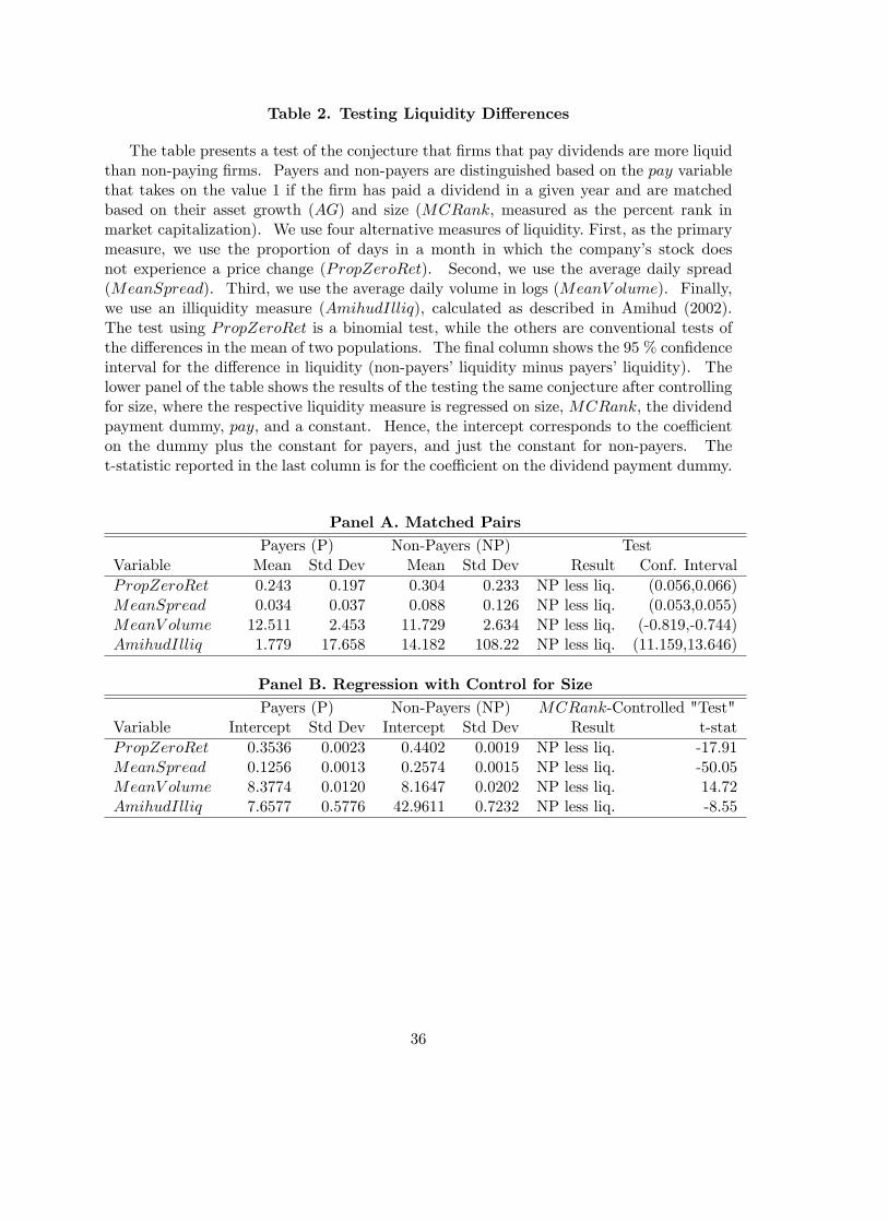
Table 2. Testing Liquidity Di¤erences

The table presents a test of the conjecture that �rms that pay dividends are more liquidthan non-paying �rms. Payers and non-payers are distinguished based on the pay variablethat takes on the value 1 if the �rm has paid a dividend in a given year and are matchedbased on their asset growth (AG) and size (MCRank, measured as the percent rank inmarket capitalization). We use four alternative measures of liquidity. First, as the primarymeasure, we use the proportion of days in a month in which the company�s stock doesnot experience a price change (PropZeroRet). Second, we use the average daily spread(MeanSpread). Third, we use the average daily volume in logs (MeanV olume). Finally,we use an illiquidity measure (AmihudIlliq), calculated as described in Amihud (2002).The test using PropZeroRet is a binomial test, while the others are conventional tests ofthe di¤erences in the mean of two populations. The �nal column shows the 95 % con�denceinterval for the di¤erence in liquidity (non-payers�liquidity minus payers�liquidity). Thelower panel of the table shows the results of the testing the same conjecture after controllingfor size, where the respective liquidity measure is regressed on size, MCRank, the dividendpayment dummy, pay, and a constant. Hence, the intercept corresponds to the coe¢ cienton the dummy plus the constant for payers, and just the constant for non-payers. Thet-statistic reported in the last column is for the coe¢ cient on the dividend payment dummy.

Panel A. Matched PairsPayers (P) Non-Payers (NP) Test

Variable Mean Std Dev Mean Std Dev Result Conf. IntervalPropZeroRet 0.243 0.197 0.304 0.233 NP less liq. (0.056,0.066)MeanSpread 0.034 0.037 0.088 0.126 NP less liq. (0.053,0.055)MeanV olume 12.511 2.453 11.729 2.634 NP less liq. (-0.819,-0.744)AmihudIlliq 1.779 17.658 14.182 108.22 NP less liq. (11.159,13.646)

Panel B. Regression with Control for SizePayers (P) Non-Payers (NP) MCRank-Controlled "Test"

Variable Intercept Std Dev Intercept Std Dev Result t-statPropZeroRet 0.3536 0.0023 0.4402 0.0019 NP less liq. -17.91MeanSpread 0.1256 0.0013 0.2574 0.0015 NP less liq. -50.05MeanV olume 8.3774 0.0120 8.1647 0.0202 NP less liq. 14.72AmihudIlliq 7.6577 0.5776 42.9611 0.7232 NP less liq. -8.55

36

Table 3. Testing Volatility Di¤erences

The table tests the implication that payers are less volatile than non-payers using threevariables: Earnings per assets (EperA), value per assets (V perA) and the �rms�stock price.Payers and non-payers are distinguished based on the pay variable that takes on the value 1if the �rm has paid a dividend in a given year and are matched based on their asset growth(AG) and size (MCRank, measured as the percent rank in market capitalization). PanelA shows the results of a test comparing the variance across two sub-samples, payers versusnon-payers, ignoring the time dimension so payers in any given year are assumed to sharethe same properties. Panel B, in contrast, compares the volatility of a typical payer tothat of a typical non-payer through time, where "typical" refers to a company characterizedby the average value of the variable of interest (EperA, V perA, or Price) at every pointin time. For robustness, we repeat the tests with the median values and obtain similarresults (results not reported for brevity). The number reported in the last column is theupper bound of a 99% con�dence interval constructed for the ratio of standard deviationof relevant variable for payers over that for non-payers. The upper bound being below 1indicates that payers are less volatile. Panel C summarizes the signi�cance of the coe¢ cienton pay in a regression where volatility over the sample period is regressed on the averagevalues of pay dummy, size, asset growth, and an industry dummy.

Panel A. Total DispersionPayers (P) Non-Payers (NP) Test

Variable Std Dev Std Dev Result BoundaryEperA 0.064 0.335 P less volatile 0.192V perA 0.966 3.042 P less volatile 0.318Price 23.644 591.57 P less volatile 0.040

Panel B. Dispersion Across TimePayers (P) Non-Payers (NP) Test

Variable Std Dev Std Dev Result BoundaryEperA 0.011 0.068 P less volatile 0.162V perA 0.250 0.566 P less volatile 0.442Price 7.308 8.249 P less volatile 0.886

Panel C. RegressionVolatility regressed on pay and controls

Variable Coe¢ cient Std Dev t-statEperA -0.099 0.001 -89.92V perA -0.854 0.010 -84.92Price -7.948 2.043 -3.89

37

Table 4. Analyzing the Relationship between Investment and AdverseSelection

The table presents the results of panel data regressions where we use PIN , a measureof adverse selection de�ned as the probability that the opening trade is information-basedand measured by the fraction of orders that arise from informed traders, as the dependentvariable and asset growth (AG) as a proxy for investment and control for earnings perassets (EperA), value per assets (V perA), size (measured by MCRank de�ned as percentrank in market capitalization), and measures of liquidity (PropZeroRet and AmihudIlliq).We also use an alternative measure of investment (Inv) as de�ned in Rajan and Zingales(1998) instead of AG for robustness. We refer the reader to Easley, Hvidkjaer and O�Hara(2002) for detailed information on the construction of PIN from transactions data. PINis available for the period between 1983 and 2001. The absolute value of robust t-statisticsare in parentheses and * means signi�cant at 10%; ** signi�cant at 5%; *** signi�cant at1%.

Panel Data Regression Results: 1983-2001Dependent variable: PIN

Speci�cation 1 2 3 4 5AG 0.015*** 0.019*** 0.015***

(7.75) (10.38) (7.84)EperA 0.015*** 0.020*** 0.017*** 0.029*** 0.026***

(4.11) (5.92) (4.78) (7.18) (6.13)V perA -0.001** 0.001** -0.001** 0.001 -0.001**

(1.97) (2.31) (2.22) (1.42) (2.22)MCRank -0.144*** -0.103*** -0.142*** -0.100*** -0.139***

(64.89) (41.90) (63.72) (29.87) (46.35)PropZeroRet 0.146*** 0.152***

(33.72) (24.53)AmihudIlliq 0.021*** 0.027***

(4.04) (3.66)Inv 0.003*** 0.002***

(4.70) (2.99)Constant 0.297*** 0.241*** 0.293*** 0.236*** 0.287***

(203.13) (109.91) (162.08) (76.92) (114.57)Observations 27,857 27,857 27,857 13,654 13,654

38

Table 5. Analyzing the Relationship between Dividend Payment and LiquidityFama-MacBeth Regressions

The table presents the results of logit regressions by year where we use the same set ofvariables as Fama and French (2001) with the exception that we add, one at a time, fouralternative measures of liquidity. The dependent variable is pay, where a �rm that paiddividends in a given year has a value of 1, a non-payer has a value of zero. AG is assetgrowth, EperA is earnings per assets, V perA is value per assets, MCRank is size mea-sured by the percent rank in market capitalization. The four alternative liquidity measuresare: the proportion of days in a month in which the company�s stock does not experiencea price change (PropZeroRet), the average daily spread over the month (MeanSpread),the average daily volume in logs over the month (MeanV olume), an illiquidity measure(AmihudIlliq) calculated as described in Amihud (2002). We present the means acrossyears of the regression intercepts and slopes, and the absolute value of t-statistics for themeans in parentheses. These statistics are de�ned as the mean of the coe¢ cient dividedby its standard error, that is, the time-series standard deviation of the regression coe¢ cientdivided by the square root of the number of years in the period, in line with Fama andMacBeth (1973). When calculating these averages, we use two di¤erent sample periods:the same as in FF (until 1998) and our whole sample. The �rst column, Speci�cation1, reproduces FF�s results for ease of comparison. Speci�cations 2-5 display our resultswith PropZeroRet, MeanSpread, MeanV olume; AmihudIlliq as proxies for liquidity, re-spectively, for the same sample period, 1963-1998. Speci�cations 6-9 present our resultsfor the extended sample period, 1963-2002. The t-statistics reported in the table are notadjusted. However, we recalculate these using Newey-West and Shanken corrections. Thenew t-statistics, although lower than the unadjusted counterparts, still indicate signi�canceat virtually the same levels. We report the unadjusted statistics in order to be comparableto FF�s results. * denotes signi�cance at 10%; ** signi�cance at 5%; *** signi�cance at1%. The R2 presented is the average of the yearly regressions�R2.

39

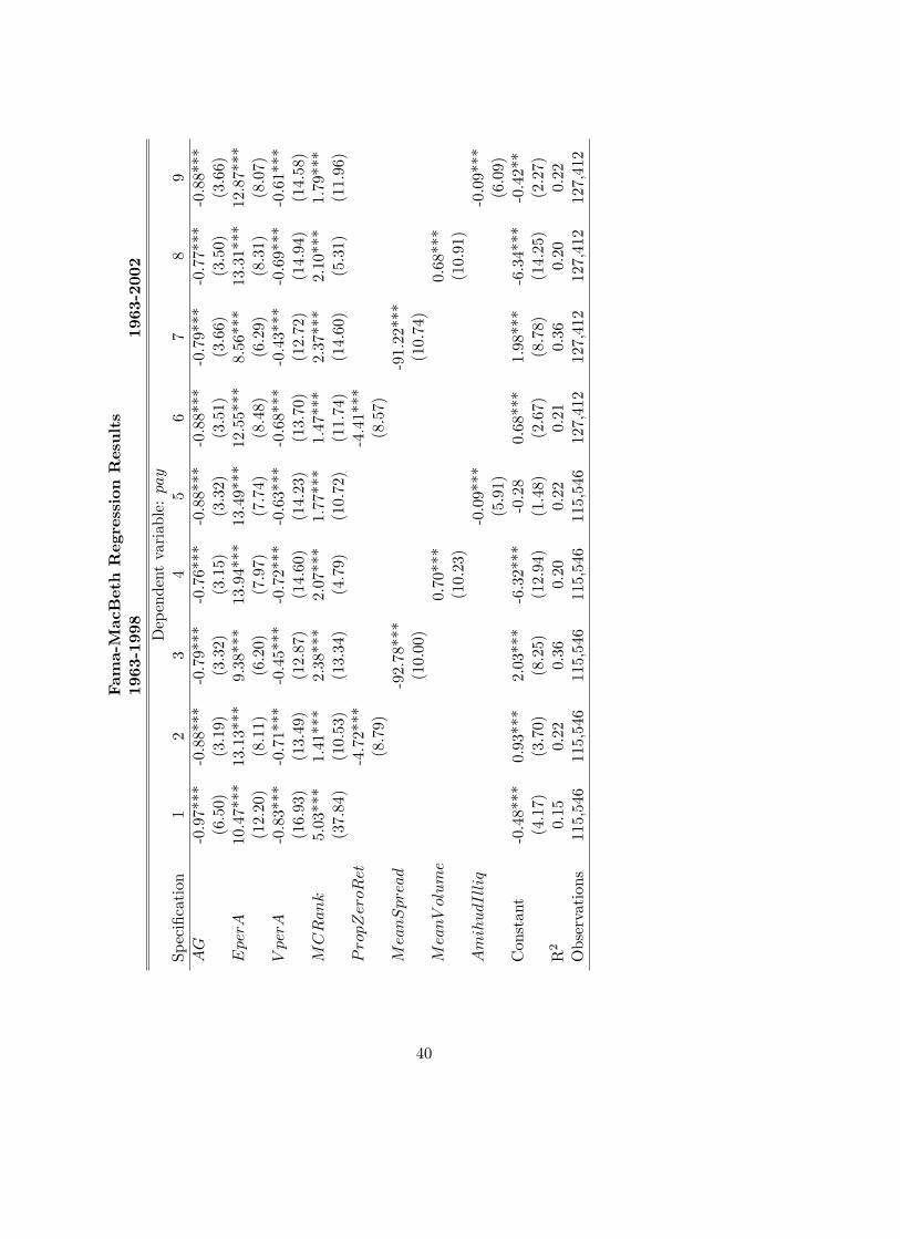
Fam

a-MacBethRegressionResults

1963-1998

1963-2002

Dependentvariable:pay

Speci�cation

12

34

56

78

9AG

-0.97***

-0.88***

-0.79***

-0.76***

-0.88***

-0.88***

-0.79***

-0.77***

-0.88***

(6.50)

(3.19)

(3.32)

(3.15)

(3.32)

(3.51)

(3.66)

(3.50)

(3.66)

EperA

10.47***

13.13***

9.38***

13.94***

13.49***

12.55***

8.56***

13.31***

12.87***

(12.20)

(8.11)

(6.20)

(7.97)

(7.74)

(8.48)

(6.29)

(8.31)

(8.07)

VperA

-0.83***

-0.71***

-0.45***

-0.72***

-0.63***

-0.68***

-0.43***

-0.69***

-0.61***

(16.93)

(13.49)

(12.87)

(14.60)

(14.23)

(13.70)

(12.72)

(14.94)

(14.58)

MCRank

5.03***

1.41***

2.38***

2.07***

1.77***

1.47***

2.37***

2.10***

1.79***

(37.84)

(10.53)

(13.34)

(4.79)

(10.72)

(11.74)

(14.60)

(5.31)

(11.96)

PropZeroRet

-4.72***

-4.41***

(8.79)

(8.57)

MeanSpread

-92.78***

-91.22***

(10.00)

(10.74)

MeanVolume

0.70***

0.68***

(10.23)

(10.91)

AmihudIlliq

-0.09***

-0.09***

(5.91)

(6.09)

Constant

-0.48***

0.93***

2.03***

-6.32***

-0.28

0.68***

1.98***

-6.34***

-0.42**

(4.17)

(3.70)

(8.25)

(12.94)

(1.48)

(2.67)

(8.78)

(14.25)

(2.27)

R2

0.15

0.22

0.36

0.20

0.22

0.21

0.36

0.20

0.22

Observations

115,546

115,546

115,546

115,546

115,546

127,412

127,412

127,412

127,412

40

Table 6. Analyzing the Relationship between Dividend Payment and LiquidityPanel Data Results

The table presents the results of panel data logit regressions for Speci�cations 6-9 inTable 5. The dependent variable is pay, where a �rm that paid dividends in a given yearhas a value of 1, a non-payer has a value of zero. AG is asset growth, EperA is earnings perassets, V perA is value per assets, MCRank is size measured by the percent rank in marketcapitalization. The four alternative liquidity measures are: the proportion of days in amonth in which the company�s stock does not experience a price change (PropZeroRet), theaverage daily spread over the month (MeanSpread), the average daily volume in logs overthe month (MeanV olume), an illiquidity measure (AmihudIlliq) calculated as describedin Amihud (2002). The absolute value of robust t-statistics are in parentheses and * meanssigni�cant at 10%; ** signi�cant at 5%; *** signi�cant at 1%.

Panel Data Regression Results: 1963-2002Dependent variable: pay

Speci�cation 1 2 3 4AG -0.18*** -0.31*** -0.15*** -0.19***

(4.33) (7.17) (3.54) (4.44)EperA 7.64*** 6.05*** 7.67*** 7.50***

(39.31) (30.84) (39.45) (39.39)V perA -0.57*** -0.50*** -0.53*** -0.54***

(29.46) (26.36) (26.77) (28.33)MCRank 2.62*** 2.48*** 3.46*** 2.97***

(21.49) (32.66) (23.72) (28.30)PropZeroRet -2.15***

(16.24)MeanSpread -42.68***

(46.93)MeanV olume -0.03*

(1.66)AmihudIlliq -0.02***

(13.96)Constant -2.41*** -1.11*** -3.17*** -3.10***

(22.46) (18.21) (21.29) (41.48)Observations 127,412 127,412 127,412 127,412

41

Table 7. Adding Shareholder PowerFama-MacBeth Regressions

The table presents the results of logit regressions by year where we use the same set ofvariables as Fama and French (2001) with the exception that we add, one at a time, fouralternative measures that proxy for the fact that shareholder power is of importance for thedecision to pay dividends. The dependent variable is pay, where a �rm that paid dividendsin a given year has a value of 1, a non-payer has a value of zero. AG is asset growth, EperAis earnings per assets, V perA is value per assets, MCRank is size measured by the percentrank in market capitalization. The four alternative liquidity measures are: the propor-tion of days in a month in which the company�s stock does not experience a price change(PropZeroRet), the average daily spread over the month (MeanSpread), the averagedaily volume in logs over the month (MeanV olume), an illiquidity measure (AmihudIlliq)calculated as described in Amihud (2002). The proxy for the impact of shareholderpower in relation with liquidity is LiqGovP (LiqGovS, LiqGovV , LiqGovA), an interac-tion variable constructed as PropZeroRet�DemDummy (MeanSpread�DemDummy,MeanV olume �DemDummy, AmihudIlliq �DemDummy), where DemDummy is 1 ifcorporate governance index, GIndex, is smaller than or equal to 5 and 0 otherwise. Thegovernance index is a variable adapted from Gompers, Ishii and Metrick (2003). It isconstructed using the incidence of 24 governance rules to proxy for the level of shareholderrights. The �rms with strongest rights are called �democracy��rms. These democracy�rms are the ones that have DemDummy = 1. The data for the governance index start in1991, hence we have to limit the sample. We use two sub-samples: 1993-1998 (to comparewith FF�s results) and 1991-2002. We present the means across years of the regressionintercepts and slopes, and the absolute value of t-statistics for the means in parentheses.These statistics are de�ned as the mean of the coe¢ cient divided by its standard error,that is, the time-series standard deviation of the regression coe¢ cient divided by the squareroot of the number of years in the period, in line with Fama and MacBeth (1973). The�rst column, Speci�cation 1, reproduces FF�s results for ease of comparison. Speci�cations2-5 display our results with PropZeroRet, MeanSpread, MeanV olume; AmihudIlliq asproxies for liquidity, respectively, for the same sample period, 1993-1998. Speci�cations 6-9present our results for the extended sample period, 1991-2002. The t-statistics reported inthe table are not adjusted. However, we recalculate these using Newey-West and Shankencorrections. The new t-statistics, although lower than the unadjusted counterparts, stillindicate signi�cance at virtually the same levels. We report the unadjusted statistics inorder to be comparable to FF�s results. * denotes signi�cance at 10%; ** signi�cance at5%; *** signi�cance at 1%. The R2 presented is the average of the yearly regressions�R2.

42

Fam

a-MacBethRegressionResults

1993-1998

1991-2002

Dependentvariable:pay

Speci�cation

12

34

56

78

9AG

-1.75***

-0.58*

-0.57*

-0.31

-0.59*

-0.69***

-0.68***

-0.53***

-0.69***

(9.95)

(1.89)

(1.91)

(1.34)

(1.87)

(3.82)

(3.78)

(3.04)

(3.79)

EperA

7.09***

5.71***

5.61***

5.48***

5.76***

6.37***

6.38***

5.71***

6.37***

(21.78)

(10.46)

(10.51)

(6.85)

(10.58)

(10.12)

(10.02)

(12.75)

(10.20)

VperA

-0.65***

-0.16***

-0.15***

-0.16**

-0.17***

-0.16***

-0.15***

-0.19***

-0.17***

(14.31)

(3.93)

(3.79)

(2.41)

(3.86)

(4.83)

(4.41)

(6.13)

(4.91)

MCRank

4.51***

1.90***

1.83***

1.67***

2.02***

1.77***

1.71***

1.40***

1.88***

(34.25)

(9.71)

(11.20)

(7.35)

(11.48)

(10.53)

(11.02)

(10.13)

(11.05)

LiqGovP

0.10

-0.44

(0.09)

(0.61)

LiqGovS

-20.86***

-24.03***

(5.04)

(8.39)

LiqGovV

0.01

0.02**

(0.34)

(2.15)

LiqGovA

-2.25**

-1.27**

(2.12)

(2.02)

Constant

-1.33***

-0.45***

-0.35***

-0.35***

-0.54***

-0.41**

-0.32***

-0.22***

-0.49***

(17.59)

(5.01)

(5.20)

(3.43)

(8.29)

(5.04)

(4.32)

(3.36)

(6.28)

R2

0.11

0.06

0.06

0.05

0.06

0.06

0.07

0.05

0.06

Observations

11,014

11,014

11,014

11,014

11,014

31,475

31,475

31,475

31,475

43

Table 8. Adding Shareholder PowerPanel Data Results

The table presents the results of panel data logit regressions for Speci�cations 6-9 inTable 5. The dependent variable is pay, where a �rm that paid dividends in a given yearhas a value of 1, a non-payer has a value of zero. AG is asset growth, EperA is earnings perassets, V perA is value per assets, MCRank is size measured by the percent rank in mar-ket capitalization. The four alternative liquidity measures are: the proportion of days in amonth in which the company�s stock does not experience a price change (PropZeroRet), theaverage daily spread over the month (MeanSpread), the average daily volume in logs overthe month (MeanV olume), an illiquidity measure (AmihudIlliq) calculated as describedin Amihud (2002). The proxy for the impact of shareholder power in relation with liq-uidity is LiqGovP (LiqGovS, LiqGovV , LiqGovA), an interaction variable constructed asPropZeroRet�DemDummy (MeanSpread�DemDummy,MeanV olume�DemDummy,AmihudIlliq � DemDummy), where DemDummy is 1 if corporate governance index,GIndex, is smaller than or equal to 5 and 0 otherwise. The governance index is a vari-able adapted from Gompers, Ishii and Metrick (2003). It is constructed using the inci-dence of 24 governance rules to proxy for the level of shareholder rights. The �rms withstrongest rights are called �democracy��rms. These democracy �rms are the ones thathave DemDummy = 1. The data for the governance index start in 1991, hence we have tolimit the sample. The absolute value of robust t-statistics are in parentheses and * meanssigni�cant at 10%; ** signi�cant at 5%; *** signi�cant at 1%.

Panel Data Regression Results: 1991-2002Dependent variable: pay

Speci�cation 1 2 3 4AG -0.32* -0.23 -0.31* -0.32**

(1.95) (1.23) (1.87) (1.98)EperA 3.13*** 4.11*** 3.26*** 3.23***

(3.66) (4.60) (3.70) (3.73)V perA -0.10 0.14** -0.07 -0.10

(1.28) (2.01) (0.78) (1.24)MCRank 5.35*** 4.99*** 5.23*** 5.11***

(10.41) (8.70) (10.63) (10.53)LiqGovP -1.05

(0.66)LiqGovS -35.40***

(5.51)LiqGovV 0.03

(1.28)LiqGovA -0.18

(1.56)Constant -3.42*** -2.87*** -3.27*** -3.19***

(7.89) (6.10) (7.95) (7.99)Observations 38,475 38,475 38,475 38,475

44

Table 9. Adding Intensity of Informed Trading

The table presents the results of logit regressions with the same independent variablesas in FF and the measures of liquidity, however, we add a new variable, PIN , to controlfor the degree of informed trading. PIN is a measure of adverse selection de�ned as theprobability that the opening trade is information-based and measured by the fraction oforders that arise from informed traders. We refer the reader to Easley, Hvidkjaer andO�Hara (2002) for detailed information on the construction of PIN from transactions data.PIN is available for the period between 1983 and 2001. The dependent variable is pay,where a �rm that paid dividends in a given year has a value of 1, a non-payer has a value ofzero. AG is asset growth, EperA is earnings per assets, V perA is value per assets,MCRankis size measured by the percent rank in market capitalization. The two alternative liquiditymeasures are: the proportion of days in a month in which the company�s stock does notexperience a price change (PropZeroRet) and the average daily spread over the month(MeanSpread). We also introdue proxies for the impact of shareholder power in relationwith liquidity: LiqGovP and LiqGovS, interaction variables constructed as PropZeroRet�DemDummy and MeanSpread � DemDummy, respectively, where DemDummy is 1 ifcorporate governance index, GIndex, is smaller than or equal to 5 and 0 otherwise. Thegovernance index is a variable adapted from Gompers, Ishii and Metrick (2003). It isconstructed using the incidence of 24 governance rules to proxy for the level of shareholderrights. The �rms with strongest rights are called �democracy��rms. These democracy�rms are the ones that have DemDummy = 1. The data for the governance index startin 1991, hence we have to limit the sample further when we use these interaction variables.Panel A displays the results from Fama-MacBeth regressions, where the means across yearsof the regression intercepts and slopes and the absolute value of t-statistics for the means(in parentheses) are summarized. These statistics are de�ned as the mean of the coe¢ cientdivided by its standard error, that is, the time-series standard deviation of the regressioncoe¢ cient divided by the square root of the number of years in the period, in line with Famaand MacBeth (1973). Speci�cations 1-3 run from 1983 to 2001, and speci�cations 4-5 runfrom 1991 to 2001. To enhance comparability to FF�s results, regressions over the period1993-1998 are shown in speci�cations 6-10. The t-statistics reported in the table are notadjusted. However, we recalculate these using Newey-West and Shanken corrections. Thenew t-statistics, although lower than the unadjusted counterparts, still indicate signi�canceat virtually the same levels. We report the unadjusted statistics in order to be comparableto FF�s results. Panel B presents the results of panel data logit regressions for the samespeci�cations as in Panel A. The absolute value of robust t-statistics are in parentheses. *denotes signi�cance at 10%; ** signi�cance at 5%; *** signi�cance at 1%.

45

PanelA.Fam

a-MacBethRegressionResults

Dependentvariable:pay

1983-2001

1991-2001

1993-1998

Speci�cation

12

34

56

78

910

AG

-0.81***

-1.03***

-0.85***

-0.57***

-0.55***

-1.16***

-1.35***

-1.08***

-0.42

-0.40*

(7.07)

(7.82)

(8.94)

(3.29)

(3.25)

(8.14)

(8.35)

(7.02)

(1.64)

(1.65)

EperA

6.68***

5.76***

3.91***

6.34***

6.36***

6.09***

5.60***

3.52***

5.59***

5.48***

(22.26)

(19.53)

(11.51)

(9.64)

(9.52)

(23.46)

(19.29)

(10.45)

(10.59)

(10.58)

VperA

-0.29***

-0.35***

-0.09**

-0.15***

-0.13***

-0.31***

-0.35***

-0.10***

-0.16***

-0.15***

(7.44)

(7.90)

(2.27)

(4.33)

(3.84)

(5.32)

(5.31)

(3.46)

(3.45)

(3.25)

MCRank

2.72***

0.68***

2.75***

0.44

0.40

2.04***

0.54**

2.10***

0.71***

0.66***

(11.22)

(4.07)

(12.19)

(1.33)

(1.28)

(10.47)

(2.09)

(15.20)

(2.76)

(2.67)

PIN

-1.06

-1.36**

-0.38

-8.21***

-7.92***

-3.40***

-3.48***

-1.78***

-8.29***

-8.12***

(1.40)

(2.11)

(0.55)

(9.05)

(9.39)

(5.82)

(5.98)

(4.62)

(14.87)

(16.08)

PropZeroRet

-6.97***

-5.62***

(15.76)

(8.72)

MeanSpread

-19.15***

-19.53***

(19.25)

(16.11)

LiqGovP

0.30

0.45

(0.36)

(0.39)

LiqGovS

-4.10***

-3.39***

(5.65)

(3.06)

Constant

-1.08***

1.80***

1.47***

1.84***

1.87***

-0.19

1.85***

1.93***

1.80***

1.85***

(4.25)

(10.80)

(5.88)

(6.83)

(7.32)

(1.12)

(8.67)

(16.33)

(12.21)

(12.01)

Observations

27,857

27,857

27,857

10,009

10,009

6,794

6,794

6,794

6,794

6,794

46

PanelB.PanelDataRegressionResults

Dependentvariable:pay

1983-2001

1991-2001

1993-1998

Speci�cation

12

34

56

78

910

AG

-0.28***

-0.28

-0.75**

-0.31*

-0.37***

-0.80***

-0.81***

-1.37***

-0.28

-0.66**

(2.96)

(1.64)

(2.26)

(1.94)

(2.73)

(2.68)

(2.88)

(4.85)

(0.65)

(2.22)

EperA

4.05***

3.47***

2.78***

3.13***

3.04***

4.07***

4.05***

3.08***

3.12**

3.71***

(11.04)

(4.00)

(7.81)

(3.65)

(3.48)

(5.16)

(4.98)

(4.51)

(2.51)

(2.80)

VperA

-0.36***

-0.07

-0.33**

-0.10

-0.03

-0.39***

-0.40***

-0.37***

-0.13

-0.14

(9.37)

(0.81)

(3.46)

(1.25)

(0.26)

(4.08)

(3.67)

(4.02)

(0.81)

(0.82)

MCRank

6.89***

5.06***

8.05***

5.50***

7.56***

6.85***

5.65***

5.32***

4.31***

2.62***

(33.93)

(9.65)

(13.76)

(10.42)

(11.01)

(14.92)

(9.12)

(10.02)

(5.13)

(2.60)

PIN

-0.03

0.99

-7.18***

1.58

-0.50

-2.73**

-2.12*

-2.37*

-2.14

-1.32

(0.07)

(0.71)

(4.60)

(1.14)

(0.32)

(2.24)

(1.91)

(1.77)

(0.91)

(0.89)

PropZeroRet

-1.58***

-2.98***

(4.42)

(3.01)

MeanSpread

-128.19***

-119.34***

(18.06)

(15.44)

LiqGovP

1.01

2.03

(0.60)

(1.58)

LiqGovS

-58.89***

-53.91**

(6.25)

(2.09)

Constant

-3.75***

-3.39***

2.51***

-3.77***

-2.43***

-4.11***

-2.84***

-1.03***

-1.36

-0.43

(19.96)

(6.29)

(4.36)

(7.14)

(4.65)

(8.98)

(4.46)

(3.65)

(1.57)

(0.65)

Observations

27,857

27,857

27,857

10,009

10,009

6,794

6,794

6,794

6,794

6,794

47

Table 10. Expected Versus Realized Proportion of PayersAn Out-of-Sample Analysis

The table presents the results of a prediction exercise. We �rst use all �rms in our samplefor each year of the 1963-77 base period to estimate logit regressions that explain whethera �rm pays dividends based on the baseline speci�cation with two alternative liquiditymeasures, MeanSpread and PropZeroRet, and obtain two di¤erent sets of coe¢ cients.We then calculate the expected percent of payers in year t by applying the average logitcoe¢ cients for the 1963-77 base period to the explanatory variables for each �rm at year t,summing over �rms, dividing by the number of �rms and multiplying by 100. Finally, wecompute the error as predicted minus the observed percentage of payers. ERR_P (_S) isthe sum of squared errors based on the regressions using PropZeroRet (MeanSpread) asthe liquidity measure and ERR_FF is the error reported by FF. We present the resultsfor two sub-samples (78-98 and 82-98) to highlight the fact that our model performs muchbetter in the 82-98 period. We also include the minimum improvement we achieve over FF(their error minus our highest error). We do not report the results using the whole sample(until 2002) to keep the results comparable to those of FF, but these are available uponrequest.

Period ERR_P ERR_S ERR_FF Minimum Improvement1978-98 4868.73 5406.70 5656.42 249.721982-98 2884.57 3016.15 5592.46 2576.31

48