linking physics with physiology in tms: a sphere field...

NeuroImage 17, 1117–1130 (2002)doi:10.1006/nimg.2002.1282

Linking Physics with Physiology in TMS: A Sphere Field Modelto Determine the Cortical Stimulation Site in TMS

Axel Thielscher*,1 and Thomas Kammer†

*Department of Psychiatry III, University of Ulm, Ulm, Germany and †Department of Neurobiology,Max-Planck-Institute for Biological Cybernetics, Tubingen, Germany

A fundamental problem of transcranial magneticstimulation (TMS) is determining the site and size ofthe stimulated cortical area. In the motor system,the most common procedure for this is motor map-ping. The obtained two-dimensional distribution ofcoil positions with associated muscle responses isused to calculate a center of gravity on the skull.However, even in motor mapping the exact stimula-tion site on the cortex is not known and only roughestimates of its size are possible. We report a newmethod which combines physiological measure-ments with a physical model used to predict theelectric field induced by the TMS coil. In four sub-jects motor responses in a small hand muscle weremapped with 9–13 stimulation sites at the head per-pendicular to the central sulcus in order to keep theinduced current direction constant in a given corti-cal region of interest. Input–output functions fromthese head locations were used to determine stimu-lator intensities that elicit half-maximal muscle re-sponses. Based on these stimulator intensities thefield distribution on the individual cortical surfacewas calculated as rendered from anatomical MRdata. The region on the cortical surface in which thedifferent stimulation sites produced the same elec-tric field strength (minimal variance, 4.2 � 0.8%.)was determined as the most likely stimulation siteon the cortex. In all subjects, it was located at thelateral part of the hand knob in the motor cortex.Comparisons of model calculations with the solu-tions obtained in this manner reveal that thestimulated cortex area innervating the target mus-cle is substantially smaller than the size of the elec-tric field induced by the coil. Our results help toresolve fundamental questions raised by motormapping studies as well as motor thresholdmeasurements. © 2002 Elsevier Science (USA)

1 To whom correspondence and reprint requests should be ad-dressed at Abteilung Psychiatrie III, Universitat Ulm, Leimgruben-weg 12-14, D- 89075 Ulm, Germany. Fax: �49 731 50026751. E-mail:

1117

Key Words: electromagnetic fields; motor cortex; mo-tor mapping; sphere model; transcranial magneticstimulation.

INTRODUCTION

Transcranial magnetic stimulation (TMS) is a widelyused research tool in the neurosciences (Hallett, 2000;Walsh and Cowey, 2000). In conjunction with stereo-tactic coil positioning devices, it allows us to stimulatecortical sites on an individual anatomical basis (Kringset al., 1997; Herwig et al., 2001; Kammer et al., 2001).However, the exact size and site of the stimulatedneural tissue is not known, even in stereotacticallynavigated TMS. A common procedure for determininga stimulation site is systematic mapping of muscleresponses as a function of the coil position over theprimary motor cortex (motor mapping) (Wassermannet al., 1992; Wilson et al., 1993). The two-dimensionalmap showing the strength of the muscle responses ateach coil position is used to calculate a center of gravity(COG) on the skull. That site on the cortex that isclosest to the COG on the skull is commonly referred toas the probable cortical representation of the targetmuscle. However, the extension of the cortical repre-sentation cannot be assessed by motor mapping (Clas-sen et al., 1998). Furthermore, motor maps often showseveral local maxima contributing to the position of theCOG. In these cases it remains unclear whether thelocal maxima result simply from noise or from severaldistinct representations. In general, inferring a corticaltarget site from the motor map is always subject to acertain amount of uncertainty and must be regardedwith caution. Correlation studies comparing the COGsof maps obtained by TMS and functional imagingmethods support this view (Wassermann et al., 1996;Bastings et al., 1998; Rossini et al., 1998; Terao et al.,1998). They consistently report a deviation of the

Received A

[email protected].

l 10, 2002

COGs in a range of 10–20 mm.

pri

1053-8119/02 $35.00© 2002 Elsevier Science (USA)

All rights reserved.

The motor maps described so far are restricted topurely physiological measurements. They do not takeinto account the physical field distribution of the stim-

ulation coil. Whereas the magnetic field is easy to cal-culate by means of the Biot–Savart law, the inducedelectric field causing neural stimulation is much more

FIG. 1. (a) Electrical field strength calculated on a plane 1 cm above the coil plane. The field strength is coded as both color and height.The inset depicts the bell-shaped form of the field strength along the axis parallel to the coil handle. (b) The 2D plot of the electrical field onthe same plane. The strength is color coded. The arrows indicate the direction of the induced currents. For the same current direction to bemaintained over various target sites, theses sites have to lie on the indicated line.

FIG. 2. Distribution of the electric field on an individual cortical surface, as rendered from anatomical MR data. The field distributionis calculated on the basis of the sphere head model for the indicated coil position, normalized to the maximal field strength reached on thecortical surface and coded as color. Notice the rapid decrease in field strength in the sulci.

1118 THIELSCHER AND KAMMER

difficult to characterize. It depends on the complexconductivity profile of the head. The currently avail-able models assume the head to be a perfect sphere inorder to reduce complexity, thereby rendering a math-ematical solution of the electric field distribution fea-sible (Sarvas, 1987; Roth et al., 1991; Eaton, 1992;Ravazzani et al., 1996). Within a purely physicalframework, such sphere models have been used to com-pare the induced electric fields of different TMS coilgeometries (Fig. 1). However, a direct link betweenpredicted fields and individual physiological data isdifficult to establish. In principle, the sphere modelscan be used to calculate the electric field distributionon an individual cortical surface. Unfortunately, thesedistributions do not provide any information about thesite and size of the stimulated cortex. For example, atthe coil position depicted in Fig. 2, a motor responsecan be evoked with high stimulator output intensity.Nevertheless, the maximum of the induced field re-sides within the prefrontal cortex and not within theprimary motor cortex.

In this paper, we present a method linking physio-logical measurements with physical models. Applied tothe motor system, it allows us to directly calculate thecortical stimulation site as well as the individual cor-tical stimulation threshold.

Our strategy is based upon three assumptions: (i)Cortical tissue is stimulated when a certain thresholdof field strength is reached. (ii) The physiological effect(e.g., the motor response) originates from a single,small cortical target area. (iii) Sphere models describethe real electric field induced in the head with suffi-cient accuracy. For the motor system, the first twoassumptions have been shown to be plausible. Thevalidity of the third assumption can be derived fromMEG studies.

(i) The relevant parameter determining the excita-tion of cortical tissue is thought to be the inducedelectric field strength (Amassian et al., 1992; Ilmoni-emi et al., 1999). Additionally, thresholds have beenreproducibly determined (Kammer et al., 2001; Stew-art et al., 2001). Taken together, this suggests thatcortical tissue is excited by TMS only if the inducedfield strength exceeds a certain threshold. This is pos-sible only if the direction of the induced electric field iskept constant, since stimulation of the motor cortexwith different current directions results in differentresponses (Brasil-Neto et al., 1992; Mills et al., 1992;Pascual-Leone et al., 1994; Kammer et al., 2001).

(ii) In the precentral gyrus, M1, the cortical repre-sentation of different muscles is known to be organizedin a somatotopic manner (Penfield and Rasmussen,1950). Although recent data suggest that a huge over-lap between representations of different muscles ex-ists, the neuronal representations for a given muscleare distributed rather narrowly (e.g., thenar represen-

tation � 5 � 4 mm, Schieber, 2001). Given the macro-scopic resolution of TMS, this can still be considered adot-shaped representation. This view is supported by aTMS study investigating input–output functions atdifferent coil positions over the motor cortex (Thick-broom et al., 1998). By and large, all input–outputfunctions of motor responses have a similar shape andsteepness, independent of the actual stimulation site.They are merely shifted by a certain value of stimula-tion intensity which increases monotonically with thedistance from the optimal stimulation site.

(iii) In magnetoencephalography (MEG), spheremodels have been compared with more complex finite-element models of the head. It could be shown thatsphere models accurately account for the magneticfield distribution of a given dipole, with the exception ofdeep frontal and frontoparietal areas (Hamalainen andSarvas, 1989). As the reciprocity theorem holds forMEG and TMS, these results can be adopted for TMS(Ravazzani et al., 1996).

In combination, the three assumptions allow to di-rectly determine the cortical stimulation site using thestrategy depicted in the following.

Think of an electrode being placed in the corticaltarget area representing the target muscle. At severalcoil positions, TMS output intensity is adjusted to in-duce a motor response of a certain constant strength.Given the assumptions (i) and (ii), the electrode willalways record the same electric field strength, regard-less of the coil position. In contrast, the electrode willrecord field strengths varying with coil position when itis displaced from the target area. Therefore, the corti-cal target area is the only position on the cortex wherethe same electric field strength is always induced for aconstant motor response, regardless of the stimulationsite.

Using the TMS output intensities derived by thismethod, the sphere model (assumption (iii)) can beused to calculate the electric field strength on the cor-tex without implanting an electrode (Fig. 2). The cor-tical target site is then identified as that positionwhere the calculated field strength is identical for allcoil positions. In the real experiment, the determinedTMS output intensities are influenced by noise. In thiscase, the target area is the cortical position at whichthe field strengths over all coil positions are most sim-ilar to each other. Mathematically speaking, this is thepoint at which the variance of the field strengths overall stimulation sites is minimal.

Assumption (i) holds only if current directions arekept as constant as possible in the cortical target area.This can be achieved by placing the stimulation siteson a line running approximately over this area, withthe coil handle kept parallel to that line. Under suchconditions, the target area “resides” on the field distri-bution curve at the sagittal section, as shown in the

1119LINKING PHYSICS WITH PHYSIOLOGY IN TMS

inset of Fig. 1a. In addition, it can be seen from Fig. 1bthat current direction is kept constant in two dimen-sions under such stimulation conditions. As the spher-ical boundary of the head suppresses radial compo-nents of the electric field this also applies to the thirddimension (Sarvas, 1987).

The general idea of the experiment is depicted in Fig.3, showing stimulator output intensities for three stim-ulation sites along the line running over the targetarea (Fig. 3a). These intensities can be used to calcu-late electric field distributions by means of the spheremodel (Fig. 3b). The field distribution curves intersectat exactly one point which coincides with the corticalrepresentation of the target muscle.

In the actual experiment, compound muscle actionpotential (CMAP) amplitudes over the whole range ofstimulator output intensities (input–output function,Devanne et al., 1997; Thickbroom et al., 1998) weremeasured at several coil positions along the line overthe target area. We recorded CMAP amplitudes in theright abductor pollicis brevis muscle (APB). Its corticalrepresentation in the precentral sulcus (Levy et al.,1991; Wassermann et al., 1996; Krings et al., 1997;Classen et al., 1998) constitutes the target area in theexperiment. The approximate position was determinedby searching for the “hot spot” with the maximalCMAP amplitude response (Classen et al., 1998). Theline on which the measurements were performed wasoriented perpendicular to the main axis of the centralsulcus, as individually determined for each subject bymeans of online tracking and visualization of coil posi-tions in the individual anatomical magnetic resonanceimages (MRI) (Kammer et al., 2001). The distributionof the electric field strength on the cortex was calcu-lated for each coil position using the half-maximal re-sponse strength measured by means of the input–out-put function (cf. Fig. 2). The cortical site wasdetermined as the voxels with minimal variance of fieldstrengths over all coil positions.

While the three assumptions are plausible, they dif-fer in their empirical support. As all the three assump-tions must be met to obtain significant results with theproposed strategy, they act as hypotheses that aredirectly tested by our approach.

METHODS

Participants

Four subjects (age 25–38 years, three male, one fe-male) were investigated. They were all in good healthand had no history of neurological disorders. The ex-periments were approved by the local internal reviewboard of the Medical Faculty, University of Tubingen,and written informed consent was obtained. All sub-jects were right-handed as assessed by the Edinburghinventory (Oldfield, 1971).

MR Imaging

High-resolution MR scans were obtained with a1.5-T Magnetom (Siemens, Erlangen, Germany) usinga T1-weighted flash sequence. For each subject, thesurface of the head was reconstructed by means ofBrain Voyager 4.4 (Brain Innovation B.V., Maastricht,The Netherlands). Additionally, the border betweenthe gray and white matter of the left hemisphere wassegmented and rendered.

Experimental Setup

Stimulation was performed with a Magstim 200stimulator (Whitland, Dyfed, UK) and a standard fig-ure-of-eight coil. The coil was held tangentially to theskull and the coil handle was oriented perpendicular tothe central sulcus using the online visualization func-tion of the positioning device.

CMAP was recorded from the right abductor pollicisbrevis muscle and peak-to-peak amplitude was as-sessed. Subjects were given auditory and visual feed-back to ensure constant low-level contraction of thetarget muscle (mean CMAP about 100 �V) (Hess et al.,1987).

The position of the coil relative to the subject’s headwas monitored online by a positioning device based ontwo mechanical digitizing arms (Kammer et al., 2001).The coil position in 6 df was stored at each TMS stim-ulus together with the CMAP amplitude.

Determination of the Line of Measurement

Prior to the experiment, the position and orientationof the line of measurement were determined. First,using a suprathreshold TMS pulse the rough positionof the maximal CMAP response (“hot spot”) was deter-mined and the active motor threshold was measured.Second, the coil was shifted laterally and mediallyparallel to the central sulcus in steps of 1 cm, in orderto specify the position of the hot spot more precisely. Ateach position, four stimuli were applied with an inten-sity of 120% of the motor threshold. The mean value ofthe recorded CMAP was calculated. This resulted in aninverted U-shaped curve of mean CMAP values alongthe central sulcus. The line of measurement was deter-mined to be perpendicular to the central sulcus and tolead through the maximum of the inverted U. In allsubjects, this line also crossed the lateral part of thehand knob.

Measurement of the Input–Output Functions andSigmoidal Fit

The coil was moved in steps of approximately 1 cmalong the line perpendicular to the central sulcus. Thiswas repeated until anterior or posterior positions werereached at which CMAP could not be obtained even at100% of stimulator output. For each coil position, stim-


uli were delivered at continuous levels of stimulatoroutput intensity starting at 20% and increasing insteps of 10% while subjects maintained a low-levelpreinnervation of the target muscle (Thickbroom et al.,1998). We chose this low-level preinnervation for tworeasons. First, compared to the relaxed state the in-put–output functions are shifted to lower stimulatoroutput intensities (Devanne et al., 1997). This made itpossible to obtain responses from a larger range of coilpositions. And second, a good reproducibility of theinput–output function has been demonstrated withlow-level preinnervation (Devanne et al., 1997). Thestimulation frequency was restricted to a maximum of0.2 Hz. Four stimuli were applied at each level and amean CMAP amplitude was calculated. The measure-ment was terminated when the CMAP amplitude hadsaturated or when 100% of stimulator output had beenreached.

Sigmoidal curves were fitted to the input–outputfunctions using the Boltzmann equation

y �A1 � A2

1 � e �x�x0�/dx� A2 ,

with A1 and A2 as the lower and upper boundaries, x0

as the half-maximal value, and (A2 � A1)/4dx as theslope at x0. Since the gradient of the sigmoidal functionis maximal at x0 and therefore the estimation is mostaccurate, the stimulator output intensities for half-maximal CMAP values were used for the calculation ofthe electric field.

A constant value of the upper boundary A2 was usedto ensure a realistic shape of the sigmoidal functions atanterior and posterior positions at which the CMAPamplitude did not saturate even at 100% of stimulatoroutput intensity. The mean value of all CMAP ampli-tudes which reached at least 90% of the maximalCMAP amplitude was calculated and used as A2.

Calculation of the Variance of Electric Field Strength

The sphere dipole model (Ravazzani et al., 1996) wasimplemented in MATLAB 6.0 (The Mathworks Inc.,Natick, MA). The dipole model of the coil was createdusing X-ray pictures and the approach explained in thesame paper. A detailed specification of the coil modelcan be found in Appendix A. The structural MR scanand the segmented and rendered left hemisphere andthe coil positions were read using custom-made soft-ware. The sphere of the model was visualized as circleson the sagittal, coronal, and horizontal planes of thestructural MR. Within the range of the coil positions itwas manually fitted to the inner surface of the skull(Ilmoniemi et al., 1999).

We then calculated the electric field strength in eachvoxel of the rendered left hemisphere for each coil

position. More precisely, the field strength for the peakvalue of dI/dt at the start of the TMS pulse was calcu-lated. Equation 12 of Ilmoniemi et al. (1999),

dI

dt�t�0 �

�2W

�CL�

�2 � 720 J

�185 �F � 16.35 �H

� 171 � 10 6A

s,

was employed to determine the maximal value of dI/dtat a stimulator output intensity of 100% (conductanceof the coil L � 16.35 �H, capacity of the stimulator C �185 �F, maximal energy stored in the capacity W �720 J, according to the specification of the stimulator).The determined value was used to convert the stimu-lator output intensities for half-maximal CMAP re-sponses into values of dI/dt by means of the rule ofproportion.

The variance of the induced field strengths of thedifferent coil positions was calculated for each voxel.The position of the voxel with the minimal varianceand the positions of the voxels with a variance �7%were determined. The result was visualized by meansof Brain Voyager.

RESULTS

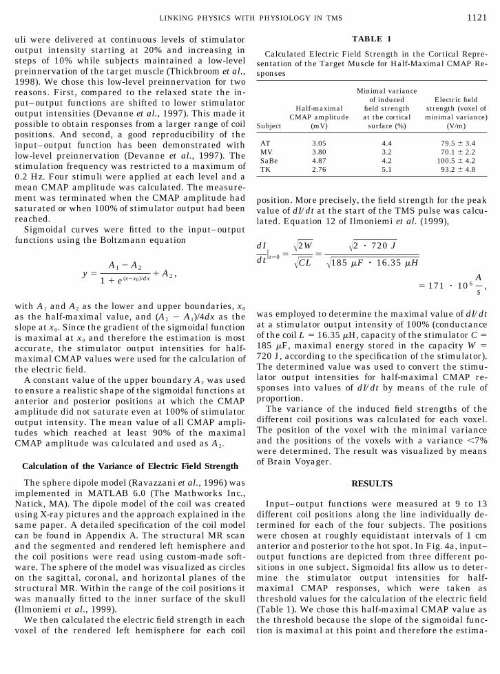
Input–output functions were measured at 9 to 13different coil positions along the line individually de-termined for each of the four subjects. The positionswere chosen at roughly equidistant intervals of 1 cmanterior and posterior to the hot spot. In Fig. 4a, input–output functions are depicted from three different po-sitions in one subject. Sigmoidal fits allow us to deter-mine the stimulator output intensities for half-maximal CMAP responses, which were taken asthreshold values for the calculation of the electric field(Table 1). We chose this half-maximal CMAP value asthe threshold because the slope of the sigmoidal func-tion is maximal at this point and therefore the estima-

TABLE 1

Calculated Electric Field Strength in the Cortical Repre-sentation of the Target Muscle for Half-Maximal CMAP Re-sponses

Subject

Half-maximalCMAP amplitude

(mV)

Minimal varianceof induced

field strengthat the cortical

surface (%)

Electric fieldstrength (voxel ofminimal variance)

(V/m)

AT 3.05 4.4 79.5 � 3.4MV 3.80 3.2 70.1 � 2.2SaBe 4.87 4.2 100.5 � 4.2TK 2.76 5.1 93.2 � 4.8


tion is most accurate. Figure 4b shows the stimulatoroutput intensities for these half-maximal CMAP re-sponses as a function of coil position. Stimulator outputintensities for the half-maximal CMAP responses of all4 subjects are shown in Fig. 5. Minor deviations froman ideal U shape occurred in three of the four subjectsat one or two coil positions.

In each subject the distribution of the electric fieldwas calculated across all the voxels in the individualcortical surface for each individual coil position used

FIG. 3. Schematic illustration of the hypothesis underlying theexperiment. (a) The minimal stimulator output intensity required toelicit a response in the target muscle is shown for three stimulationsites. The abscissa gives the coordinate of the coil position along theanterioposterior direction (y axis, 0 is arbitrarily chosen, cf. Fig. 4b),which is the main direction of coil movement at the skull. (b) Fielddistributions in the anterioposterior direction for the three coil po-sitions shown in (a). As the coil handle is orientated in the samedirection, the induced field is bell shaped (see inset of Fig. 1a). Themaxima of the fields depicted on the ordinate depend linearly on thestimulator output intensities shown in (a). Assuming that thethreshold remains constant in a circumscribed cortical region, thisregion will be stimulated at any position of the coil, but stimulusintensity has to be adjusted so that the local field strength exceedsthe threshold in this region. The target region can be calculated asthe region in which the electric field strength is the same for all coilpositions (section point of the three field distribution curves).

FIG. 4. Motor responses depend upon TMS intensities at dif-ferent stimulation sites. (a) Input–output functions for three differ-ent stimulation sites (subject AT) coded in blue, red, and purple.The half-maximal amplitudes were derived with sigmoidal fits asthe most accurate estimate of response strength to TMS. (b) Theposition-dependent TMS intensities (for half-maximal response)form a U-shaped function (middle) along the y axis of the headcoordinate system. Zero indicates the origin of the head coordinatesystem and is not related to the measured data. Notice that theordinate corresponds to the abscissa in (a). (c) The 3D model of theindividual skull as derived from the anatomical MR scan. Thespheres depict all coil positions at which input–output functionshave been measured.


(Fig. 2). Absolute values for the electric field strengthwere calculated using the stimulator output intensitiesof the half-maximal CMAPs. In each voxel of the cor-tical surface the field strength values of the differentcoil positions were compared with each other by calcu-

lating the variance. The minimal variance ranged be-tween 3.2 and 5.1% in the four subjects (Table 1), witha mean value of 4.2 � 0.8%. In Fig. 6 the voxel with theminimal variance is depicted as a red sphere on theindividual cortex for each subject. In all cases this

FIG. 5. Stimulator output intensities of the half-maximal responses as a function of the coil position. Individual data from all foursubjects are shown. On the abscissa the y coordinate of the head coordinate system is given. Zero indicates the origin of the head coordinatesystem and is not related to the measured data. The stimulator output intensities (in percentages of maximal output) are taken from thesigmoidal fits of the input–output functions measured in each subject.

FIG. 6. Area of calculated minimal variance (�7%; yellow) on four individual brains. The point of minimal variance in each case isindicated by a small red sphere. The minimal variance is given in Table 1. Light gray spheres show the coil positions used.


voxel was situated at the lateral part of the hand knob.All voxels on the cortex with a variance below 7%(arbitrarily chosen to demonstrate the distribution ofthe voxels) are indicated in yellow in Fig. 6. They forma narrow stripe perpendicular to the line of coil posi-tions crossing the hand knob. In subject TK the linewas disrupted in the junction zone of the precentraland the superior frontal sulcus.

The absolute field strength values required for half-maximal CMAP amplitudes vary from one subject tothe next, but always lie in the range of 70 to 100 V/m(Table 1).

Comparison with Model Calculations

Variance model calculations were performed in orderto account for the remaining 4.2% (cf. Appendix B). Themain results of the calculations are depicted in Fig. 7.If the remaining variance were due to systematic over-or underestimation of the field distribution or to morethan one target area, the result would be a systematicvariation of the field strength (either U shaped or in-verted U shaped) induced in the voxel of minimal vari-ance (Fig. 7a). As no such systematic variations weremeasured (Fig. 7b), the observed remaining variancecan be attributed to noise.

Finally, in a model calculation the result of the min-imal variance method assuming the maximal fieldstrength to be the relevant stimulation parameter (Fig.8a) is contrasted with a calculation considering thespatial derivative of the electric field strength as therelevant parameter (Fig. 8b). Using a U-shaped func-tion of half-maximal CMAP responses in dependenceon the coil positions (similar to the measured curvesdepicted in Fig. 5) and considering the electric fieldstrength as a relevant parameter results in a minimalvariance of 4.2% (Fig. 8a). However, the sameU-shaped function results in a minimal variance of68% when the calculation is repeated utilizing the spa-tial derivative (Fig. 8b).

DISCUSSION

Our results show that physical field models andphysiological measurements can be successfully com-bined in order to determine the cortical stimulationsite of TMS. We were able to identify, in each of thefour subjects, an area in the motor cortex where thevariance of the calculated field strengths was 5.1% orless (mean value 4.2 � 0.8%). The solutions are highlyplausible, as can be shown by data from anatomicalstudies and from model calculations.

Anatomically Correct Position of the Identified Area

The voxels with minimal variance were locatedwithin an anatomical structure that was previouslydescribed as an invariable landmark for the represen-

tation of hand muscles, the so-called hand knob(Yousry et al., 1997). Within the hand knob a somato-topic map exists, with representations of the muscles ofthe little finger located medially and representations ofthe muscles of the index finger and thumb locatedlaterally (Beisteiner et al., 2001). In all subjects thevoxel with minimal variance was located on the lateralend of the hand knob, in accordance with the knownsomatotopic map and indicating that the identified tar-get areas reside at anatomically correct positions.

Validity of the Initial Assumptions

Our results are in accordance with the three crucialassumptions of the experiment, i.e., the concept of astimulation threshold, the sufficient accuracy of thesphere model, and the dot-shaped cortical target area.However, as pointed out in the Introduction, the resultof a low minimal variance can be obtained only if allthree assumptions are met in conjunction. This is dem-onstrated quantitatively by the model calculations inAppendix B. In these simulations, the impact of viola-tions of the three assumptions on the result is exam-ined. The violation of assumption (ii), i.e., of the dot-shaped representation of a muscle, would result in asystematic deviation of the measured minimal vari-ance in dependence on the coil position (Fig. 7a). Nosuch systematic deviation was observed, but instead anoise-like distribution (Fig. 7b), thus validating as-sumption (ii). The same discrepancy between expectedsystematic deviation and measured noise validates as-sumption (iii), i.e., the accuracy of the calculated elec-tric field of the stimulation coil (Figs. 7a and 7b). Fi-nally, with regard to assumption (i), we found thealternative, i.e., the spatial derivative of the electricfield as the relevant feature determining the corticalstimulation site (instead of the electric field strengthitself), to yield 68% of minimal variance in contrast tothe obtained value of 4.2% (Fig. 8). Taken together, thesimulations reveal that the chosen experimental strat-egy does indeed react quite sensitively to even minorchanges from the initial set of assumptions. This ren-ders the production of our result by any other set ofassumptions highly unlikely, thereby validating theproposed set of assumptions.

In each subject the voxels with a variance below 7%formed a narrow stripe perpendicular to the line of coilpositions. This indicates that the resolution of ourmethod is high in the direction of the line chosen, butlower in the perpendicular direction. As the goal of ourexperiment was to test the general feasibility of theminimal variance strategy, we restricted our measure-ments to one line of coil positions. This experimentalstrategy can be augmented by measuring a second lineoriented perpendicular to the first one. By calculatingof the field variances for the two measured lines inde-pendently of each other, we should be able to find a


small intersection region of the two 7% stripes, therebynarrowing down the cortical target even further.

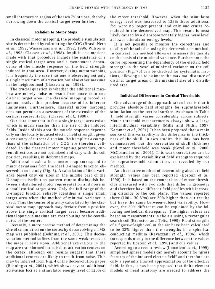
Relation to Motor Maps

In classical motor mapping, the probable stimulationsite is determined by calculating the COG (Brasil-Netoet al., 1992; Wassermann et al., 1992, 1996; Wilson etal., 1993; Classen et al., 1998). Implicit assumptionsmade with that procedure include the existence of asingle cortical target area and a monotonous depen-dence of the muscle response on the field strengthinduced in that area. However, during motormappingit is frequently the case that one is observing not onlya single maximum of activation but also other maximain the neighborhood (Classen et al., 1998).

The crucial question is whether the additional max-ima are merely noise or result from more than onedistinct target area. The classical mapping procedurecannot resolve this problem because of its inherentlimitations. Furthermore, classical motor mappingdoes not permit an assessment of the extension of thecortical representation (Classen et al., 1998).

Our data show that in fact a single target area existswhich is much smaller than the size of the inducedfields. Inside of this area the muscle response dependsonly on the locally induced electric field strength, givena constancy of current direction. Both implicit assump-tions of the calculation of a COG are therefore vali-dated. In the classical motor mapping procedure, cur-rent directions are not optimized and vary with the coilposition, resulting in deformed maps.

Additional maxima in a motor map correspond tominor deviations from the ideal U-shaped function ob-served in our study (Fig. 5). A calculation of field vari-ance based only on sites in the middle part of theU-shaped distribution pattern cannot distinguish be-tween a distributed motor representation and noise ina small cortical target area. Only the full range of theU-shaped function reliably identifies a single smalltarget area when the method of minimal variance isused. Thus the center of gravity calculated by the clas-sical motor map approach may deviate from a positionabove the single cortical target area, because addi-tional spurious maxima are contributing to the coordi-nates of the center.

Recently, a more precise method of determining thesite of stimulation on the cortex by deconvolving a TMSmap was published (Bohning et al., 2001). This decon-volution method suffers from the same weaknesses asthe maps it rests upon. Additional activations in themap are transformed into distinct activation centers onthe cortex, although our results suggest that theseadditional centers are likely to result from noise. Thismay be inferred from Fig. 4 of the deconvolution paper(Bohning et al., 2001), which shows several additionalactivation foci at a stimulator energy level of 120% of

the motor threshold. However, when the stimulatorenergy level was increased to 125% these additionalfoci were no longer present and only one center re-mained in the deconvolved map. This result is mostlikely caused by a disproportionately higher noise levelat lower stimulator energy levels.

It is not possible to monitor the correctness andquality of the solution using the deconvolution method.In contrast, our method allows us to assess the qualityon the basis of the minimal variance. Furthermore, thecurve representing the dependency of the electric fieldstrength in the voxel of minimal variance on the coilposition (Fig. 7b) can be checked for systematic frac-tions, allowing us to estimate the maximal distance ofdistinct target areas or the maximal size of a distrib-uted area.

Individual Differences in Cortical Thresholds

One advantage of the approach taken here is that itprovides absolute field strengths for suprathresholdstimulation on the cortical surface. As shown in Table1, field strength varies considerably across subjects.Motor threshold measurements always show a largeinterindividual variability (Mills and Nithi, 1997;Kammer et al., 2001). It has been proposed that a mainsource of this variability is the difference in the thick-ness of the skull. In two studies this link has beendemonstrated, but the correlation of skull thicknessand motor threshold was weak (Kozel et al., 2000;McConnell et al., 2001). This weak correlation can beexplained by the variability of field strengths requiredfor suprathreshold stimulation, as revealed by ourmethod.

An alternative method of determining absolute fieldstrength values has been reported (Epstein et al.,1990). It is based on the comparison of motor thresh-olds measured with two coils that differ in geometryand therefore have different field profiles with increas-ing distance to the coil plane. The values reportedthere (100–130 V/m) are 30% higher than our resultsbut have the same between-subject variability. How-ever, the 30% difference can be explained by the fol-lowing methodical discrepancy. The higher values arebased on measurements in the air using a rectangularsearch coil (Branston and Tofts, 1990). Field strengthsof a figure-of-eight coil in the air have been calculatedto be 32% higher than the strengths in a sphericalconducting medium (Ravazzani et al., 1996), whichcorresponds nicely to the difference between the valuesreported by Epstein et al. (1990) and our values.

According to a recent review (Ilmoniemi et al., 1999),simplified sphere models can merely account for “grossfeatures of the induced electric field” and therefore areonly a spatially limited approximation of the effectivefield. In fact, it has been proposed that finite elementmodels of head anatomy are needed to address the


complex consequences of conductance inhomogeneities(Roth et al., 1991; Liu and Ueno, 2000). In contrast tothis cautious view, we show that with respect to super-ficial cortical areas such as the motor cortex, the spheremodel is sufficiently accurate to provide quantitativeaccounts of field strength.

In conclusion, our results provide an important linkbetween the physical sphere model of electromagneticfields applied to the brain and its physiological motorresponses to TMS. Besides the implications for TMS

the validation of the sphere model supports its usewithin the context of MEG.

APPENDIX A

Dipole Model of the Magstim Figure-of-Eight Coil

A photo and two X-ray pictures of the Magstim fig-ure-of-eight coil are shown in Fig. A1. It consists of twowings with nine wire loops each. The outer and inner

FIG. 7. Electric field strength in the voxel of minimal variance as a function of the coil position, normalized to the mean field strengthover all stimulation sites. (a) Simulation results for four different systematic deviations: green, field prediction too narrow (coil size shrunkto 87%); red, field prediction too expansive (coil size stretched to 116%); blue, two distinct target areas (distance 8 mm) characterized by astep function; purple, two distinct target areas (distance 22 mm) characterized by a linear input–output function. All calculations result ina variance of 4.2% in the target voxel. Eleven stimulation sites spaced 1 cm apart on a circular line (9.5-cm radius) placed over the targetvoxel (8-cm radius) are simulated. The electric field strength in the target voxel induced by the coil position closest to it corresponds to 40%stimulator output intensity. This field strength is the threshold of the step functions and the input value for a half-maximal output of thelinear input–output functions. The two distinct target areas were placed symmetrically around the voxel of minimal variance on a circularline (8-cm radius) beneath the line of coil positions. (b) Individual data of the four subjects measured. The absence of any discernible patternin these curves indicates that noise is the main source of the variance.

FIG. 8. Comparison of electric field strength vs the spatial derivative of the induced field. (a) For all coil positions, the electric fieldstrength on a line beneath the line of coil positions and lying on the cortical surface (approximated by a hemisphere with a radius of 8 cm,origin arbitrarily chosen) is depicted (scaled to the maximum). The curves can be seen to intersect roughly in the center of the graph at 100mm. At this point, the variance is 4.2% in the model calculation. (b) The derivative of the electric field along the chosen line is calculated forall coil positions. The curves have no common intersection point. The points of minimal variance reside at 48 and 152 mm on the graph. Theminimal variance at these positions is 68%.


radii of the loops are 4.4 and 2.6 cm, respectively. Thewire is 1 mm wide and has a height of 7 mm. Thethickness of the plastic chassis is 3 mm on the sideattached to the head.

A method of approximating a coil using magneticdipoles was described by Ravazzani et al. (1996).Briefly, the coil area is divided into subregions and thedipoles are placed perpendicular to the coil area in thecenters of the subsurfaces. The dipoles are weighted bythe coil current and the areas of the subregions. Incontrast to the idealized figure-of-eight coil consistingof two loops of infinitely thin wire as modeled by Ravaz-zani et al. (1996), the Magstim coil has several loops ineach wing and a wire 7 mm high.

This was taken into account when modeling the coilas follows: The dipoles were weighted by the area of thesubregion and the amount of current circling aroundthem. A dipole in the middle of a wing is surrounded bynine loops and was therefore weighted by nine timesthe coil current. A dipole at the outer loop is sur-rounded by only one loop and consequently weighted byonce the coil current. To summarize, the length of adipole was determined by the area of the subsurfaceand n times the coil current, whereby n represents thenumber of loops surrounding the dipole.

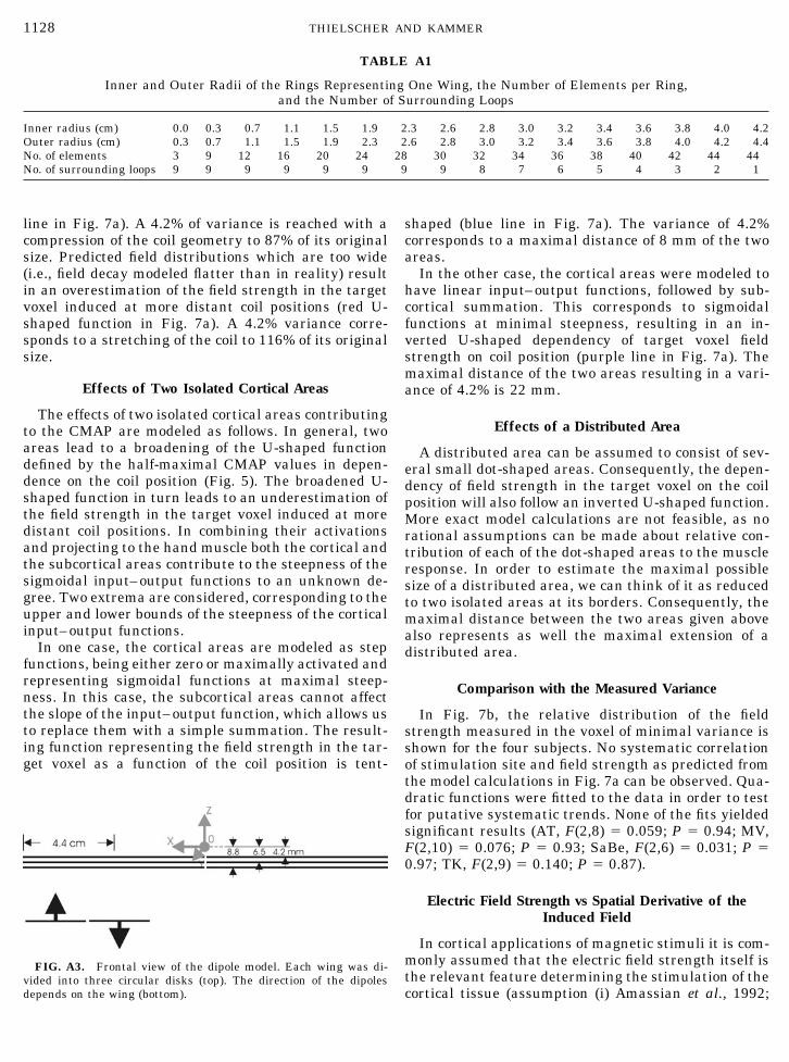
In a first step, each wing of the coil was modeled asa circular disk and divided into 16 rings. Each ring wasfurther divided into elements, as shown in Fig. A2. Theinner and outer radii of the rings, the number of ele-ments of each ring, and the number of surroundingloops can be found in Table A1.

To account for the height of the wire and the thick-ness of the plastic chassis, the circular disks were thendivided into three planes each, which were shifted 4.2,6.5, and 8.8 mm in the negative Z direction (see Fig.A3). Consequently, a plane carries one third of thecurrent and all dipoles were weighted by a factor of onethird. The current counterrotates in the two wings. Thedirection of the dipoles in one wing is therefore anti-parallel to that of the dipoles in the other wing.

APPENDIX B

We estimated the significance for the observed min-imal variance using model calculations. The minimalvariance can originate from noise, systematic devia-tions, or a combination of both. Systematic deviationsare caused by a violation of assumptions (ii) or (iii), i.e.,by the existence of a distributed cortical target area (orseveral distinct areas), or by inaccurate predictions ofthe induced electric field by the sphere model. In bothcases, the effects on the induced electric field are de-picted in the following.

Systematic Errors Caused by the Sphere Model

The effects of systematic errors of the sphere modelwere estimated for two different predicted field distri-butions which were either too narrow or too wide. Witha too-narrow field distribution (i.e., field decay modeledsteeper than in reality), the electric field strength inthe target area is progressively underestimated withincreasing distance from the stimulation sites. In thiscase, plotting the calculated electric field strength inthe voxel of minimal variance as a function of the coilposition leads to an inverted U-shaped function (green

FIG. A1. Photo and X-ray pictures of the Magstim figure-of-eight coil.

FIG. A2. Segmentation of a circular disk into elements ofrings.


line in Fig. 7a). A 4.2% of variance is reached with acompression of the coil geometry to 87% of its originalsize. Predicted field distributions which are too wide(i.e., field decay modeled flatter than in reality) resultin an overestimation of the field strength in the targetvoxel induced at more distant coil positions (red U-shaped function in Fig. 7a). A 4.2% variance corre-sponds to a stretching of the coil to 116% of its originalsize.

Effects of Two Isolated Cortical Areas

The effects of two isolated cortical areas contributingto the CMAP are modeled as follows. In general, twoareas lead to a broadening of the U-shaped functiondefined by the half-maximal CMAP values in depen-dence on the coil position (Fig. 5). The broadened U-shaped function in turn leads to an underestimation ofthe field strength in the target voxel induced at moredistant coil positions. In combining their activationsand projecting to the hand muscle both the cortical andthe subcortical areas contribute to the steepness of thesigmoidal input–output functions to an unknown de-gree. Two extrema are considered, corresponding to theupper and lower bounds of the steepness of the corticalinput–output functions.

In one case, the cortical areas are modeled as stepfunctions, being either zero or maximally activated andrepresenting sigmoidal functions at maximal steep-ness. In this case, the subcortical areas cannot affectthe slope of the input–output function, which allows usto replace them with a simple summation. The result-ing function representing the field strength in the tar-get voxel as a function of the coil position is tent-

shaped (blue line in Fig. 7a). The variance of 4.2%corresponds to a maximal distance of 8 mm of the twoareas.

In the other case, the cortical areas were modeled tohave linear input–output functions, followed by sub-cortical summation. This corresponds to sigmoidalfunctions at minimal steepness, resulting in an in-verted U-shaped dependency of target voxel fieldstrength on coil position (purple line in Fig. 7a). Themaximal distance of the two areas resulting in a vari-ance of 4.2% is 22 mm.

Effects of a Distributed Area

A distributed area can be assumed to consist of sev-eral small dot-shaped areas. Consequently, the depen-dency of field strength in the target voxel on the coilposition will also follow an inverted U-shaped function.More exact model calculations are not feasible, as norational assumptions can be made about relative con-tribution of each of the dot-shaped areas to the muscleresponse. In order to estimate the maximal possiblesize of a distributed area, we can think of it as reducedto two isolated areas at its borders. Consequently, themaximal distance between the two areas given abovealso represents as well the maximal extension of adistributed area.

Comparison with the Measured Variance

In Fig. 7b, the relative distribution of the fieldstrength measured in the voxel of minimal variance isshown for the four subjects. No systematic correlationof stimulation site and field strength as predicted fromthe model calculations in Fig. 7a can be observed. Qua-dratic functions were fitted to the data in order to testfor putative systematic trends. None of the fits yieldedsignificant results (AT, F(2,8) � 0.059; P � 0.94; MV,F(2,10) � 0.076; P � 0.93; SaBe, F(2,6) � 0.031; P �0.97; TK, F(2,9) � 0.140; P � 0.87).

Electric Field Strength vs Spatial Derivative of theInduced Field

In cortical applications of magnetic stimuli it is com-monly assumed that the electric field strength itself isthe relevant feature determining the stimulation of thecortical tissue (assumption (i) Amassian et al., 1992;

TABLE A1

Inner and Outer Radii of the Rings Representing One Wing, the Number of Elements per Ring,and the Number of Surrounding Loops

Inner radius (cm) 0.0 0.3 0.7 1.1 1.5 1.9 2.3 2.6 2.8 3.0 3.2 3.4 3.6 3.8 4.0 4.2Outer radius (cm) 0.3 0.7 1.1 1.5 1.9 2.3 2.6 2.8 3.0 3.2 3.4 3.6 3.8 4.0 4.2 4.4No. of elements 3 9 12 16 20 24 28 30 32 34 36 38 40 42 44 44No. of surrounding loops 9 9 9 9 9 9 9 9 8 7 6 5 4 3 2 1

FIG. A3. Frontal view of the dipole model. Each wing was di-vided into three circular disks (top). The direction of the dipolesdepends on the wing (bottom).


Ilmoniemi et al., 1999). Consequently, we used theexperimental strategy to search for the cortical point atwhich the variance of the field strengths over all coilpositions is minimal. In contrast, when straight pe-ripheral nerves are stimulated magnetically, nerve ex-citation is assumed to be caused by the spatial deriva-tive of the electric field (Maccabee et al., 1993).Whereas this view has been directly tested for straightperipheral nerves in physiological experiments (Mac-cabee et al., 1993), with respect to cortical stimulationno direct evidence that field strength is the relevantparameter has yet been recorded. In order to rule outthe possibility that the cortical stimulation site is de-termined by the spatial derivative of the electric field,the following model simulations were conducted.

In initial simulations, Gaussian noise was added tothe stimulator output intensities of an idealized U-shaped function for half-maximal CMAP responses un-til the minimal variance of field strength on the cortexreached 4.2% (systematic deviations were excluded asdiscussed above). Then the induced field strength wascalculated on a line beneath the line of coil positionsand lying on the cortical surface (approximated by ahemisphere with a radius of 8 cm). For all stimulationsites, the field strengths on the line on the cortex areshown in Fig. 8a. As expected, they form shifted andscaled bell-shaped curves which intersect roughly atthe point of minimal variance, here seen at 100 mm onthe chosen cortex line (compare Fig. 3).

The calculation was repeated, but the derivative ofthe electric field was calculated along the structure ofinterest, i.e., along the chosen line. For all stimulationsites, the curves generated by the derivative are de-picted in Fig. 8b. As can be seen, there is no centralintersection point. Applying the minimal variancemethod results in a minimal variance value of 68%.The points of minimal variance are shifted from 100mm (Fig. 8a) to 48 and 152 mm (Fig. 8b).

Taken together, the simulations clearly demonstratethat the use of the derivative does not allow one toidentify a cortical stimulation point. Consequently, theU-shaped functions for half-maximal CMAP responsesas measured in the experiment cannot result from cor-tical tissue sensitive to the derivative of the inducedfield, but rather stem from tissue sensitive to the elec-tric field strength itself.

ACKNOWLEDGMENTS

We thank Hans-Gunther Nusseck for technical support, as well asKuno Kirschfeld, Georg Gron, and Manfred Spitzer for fruitful dis-cussions. Michael Erb and Wolfgang Grodd provided us with theanatomical MR pictures.

REFERENCES

Amassian, V. E., Eberle, L., Maccabee, P. J., and Cracco, R. Q. 1992.Modelling magnetic coil excitation of human cerebral cortex with a

peripheral nerve immersed in a brain-shaped volume conductor:the significance of fiber bending in excitation. Electroenceph. Clin.Neurophysiol. 85: 291–301.

Bastings, E. P., Gage, H. D., Greenberg, J. P., Hammond, G., Her-nandez, L., Santago, P., Hamilton, C. A., Moody, D. M., Singh,K. D., and Ricci, P. E. 1998. Co-registration of cortical magneticstimulation and functional magnetic-resonance-imaging. Neuro-Report 9: 1941–1946.

Beisteiner, R., Windischberger, C., Lanzenberger, R., Edward, V.,Cunnington, R., Erdler, M., Gartus, A., Streibl, B., Moser, E., andDeecke, L. 2001. Finger somatotopy in human motor cortex. Neu-roimage 13: 1016–1026.

Bohning, D. E., He, L., George, M. S., and Epstein, C. M. 2001.Deconvolution of transcranial magnetic stimulation (TMS) maps.J. Neural Transm. 108: 35–52.

Branston, N. M., and Tofts, P. S. 1990. Transcranial magnetic stim-ulation. Neurology 40: 1909.

Brasil-Neto, J. P., Cohen, L. G., Panizza, M., Nilsson, J., Roth, B. J.,and Hallett, M. 1992. Optimal focal transcranial magnetic activa-tion of the human motor cortex: Effects of coil orientation, shape ofinduced current pulse, and stimulus intensity. J. Clin. Neuro-physiol. 9: 132–136.

Brasil-Neto, J. P., McShane, L. M., Fuhr, P., Hallett, M., and Cohen,L. G. 1992. Topographic mapping of the human motor cortex withmagnetic stimulation: Factors affecting accuracy and reproducibil-ity. Electroenceph. Clin. Neurophysiol. 85: 9–16.

Classen, J., Knorr, U., Werhahn, K. J., Schlaug, G., Kunesch, E.,Cohen, L. G., Seitz, R. J., and Benecke, R. 1998. Multimodal outputmapping of human central motor representation on different spa-tial scales. J. Physiol. 512: 163–179.

Devanne, H., Lavoie, B. A., and Capaday, C. 1997. Input-outputproperties and gain changes in the human corticospinal pathway.Exp. Brain. Res. 114: 329–338.

Eaton, H. 1992. Electric field induced in a spherical volume conduc-tor from arbitrary coils. Application to magnetic stimulation andMEG. Med. Biol. Eng. Comput. 30: 433–440.

Epstein, C. M., Schwartzberg, D. G., Davey, K. R., and Sudderth,D. B. 1990. Localizing the site of magnetic brain stimulation inhumans [see comments]. Neurology 40: 666–670.

Hallett, M. 2000. Transcranial magnetic stimulation and the humanbrain. Nature 406: 147–150.

Hamalainen, M. S., and Sarvas, J. 1989. Realistic conductivity ge-ometry model of the human head for interpretation of neuromag-netic data. IEEE Trans. Biomed. Eng. 36: 165–171.

Herwig, U., Padberg, F., Unger, J., Spitzer, M., and Schonfeldt-Lecuona, C. 2001. Transcranial magnetic stimulation in therapystudies: Examination of the reliability of “standard” coil position-ing by neuronavigation. Biol. Psychiatry 50: 58–61.

Hess, C. W., Mills, K. R., Murray, N. M., and Schriefer, T. N. 1987.Excitability of the human motor cortex is enhanced during REMsleep. Neurosci. Let. 82: 47–52.

Ilmoniemi, R. J., Ruohonen, J., and Karhu, J. 1999. Transcranialmagnetic stimulation—A new tool for functional imaging of thebrain. Crit. Rev. Biomed. Eng. 27: 241–284.

Kammer, T., Beck, S., Thielscher, A., Laubis-Herrmann, U., andTopka, H. 2001. Motor thresholds in humans. A transcranial mag-netic stimulation study comparing different pulseforms, currentdirections and stimulator types. Clin. Neurophysiol. 112: 250–258.

Kozel, F. A., Nahas, Z., deBrux, C., Molloy, M., Lorberbaum, J. P.,Bohning, D., Risch, S. C., and George, M. S. 2000. How coil-cortexdistance relates to age, motor threshold, and antidepressant re-sponse to repetitive transcranial magnetic stimulation. J. Neuro-psychiatry Clin. Neurosci. 12: 376–384.

Krings, T., Buchbinder, B. R., Butler, W. E., Chiappa, K. H., Jiang,H. J., Cosgrove, G. R., and Rosen, B. R. 1997. Functional magnetic-


resonance-imaging and transcranial magnetic stimulation—Com-plementary approaches in the evaluation of cortical motor func-tion. Neurology 48: 1406–1416.

Levy, W. J., Amassian, V. E., Schmid, U. D., and Jungreis, C. 1991.Mapping of motor cortex gyral sites non-invasively by transcranialmagnetic stimulation in normal subjects and patients. Electroen-ceph. Clin. Neurophysiol. Suppl. 43: 51–75.

Liu, R., and Ueno, S. 2000. Calculating the activating function ofnerve excitation in inhomogeneous volume conductor during mag-netic stimulation using the finite element method. IEEE Trans.Magn. 36: 1796–1799.

Maccabee, P. J., Amassian, V. E., Eberle, L. P., and Cracco, R. Q.1993. Magnetic coil stimulation of straight and bent amphibianand mammalian peripheral nerve in vitro: Locus of excitation.J. Physiol. 460: 201–219.

McConnell, K. A., Nahas, Z., Shastri, A., Lorberbaum, J. P., Kozel,F. A., Bohning, D. E., and George, M. S. 2001. The transcranialmagnetic stimulation motor threshold depends on the distancefrom coil to underlying cortex: A replication in healthy adultscomparing two methods of assessing the distance to cortex. Biol.Psychiatry 49: 454–459.

Mills, K. R., Boniface, S. J., and Schubert, M. 1992. Magnetic brainstimulation with a double coil: The importance of coil orientation.Electroenceph. Clin. Neurophysiol. 85: 17–21.

Mills, K. R., and Nithi, K. A. 1997. Corticomotor threshold to mag-netic stimulation—Normal values and repeatability. Muscle Nerve20: 570–576.

Oldfield, R. C. 1971. The assessment and analysis of handedness:The Edinburgh inventory. Neuropsychologia 9: 97–113.

Pascual-Leone, A., Cohen, L. G., Brasil-Neto, J. P., and Hallett, M.1994. Non-invasive differentiation of motor cortical representationof hand muscles by mapping of optimal current directions. Elec-troenceph. Clin. Neurophysiol. 93: 42–48.

Penfield, W., and Rasmussen, T. 1950. The Cerebral Cortex of Man:A Clinical Study of Localization and Function. Macmillan, NewYork.

Ravazzani, P., Ruohonen, J., Grandori, F., and Tognola, G. 1996.Magnetic stimulation of the nervous-system—Induced electric-field in unbounded, semiinfinite, spherical, and cylindrical media.Ann. Biomed. Engineer. 24: 606–616.

Rossini, P. M., Caltagirone, C., Castriotascanderberg, A., Cicinelli,P., Delgratta, C., Demartin, M., Pizzella, V., Traversa, R., andRomani, G. L. 1998. Hand motor cortical area reorganization instroke—A study with fMRI, MEG and TCS maps. NeuroReport 9:2141–2146.

Roth, B. J., Saypol, J. M., Hallett, M., and Cohen, L. G. 1991. Atheoretical calculation of the electric field induced in the cortexduring magnetic stimulation. Electroenceph. Clin. Neurophysiol.81: 47–56.

Sarvas, J. 1987. Basic mathematical and electromagnetic concepts ofthe biomagnetic inverse problem. Phys. Med. Biol. 32: 11–22.

Schieber, M. H. 2001. Constraints on somatotopic organization in theprimary motor cortex. J. Neurophysiol. 86: 2125–2143.

Stewart, L. M., Walsh, V., and Rothwell, J. C. 2001. Motor andphosphene thresholds: A transcranial magnetic stimulation corre-lation study. Neuropsychologia 39: 415–419.

Terao, Y., Ugawa, Y., Sakai, K., Miyauchi, S., Fukuda, H., Sasaki, Y.,Takino, T., Hanajima, R., Furubayashi, T., Putz, B., and Ka-nazawa, I. 1998. Localizing the site of magnetic brain-stimulationby functional MRI. Exp. Brain. Res. 121: 145–152.

Thickbroom, G. W., Sammut, R., and Mastaglia, F. L. 1998. Magneticstimulation mapping of motor cortex-factors contributing to maparea. Electroenceph. Clin. Neurophysiol. 109: 79–84.

Walsh, V., and Cowey, A. 2000. Transcranial magnetic stimulationand cognitive neuroscience. Nat. Rev. Neurosci. 1: 73–79.

Wassermann, E. M., McShane, L. M., Hallett, M., and Cohen, L. G.1992. Noninvasive mapping of muscle representations in humanmotor cortex. Electroenceph. Clin. Neurophysiol. 85: 1–8.

Wassermann, E. M., Wang, B. S., Zeffiro, T. A., Sadato, N., Pascual-leone, A., Toro, C., and Hallett, M. 1996. Locating the motor cortexon the MRI with transcranial magnetic stimulation and PET.NeuroImage 3: 1–9.

Wilson, S. A., Thickbroom, G. W., and Mastaglia, F. L. 1993. Trans-cranial magnetic stimulation mapping of the motor cortex in nor-mal subjects. The representation of two intrinsic hand muscles.J. Neurol. Sci. 118: 134–144.

Yousry, T. A., Schmid, U. D., Alkadhi, H., Schmidt, D., Peraud, A.,Buettner, A., and Winkler, P. 1997. Localization of the motor handarea to a knob on the precentral gyrus—A new landmark. Brain120: 141–157.


linking physics with physiology in tms: a sphere field...

Documents