Linking Genotypes and Phenotypes

Peter J. Park, PhD

Children’s Hospital Informatics Program Harvard Medical School

HST 950 Lecture #21

Harvard-MIT Division of Health Sciences and Technology HST.950J: Medical Computing

Introduction

•There is an increasingly large amount of gene expression data; other types of genomic data, e.g., single nucleotide polymorphisms, are accumulating rapidly.

•A large amount of phenotypic data exists as well, especially in clinical setting, e.g., diagnosis, age, gender, race, survival time, smoking history, clinical stage of tumor, size of tumor, type of tumor, treatment parameters.

•We need to find relationships between genomic and phenotypic data. What genes or variables are correlated with a particular phenotype? What should we use as predictors?

Introduction

•We need to correlate predictor variables with response variables. A classic example: is smoking related to lung cancer?

•The one of the difficulties with genomic data is that there are many possible predictors

•Eventually, we would like to have a comprehensive and coherent statistical framework for relating different types of predictors with outcome variables.

•Today: we will use micro-array data as an example.

Overview

•Microarrays have become an essential tool •cDNA arrays - basic biology labs with their own arrays (competitive hybridization – measures ratio between the sample of interest and the reference sample) •Oligonucleotide arrays (Affymetrix) – everyone else

(attempts to measure absolute abundance level) •There are few other types (SAGE, commercial arrays)

•Biological validation is necessary •northern blots; RT-PCR; RNAi

•A crude analysis may be sufficient for finding prominent features in the data, e.g., genes with very large fold ratios

•More sophisticated analysis is important for getting the most out of your data

An Observation

•There is a disconnect between statisticians/mathematicians/ computer scientists who invent techniques and biologists/ clinicians who use them.

•There have been numerous models for describing microarray data, but most of them are not used in practice.

•Biologists/clinicians are justifiably reluctant in applying method they do not understand.

•Trade-off between complexity and adoptability

Useful Techniques

Dimensionality Reduction •Principal components analysis •Singular value decomposition

Discrimination and Classification •Binary and discrete response variable •Continuous response variable •Parametric vs. nonparametric tests •Partial least squares

Censored Data •Kaplan-Meier estimator•Cox’s proportional hazards model •Generalized linear models

Statistical challenges

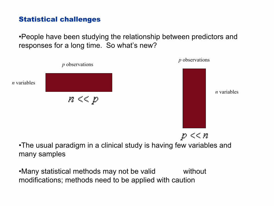
•People have been studying the relationship between predictors and responses for a long time. So what’s new?

p observations p observations

n variables

n variables

•The usual paradigm in a clinical study is having few variables and many samples

•Many statistical methods may not be valid without modifications; methods need to be applied with caution

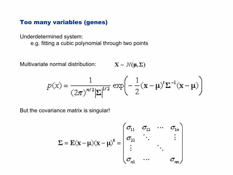
Too many variables (genes)

Underdetermined system: e.g. fitting a cubic polynomial through two points

Multivariate normal distribution:

But the covariance matrix is singular!

Statistical challenges

•One example: we need to be careful with P-values

•Suppose you flip a coin 10 times and get all heads. Is it biased? What if there are 10,000 people flipping coins

and one person gets 10 heads?

•Even if the null hypothesis is true, 500 out of 10000 genes will be significant at .05 level by chance.

•We are testing 10,000 hypotheses at the same time; need to perform “Multiple-testing adjustment”

Dimensionality Reduction

•There are too many genes in the expression data

•“Feature selection” in computer science

•Filter genes •software built-in filters •threshold value for minimum expression •variational filtering •use information from replicates

•Principal components

•Singular value decomposition

•Multi-dimensional scaling

Principal Component Analysis

We want to describe the covariance structure of a set of variables through a few linear combinations of

these variables.

Geometrically, principal components represent a new coordinate system, with axes in the directions with maximum variability.

Provides a more parsimonious description +

+

+

+ ++ +

+ +

+

+ +

+

+

+ +

+

+ +

We want maximum variance and orthogonality: eigenvectors!8

Principal Component Analysis

•Identify directions with greatest variation.

•Linear combinations are given by eigenvectors of the covariance matrix.

•Eigenvectors and eigenvalues.

•Total variation explained is related to the eigen values. Proportion of total variance due to the Kth component.

•Reduces data volumne by projecting into lower dimensions

•Can be applied to rows or columns.

Singular Value Decomposition

SVD is a matrix factorization that reveals many important properties of a matrix.

U, V are orthonormal; D is diagonal

Let ui be the ith column of U. Then the best vector that captures the column space of A is u1; the best two column vectors that capture the columns of A are u1 and u2, etc.

These vectors show the dominant underlying behavior.

In PCA, the factorization is applied to the covariance matrix rather than the data matrix itself.

Classification

•Binary classification problem using gene expression data has been studied extensively.

normal vs. cancer

genes

Typical Questions:

What genes best discriminate the two classes?

Can we divide the samples correctly into two

classes if the labels were unknown?

Can we make accurate predictions on new

samples?

Are the unknown subclasses?

Discrimination: Variable Selection by T-test

Are the means in the two populations significantly different? (two independent sample case)

normal follows a t-distribution

Requires normality! Otherwise p-values can be

misleading!

distribution

t-distribution

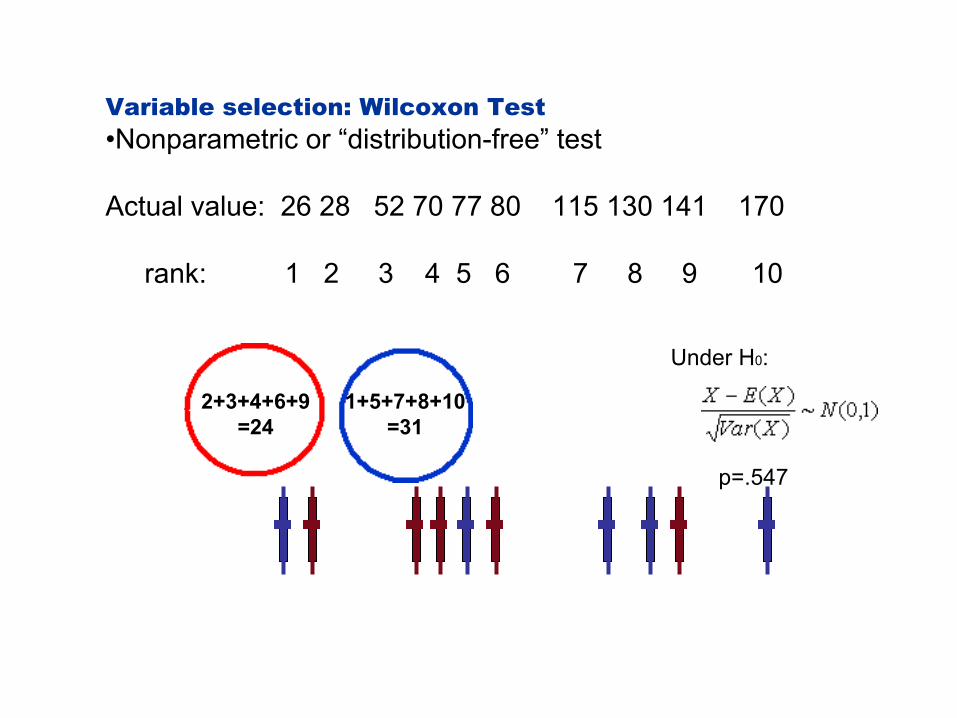
Variable selection: Wilcoxon Test •Nonparametric or “distribution-free” test

Actual value: 26 28 52 70 77 80 115 130 141 170

rank: 1 2 3 4 5 6 7 8 9 10

Under H0:

2+3+4+6+9 =24

1+5+7+8+10 =31

p=.547

An aside: hypothesis testing •The usual form of a hypothesis testing is

•For large samples, this often converges to N(0,1) under the null hypothesis.

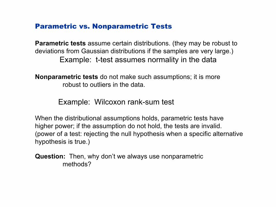
Parametric vs. Nonparametric Tests

Parametric tests assume certain distributions. (they may be robust to deviations from Gaussian distributions if the samples are very large.)

Example: t-test assumes normality in the data

Nonparametric tests do not make such assumptions; it is more robust to outliers in the data.

Example: Wilcoxon rank-sum test

When the distributional assumptions holds, parametric tests have higher power; if the assumption do not hold, the tests are invalid. (power of a test: rejecting the null hypothesis when a specific alternative hypothesis is true.)

Question: Then, why don’t we always use nonparametric methods?

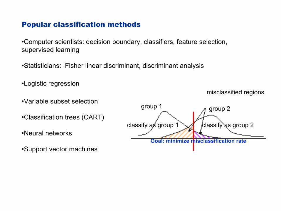
Popular classification methods

•Computer scientists: decision boundary, classifiers, feature selection, supervised learning

•Statisticians: Fisher linear discriminant, discriminant analysis

•Logistic regression

•Variable subset selection

•Classification trees (CART)

•Neural networks

•Support vector machines

misclassified regions

classify as group 1 classify as group 2

group 1 group 2

Goal: minimize misclassification rate

Multiclass classification

See Yeoh, et al. Classification, subtype discovery, and prediction of outcome in pediatric acute lymphoblastic leukemia by gene expression profiling, Cancer Cell 1(2):133-143, 2002

Classification: Remarks

•Binary classification has been studied extensively. (A popular data set: leukemia data set from Whitehead)

•Multiclass classification has received more attention recently, but more to be done. (e.g., Ramaswamy, et al. PNAS 98:15149, Bhattacharjee, et al. PNAS 98:13790)

•Use of other types of response variables has much to be done.

•Clustering (no class labels) or “unsupervised learning” has also been studied extensively. (A popular data set: yeast

experiments from Stanford)

Phenotype in many forms

•Your analysis depends on the type of phenotypic data you have.

•binary (disease vs. normal) •discrete

•non-ordered (multiple subclasses) •ordered (a rating for a severity of disease)

•continuous (measure of invasive ability of cells) •censored (patient survival time)

•Many phenotypes can be reduced to the binary type, but you lose a lot of information this way!

Using patient survival times

•Patient survival times are often censored. –a study is terminated before patients die –a patient drops out of a study –(left-censoring) a patient with a disease joins a study; we don’t know

when the disease first occurred –we assume “non-informative censoring.”

•If we exclude these patients from the study or treat them as uncensored, we obtain substantially biased results

•The phenotype can denote time to some specific event, e.g., reoccurrence of a tumor.

Previous Studies

See Alizadeh et al, Nature, 2000

Survival Analysis: Basics

•Let the failure times: T1,T2,…,Tn are iid, ~F(t)

•We are interested in estimating the survival function • S(t) = 1-F(t) = P(T>t)

•It is convenient to work with a hazard function h(t).

•h(t) is the probability of failing before t+∆t, having survived up to time t.

•h(t) = f(t)/S(t)

•We would like to estimate S(t) accurately, accounting for the censoring in the data

Survival Analysis: Parametric modeling

In a parametric model, we specify the form of S(t) or h(t). In the simplest case, we can assume that the hazard function is constant, h(t)=λ. This means F(t) follows an exponential distribution, F(t)=1-exp(-λt)

Then we can solve for the parameter λ using a likelihood approach:

We can construct likelihood functions and carry out inference

Survival Analysis: Kaplan-Meier Estimator

Data: 2,2,3+,5,5+,7,9,16,16,18+

vj Nj dj 1-dj/Nj S(t)=P(T>vj)

2 10 2 8/10 .8 5 7 1 6/7 .69 7 5 1 4/5 .55 9 4 1 3/4 .41 16 3 2 1/3 .14

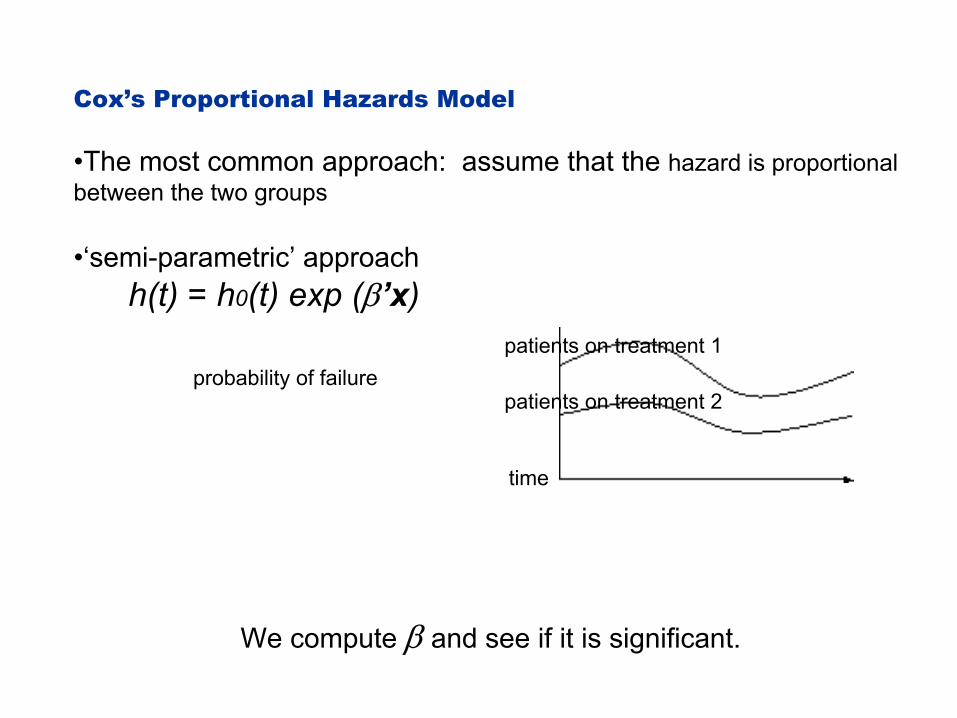
Cox’s Proportional Hazards Model

•The most common approach: assume that the hazard is proportional between the two groups

•‘semi-parametric’ approach h(t) = h0(t) exp (β’x)

probability of failure

time

patients on treatment 1

patients on treatment 2

We compute β and see if it is significant.

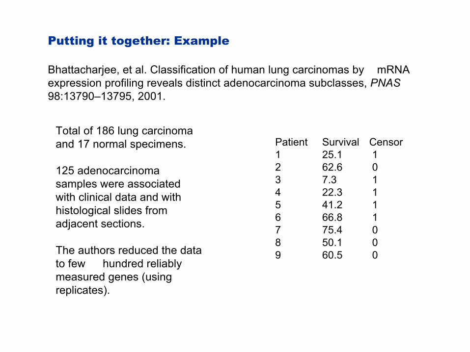
Putting it together: Example

Bhattacharjee, et al. Classification of human lung carcinomas by mRNA expression profiling reveals distinct adenocarcinoma subclasses, PNAS 98:13790–13795, 2001.

Total of 186 lung carcinoma and 17 normal specimens. Patient Survival Censor

1 25.1 1 125 adenocarcinoma 2 62.6 0 samples were associated 3 7.3 1 with clinical data and with 4 22.3 1

histological slides from 5 41.2 1 6 66.8 1adjacent sections. 7 75.4 0 8 50.1 0

The authors reduced the data 9 60.5 0to few hundred reliably measured genes (using replicates).

The Question

•Another way to deal with the censoring: turn survival times into a binary indicator, e.g., 5-year survival rate. Æ loss of information

•Question: Can we directly find genes or linear combinations of genes that are highly correlated with the survival times?

•For example, (gene A + .5 * gene B + 2 * gene C) may be highly predictive of the survival time.

•We use the survival times directly to find good predictors.

The Big Picture:

Gene expression

?

Phenotypic Data

Partial Least Squares

•Problem with dimension reduction using Principal Component Analysis: it only looks at the predictor space.

•Ordinary least squares does not consider the variability in the predictor space.

•Partial least squares is a compromise between the two. It attempts to find orthogonal linear combinations that explain the variability in the predictor space while being highly correlated with the response variable.

•Main advantage: it can handle a large number of variables (more variables than cases) and it is fast!

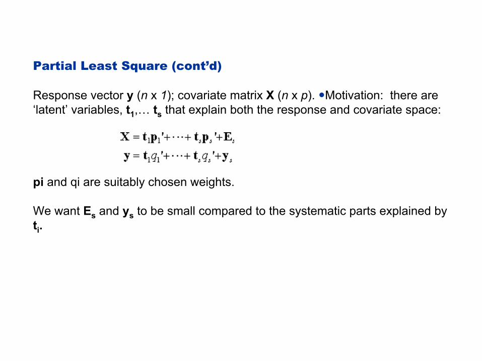
Partial Least Square (cont’d)

Response vector y (n x 1); covariate matrix X (n x p). yMotivation: there are ‘latent’ variables, t1,… ts that explain both the response and covariate space:

pi and qi are suitably chosen weights.

We want Es and ys to be small compared to the systematic parts explained by ti.

Partial Least Square (cont’d)

•Principal components analysis is based on the spectral decomposition of X’X; partial least squares is based on the decomposition of X’y, thus reflecting the covariance structure between the predictors and the response.

•Once latent variables are recovered, a regular linear regression model can be fit with latent variables.

•There are several versions of this algorithm. We use one iteratively re-weighted version.

•The algorithm is nonlinear; convergence properties are hard to understand. It is fast, as it involves no matrix decompositions.

The Big Picture: (a compromise between PCA & least squares

Gene expression Collinearity Partial Least output; ‘latent variables’)

(too many variables) Squares

?

Phenotypic Data Censoring

Reformulation as a Poisson Regression

•We would like to apply Partial Least Square to the censored problem.

•There is a way to transform the censored problem into a Poisson regression problem that has no censoring!

•We can show that the likelihood function from the new problem is the same as the one from the Cox proportional hazards model.

•Computationally more expensive, but we can do it. Partial least squares iteration is very fast (involves no matrix decompositions)

Poisson Regression

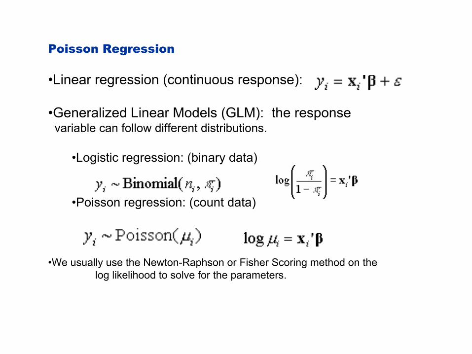
•Linear regression (continuous response):

•Generalized Linear Models (GLM): the response variable can follow different distributions.

•Logistic regression: (binary data)

•Poisson regression: (count data)

•We usually use the Newton-Raphson or Fisher Scoring method on the log likelihood to solve for the parameters.

Conclusions

•We need new methods for finding relationships between genotypic and phenotypic data

•Some basic techniques for microarray data •Dimensionality reduction •Basic classification techniques

•One example: dealing with patient survival data •Cox’s proportional hazards model •Poisson regression and generalized linear models •Partial least squares

•We need a coherent statistical framework for dealing with a large amount of various types of data