LINKAGES BETWEEN THE ECONOMY AND THEENVIRONMENT OF THE COASTAL lQNE OF MISSISSIPPI

PART I I: ENVIRONMENTAL MODEL

Prepared Under AMi s s i s s i p pi-Al abama Sea Grant

Consortium Research Grant

Edward Nissan, Ph. D.D. C. Williams, Jr., Ph.D.

Trellis Green, M.S.

Bureau of Business Research

College of Business AdministrationUniversity of Southern M~ss~ssippi

Hattiesburg, mississippi 39401

June, 1979

This work is a resu1t of research sponsored by NOAA Office of

Sea Grant, Department of Corrmerce under grant ¹04-8-MO1-92. The U.S.

Government is authorized to produce and distribute reprints for govern-

mental purposes notwithstanding any copyright notation that may appear

hereon,

HASGP � 78-041

AC KNOW LE DGEME NTS

The work upon which this report was based was financed in part

by funds provided by the Mississippi-Alabama Sea Grant Consortium. The

completion of this report is attributable to the valuable assistance

rendered by tnany individuals, busi nesses, and governmental agencies, A

special debt of gratitude is owed to Mr. Caleb Dana, Nr. carl Le Master,

Mr. Wayne Anderson and Mr. Bill Barnett of the Mississippi Air and Water

Pollution Control Corrrnission who helped in providing data, as well as

advice and guidance. Special appreciation goes to Dr. Richard Pierce of

the USM Biology Department and to consulting engineer, Mr. Lloyd Compton,

who assisted in technical and engineering aspects. Dr. Robert Nartin of

Mississippi State University proved invaluable for agricultural advice

and Mr. Leland Speed and Ms. Annette Cadwell of the State and National

Restaurant Association, respecti vely, helped overcome serious data problems .

Helpful advice concerning regional economic structure was provided by Mr.

David Veal of the Mississippi Cooperative Extension Service, Nr. Chick

Anderson of the Gulfpor t R 8 D Center, and Mr. John Howie of the Mississippi

Employment Service in Gulfport. Numerous city officials and engineers of

coastal waste treatment plants contributed beneficial field data and advice.

Graduate students Hiram Durant and Jeannie Thames contributed many man-hours

processing data. Finally, the authors are indebted to Ns, Sarah Curry who

perservered in translating the rough draft into the finished product,

Any errors of fact, logic, or judgement remai ning in the report are

the responsibility of the authors .

TABLE OF CONTENTS

AC KNOW LE DGEMENTS

LIST OF TABLES

INTRODUCTION

TYPES OF POLLUTANTS AND THEIR POTENTIAL EFFECT ON THE ENVIRONMENT.

METHODOI OGIES FOR ESTIMATING PHYSICAL QUANTITIES OF POLLUTANTSMISSISSIPPI COASTAL REGION.

Water Effluents

Air Emissions 22

Solid Waste

THE ENVIRONMENTAL MODEL � MISSISSIPPI COASTAL REGION 27

EVALUATION OF THE MODEL.

APPENDICES

45

Appendix A Estimation of Sector Outputs Mississippi CoastalRegion!.

Appendix 8 Estimation of Physical Pollutant Per Sector!.

BIBLIOGRAPHY 141

Water .Air .Solid .

Industrial Water EffluentsAgricultural Water Effluents .Comercial and Household Water Effluents

Household Category .Non-Househol d Category

Page111

1017

17

2223

48

56

LIST OF TABLES

Page

~ ~ 19

IV

IV

IV

IV

IV

Section - Table

II I 1 Percent Coverage of NAWPCC RegionalSample Industrial ClassificationSectors Mississippi Coastal Region1977.

Selected Estimated Mater ConsumptionAt Commercial Establishments NediumConcentrations.

Typical Effluent Composition of DomesticSewage Selected Values. 2O

Approximate Solid Waste Generation RatesSelected Categories......, ., 25

Average Sol id Waste Col 1 ected SelectedCategories.

Phys i ca 1 Quantities of Wate r E f f 1 uents,Air Pollution and Solid Waste MississippiCoa s ta 1 Regi on 1977......... 31

Ranking of Physical Quantities of PollutionCategory by Sector Mississippi CoastalRegion 1977 35

Quantities of Pollutants Per $10,000 OutputMississippi Coastal Region 1977 . . . . ~ 37

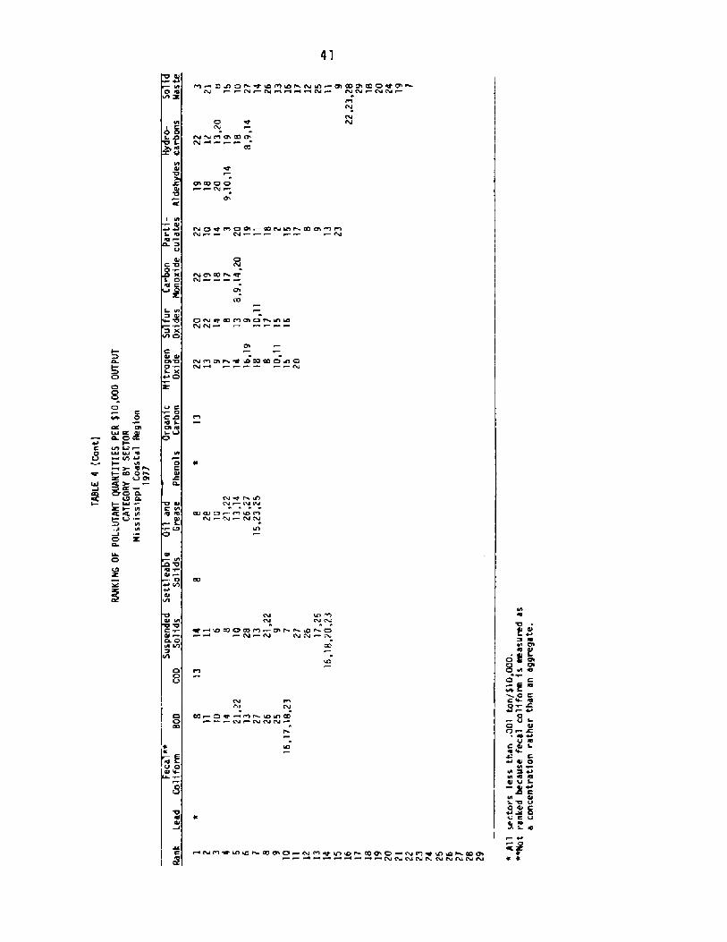
Ranking of Pollutant Quantities Per $10,000Output Category by Sector MississippiCoastal Region 1977 . . . . . . . . . . . 40

Percent of Total Pollutants Attributable tothe Top Five Sectors by Pollutant CategoryMississippi Coastal Region 1977..... 42

I . I NTRODUCTION

This report is the middle link of three projects. The earlier part

was published in March 1978 and was entitled "Linkages Between the Economy

and the Environment of the Coastal lone of Mississippi, Part I: Input-Output

Model" [38]. The study was built primarily around techniques developed by

Leontief [l8], Carter [6] and Isard [ls]. The third project will appear

subsequent to this one in a year hence,

The motivation for this three year study is to supply an empirical

investigation into the mutual impacts of economic activity and the environ-

ment in the coastal region of Mississippi. Such a study requires a consider-

able amount of data, both economic and environmental.

The economic data were furnished in the earlier report in the form of

input-output tables . There the economic activity of the region was divided

into Zg endogenous sectors, each producing output to be absorbed by the others

and in return absorbing as inputs products produced by the other sectors.

It is a fairly convenient approach to display the overall economic activity

in an accounting framework.

The non-economic data, the environmental, are by far more difficult

to obtain than the economic counterpart. In this report methods, sources

and estimates of the magnitudes of non-economic data will be presented.

In order to estimate physical quantities of pollutants in the

Mississippi coastal region, primary data published by the Mississippi Air

and Water Pollution Control Commission MAWPCC! were used when possible.

However, it was necessary in many instances to rely on secondary sources

either from similar studies or from published findings of the Environmental

Protection Agency EPA!. At times, reliance was strictly based upon esti-

mation techniques obtained from engineering and scientific publications.

The primary endeavor was to allocate physical volumes of pollutants

to the proper economic sectors as categorized by the Input-Output study f>~j.

Such allocation required a great deal of effort to systemize and analyze

diverse aggregate data. In what fol'iows a schematic outline of the methods

and procedures undertaken is discussed in detail. The analysis is focused

on the three main categories of pollutants which are:

A. plater Eff1 uents8. Air PollutionC, Solid Nastes

l'he third phase of the study whi ch is the linkage between the economyand the environment wi'l 1 follow techniques adopted by lsard [14j and manyothers in the area of regional economics.

It is necessary to ointp out that in order to conform the economicdata which are for the ey ar 1912 with the environmental data which are forthe year 1977 it was necessary to update the economic data. This was donein order to compute values of pollutants per it

r un o sales as shown inSection IV.

II. T?PES OF POLLUTANTS AND THEIR POTENT!AL EFFECTON THE ENV[RONHENT

Many different types of pollutants are discharged into the eco-

system as waste by-products of economic activity. These waste residues

are frequently wholly or partially untreated for their harmful effects.

Utimately diffused into water, air, and land, the qualitative impact upon

human and animal life, as well as non-living inputs to the economic system,

will be barn 1argely by future generations. However, recent experiences

with hazardous wastes suggest that proliferation of waste residues has

already begun to adversely affect living and non-living resources. This

section outlines the types and effects of pollutants found in water, air,

and land regions of the Nississippi Coastal Zone.

It is important to propose a useful definition of waste for this

particular study. In a study of a similar type in the state of Washington

[9], waste was defined after posing the following questions:

When is a material a waste and when is it a by-product'?It was decided that if a "waste" material from an industry'smain production process is recovered and made into some productin a plant, then this is a by-product. Also, if some materialis rejected from the process, but is returned to the process asa new material, then it also is not a waste. However, if amaterial is rejected from a firm's process and it then is shippedoff the premises f' or disposal or for use or recovery by anotherfirm, this material is deemed a waste product.

This is a broad definition of waste and is perhaps inconsistent with

the purpose of this study. It was then decided that waste be defined as the

residual disposed into the environment after being treated at a waste treat-

ment facility. That is, if part of the original waste has been treated and

deemed unharmful to the environment, it will not be considered as part ofthe waste residual inventory.

pollutants in this study can be classified i nto water effl uents,

a;r emissions, and solid waste. What follows is a brief outline and discuss~ 'of the major types encountered.

Water Pollution

Specialists in thi s area categorize water pollutants as chemical,

physical, biological and physiological. Water pollutants considered i n ttestudy are:

Benarde [3! gives a lucid description of the chemical, phys ical, biologicaland physio'iogical water pollution as follows:

The chemical pollutants include hot,h inorganic and organiccompounds, such as dai ry, textile, cannery, brewery, and paper-mi 1 1wastes, ensilage, laundry wastes, manure, and slaughterhouse wastes .These essentially contain proteins, carbohydrates, fats, oils, resinstars and soaps. If the pollutants are not excessive, they will bestabilized by the self-purification process. If they are excessive,death of fish and offensive odors can result. In addition, suchplant nutrients as phosphates, nitrates, and potassium have theability to aid weed growth and promote algae blooms which furtherdeplete oxygen. Inorganic salts, particularly toxi c heavy metalsnot removed by the standard sewage-treatment process, can producewater unsuitable for industry, i rrigati on, and drinking.

biological pollutants include the many types of microscopicani mai and plant forms, such as bacteri a, protozoa, and virusesthat are associated with disease transmissi on. These come fromdomestic sewage, farms, and tanneries.

Physiological pollution manifests itself as objectionable tastesand odors. These may be imparted to the f iesh of fish, making

'Inedible, or water itself may become unfit to drink owingt» ts odor and taste. Odors and tastes occur in water as a

Waste WaterPH Abnormal!Temperature Elevated!Ch'lorine

NitrogenSul fidesFlouridePhosphate

Heavy MetalslincCadmi umIronChromiumAluminum

CopperNickelLead

Fecal Coliform800 Abnormal!COD Abnormal!Suspended SolidsSettleable SolidsOil and GreasePhenolsOrganic Carbon

consequence of the presence of inorganic chemicals, and ashydrogen sulfide, or the extensive growth of certain speciesof algae. Some impart musty odors, while others give fishy,pigpen, spicy, or chemical tastes ta it.

Various physical effects, such as foaming, color, turbidity,and increased temperature are also considered forms of pollution.

Elevated temperature also plays a part in water pollution.Water from a nearby stream or river is pumped into a plant tocool a machine or process that normal 'ly generates heat. The transferof heat to the cooling water raises its temperature severaldegrees. When this heated water is discharged back into thestream or ri ver whence i t came, it can disrupt ecological relation-ships within it. A rise in temperature of only a few degreescan be lethal to a variety of aquatic plant and animal forms,which, like most living things, are sustained only within a narrowtemperature range. The death of certain species removes the foodsupply of species which prey on them; without this food supply theyin turn will die or be forced to move downstream. Furthermore, thewarmer the water, the less oxygen it wi'll contain; oxygen, as hasbeen pointed out, is vital for the prevention of deterioration. Atelevated temperatures all chemical and biological acti vi ty proceedsat a more rapid rate than would normally prevail, and this in turndepletes the sensitive oxygen bal ance of the stream. This seriesof events can result in the loss of self-purification capacity byaltering the stream comnunity.

Air Pollution

In this study, air pollutants considered are:

Nitrogen oxideSulfur oxidesCarbon Monoxide

ParticulatesAldehydesHydrocarbons

are small pieces of materials dischargedto the air by burning f'uel, and by industrialprocesses. When fuel is burned, small piecesof unburned material pass to the atmosphere.Large particulate discharges result from theburning of a tan of' coal or wood, whereaspetroleum products and, especially, natural

Parti cul ates:

6y wei ght, these substances account for the major discharges of

air pollution. In the United States carbon monoxide represents about half,

followed by sulfur oxides and hydrocarbons, with particulates and nitrogen

oxides representing smal'ler amounts[22!.

Mills [22] gives a descri pti on of the major ai rborne di scharges as

follows:

gas generate only small amounts ofparticulates per ton. Any coal-firedcombustion system, whether for space heatingor thermal electric generation, dischargesparticulates. Diesel engines in large trucks >buses, and some cars discharge small amountsof particulates, but internal-combustionengines discharge almost none. After dischargeto the atmosphere, particulates disperseaccording to the wind pattern. Eventual'ly,they fall to earth, mostly within a few milesof the point of discharge. Particulates varygreatly in size, which strongly effect theirdispersion, the speed with which they settleout of the atmosphere, and the harm they doto people and property.

Sulfur oxides: most sulfur in the air over urban areas resultsfrom human activities, particularly the burningof coal and oil, but also from a variety ofindustri al processes, esperially smeltingand refining. Some kinds of coal and oil containmuch more sulfur than others. All the sulfur inthe fuel at the time of combustion is releasedduring combustion and enters the atmosphere unlesscaptured beforehand. Sulfur oxidizes in theatmosphere and most washes back to earth as dilutesulfuric acid during precipitation. Heating oilused for space heating is a major source ofsulfur di scharges, as is the heavy oil used inthermal electric generation and in large space-heating uni ts in apartment houses and otherlarge buildings.

Nteoxide: virtually all the carbon monoxide in theatmosphere is discharged by human activities .Most results from burning gasoline in internal-combustion engines, but some results from manyindustriaI processes. Carbon monoxide resultsfrom incomplete combustio~ in internal-combustionengines, and less is discharged the more completethe combustion. Carbon monoxide i s an apparentlyinert gast in the atmosphere; it does not reactwith other substances there. Yet much of themassive discharge of carbon monoxide in metropoli ta~areas disappears within a few hours, at a rateapparently not explainable by the circulation ofair. lt is still something of a mystery whathappens to it.

Carbon

Hydrocarbons: they are discharged from the combustion of fossilfuels, from industrial processes, and from a variet~of miscellaneous sources. Among the later areevaporation of industrial solvents and the wearingof motor vehicle tires from driving, Like carbon

monoxide, hydrocarbons are the products ofincomplete combustion in internal-combustionengines, the largest single source of hydrocarbons .Important natural processes also discharge hydro-carbons, and in much larger quantities thanhuman activi ties on a worldwide basis. As withsulfur oxides, human activities account for mosthydrocarbons in the atmosphere over urban areas.Hydrocarbons are reactive in the atmosphere. Alongwith nitrogen oxides, they result in the formationof photochemical smog in appropriate climaticconditions.

rogen oxides: they are naturally present i n the atmosphere inlarge volumes. Most nitrogen discharges from humanactivity are converted to nitrogen dioxide, buthuman activi ty accounts for only a minor partof all atmospheric nitrogen dioxide. Virtually allnitrogen discharges from human activity result fromcombustion of fossil fuel s in motor vehicles, spaceheating systems, and thermal electric plants.Whereas carbon monoxide and hydrocarbons are theproducts of incomplete combustion, nitrogen oxides arethe natural products of' combustion. Therefore,procedures to improve the efficiency of combustionreduce carbon monoxide and hydrocarbon discharges~but increase nitrogen oxide discharges. In theatmosphere, nitrogen dioxide is an ingredient inthe formation of photochemical smog. Photochemicalreactions take place within a few hours of discharge.Nitrogen dioxide that does not take part inphotochemical reactions is removed from the atmos-phere as aerosols by settling onto the earth and byrain, mostly within three days of discharge.

Nit

Solid Waste

Pub 1 i c Works Ass oci at i on [3! classifies these as follows:

Rubbish: Includes combustible items, such as cartons,boxes, paper, grass, plastics, bedding andclothing and non-combustibles, such as ashes,cans, crockery, metal furniture, glass, andbathtubs.

Garbage: Waste resulting from growing, preparing, cooking, andservino food. Included in this category are market~astes. Together they account for approximately10 per cent of the volume of solid waste collected [z!.

Refuse: The term has been used to denote all types of waste.

Solid wastes include rubbish, refuse, garbage and others. The American

Other types of waste include demolition waste such as bricks,

masonry, pi ping, and 1 umber and sewage-treatment res i due such as septi c-tank sludge and solids from the coarse screening of domestic sewage.

For more information regarding water and air pollution and solid

the reader is referred to Bel 1 [2], Benarde [3], Dol an [10], Nil 1 s [2~] .

and lwick and Benstock [53],

METHODOLOGIES FOR ESTIMATING PHYSICAL

QUANTITiES OF POLLUTANTSMISS ISSIPP I COASTAL REGION

A. Water Effluents

Wate~ Effluent CategoriesEffluent Type and Data Sources

Mississippi Coastal Region

Source sMa or Effluent T eCate or Sector

U.S. Census ofAgriculture

MAWPCC

Ag ri cul tural

industri al

Comnerci a 1

Households

Irri gati on

Indus t ri a 1 P roces sWaste

Waste Water Sewage

6-17; 20

MAWPCC 8 Secondary18-l9; 2l-29

Waste Water Sewage MAWPCC 5 Secondary

A waste water treatment facility is classified as industrial,

municipal, or private. The industrial facilities, also called "package

Water effluent loadings were derived basically from 1977 waste

water treatment faci li ty printouts provided by the Mississippi Air and

Water Pollution Control Conmission MAWPCC! [23]. For estimation purposes

the 30 endogenous and exogenous sectors of the updated input-output model

were divided into the four categories listed below to conform with printout

classifications and effluent type. The data were the primary source for

all categories except Agriculture. To estimate household and comnercial

water wastes. the use of secondary data was necessary.

plants," process was e wat water from specitic firms which hold state permits.

Under 1977 permit stipulatiOnS, effluents prOduced by firms as conSequencesof their production processes were identified and monitored periodical lyat disc arge p '"d' h oints" to determine compliance with the standards. However,some manufacturers utilize city facilities which are neither municipalnor private and as such are not monitored, This is a particular problemfor large, privately-owned industrial parks. Thus, it was necessary toprovide estimating procedures of water effluents for such firms. Themunicipal and private facilities, on the other hand, process waste watersewage of comnercial establishments, shopping centers, apartment complexes,schools, and private households. A few monitored municipal facilities,

however, do receive wastes from manufacturing firms, usua'lly because ofgeographical proximity. Such instances required a knowledge of specificloadings by the firm since facilities rather than firms usually hold

the necessary permi ts.

Industrial plater Effluents

Factory printouts for manufacturing firms in the Mississippi coasta'l

region were classified by product into SIC categories corresponding to their

respecti ve input-output sector groupings, a sector being one or more

industries [29]. Three sectors not conventionally classified as manufacturing

--Mining, Construction, and Communi cations/Public Utilities-- were included with

manufacturing simply because they were monitored in the same fashion.

The level of information obtained from the printouts for each firm

in the coastal region was gathered as illustrated in the following to yield

net estimates of effluent wei ghts in pounds and million gallons of waste

water entering the environment after treatment. In addition, data on PH and

temperature were recorded. Monthly sample observations per discharge

point i n uni ts of wei ght pounds! or concentration milli grams per liter!

were cOnVerted tO yearly estimates, assuming a 300 day induStrial year

[39]. Sample data were published as a range from minimum to maximum with

The weights in poundsthe average reading taken where possible [8 j.

Pounds/day = MG/L x 8.34 x Flow Rate

whereNG/L = Milligrams per liter8.34 = Conversion factor

Flow Rate = Million gallons water per day

The technique followed is illustrated by the following example for a

hypothetical firm A. Assume that the BOD discharge is given in pounds and

suspended solids are recorded as 29.98 MG/L for all months at the discharge

point. Further assume that only three months are sampled for this hypothe-

ticall firm. Biological oxygen demand BOD! and flow rate waste water!

are averaged and converted to yield 33,000 pounds and 150 million gallons

per year, respectively, as follows:

3 ! lbs. x 300 days = 33,000 lbs./year100 + 110 + 120

and

.5 + .4 + .6 3 ! NGY x 300 days = 150 MGY.

To convert suspended solid concentration to pounds, Equation 1 is

applied to 29,98 NG/l and each corresponding flow rate to yield an average

of l25 pounds per day as shown in the computati ons below. The daily average

is then converted to an annual quantity of 37,500 pounds.

were obtai ned di rectly as daily averages and were then converted to an annual

basis. Neasurements that were gi ven as milli grams per liter NG/L! requi red

an indirect conversion to pounds by the following formula for a given effluent

and fi rm:

12

Suspended solids = �9.98! 8.34! .5! + �9.98! 8.34! .4!+ �9.98! 8.34! .6!

Total per day = 125 + 100 + 150 = 375Average per day = 375 ;- 3 = 125

and hence,

The total is 125 x 300 = 37,500 lbs.

Hypothetical Firm WorksheetWater Effluents

Firm A

*SU - Scientific units

1f a firm had more than one discharge point, all discharoe ooints

were sunned to give total firm loadings. Total firm outputs of water

effluents were then compiled on sector worksheets such as shown in the

fo11owing figure. For example, BQD discharges by Firm A added to all other

firms in Sector 1 total 183,000 pounds,

Hypothetical Sector WorksheetMater Effluents

Sector 1

BODFirm Em lo ment

150

100

150

Total*SU

300 183 000 170 000 300= Scientific units

50 33,000

100 60,000

150 1 00,000

Suspen eSolids lbs PH SU * Flow Rate MGY

37,500

60,000

80,000

13

E kA

eMk

�!

where:E = Effluent estimation based on allowable

permit conditionsA< = Actual reported effluent value of known fi rmsM~k = Maximum allowable permit value of known firmsM = Maximum permit value of unknown firm

Some firms contained extensive effluent concentrations MG/L! but

no flow rate to convert to pounds. In such instances an average f low rate

per employee was developed from similar firms in the sector and applied

For manufacturing firms which dump their wastes into monitored

municipal facilities rather than their own it was necessary to identify and

allocate their proper effluent loadings from the total commercial and

household wastes of the facility. The resulting effluent quantities were

then entered on manufacturing worksheets and processed as if monitored

separately. Facility worksheets then consisted of purely non-manufacturing

wastes, that is, commercial and household. This procedure was particularly

essential in the Food Processing sector, requiring primary data collected

in the field.

Many data problems were encountered when processing the printouts,

often necessitating less than optimal solutions. Missing or incomplete

data were handled in a variety of ways. For example, many fi rms wi th a

permit printout had no effluent sample results but did list maximum allowable

permi t conditions . Unpublished data provided by the MANPCC and regional

research and development center often determined whether to base estimation

of the unknown fi rm's pollution upon allowable permi t ranges or to omi t the

firm and estimate later. Estimations based upon per~it conditions were

generated with Equation 2. Maximum conditions were used because few average

permit condi tions were listed.

average annual employment. Some firms not listed in the manu-to known aver

facturer 's directory were monitored. These firms were processed ifemployment data and SIC products were available. The inclusion of thesefirms tended to balance out those listed firms which were not monitored.

After the data in all sectors were processed, a measure of the

adequacy of the regional samples was undertaken as shown in Table 1.The percent of total firms and total employment covered in earh manu-

facturing sector suggested that data supplementation was needed. Although76 percent of employment was covered, one particular firm in the Transpor-tation Equipment Sector accounted for over 6O percent of total regional

manufacturing employment. Omitting this one fi rm resulted in only 16

percent of employment being covered.

On a sector-by-sector basis half had less than SO percent coverage

and three had no coverage. Thus, two types of supplementation were needed;

sector and product. Sector supplementation was requi red for extremely low

coverage of all products such as the Apparel sector. Product supplementation

sought to give coverage to specifi c categories of products produced i n the

region but not by firms in the regional sample, for example, Food Processing.

The idea is to simulate the unaccounted region with data of similar

firms producing similar products in other parts of Mississippi and monitored

with a co+non sampling procedure. In using the non-regional supplementary

data, the assumption is made that simi lar fi rms have similar patterns of

waste loadings [25].

To select the supplementary data, lists of all Mississippi coastal

« ~ in each sector and their respecti ve SIC products were compared to

the firmse firms and products of the regional sample. Using firm employment and

product coverage, the degree of supplementation was ascertai ned. For

exa le thmp e, the Apparel sector required total sector supplementatio n. The Food

QIQr rdu tt- 5-

0 QIQIG. 0

0 KQJ

Urt EQICt. '0

0

O P4

Qp

c E

I0~r

0UJ r

0 0IQI

C trt QIQP

EQP tt- rdD

DI LA

0 WO Ch

CL

I

0r0I tilQ!CY Irrg

0

Erd

r

E S- 0'I r

QI tlat

QpC QI

S0 QIo EQJV! Z

hJ & 'Cf LO

E 0rd4-

rd

0

0

O

O QI0 OCLI trtVlr

td~ r 0

cI: Er QICL O

OIL

tP

PS

0 00LI CK

C D0

0> QI

0 0

~ W

C Vrd trtI � K

DII5-

0rd

CJDO0 ~Z r

IQI

M IQ

'U

C4CV N c0 OQIt/l rdQ OD

cC m

cZ OK LNDNUKM DCY r � r

I�O cCU O

t/!U D M

Ltt M

D cnD

I � Z

4 O A DQ ~DP!BD 4CTI 'Q M CJI

P!AXNRP!CVrP!O'rdLA< Vt&IWCVNAP!Ol~~wAA<Ow%OOAA ~ 92CV~ ~ VJ WY!r u3

AJ

r OCh40<D~DD>Wt0IDO OcQsf ADr * A

C4 ttJ

w O cq O P D 0 Ch e D 0LA VJ O

A&Mr ~NP!P!OI<~P! Q

OQ Qr ONNW D+CV

tttttI Cttrd r-r rdCg M

rdO td

~ ' I

0 rL

tA CL

processing sector, though wi th over SO percent coverage in the regi onalcontained effluent data only from seafood processors. In order to

give ai ve a more accurate sector prof i 1 e, f i rms wi th catego ri es such as beverages

and bread were needed. Thus, bottlers and bakeries in other areas of

Nississippi were added to the regional sample as supplementary data. The

regional research and development office and engineering experts as well asthe manufacturer's directory were instrumental in selecting non-regional

firms to include in the supplementary sample.

Selected non-regional firms were then processed on worksheets in

the same manner as regional firms. Total sector poundage of water effluents

was estimated by adjusting the regional quanti ties to correspond to total

area employment, utilizing both regional and selected non-regional data

when necessary. The computational procedure sumnarized in Equation 3

implies a proportion of the mean taken from the regional and non-regional

samples for the supplementary data. Average effluent per employee X of

the supplementary sample was weighted by the factor correspondingnl +n

n7to regional sample employment and a factor corresponding to non-nl + n7

regional sample employment.n] n7

�! Xl i + ] 1 X7inl + n7

nlX + Xnl + n7 I nl + n7

where

X = Average effluent/employee, supplemental sample lbs/emP!nl= Regional sample employmentn7= Non-regional sample employmentXl= Regional effluent/employee, supplemental sample Ibs/yr!>7= Non-regional effluent/employee, supplemental sample

lbs/yr!

industrial sector water pollution X was computed as shown in

E uationquat~on 4. Estimated tonnage of the uncovered sector is equal to NX. Thus,

the actualactual tonnage of effluent A obtained from the regiona p

to the estime estimated tonnage of the uncovered sector N

X= A+NX�!

where:

Actual tonnage from regional NWPCG sampleSector employment not covered by regional

sampleAverage e f f 1 uent/employee, supp 1 ementary

sampleX =

A ricultural Water Effluents

Comnercial and household effluents are primarily waste water sewage and

were provided on municipal and private printouts [23]. Effluent loadings for

24 available printouts were processed and compiled on worksheets in a similar

Important water effluents for the agricultural sectors should include

fertilizers, irrigation residues, pesticides, and sediment [44]. However, there

is little data available on area source pollution agriculture! in a useable,

quantifiable form at the national or state level, and almost none at the

county level. Similar studies, even in agricultural-intensive regions, also

encountered severe data problems [4 ], [16], [17], The usual practi ce was

to enter zeros even if it was known that some quantity is generated.

It was discovered that agricultural pollution in the Hississippi Coastal

Zone is relatively insignificant [25]. Small quantities of pestfcides and

toxic chemicals run off, especially in the upper Pascagoula River in Jackson

County . There is also some murkiness of water caused by the sandy soil.

Agricultural activi ty in the coastal area, including fisheries, comprised only

one percent of total estimated output in 1977 see Appendix A! and is not in

close proximity to urban centers. The potential for natural absorption by

the environment is somewhat enhanced. Thus, it was felt that little accuracy

is sacrificed by omi tti ng some categories of agri cultural water pollution.

However, total irrigation water in acre feet was converted to gallons and

entered as waste water flow for the Crops Sector.

Conlierci al and Household Water Eff1uents

18

manner as t e nthe industrial sectors. However, 71 smaller facilities had no

available printout and required indirect estimation of annual waste water

flow with unpublished data. Hence, published and unpublished data were

the source of information to estimate in millions of gallons total commer-

cial and household waste water flow. Total household waste water flow was

then estimated using average per capita data. Subtracting this total from

the combined coaInercial and household flow. the remaining amount gi ves an esti-mate of the total annual coaInercial sector waste water, as shown below;

9,623.635 %Y printout and non printout facility water flowsa

-5 205.740 l%Y Household water based on per capita datab04TrUIK MGY Coenercial waste water flow

[Z3j. [24!bSee Households, Appendi x B

Total comnerci al waste water flow of 4,417.895 million gallons per

year was allocated among its respecti ve eleven sectors { 18-19, 21-29! based

on engineering factors such as those shown in Table 2. The final column of

Table 2 is based on the assumption that approximately 80 percent of total

water usage is waste water and 20 percent is ei ther consumed or recycled ["s] .

When specific engineering units were not available, for instance, store

frontage feet, other measures such as per capita waste water were applied to

sector employment.

After allocating all quantities of cooeercial waste water among the

comnercial sectors, effluent quantities per commercial sector were deri ved

by applying Equation 1 to domestic sewage concentration factors as shown in

Table 3. These particular eff luents were chosen because they appeared con-

sistently on the printouts for sewage treatment faci ltiies. The final

column shows the ultimate load to the environment by subtracting the 85percent of effluent that i s cleaned at the treatment facility before enteringthe envi ronment.ment. Hedi um concentration was chosen because the Nississ'ipp'iCoastal Zone is bbetween medium and weak levels, but more toward the mediumrange [2sj . Chlorine ne and fecal coliform were not listed in the engineering

TABLE 2

SELECTED ESTIMATED MATER CONSUMPTIONAT COMMERCIAL ESTABLISHMENTS

MEDIUM CONCENTRATIONS Gallons per day!

Waste Water FlpwRate: d unito

Total Mater FlowRate: d uni ta

Type ofEstabli shment Uni t

~E20![ 25]

Service Stations PumpRestaurants avg.! PersonStores 25 Ft. Front

Hotels RoomMotels RoomHospitals RoomSchool s Pupi 1Institutions avg.!RoomOffices Offi ce

5007-10

45050-100

100-150150-250

15-2075-12510-1 5

4005.6-8

36040-80

50-120120-200

12-16

60-1008-12

20

TABLE 3

TYPICAL EFFLUENT COMPOSITION OF 00MESTIC SEWAGESELECTED VA1 UES

Concentrations in Milligrams Per Liter !

Medi um

ConcentrationNet ConcentratiopAf ter Tre atmen toEffluent

b �0!

Chlorine and fecal coliform were estimated in pounds and number permilliliter �/ML! per million gallons of waste water, respectively,from avai Iable %4lPCC sewage facility printouts.

BODSuspended Sol idsNitrogenOil and GreaseChlorinec�bs !Fecal Coliform P/ML}c

200200

40100

3030

6153.478 /MGY2.80 /MGY

21

table and had to be estimated from facility printouts in pounds and number

per milliliter �/ML} per gallon of waste water, respectively, by dividing total

facility water flow by total facility effluent.

At this point we have quantities of effluent loadings and waste water

for all commercial sectors and waste water flow for the Household sector.

To identify effluent 1 oadi ngs of households, total printout and non-printout

estimates of facility loadings were summed to yield combined effluent magni-

tudes for commercial and household sectors. Categories of effluents for all

corwm.rcial sectors were then summed and subtracted from their corresponding

regional effluent control totals to allocate household effluent quantities.

B. Air Emissions

quantities of air pollutants were derived from nationa l data and

from studies of' similar areas because local i zed data were unavai table. For

estimatipn purposes the 30 economic sectors of the Mississippi coastal model

were divided into non-household and household categories to best utilize

avai'lable data within time and budgetary constraints. The household category,

consisting of sector 30, was estimated with emission factors published by

the Environmental Protection Agency I.Soj ~ ls>] The non-household category

includes sectors 1-29 and was estimated by adapting tp the Mississippi coastal

region the air pollution coefficients derived in regions of South Carolina

t16] Adjustments using engineering and technical inf'ormation were necessaryat times tp complement the estimates obtained.

The South Carolina data were based on a pioneering study by Peter Victor.

which. in turn, was derived from the EPA emission factor study IS2] ~ Thus ~

both household and non-household data were based utimately upon EPA emissionfactors.

»usehol d air pollution is composed primarily of emi ssions from

pri va«ly-owned automobiles and trucks. The Mississippi State Motor Vehi c leComptroller's Office provided automobile registrations and other data whi challowed EPowed EPA emission factprs tp be applied to the Mississippi Coastal Zone

~32]. "« «gional data such as average ambient coastal temperature and22

23

vehicle model year distribution were obtained from a variety of secondary

sources and applied to EPA emission factor tables to compute the parameters

of the emission formula shown in Equation 5. Every effort was made to obtain

data which simulated actual conditions of the Mississippi coastal region.

Of course, when no regional data were available, documented national data

had to be substituted. Total pollutant in grams per mile was converted to

tons per year based upon miles traveled per vehicle model year using the

estimated parameters of Equation 5.

nE = E C. x M x V x Z x R.npstu ; > ipn in ips ipt iptw

where:

Composite emission factor in grams permiles traveled for calendar year n,pollutant p, average speed s, ambienttemperature t, and percent of cold opera-tion u,

Mean emission factor for the i model year,-th

during calendar year n, and pollutant p,

Fraction of annual travel by i " model yearduring calendar year n,Speed correction factor for i model yearvehicle, pollutant p, and average speed s,Temperature correction factor for ith modelyear vehicle, pollutant p, and ambienttemperature t,

Hot-cold vehicle operation factor for i "model year vehic'le, pollutant p, ambienttemperature t, and percentage of cold opera-tion w.

E "pstu

C.ipn

Min

lps

R.i ptw

Non-Household Cate pries

Non-household air pollution includes industrial and coawnerci al process

pollution as well as vehicle emissions. Sectors in the South Carolina study

were compared and grouped to correspond with the 29 Mississippi sectors.

When sectors correspond exactly, e.g., Mining, the South Carolina coefficients

were incorporated directly into the Mississippi model.

24

yield tota't output � !. The product of South Carolina tonnage and 1977

Mississippi sector dollar output � ! was divided by total South Carolina

sector output Os! to give estimated Mississippi tonnage.

e! T 0X

where:X = Estimated tons of pollutant in MississippiTs= Tonnage of South Carolina sectors0+= Dollar output of Mississippi sector0 = Oollar output of South Carolina sectorss

Comparisons with unpublished data indi cate a fai r level of accuracy

"'ng t»s procedure. Some minor adjustments were made, however, and someknown"own pollutant quantities not previously listed were added.

ghen the Mississippi input-output study contained more sectors than

correspondi ng South Carol i na cat g or i es, the 1 at te r ' s coef'f i c i en ts we re

mul tipl i ed by each Mi ssissippi sector' s proportion of total output in the

sector category. The estimated Mississippi air coefficient thus derived in

weight per dollar was then converted to tons by multiplying tons per dollar

by total Mississippi sector output.

>hen the South Carolina study contained more sectors in a given

sector category than the Mississippi coastal model. total tonnage of pollu-

tant was estimated as shown in Equation 6. Total tonnage per each South

Carolina sector in the Mississippi category was found by multiplying tons

per dollar of output by South Carolina sector output. Total tonnages per

South Carolina sector thus derived were suamed to give total tons of

pollutant T ! for South Carolina sectors in the Mississippi input-outputs

category. Total dollar output per South Carolina sector was summed to

C. Solid Waste

Solid waste was estimated primarily from per-capita solid waste

factors published in a detailed engineering study j42]. Examples of the

types of data used are given in Table 4. Appropriate solid waste factors in

pounds were multiplied by corresponding units, many of which were the sase

types used in estimating waste water flows.

TABLE 4

APPROXIMATE SOLIO WASTE GENERATION RATESSELECTED CATEGORIESa

Pounds per day/UnitUni tSource of Waste

[02]Average of sub-categories.

For sectors in which listed waste factors were not practically

available, more general factors such as those shownin Table 5 were used,

Agricultural waste factors Livestock! in wet tons per year were adjusted

for dry weight. Household solid waste was derived by applying waste factors

of the appropriate coastal population densi ty to estimated 1977 Mississippi

coastal population.

25

Schools, generalHospitalHotel, medium classRestaurant

Food ProcessingLumber and WoodbPaper and AlliedTransportation Equip.

PupilBedRoomMeal

EmployeeEmployeeEmployeeEmpl oyee

2.I8.0I.5

2.0

131.73534.33

13.338.67

26

TABLE 5

AVERAGE SOLID WASTE COLLECTEDSELECTED CATEGORIES

Pounds per day per person!

urban NationalRural

Source: [42]

Solid Waste T e

Corrlrterci al1ndustri alConstructionMiscellaneous

.a6

.65

.23

.38

.11

.37

.02

.08

.38

.59

. l8

.3l

THE ENVIRONMENTAL MODEL"IS S ISS I PP I COASTAL REGION

The basic structure of the environmental matrix for the coastal

region of Mississippi is shown in Table l. It contains 29 rows repre-

senting the endogenous sectors, that is, the economic producing sectors

of the region. Households, the last row, is the exogeneous sector repre-

senting pollutants by non-producers. It also contains thi rty columns.

The fi rst column headed Waste Water is water partially treated or non-

treated which is dumped into the environment as a consequence of the eco-

nomic process. The other 29 columns are net unpriced loadings of water

effluents . air emissions, and soli d waste from the area's economy i nto

the environment. The units of measurement differ but, when appropriate,

were gi ven in tons per year. The coeffi cients in the table represent

values estimated tor the year 1977.

The data used to compile the coefficients in the matrix were

obtained from various sources. The primary source of data for water pollu-

tion was computer printouts provided by the Mississippi Air and Water

Pollution Control Commission. Other coefficients were obtained from

several sources. For instance, air pollution tonnages were primarily

obtained, after adjustments, from work obtained from unpublished sources,

telephone surveys and engineering information.

Methodologies and techniques by which these values were obtained

are given in Section III. A full description of actual calculations based

upon the methodology is detailed in Appendix S. Hence, every value that

27

28

appears in Table 1 has its justification in that appendix-

8y weight, there were approximately 16,000 tons of water pollutants,

114,000 tons of air emissions, and 407,000 tons of solid waste dumped into

the environment totalling 537,000 tons. Also included was approximately

36g billion gallons of waste water. Portions of these pollutants were

contributed directly as by-products of the economic activities and other

portions by households as part of the consumption process, as shown in

Table l.

It should be pointed out that the coefficients for PH, temperature,

and fecal coliform which appear in Table 1 are measurements of concentrati on,

and hence meaningless if aggregated. They were provided for completeness

and should be interpreted with special care.

An examination of Table 1 reveals that some produci ng sectors have

no environmental data. The reason for these omissions is the unavai labi li ty

of data either in published form or the impossibility of obtaining informatian

directly, or it might be that the sector does not contribute much of some

particular pollutant. Such o~issions will cause bi as when the linkage of

the economic and environmental models is executed, resulting in an under-

estimation of the economic impact upon the environment.

A ranking af Pollutants according to economic cri teri a as represented

by the producing sectors is presented in Table Z. The information i n thi s

table provides a basis for identifying and comparing the sectors in terms

of thei r relative importance in generati ng volumes of pollutants� . For

instance, in the ranking for ni trogen, Food processing Sector 8! is ranked

highest among the producing sectors in its contribution. The lowest contri-

butor is Finance . Insurance and Real Estate Sector 24!.

Table 3 gives the volume of pollutants per $10,000 of production.

29

Each entry in the table represents the magnitude of pollutants per each

$10,000 produced. For instance, the Food Processing sector contributes

.706 million gallons of waste water, .001 tons of chlorine, .023 tons of

nitrogen, . 044 tons of BOD, . 076 tons of suspended solids, . 04 tons of

settleable solids, . 02 tons of oil and grease , 01 5 tons of nitrogen oxide,

. 076 tons of sulfur oxides, .001 tons of carbon monoxide, .008 tons of

particulates, .001 tons of aldehydes, .001 tons of hydrocarbons, and 3.988

tons of solid waste for each $10,000 produced during one year.

In this manner, a comparison can be made among sectors in terms

of the production of pollutants per unit of sales, a unit being defined as

$10,000 of output. It is necessary to mention here that the values gi ven

in the table represent the "di rect" envi ronmental effect of $10,000 of

sectoral sales. The "secondary" environmental effects resulting from the

interindustry sales and purchases will be given in the subsequent report.

Table 4 ranks the producing sectors in terms of the environmental

factors for each $10,000 of sales. For instance, Sector 8 produces more

nitrogen per $10,000 of sales than Sector 10, and Sector 10 in turn produces

more nitrogen per $10,000 of sales than Sector 28, and so on.

A cursory look at Table 2 and Table 4 will reveal that the two

types of ranki ng gi ve different results. In Table 2, the ranking is based

upon total magnitudes, while in Table 4 it is based upon a unit of produc-

tion, $l0,000 of output.

Table 5 gives a review of each pollutant separately. For each

pollutant, the five top sectors that contributed the highest direct loadi ngs

are specified and the results displayed as percentages. For each of the

residuals, the top fi ve contributors accounted for the majority.

Some residuals, as indicated in Table 5, are shown to be contributed

by one sector, for instance, flouride, having the sole contributor as

30

ical s and petroleum, and similarly for heavy metals and sul fides. The

prpperrpper i nterpretati on i s that in these cases, ei ther data were avai 1 abl e

on ynl� for that parti cul ar sector or i t is in fact the only or ma jor contri-

butpr of that residual.

31

Kg

N«D NNnlf IDmLD N 92r ffr m m 4 ggl O nt LD Nr C«J Lrt

m «O mCOm m m4N

OLD mSNmLCI NN

ffl LcL0 c0

ON«a«a «OC«rmmOOr Or COrff nl O r r O OCOLCI4N d!m

Q CO

Sm~ rl *LIJ 7w QI�I � O

OOC7 0

CL

I/Itrltrt

X

c

te-

X C«l'u«rt

w tc«f wQ «CCrt

LCff

4« COV Klff

LD O O Lr«cO ~ «r ID O OAOr«ONNIDn! 0«rCONN' OnffuiCC ffemO «DNKoOAkON N

PlNl Pl Jnl

c0«n V0 ul- 70 OILI C V

C

N r«I«r Lrl ID r CO m O CLI & «r LD LD r CO m OC«I

I�ICJ Let

29uJA

I- O

oZ

u +J'0e..O. L~Z

"?' Oaet «n 4 tn4« te QIn L 7 00 'LLI LI A CJ

mO«r«O tetr«Or CVer 4 nl N m LD O Nr P LD ca LDN cO car

Lcl Irl m ca m m c! colLD r

Q Orner «OO Jl mca COO COO ICINQ O Fl W LD D al nl 0 ID LO «r O nl nlLD O CO 4 N D «r N er 5 «r ca Lll nl cOnlmer«D el D40«O«rat 0erer r «r aOCOIDI M~MN cON«r«O

I

0«O fft ~c a. ~ c COa«ne aaa0 «nv 7tff 4 - 4 4t Or 0 V V CL0 WW 0 4 4Ohe LCD wv VeeC OJOv ~ C Lc 0 4« 7 CJ eo JO 0 ffr 0 0 LLn 0 D.Q 4 ~ 7 0. 0.0«II LL 0 'Ale. «J 0 In ffl0 X aeee eeC CVIJ«cl «C a«J C EC 44'e mm Lr 4 4 c L' lJace ~0O. CI I- u ~ L CL

4« L v 4« 4 «n 4tIel e~ 4I O' E C E C IJ 4« 4P 0DQ004«ae«JIVJg0 QS 4 Lcv I- l evLL«CAQQLCIIQr-X XQLC

ValC IIIal er 4«c Icl 0l u4I P7tn 4 CL 0 tnCV W 4«0 4I a u 4I «nI IX crt 0tQv erl > IJ 4e«5 C 4l Lww utff e > 0 vlCu92 0 0fftl c0 et0 e a Lr«a 0c«uauevc ffl c u 4 L cff e4« u tff v fft

0 cv% 7$4 III< 0 cc'0 v 0w«JI X4. ZEWOLCCX

N lrt4 LCCID NOOmOrel hl N C«J CLI N N 5I CLI rr«

32

CII

IOCII

O

5L

0

ID Ch WCIC !O~e Oi

I eLs

lD CIIe

III0 0

vlNC7' 0'0 I L~ t

O

g W

$5

E IIl

SINVl

W W$~I m4

b==g OC X

x

Ai DI CO O 0 N tl CI N N ll D III rneve@ aa I msI IseQ wIII <ee ee e 0I e

R w e aD 0 w ID III O A w e Ul ID w CS Ch O cv w e IfP 0 ~ ID olCu CV ed CII F4 CV CV N CII IV

33

l+ IO DACE~~ 4 ~ 4 l CI d 3 1WVDOO~e~ O ~c mCO~eVle >OsCI P V

L 0

O VCD'IP

m O «D n IDI CO m gDI CIC R Z O ICI r I

ID V 'llCIC tOCImZC Vl

CD'CIO VItl C0I�

Cil cCO CIIr1 I4kIVVI

O

OIO CI4

Ol

II OCCI I�

C~CI CII III O QMill Cv R 8

O CCI PJVV ICI CCI

VI0I�

W IP PleVI

C OI�

L

P-III IIIO I�

UCD

IIII O

OO 0

III X0I ~

OO CLCL'

LC Z

L0a L

VlCIO

KtO~

CD

0 Vl4I O

I/I VI0I/i-O

CQ ~ I Pl ICI W O O OQ Ivl CCI ill Pl < OCVOVIOVDeeC QI Oeeneer

IAJ

OC O & g < ICI Ql V! g O Ill I Q CV

W CVKWICICII W W% VD P ICIORPIVC CV Cll AlW VD ~ C

OVI III< 0 P!OCOIOICI O Vl Oi OCV0CII ICI ICI ICI �I Oi ICI W O ~ Ca IQ MVDOVD CICO We ICIc c 8 VDaV CI

mw n Pl w CV CVCll IO

CIC m V ICI IO % IO CCI O CII W W ICI ID W aCI CII O AJ & ~ IC! ID P COROCV CIC CII Cll M CII CV CII CII CV ~

34

W S O N Ai AI Cl cQ O Al O O < tv C As N m O 4 A4 g g ! O S 4 ds g 4 ~ sD O g 0 Cd ~

~ ~MAC A IAQ92

W Al

g Qs Cd W Q ~ Al lddl ~WHOM'DsD eOsII CdAl Pl

QDICQ~ M rv CdMD 4>

sA Cd sd OAS R lsCI

rAIAQ4 I

Ai A PlCdg WQg O+tgO Qj5!8 ~5 SCQO OZ-8 e5@~AS! As 8 Rgg sAO

sd sd CA Vl

~Isd OsslQ dQ As A AsAI

Ai

~ CQ~I

OCQ+ Cg

AIW+~IDA IQQsO � CVnV>DII CddsO eVCsieidsDA CddsCII Ai AS Csi As AS AS Al M AI

ISI

=8~ D

'Q S

SI ISI~ J QQg

VI4i

ke

~ dl cd w As cV ClAi W Jl

e ID

C7 lg

Cd dsM

35

4I

8 I

aCaa

O O C'IIV

4t4

0O.

«5

aa

ah

OV

4I

7.0

4I I4Iaaa V4 IO

Oah «CaaI Ow I

«h

D «OO'

0gah I�7- cCO.

~ I CaO MCP Ol

OaC.aaaaaaaaaCaK

«0clQ4>ahOw<%«O «aCOaah w Oa«OOa%'R Caa C«I Cal Caa O4 ~ cal

O CO CO aO ah ~ m 4. «O «aa Oa ah Oa «O r Oa 4 OPl N Caa cal AJ «aC 4 Cal Caa «al

aDPICO OCOca acahOaO~+P!%'~«O«a«~ ahOOa«OOacV4«al «al caa cal cal & w Caa «aa Caa p t «ak

4 Caa Pl 4 ah ah C CO Oa O cV Pl 4' ah ah h «O Cla O + cal Cl 4 ah 4 f «O OaI I ~ Ca« Ca« cal A Caa Cv «a«caa ca«caa

36

I IA

%. 4

U XO

PIQUEI

Vl

~ l 4Le

cu n cv 0 S co e a0 ~ e t e 8 ogu&HCV+~

oeeeeewee e zo

OCV% O~+COICIRCRmeMg ~CVN f P W t I EV

ea Ch C 4 w < 0 CO s- q e ~ aww N

0 8 C ~ C4 4 4 s Ol 0 dl 0 riCVw CV< r

w~e ~em cnwe~eao CV

o ao co r w s s e < o e cu e e w e e e e a04 w4 EV w ill Al Al CV w w w e CV R

37

4 4 ~ ~

8 4 ~

V III04 l�

O O

O4

OO

% OJRO« . O88.

OJIll OQ OO O O

4 lI 4 + 4 fI fI 4 0' 4 ~ I 4 lI 8 4

0 IlllII0. 0III 00l

0

Ol~ w IIIL 000 P

00I

I/I

0

L I�

Ol0 III00 0

cJ

O Ia~l00IcaI0Car ~cOI0I0 ~~ Clll0Cr ~I0re IIl 0 6 r 4 O O 0 O ht Ill O O O 0I 0I 0 CV A 0I OIll Q t cV I0 O 8 hJ 5 O O O O K O O 4 O O O 8 O

I CVP! tlPI0~IOOIO fVW&IIlID~I00IO IlIPl+IflI0WI00ICV Ill Ill R CV C4 CV % CV %

38

4V~VI

I4

QIVS

0

VI4 C

C40

~ » ~ ~ » » ~ ~ »

»»

Vl g~ v!

358~Lca@

»» »

EC VIC

00

0 V

M V1 lv Al CPI8 888 ~ ~ ~ » 5NS» 880o

g!ylgg 4 404 cv %cv CVWIDF85008 Q~ ZOO ~ 8000» 0880 ~

>WOOewlg~0 CvR»»DQf COCh0 AIAWaCl4P C5OI»» Al Cv lV tV N Al LV P» tlJ

g 8 II 4 IAI II ~P

Z 8

39

ILI

III IIIC0I�

Ch «LILZOORRe S ~adi

og ~ ~o ~gag

OdO

IO Jl Ol Y92 $ CLI COd855e OOOOO g Ct

N

C OI�

OIh0I�

O+PEP4J4ll

IL

O $O «

4O ILI

CL. QVI OwLJ NF==D IL

O aA

O«

LLII�I I-

CT

I"-cay gr m+LILI Oeeed~aene e«r edCN46P P N QihLILN Ngt N chOIOIPÃNONN4r OCWOOO OOON4P OO

I lg dl R ZION 0 0' w X! CILOZARK Bra d5O OO

OO O deed ceOO+ 4 I Ofr OOOOC>

d!OCOCl ChIL %&NOR«COmdd +eO+LLIm+OOOOO «OdddddaN

Nma ver Cared«N+euu~lilO O Needer meNNN NNNNN N

40

4JCr4

W vll44J

II

0

C a4J gII! l~

N P

<G C! C> m% C4

IC!EV'4 4 CO w g P> e I5 0 gl IA Cv w h. h, w V! 6 AJ IXI Ch CAl w N hI hJ fV 8 < < < hJ

~Neeeer coro cvvene ~coo o~rvheeor coen~ ~ ~ ~ ~ ~ ~ ~ C92j CI4 ~ ~ flJ

4l

4IIn

0

OCIIW CCICO OIoS CII .II

O OCllCCI

I In

L 4IC ~

O Cll

OICQ

0 0ICL 0 CII Cn CD l

D Cll CC CO P! OI O N ICC ICCCII CII wXOCll

% nl Ol N nC ID CO CDCV W

04I 4I0' ICCn O

O ICC OAl

000OIC

ln

0 0 4I0

4 M IIICII CVm ID nICCI CCICD CD C!CCI

ClIn

4I w0III4ICCI

ICICII CII

CD

Cll

r~cc cDOIOnl � olcCCI

4I In'Cl0 m4IO. OIn III

D

Ccl CIICII CIIIXI CI 'et I nI ~ IO ICI CDCII I CII CCI CII

IO

D IXI

V OCI 4

D IQ

O.

D

8D

0 O

~okI/I LI ~44J

O'8 O.Ig LI '

InD K

m~ 0+On 4 COnIIO>nclcC OICDO IDOeO ~CCI CCI CV w w e w CC CII CV CII CIInC

CII

CCIO4 CICDOC CDAICIKCCIOCnlNCllw w CV

w A Pl % ICI ID w CD OI O I Cll Pl 4 ICI IO c CD OC D n cv P7 %t CCI IO w 44w w CII CII CII PV CCI CII CCI CII CII AJ

0 aIn OIIC

Dig844~ WO 0

p ax 004S-c

0CI LO CIO~ 4 nJ

Ih4 4.C 4I 0III~ n Onl~ n 4 40 CI~ JVl ClLD CIS~8CI 0 CI4L 4

42

TABLE 5

PERCENT OF TOTAL POLLUTANTSATTRIBUTABLE TO THE TOP FIVE SECTORS BY POLLUTANT CATEGORY

Mississippi Coastal Region1977

LhlorineWaste Water

Sulfides

Food Processing 36XChemicals & Petroleum 23XHouseholds 20XOther Services 12XPrimary 8 Fabr~. Metals 3X

Chem!cals & Petroleum 100%

Flouride

Chemicals 8 Petroleum lOOX

Zinc

Chemical & Petroleum 100X

Cadmium Iron

Primary & Fabri. Metals 72XChemicals 8 Petroleum 28X

Chromium

Apparel & Finished 36%Chemicals & Petroleum 34XPrimary & Fabri . Metals 23XTransportation Fquip. 6XMiscellaneous Mfg . 1X

Transportation Equi p.Chemicals & PetroleumFood ProcessingPaper & AlliedHouseholds

BBX4X

2X2XlX

Households 40%Other Services 25%Food Processing 19%Transportati on Equi p. 7%Primary & Fabricated Metals 3%

Primary & Fabricated Metals 96%Transportation Equip. 4%

Transportati on Equi p. 58%Primary & Fabricated Metals 23%Apparel & Finished 18%Miscellaneous Mfg. 1%

Chemicals & Petroleum 94'%Primary & Fabricated Metals 6%Miscellaneous Mfg .Communications & Pub. Util.

Al umi num

Primary 8 Fabricated Metals l00%

43

TASLE 5 Cont!

Nickel

primary and Fabri. Metals 100% 100%

Fecal Coliform

100% Not applicable to concentration!

SOD COD

100%

100%Food Processing

Oil and Grease Phenols

66'%

34%a

100%

Carbon MonoxideSulfur Oxides

Communications & Pub. Util. 90%Chemicals & Petroleum 4%Food Processing 2%Paper & Allied 1%Service Stations

Miscellaneous Mfg.

HouseholdsPaper & AlliedFood ProcessingOther ServicesChemicals & Petroleum

HouseholdsPaper and AlliedFood ProcessingStone, Clay & GlassChemicals & Petroleum

HouseholdsOther ServicesFood ProcessingChemicals & Petroleum

Eating & Drinking Places

Chemicals & Petroleum

26%19%19%17%

9%

55%14%

S%6%6%

33%22%22%12%

2%

Primary & Fabri. Metals

Chemicals & Petroleum

Settleable Solids

Chemicals & PetroleumL,umber & WoodMiscellaneous Mfg.

Service StationsChemicals & PetroleumTransportation Equip.Miscellaneous Mfg.Apparel & Finished

Service StationsOther TransportationWater TransportationMiningMiscellaneous Yfg.

56%22%15%

1%1%

99%aaaa

TABLE 5 Con t!

particulates

Solid Wastes

bLess than llService Stations include private automobi le emissions by

Households see Appendix B, Households!.

nications & Pub. Util. 35KService Stations 16Kb

Stone, Clay, & Glass 15$Lumber & Wood 10%Paper & Allied 7%

Service Station 84'LChemicals & Petroleum 7%Printing & Publishing 4gCowunications & Pub. Util.Other Transportation

Communications & Pub. Util.Other TransportationWater TransportationMiningChemicals & Petroleum

HouseholdsEating & Drinking PlacesPrimary & Fabricated MetalsFood ProcessingTransportation Equip.

I45$18%13%

9%5X

40%14%11%10'5

7X

V. EVALUATION DF THE MODEL

The purpose of this report is to determine the physical magnitudes of

air, water and solid waste pollution generated through the economic activities

of the coastal region of Mississippi. This is necessary, as mentioned earlier,

for the subsequent stage where the linkage between the economic and environ-

mental parts will be undertaken.

Mater effluent information gathered in this report was based primarily

upon actual data provided by the Mississippi Air and Mater Pollution Control

Commission obtained as part of their monitoring of producing establishments.

However, other vehicles for collecting data had to be used such as secondary

sources pub'Iished by the Environmenta't Protection Agency or by incorporating

findings of other similar studies. Some information was collected by phone

or by personal contacts with engineers and experts in this field,

As is experienced by many regional researches, the problem of availa-

bility of necessary data in usable form was also encountered throughout this

study. This fact is concisely expressed by Carter f7] who says, "The most

comen problem encountered in constructing regional economic models is the

inadequacy of regional data." However, through painstaking efforts many

results were obtained.

It is appropriate to mention that many estimates provided by this

report were absent from most comparable regional studies. In this sense,

the tables of environmental effluents in Section IV are more comprehensive

and complete than many of similar make up.

Due to the shortcomings outlined above, the reader is cauti oned

46

keep in pi nd the necessary qual i f i cat i ons when i nte rp reti ng and applying

the results of this rePort.

RPPENDICES

APPENDIX A

48

49

APPENDIX A

Estimation of Sector Outputslii ss i s s i pp 1 Coastal Region

1977

Because envi ronmental factors are stated in 1977 tons, control total

output per sector must be updated to 1977 in order to derive the di rect

coefficients of the environmental matrix. This is accomplished by applying

to 1972 output the estimated increase in employment from 1972 to 1977.

Implicit i n this procedure is, or course, the assumpti on that output per

employee has not changed over the five year span.

Because of time lags in government publications, i t was not possible

to estimate all employment with a data base comparable to that used i n the

1972 model. Thus, in order to utilize the most current data in keepi ng

wi th the magnitudes established in tne previous model, the 29 sectors were

divided i nto the following categories: agri culture, manufacturing and non-

manuf acturi ng.

Total agriculture employment by category was unavailable as was

the case for 1972 data. The rate of increase in the average annual number

of agricultural workers based on place of residence from 1972 to l977was applied to the proporti on of 1972 agricultural sector outputs.

The resulting 1977 output estimates are published below in Table l.

50

TAHLE 1

ESTIMATED CHANGE IN AGRICULTURAL OUTPUTMississippi Coastal Regi on

1972-1977

Estimate1977 Out Ut b1972 Out ut aSector

Fi she riesForestryLivestockCropsAgri cul ture, forestry.

fisheries services

12,240,0008,126,0004,279,0001,627,000

11,900,0007,900,0004,160,0001,582,000

1 667 000 1 715 000Total Out ut 27 209 000 27 987 000

b [38][27]

Manufacturing employment is taken directly from the 1978 Mississippi

Manufacturers Directory which is the same source used previously to estimate

1972 employment[29]. The researchers feel that it is important to maintain

the same data base for the ten manufacturing sectors because of their

relatively significant air and water pollution loadings on the environment.

The results are published in Table 2.

Non-manufacturi ng employment was deri ved i n the previous report

from several sources to uti lize the most accurate estimate consistent with

specifi c sectoral composi ti on [38] . These data sources, however, were

unavailable for year 1977 at the time of the research. An indirect estimation

procedure was used by which the estimated change in total non-manufacturing

employment is al located among the sectors accarding to their relative proportion

of 1972 non-manufacturing employment. Again, the assumption of homogeneous

regional structure is made.

To derive the estimated change in non-manufacturing employment,

simply find the difference between the change in total non-agricultural

employment manufacturing and non-manufacturing! and the change in

51

TABLE 2

CHANGE IN MANUFACTURING ENPLOYNENTMississippi Coastal Region

1972-1977

1972 'Em lo ment

1977 oEm lo ment

AbsoluteChan eSector

Total Empl oyment 28,143 36,31 8,171

b E38j[29 ]

manufacturing employment. The Employment Security Commission gave the

following average annual non-agricultural employment based on place of work.

It is noted that employment based on place of work varied only one percent

from employment based on place of residence.

TABLE 3

NON-AGRICULTURAL EMPLOYMENTMississippi Coastal Region

1977

Count 1972 1977

HancockHarri sonJackson

4,26040,49038,230

5,45046,45051,470

Total 82,980 103,370

Source:

Food ProcessingApparel 5 Finished Prod.Lumber 8 Wood

Paper II Allied ProductsPainting 5 PublishingChemicals, Petroleum, 5 RefiningStone, Cl ay, Gl assPrimary 5 Fabricated NetalsTransportation Equi pmentMiscellaneous Manufacturin

2,015734556

1,650334

1,682528

1,32818,299

1,017

2,1531,745

3981,326

433

2,023762

3,35123,033

1,090

1381,011

�58!�24!

99341234

2,0234,734

73

Employment in 1972 of 82,980, however, differs from the total ofB0 B97 actually used as a basis for the Hississippi coastal model in theprev ous reporevious report. Also, the change in manufacturing employment is not

compi empiled from a directly comparable source and currently published d t

co ntinually revised. Thus, to keep the data consistent with magnit�din the model of the previous report, the current data er od f' dto the following ratio:

NAP 2 x NABTotal Non-Agricultural Employment =

NAB 2

where Total 1972 Non-Agricultural Employment, Previ ousReport,Total 1977 Non-Agricultural Employment, Benchmarks,Total 1972 Non-Agricultural Employment, Senchmarks.

NAP72 =

NAB77 =

Substituting the appropriate values yields an adjusted non-agriculturalemployment of 100,775 in 1977. Using this as a controlling total, the changein both total non-agricultural and manufacturing "ployment i s computed below.The difference between the change in non-agricultural and manufacturing equalsthe estimated total change in non-manufacturing.

Chan e in Non-A ri cultural Chan e in Manufacturin

100,775 1977BO B97 1972

~@vs

36,314 1977- 28 143 1972

8,1

8 171

1,70

The estimated change in non-manufacturing employment is allocated"9 t"e 14 non-manufacturing sectors as shown in Table 4. The estimated

'"e y«r change in per sector employment shown in Column �! is based onc" sector s respective 1972 proportion of total non-manufacturing employment

Column 2 Final results are shown in Column �!.

53

CQ F

D0

t$ I � +E ck4J W I

J

I - CA0 J -

C CC4 I- 0

00 I � rC1 JQQM E

0 MC I�

Q}

0 CLE

W

C

C D0 0

0 ClQ

v n$QJ O0 0

5- DQJ Cv

C 0 U0 S-

V C C

0K D

Q

O A

X

0 0 Q

CJ CL

re Z 4v

I 0ChZ Ur-OJZ

C1I

cx: vlO v

r JhW V

OI�

I�

W

C W~ r Ql

QP CA&J 0IC Ch

~ CJlD C r~RE 0I I

C1 Odv W UJ

O r r Jl n N N CO & N < C JO tm ~ ~ rO C> O M ~ CO CO ~ M ~ OCIJI cj I � JO ~ M I � rJ

� ~ M JQ' r < W % Cv N Ql

O ID OJ A N D h LA CO O N O ChWr mW m~~CO On~CO

CO CV LO N LCJ R I � Yl O~ I

I CV

IvI � Fl Jc C cOcoiMM&~cOI-Cb O & 0 VJ LA M CO N CV I � CB O

4P!r 4 C Chd� NCO~40 OROCOQ ORCOSC�80cf 0C�~I � rQ wI � I � W~W0 ~ O 0 O O O R 0 0 r 0 0 r.

O JO W~ w I � Cher I � ~Cheap�ICO Ch u7 M N N W O K W P W W d!I � CV Ch LO O CO Ch JO r LA W 8! I � I�4

LO O CO

C7

v D ~ Q0

DI

Jg 4J re t7 3 0 v Ql

LP a

rt5 I � DCL D D r

C v920 0 0. R - U QJ

~ r r C 4 D C 0M D ID rre C ~ v I � C vl !

fl 'I 0 ID 5- v 0 D

0 0 CO.c10DM D v QJ

ch r IQ 4 C8 k.C CP DH&.r 0 QJ IGJ6 & C5 C v Q E JI

V ID + 0Q P� D *

cJI 0 v 'V v Ic C r Ql C. I 0

Q Q E r ! I � I D-0 C W 0

JQ W 0 Q QJW r 0 Q 03OUWB3:4 ZZW

54

Output per sector for the year 1977 is estimated in Table 5 by1 ti lying 1 97! output per empl oyee by 1 977 es ti mated emp I oyment. Ag r�-

icul�tura output for sectors 1-5 ~ which is based on agricultural workers andrevious output is taken directly from Table 1, The Paper and Al 1 i ed sectorexperi en ced a 20 percent decrease in emp 1 oyment as noted in the tab 1 e .however, the regional R & D o ffice indicated that the implementation oflabor-saving equipment has changed the production function of the Paper andAllied sector such that the capital-labor ratio and the total output haveincreased. Since actual data were unavailable, l977 output for the Paperand Allied sector is esti mated by applying the average percentage change inoutput by all other regional manufacturing sectors. Other sectors exhibitingan employment drop are considered ta have experienced a concomitant output

decrease.

TABLE 5

ESTIMATED SECTOR OUTPUTMississippi Coastal Region

1977

Estimate

Output Thousandsj

1977

EstimatedEmployment

1977

OutputPer Employee

[1972!aSector

[38][29]

d [27j [38]Per entage change in output by all other manufacturi ng sectors multipliedby Paper and Allied output of 1972. See Text.

Fisheries

ForestryLivestock productsCrops and agriculturalAg, forestry, fisheries servicesMiningConstructionFood processingApparel and finished prod.Lumber and woodPaper and alliedPrinting and publishingChemicals, petroleum, and relatedStone, clay, and glassPrimary and fabricated metalsTrans porta t i on equi pmentMiscellaneous mfg.Water transportationOther transportation and warehousingCommunication and public utilitiesEating and drinking placesService stati onWholesale/retail tradeFinance, insurance, and real estateHotels, motels, and lodgingMedi cal servi cesEducational servicesOther servicesState and local government

NANANANANA

52,544.4437,651.0649,547.4013,508.1728,120.5049,113.9317,973.05

125,581.4532,939.3941,629.5228,614.7328,143.5626,251.3153,244 .6849,599 .77

6,881 .078,725 .23

17,578.6435,763.3011,516.2420,044 .9770,530.61

8,683.8517,332.64

NANANANANA

220c

6,471 c2,153b1,745b

398b

1,326b433b

2,023b762b

3,351b23,033b1,090b1,167c

689c

3,002c4,706c1,196c

14,178c3,789c3,084c2,174c

659c

13,156c9,970c

12, 240c8,126c4,279c1,'627c1,715c

11,560243,640106,676

23,57211,192

1 11,832d7,782

254,05125,100

139,501659,083

30,67630,63536,686

148,89932,38210,435

249,230135,507

35,51643,57846,480

114,245172,806

APPENDIX 8

56

APPENDIX B

Estimation of Physical Pollutantguanti ti es Per Sec to r

This appendix summarizes the estimating techniques used to derive

pollutant quantities in physical units for each economic sector listed in

Table 1 of Section IV. Many detailed calculations are enumerated and

documented according to methodologies presented in Section III. Rather

than repeat equations and actual technicaI data, reference i s made fre-

quently to the section from whi ch equations and data were taken. Tables

in Appendi x B are not numoered because they refer only to specific

sectoral computations.

SeCtOrs are discuSSed in SIC Categorical Order as i n the input-

output model. Pollutant categories for each sector are treated in tne

following order: �! water effluents, �! air emissions, and �! solid

waste. All pollutants are ultimately converted to tons per year except

waste water and fecal coliform. Waste water is expressed in million ga11ons

per year MGY ! and fecal coliform in number per milliliter y/ML!.

57

SECTOR 1

FISHERIES

yhe absence of pollutant entries in the Fisheries sector reflects

severe lack of data encountered at the national as well as state and

county levels. Some waste water, oil and grease, and solid waste are

involved with Fisheries acti vities but are smal 1 and somewhat isolated

from the eco-system of urban centers [25] .

58

SECTOR 2

FORESTRY

Air

Pounds per dollar [16]Fores try proporti on category output Appendi x 4!Adjusted pounds per dollarForestry output Mississippi Appendix A!Tons Mississippi coastal regi on

.023

x .290.00667

x $ 812600027. 133

59

Technical data suggested the presence of particulates for the

Forestry sector f2Sj. The South Carolina coefficient for combined

Agriculture, Forestry, and Fisheries sectors was adapted to the Forestry

sector of the Mississippi coastal region by the methodology of Section

III-8 as shown below.

Particulates

SECTOR 3

LIVESTOCK AND LIVESTOCK PRODUCTS

Water

Water effluent data for the Livestock sector were not practically

available. Even though water useage is probably significant, a large

proportion of total water is consumed rather than disposed as waste

water.

Air

32I.85I27.I33

= YR.77Kx .250

1%380

Total Agricultural particulate tonnage []6]Forestry particulates See Sector 2!Livestock and Crops particulatesLivestock proportion [25]Total tons Livestock

Soli d

Solid waste consists of dried animal manures and is derived below.The number of nmber of animals was multiplied by unit wet manure t»»9~.dry percenta e cge content ot manure was then applied to give tot» tons «

Li ves tock production i s an agri cul tura1 ca tegory whi ch emits

particulates into the air. The procedure of Section III-8 yielded .327

tons of particulates per year. Engineering data indicated this figure

to be too low and reco"eended an allocation of the remaining tonnage

between agricultural particulates available for the Livestock and Crops

sectors of .25 and .75, respectively [25] . Thus, 25 percent of non-Forestry

emissions were allocated to the Livestock sector as shown below. Total

particulates were computed by applying the South Carolina coefficient to

total output in all corresponding Mississippi agri cultural sectors.

61

dry manure.

Livestock Dry Solid HasteNi ss i ss i ppi Coa s ta 1 Regi on

1977

Annual Wet TotalWaste per Animal Annual Wet

Tons b Has teNumber ofAnimal saAnimal

Beef Cattle 10015Dairy Cattle 1649Chickens fryer! 603Hens � ayers! 88491Horses 518Hogs, pigs, sheep 2250

23919.915258840.7734Total 103626

ba t48![4z]b3 l.

10.900

14.600.0064.0670

12.00003.2000

10916424075

4592962167200

Dry Total AnimalHeight Dry HasteFactor atoo

.15 16374.6

.12 2889.0

.30 1.2

.30 1778.7

.15 932.4

.27 1944.0

SECTOR 4

CROPS ANO OTHER AGRICULTURE.

Irrigation Water Crops and Other AgricultureMississippi Coastal Region

1977

Irrigation HaterIrrigation Hateracre feet earCount

175.308. 326

'I 75.6 l4

HancockHarrisonJackson

Total

5381

539

ab[48} 2 3

acre foot = 1 acre ft xacre ft x >n

gallons

Air

Air o11 tio data for Cropsare sketchy. b«

indicateo that cmp pfcgjuctjon in the coastal region genera

cent of non-Forestry particulates see Livestock! [25

Crops particulates is derived below using unpub»shed

Water

Although the Crops sector is known to generate some quantities of

water effluents such as sediment runoff and pesticides, quantifiable data

were unavailable. Irrigation water was treated as waste water flow because

it was deposited in the environment carrying effluent loadings. Irrigation

water in acre feet was converted to million gallons per year as shown in

the table below. Oata for year 1974 were the latest avail ahl e.

63

321. 85127.133

F9x .750

FZT "W

Total Agricultural particulate tonnage I16]Forestry particulates See Sector 2!Livestock and Crops particulatesCrops proportion I25jTotal particulate tonnage Crops

SECTOR 5

AGRICULTURAL, FORESTRY, AND FISHERIES SERVICES

The lack of data for all categories of pollution explains the

zero entries in Agricultural, Forestry. and Fisheries Services. Although

minimal sewage and vehicle emissi ons may be present, it was discovered

that quantities in the Mississippi coastal regi on would be so insignifi-

cant that omission of probable categories was justifiable [25j .

SECTOR 6

MI NI NG

Waste Watera

MGY MGY/Emp'I4.4 2.880

Weight1.0

Sample Emp5

SampleRegionNon-Region

ab [23]Million gallons per year

X = 2.880 MGY/e mpN = 220X = NX = 633.6 MGY

Weight1.0

Lbs Lbs/Emp5150.1 1030.02

Sample Ernp5

Sampl eRegionNon-Region

[23]

X = l030.02 Lbs/empN = 220X = NX = 113.302 Tons/year

Air

The Non-Metallic Mining Sector of the South Carolina study

corresponded exactly to the Mining sector of the Mississippi model. Thus,

65

Water

Water effluents for the Mining sector were estimated with the

methodology of Section III-A. One regional computer pri ntout was processed

for waste water and suspended solids using Equation 4 as shown below.

66

South Carolina air coefficients were used without adjustment and

converted to tons as di scussed in Secti on I I I-B.

5olid

Solid waste tonnage was estimated using the methodology of

Section III-C, The average daily industrial solid waste factor was

applied to sector employment and converted to an annual basis.

220x .65=. 000x 300

Mining employment Appendix A!Solid waste lbs/emp [42]Tons solid waste/dayDays/indus tri al yearTons solid waste/year

SECTOR 7

CONSTRUCTiON

Water

Water effluents and waste water flow for the Construction sector

were estimated from a printout which covered the construction phase of a

chemical plant in the region [23]. No employment data for the construction

were available, and specific construction companies were not monitored.

Because the types of effluents listed on the printout were not typical

of all construction activity, the single printout was processed as

discussed in Section III-A and entered as a proxy for sector loadings

without adjusting for sector employment. In this way, zero entries

coneon to many studies were avoided while hedging against an excessive

sector a'l location.

Air

The absence of air pollution data reflects the lack of data in

studies from which coefficients were adapted. In addition many obstacles

were encountered in using construction equipment and EPA factors because

most construction vehicles were not registered with the state highway

department,

Solid

Solid waste <as estimated by applying a demolition-construction

67

68

factor to sector empl oyment. Thi s procedure i s descri oed below.

6471Xe ~742x 3DO

223.5

Construction employment Appendi x A!Solid waste lbs/emp f42]Tons solid waste/dayDays/indus tri al yearTons sol i d was te/year

SECTOR 8

FOOD PROCESSING

Water

Regional water effluent samples for Food Processing covered

about 57 and 62 percent of regional establishments and employees, res-

pectively Table 1, Section III-A!. Product supplementation was needed

because only seafood processors were included in the regional sample. A

study of the remaining 15 firms revealed the following categories with

respect to water effluent loadings; dairies, packing houses, and beverages.

A review of effluent printouts for other regions of the state resulted in

the selection of three firms to the non-regional sample. They covered

the following SIC product classifications corresponding to uncovered

product categories; 2011, 2086, and 2026.

Many data problems were encountered in the regional sample, e.g.,

missing data and unreported effluent values. Missing water flow rates

were estimated with average flow per employee of known firms. Equation 2

of Section III-A was used to estimate missing effluent values, and consulting

engineers provided data on firms which utilized municipal facilities

rather than their own monitored plants [8], Regional and non-regional firms

were processed and effluents estimated using Equation 4 of Section III-A

as summarized by the following computations.

69

70

Waste Watera

Sample Sample Emp NGY NGY/Emp WeightRegi on 1591 5919, 870 3. 720849 . 76

Non- Regi on 512 97.635 .190693 .24

b t!3]Million gallons per year

X = .76! �.720849! + .24! .190693!] = 2.873611 %Y/empN = 562

X = 519.870 + NX " -7534, 839 Tons

[23]

.58! �94.9109! + .42! �2.5508!X = 354.5196 Lbs/empN = 1435

X = 427146 + NT = 467.941 Tons

Chlorine

[23]

X = .57! �.8762! + .43! .2925!X = 3.4752 Lbs./empN = 1628X = 3085 + NX = 4. 372 Tons

Sarryle Sample EmpRegion 718

Non-Region 512

Sample Samp1 e EmpRegi on 5Z5

Non-Region 400

Lbs Lbs/Emp Weight427246 594. 91 09 . 58

11546 22.5508 .42

Lbs Lbs/Emp Weight3. 085 5. 8762 . 57

117 . 2925 .43

Fecal Coliform ¹/ML!

Lbs Lbs/emp Weight253218.00 89476. 325 1.0

Sample Emp283

I23]

X = 89476.325/ML/empN = 2153X = NR = 1926425.279/ML

Suspended Solids

Lbs Lbs/Ernp Weignt431216 609.0621 .58

26499 51.7559 .42

I23]

X = . 58! �09. 0621 ! + . 42! �1. 7559!!I = 825.777 lbs/empN = 1445X = 431216 + N!I = 96321.264 Tons

Settleable Solids

Sample Ernp813

Lbs319602

Lbs/Emps Wei ght393.1144 1. 0

r2»

X = 393.1144 lbs/empN = 2153X = NX - "423.188 Tons

Lbs Lbs/Emp84675 299.2049

769 6.8661

'.23]

X = 194. 5027 1 bs/empN = 2l53X = NX = 209.382 Tons

Sampl eRegi on

Non- Regi on

SampleRegion

Non- Regi on

Sampl eRegion

Non-Region

SampleRegion

Non- Regi on

Sample Emp708512

Sample Emp283112

weight.72

.28

Oil and Grease

Weight1.0

Lbs Lbs/Emp35,983 194. 5027

Sample Emp185

SampleRegion

Non-Region

[23]

X = 194.5027 Lbs/empN = 2l53X = NX = 209.382 tons

Air

Air pollution coefficients were taken directly from the South

Carolina Food and Kindred Products sector which corresponded to the Food

Processing sector of the Nississippi model. Nul tiplying the appropriate

output yielded the following tonnages of air pollution.

Particulates 80.007 tonsAldehydes 6.934 tonsHydrocarbons 6.934 tons

Ni trogen oxides 160.014 tonsSulfur oxides 810.204 tonsCarbon Monoxide 6.934 tons

Solid

Solid wastes were estimated by averaging al1 subcategories of

food processors listed in the engineering study and multi plying by sector

employment. All categories were included in Nississippi coast'al production.

Food Processing Solid Haste Factors

SIC Industr Solid waste em ear tons

Source; j42]

2153 Food Processing employment Appendix A!x 19.76 Tons/emp/year 142]

4K4TZII I

20120332037Other 203Other 2020

Neat processingCanneryFrozen foodsPreserved foodsFood processingAverage sector

6.255.6

18.312.9

5.819.76

SECTOR 9

APPAREL AND OTHER FINT5%DPRODUCTS

Water

Waste Watera

MGY

154. 43

Hei ght

1.0

l%Y/Emp

. 188329

Sample Emp

820

SampleRegion

Non-Region

bINillion gallons per year

X =N =X =

.188329 MGY/emp1745NX = 325.634

BOD

Weight

1.0

Sample Emp

270

S amp leRegi on

Non- Regi on

Lbs/Emp

7. 748

Lbs

2042

[23j

7.748 Lbs/emp1745

NX = 6.76 Tons

N =

X =

73

The Apparel sector required total supplementation for water

effluents because of the absence of monitoring printouts. Two Mississippi

firms producing SIC products 2327 and 2254 were selected as a proxy for

coastal firms i n the non-regional samples. Both categories were signifi cant

to coastal production. One non-regional fi rm had to be processed us ing

Equation 2 of Section III-A. Final tonnages are summarized in the following

computations using Equations 3 and 4 of Section III-A.

74

Chlorine

[23]

X = . 1545 Lbs/empN = 1745X = NX - ".1 35 Tons

Lbs Lbs/Emp

6467 23.9519

[23]

X = 23.9519 Lbs/empN = 1745X = NX "- 20.885 Tons

[23j

X = 2.57411 Lbs/empN = 1745X = NX = 2.246 Tons

Zl AC

Sample Emp Wei ghtLbs Lbs/Emp

423550 . 7691

[23]

X = .7691 Lbs/empN = 1745

X = NX = .671 Tons

SampleRegion

Non-Region

SampleRegion

Non-Region

SampleRegion

Non-Region

SampleRegion

Non-Region

Sample Emp

550

Sample Ernp

270

Sample Emp

270

Ebs

85

Ebs

695

Lbs/Emp

.1545

Lbs/Emp

2. 57411

Weight

1.0

Weight

1.0

Wei ght

1.0

75

Chromium

Hei ght

1.0

Lbs/Ernp

.7691

Lbs

423

Sample Emp

550

SampleRegion

Non- Regi on

[23]

X = .7691 Lbs/empN = 1745X = NR = .671 Tons

Air

Soli d

The solid waste factor for the Apparel category of the engineering

study was applied to Apparel employment to estimate solid wastes.

1745 = Apparel Employment Appendi x A!x .31 = Tons solid waste/emp/year [42]540.95 = Tons/year

Air pollution tonnages for the Apparel sector were estimated with

the procedure of Section E II-8 for sectors which correspond exactly to

Mississippi Coas tal sectors [I6]. Coefficients were multi plied by Apparel

output of the Mississippi coastal region.

SECTOR 10

LUMBER AND WOOD

Water

Waste Watera

MGY NGY/Emp.24 .005580

242.775 1.041953

Samp 1 eRegion

Non- Regi on

Sample Emp43

233

Weight.16.84

b [23]Million gallons per year

X = .16! .005580! + .84! � 041953!X = .876134 MGY/empN = 355

X = .24 + N!IX = 311.268 NGY

BOO

Sajnp 1 eRegi Qn

Non- Reg i on

Sample Emp129233

Weight.36.64

Lbs/Emp56

405

Lbs

7248

94377

[23]

76

Water effluent quantities for Lumber and Wood were derived with

regional and non-regional NNPCC samples by Equations 3 and 4 of Section

ill-A. The regional sample of 2 firms covered only 32 percent of sector

employment Table 1, Section IjI-A! and both firtns were engaged in creo-

soting operations. Product supplementation was undertaken to cover effluents

discharged by firms producing such lurcher products as kiln-dried southern

pine, trim veneer, and finished lumber.

7/

X = . 36! �6! + .64! �05!1 = 280 LbsiempN = 269X = 7248 + NR " 41.284 Tons

Suspended Solids

Sample Emp

233

Lbs Lbs/Emp

79742 342.24

[23]

X = 342.24 Lbs/empN= 398X = NX 68.11 Tons

Nitrogen

Sample Emp

83

[233

X = 65.22 Lbs/empN= 398X = NX = 12.979 Tons

Oil and Grease

Lbs Lbs/Emp177 1.37

15600 104.00

Sample Emp129150

[23]

X = .46! �,37! + .54! �04!7 = 56.79 Lbs/empN = 269X = 177 + NX = 7.727 Tons

Phenols

Sample Sample EmpReg i on 129

Non-Region ].50

�3]

S amp 1 eRegion

Non-Region

S amp 1 eRegion

Non-Region

SampleRegion

Non- Regi on

Lbs

5414

Lbs111105

Lbs/Emp

65.22

Lbs/Emp.86.70

Weight

1.0

Weight

1.0

Height,46.54

Weight.46.54

7 = .46! . m ! + .54! .7!.7736 Lbs/emp

N = 269X = 111 + NX = . 160 Tons

Air

Soli d

Solid waste factors for the SIC categories of Lumber and Wood

were averaged and applied to sector employment as shown below.

Lumber and Mood Solid Waste Factor

SIC Industr Tons Em lo ed Year

2421Other 24Total 24

Sawmills and planing millsWood productsAverage sector

162. Cj

10. 386. 15

398 = Lumber and Wood employment Appendix A!x 86.75 = Tons solid waste/emp/year [42]W3'Bl,T6 = Tons/year

Air pollution quantities were estimated from Lumber and Mood air

coefficients of the South Carolina study [i6], Multiplying the coefficients

by Mississippi Lumber and Wood output yielded the tonnages listed in Table 1,

Section IV.

SECTOR 11

PAPER AND ALLIED

Pa er and Allied Water Effluents

Tons earaEffluent

724'473

1383

Waste WaterBOD

Suspended Solids

L23]MGY

Ai r

Air pol lution coefficients for the Pulp and Paper sector of the

South Carolina study correspond to the Paper and Allied sector of the

Mississippi study. Sector output for Mississippi Paper and Allied was

multiplied by the appropriate air pollution coefficients to yield air

pollution in Table 1, Section IV.

79

Water

The regional sample of the Paper and Allied sector provided

complete sector coverage as shown in Table 1, Section III-A. Thus,

the processed sector worksheets covered 100 percent of sector employment

so that allocation and supplementation were not. necessary. The regional

printouts generated the following Paper and Allied water effluent loadings.

Although paper production would appear to entail other significant loadings,

printouts of similar firms in other areas of Mississipp~ listed similar

effluent categories.

80

5olid

The solid waste factor for Paper and Allied was applied to sector

employment to yield total solid waste, as shown below.

1326 = Paper and Allied employment Appendix A!x 2 = Tons solid waste/emp/year t42]

2652 = Tons/year

SECTOR 12

PRi'NT!NG AND PUBLiSHiNG

Water

Neither regional nor non-regional NAWPCC printouts were available

for Printing and Publishing. Other studies gave zero values to effluent

categories of Printing and Publishing[>6], [yy], [S2] Waste water flow,primarily consisting of sewage, was estimated however by multiplying

average per-capita waste water discharge by sector employment SeeHouseholds, Appendix C for per-capi ta waste water!.

433 = Printing and Publishing employment Appendix A!x 50 = Gallons/emp/day Appendix B, Households!21,655 = Gallons/day

x 300 = industrial year6.6645 = aniline gallons/year NGY!

Air

Sulfur oxide emissions were estimated with air coefficients of

the South Carolina Printing and Publishing sector by the methodology of

Section iii-B. Computations are given below. Unpublished engineering data

provided the basis for estimating hydrocarbons, given the three county area

and total employment [25].

Sulfur Oxides

$7,782,000 = Printing and Publishing Output Appendix A!x,00007 = Pounds/dollar, South Carolina [16]

12000 = Pounds/ton.273 = Ton/year

82

Sol i d

Printing and Publishing solid waste engineering factors were

applied to sector output to derive solid waste tonnage, as shown below.

433 = Printing-Publishing employment Appendix A!x .49 = Tons solid waste/emp/year t42]~12.17 = Tons/year

Waste Watera

NGY MGY/Empb

11838.56 6.455049569.8066 l. 322057

Sample Sample EmpRegi on 1834

Non- Regi on 431

Weight.81.19

ab[23jMillion gallons per year

X = .81�.455049! + .19�.322057!X = 5.479781 MGY/empN = 189X = 11838.56 + NR = 12874.239 MGY

BOD

Sample Sample EmpRegi on 1688

Non- Regi on 666

Lbs/Emp222.032341. 505

Lbs

374790227442

Weight.72.28

I23j

83

SECTOR 13

CHEMICALS, PETROLEUlvi, REFINING, AND RELATEDPRODUCTS

Water

Water effluent tonnages for the Chemicals, Petro leum Refining,

and Related sector were estimated with Equations 3 and 4 of Section II!-A.

Table 1 of Section III-A indicates that 50 percent and 91 percent of total

firms and employment, respectively, were covered by the regiona'l sample.

Although this would appear to be quite adequate, five SIC product categorieswere not covered. A non-regional sample was constructed with four firms

covering SIC 2821 and SIC 2852. These two categories involved production

processes similar to the uncovered sector. The results are given below.

84

X = .72�22.032! + .28�41. 505!X = 255.484 lbs/ernpN = 335X = 374790 + NR = 230.19 Tons

COD

[23]

X = .35!�80.25294! + .65! 978.67969!1 = 734.23N = 1683X = 95286 + NR = 665.498 Tons

Fecal Colif'one �/ML!

Lbs/Emp3.4947

Sample Emp186

Weight1.0

Los650.01

[23]

X = 3.4947/NL/empN = 2023X = NX = 7069.778/NL

[23]

X = .13�12.595! + .27�17.593!X = 478.945 Lbs/empN= 189X = 1123500 + NZ = 607.011 Tons

[23]

SampleRegion

Non-Region

SampleRegion

Non- Regi on

SampleRegion

Non-Region

SampleRegion

Non-Region

Sample Emp340640

Sample Emp1834

666

Sample Emp1456

511

Lbs95286

626355

Lbs1123500

78317

Lbs.

2387264674

Lbs/Emp280.25294978.67969

Lbs/Emp612. 5954117.5931

Lbs/Emp163.9602

9.1468

Weight.35.65

Weight.73.27

Weight.74.26

Oil and Grease

Lbs/Emp115.302

Sample Emp1509

Lbs173991

[23]

Phenol s

Lbs/Emp.3099

Sample Emp697

Lbs216

[23]

Sulfides

Lb s�/Ernp1.7905

Sample Emp883

Lbs1581

I23]

Fl ouri de

Sample Emp580

[23]

SampleRegion

Non- Regi on

SampleRegion

Non- Regi on

SampleRegi on

Non- Reg i on

SampleReg i Qn

Non- Regi on

X = .74�63.9602! + .26 9.1468!X = 121.9488 Lbs/empN = 567X = 238726 + NX = 153.936 Tons

X = 115. 302 Lbs/empN = 2023X = NX = 116.628 Tons

X = .3099 Lbs/e.mpN = 2023X = NX = .314 Tons

X = 1.7905 Lbs/gampN = 2023X = NX = 1.811 Tons

Lbs Lbs/Emp147000 253.4483

X = 253.4483 Lbs/empN = 2023X = N7, = 256.363 Tons

[23]

X = 12.031 Lbs/empN ~ 2023X = NR = 13.080 Tons

Cadmium

f23]

X = .569 LbsgrnpN = 2023X = N]t = .576 Tons

Iron

Lbs27030

f23]

X = 45 9694 Lbs/empN = 2023X = NX = 46.498

Chromium

Lbs498

X = .6186 Lbs/empN = 2023X = NX = . 626 Tons

Air

+r po llution coefficients of the South Carolina study for Chemi cals

and A lied Pd Products were adapted to the corresponding Ni ssi ssi ppi coastal

SampleRegi on

Non-Region

SampleRegion

Non-Region

SampleRegion

Non-Re g i on

S amp 1 eRegi on

Non-Regi on

Sample Emp580

Sample Emp580

Sample Emp580

Sample Emp805

Lbs7500

Lbs330

Lbs/Emp12.931

Lbs/Emp. 569

Lbs/Emp45.9694

Lbs/Emp.6186

Wei ght1.0

Wei ght1.0

Weight1.0

Weight1.0

Particulates 82.567Aldehydes 7.523Hydrocarbons 381.077

Nitrogen oxide 3525.913Sul fur oxi des 1600. 000Carbon Monoxide 7.622

Solid

Solid waste factors for three categories of SIC 28 listed in the

engineering study were averaged as shown below to coincide wi th the

Mississippi coastal category. The averaged per-employee waste factor was

then applied to sector employment to give total solid waste tonnage.

Chemi cal-Petroleum-pelated Solid Waste Factor

Solid Waste Em Year tons!ndustrSIC

28128-other

29

10. 000.630

14. 800

Bas i c Chemi cal sChemical and Al'IiedPetroleum

8. 7-29 Avera e sector

[42]

2023 = Chemical-Petroleum employment Appendix A!x 8.477 = Solid waste tons/emp [42]T7T448.9 1 = Tons/year

sector usi ng the non-household methodology of Section III-B. The results

thus obtained for sulfur oxides, hydrocarbons, and aldehydes were adjusted

SubStantially baSed upOn unpubliShed regional data [2S] . Final resultS are

sunmarized below in tons per year.

SECTOR 14

STONE, CLAY AND GLASS

Water

Waste Watera

MGY3116. 49

84. 03

Samp1 e Sample EmpRegi on a 1 460

Non-Regional 325

HGY/Emp6.774978

258554

Weight.59.41

b [23JMillion gallons per year

X = .59! �.774978! + .41! .258554!! = 4.103244 NGY/empN = 302

X = 3116.49 + NRX = 3240.408 NGY

Chlorine

Sampl eRegi on

Non-Regi on

Sample Emp300

Lbs7.4

Lbs/Emp.0247

Weight1.0

[23]

Water effluents were estimated with Equations 3 and 4 of Section

III-A. Product supplementation was necessary even though 60 percent of

sector employment was covered Table 1, Section ! II-A! because regional

sample firms included only glass manufacturing. A non-regional sample

was constructed with three fi rms covering ready-mixed concrete SIC 3273!,

glazed ceramic tile SIC 3253!, and sand and grave 1 processing SIC 3295! .

Computations of effluent tonnages are presented below.

89

X = .0247 Lbs/empN = 762X = N!I = .010 Tons/year

Sus ended Solids

Height.59

.41

Lbs. Lbs/Emp901962 1960. 7870

33770 103.9077

S amp 1 e Sample Emp.Regi on 460

Non-Regi on 325

[23]

X = .59! l960.787! + .41! �03.9077!X = 1199.4665 Lbs/empN = 302X = 901962 + NXX = 632.I01 Tons/year

Oil and Grease

t4ei ght1.0

Lbs Lbs/Emp5418 33.8625

Sample Emp.160

SampleRegion

Non-Region

[23]

X = 33.8625 Lbs/empN= 762X = NX = 12.902 Tons/year

South Carolina coefficients for Stone, Clay and Glass corresponded

to the Nississippi coastal sector and were multiplied by Nississippi sector

output to yield annual tonnages. Results are given below in tons.

Parti cul ates 1091. 850Al dehydes 1. 632Hydrocarbons 1.632

Nitrogen Oxides 1'l7.970Su 1 f ur Oxi des 203. 310Carbon Nonoxi de l . 632

762 = Stone, Clay and Glass employment Appendix A!x 2.4 = Tons/emp/year [42]

1828.8 = Tons/year

Sol i d

The engineering solid waste factor for Stone, Clay, and Glass was

applied to sector employment to estimate solid waste tonnages. Calculations

are listed below.

SECTOR 15

PRIMARY AND FABRICATED METALS

Waste Watera

MGY128.07

II36.978

Sample Emp267

2670

SampleRegi on

Non-Regi on

[zs]Million gallons per year

MGY/Emp.479663.425834

Weight.09.91

Water

Water effluent tonnages were derived wi th Equations 3 and 4 of

Section I! I-A using regional and non-regional samples . The fabri cated

metal industry in particular is a very large and diverse sector on the

Mississippi Gulf Coast, producing many SIC product categories� . The

regional sample covered only 9 and 13 percent of total fi rms and employ-

ment, respectively, as shown in Table 4 of Section III-A. Furthermore .

all but a fraction of regional sample employment was aluminum faorication

not typical of overall coastal activity. A non-regional sample of 8 firms

was drawn representing all uncovered SIC product categories. Emphasis

was given SIC 3440 through SIC 3470. It is noted that some firms in the

non-regional sample made products not exactly the same as those of coastal

industries, but which entailed essentially the same production processes

and waste residuals. Final sector estimates from regional and non-regional

sector worksheets are given below.

X = .09 .479663! + .91 .425834!!I = .430679 Lbs/empN = 3090X = 128.07 + N!tX = 1458.868 MGY

BOD

[23j

X = .0305 Lbs/empN = 3351X = NX = .051 Tons

Chl orine

[23]

X = .48 .4211! + .52 .5053!X = ,4649 Lbs/empN = 3256X=40+NXX = . 777 Tons

Lbs Lbs/Emp1172 6.814

31. 110 23. 234

[23j

X = .1I�.814! + .89�3.234!X = 21.43 Lbs/empN = 3179X = 1172 + NX = 34.469 Tons

Lbs/Emp10.733

Weight1.0

Lbs

I61

I23j

Sample Sampl e EmpRegion

Non-Region 1280

Sampl e Sampl e EmpRegion 95

Non- Regi on 13t0

Sampl e Sample EmpRegi on 172

Non- Reg i on 1339

Sample Sample EmpRegion 15

Non- Regi on

Lbs

39

Lbs40

662

Lbs/Emp

.0305

Lbs/Emp.42'I l. 5053

Weight

1.0

Weight.48

.52

Weight.11

.89

X = 10.733 Lbs/empN = 3351X = NX = 17.983 Tons

Oi1 and Grease

Sample Emp

445

[23]

10.117 Lbs/emp3351N3t = 16.951 Tons

Phasphates

Sample Sample EmpRegion

Non- Regi on 300

[23]

X = 4.18 Lbs/ernpN = 3351X = NX - "7.004 Tons

Zinc

Sample Sample ErnpRegi on 95

Non- Regi on 1710

[23]

X = .05 .3474! + .95 ,5328!R = .5235 Lbs/empN = 3256X=33+NX

X = .869 Tons

Cadmium

Samp1e Sample EmpRegion

Non-Region 10[2>]

R = .9 Lbs/enrpN = 3351

X = NR = 1.508 Tons

S amp leRegi on

Non- Regi on

X =N =X =

Lbs

4502

Lbs

1254

Lbs33

911

Lbs

9

Lb s/ En'.p

10.117

Lbs/Ernp

4.18

Lbs/Emp. 3474. 5328

Lbs/Emp

.9

Weight

1. 00

Weight

1.0

Weight.05.95

Weight

1.0

93

[ron

X = 1.735 Lbs/e mpN 3351X = N2 = 2.907 Tons

Chromium

[Z3]

.04 .4! + .96 .2468!

.2529 Lbs/emp325638 + NR.43l Tons

Aluminum

[23]

x = 4.434 Lbs/empN = 3351X = NX = 7.429

[23]

X = .4642 Lbs/empN = 3351X = N7 = .778 Tons

Sample Sample/EmpRegion

Non-Regi on 785

Sample Sample/EmpRegi on 95

Non-Regi on 2395

X =X =N =X =

X =

Sample Sample/EmpRegi on

Non-Region 785

Sampl e Sampl e/EmpRegion

Non-Region 795

Lbs

1362

Lbs38

591

Lbs

3481

Lbs

369

Lbs/Emp

1.735

Lbs/Emp.4. 2468

ibs/Emp

4.434

Lbs/Emp

.4642

Wei gnt

1,0

Weight.04.96

Weight

1,0

Weight

1.0

Ni ckel

Weight

1.0

Lbs/Emp

1.0359

Lbs

1124

Sample Sample EmpRegi on

Non- Regi on 1085

[23J

X = 1.0359 Lbs/empN = 3351X = NJI = 1.736 Tons

Air

Nitrogen oxide 77.500 Particulates 300.000Sul fur oxi des 77. 702 Al dehydes .698Ca rbon Monoxi de . 698 Hydrocarbons . 698

Soli d

The solid waste engineering factors for Primary Metals and Fabri-

cated Metals were averaged and applied to Mississippi coastal Primary and

Fabricated Metals employment. The procedure is given below.

Primary-Fabri cated Sol i d Waste Factor

SIC Industr Solid Waste Em Year Tons!

34

3534 h 35

Primary MetalsFabricated MetalsAverage Sector

24.01.7

12. 85

Source: [42]

The South Carolina study contained separate Primary Metals and

Fabricated Metals sectors, necessitating the use of Equation 6 in Section

III-B. However. there were no emissions listed under the primary category

so that the remaining fabricated sector corresponded exactly to the

Mississippi sector. Coefficients of the South Carolina Fabri cated Metals

sector were multi plied by Mississippi coastal output and converted to tons.

Data For nitrogen oxide and particulates were adjusted based upon unpublished

data [2sJ. Results in tons per year are listed below.

95

3351 = Primary-Netal employment Appendix R!x 12. 85 = Tons/emp/year [42 j44306 4.36 = Tons/year

SECTOR 16

TRANSPORTATION EQUIPMENT

Water

Water effluent tonnages for Transportation Equipment were estimated

with Equation 4 of Section III-A. No supplementation was needed because

96 percent of Sector employment was covered in the regional sample as

shown in Table 1, Section III-A. Other small firms were engaged in simiIar

production processes. Final results of the sector estimation are summarized

below. Here, N equals total sector employment.

Waste Mater

X = 14.1017 MGY/empN = 23O33X = NX = 324804.46 MGY

[23]

BOD

R = 3.1828 Lbs/empN = 23033X = NII = 36.655 Tons

[23]

Chlorine

X = .1377 Lbs/empN = 23033X = N7. = 1.586 Tons

96

Fecal Coliform ML

]t = 1.0438/HL/empN = 23033X = NX -" 24041.845/NL

[23]

Sus ended Solids

7, = 4. 1132 Lbs/empN = 23033X = NX = 47.37 Tons

[23]

0il and Grease

X = .0610 Lbs/errrpN = 23033X = NX = .703 Tons

[23]

X = .0235 Lbs/empN = 23033X = NX = .271 Tons

[23]

X = .1882 Lbs/empN = 23033X = NX = 2.168 Tons

[23]

Chromium

X = .0094 Lbs/ernpN = 23033X = NX -" .109 Tons

[23]

Using the methodology of Section III-B, air coefficients of the

South Carolina Transportation Equipment sector mre applied directly to

Nississippi output to derive total emissions tonnages. The results yielded

large quantities of nitrogen oxide and sulfur oxides as shevn below.

98

Ni trogen Oxi de

$659083000x .007

2000

230 . 9

Sulfur Oxides

$659083000x .000354

Sol id

The solid waste factor for Transportation Equipment was applied

to sector output to derive solid waste tonnage. Computations are presented

be 1 ow,

23033 Transportation Equipment ernpl oint Appendix A!x 1.3 = Tons So'li4 waste/emp/year [42]

229 22.9 = Tons/year

233315.382000

nroa

= Transp. Equip output Mississippi Append'ix A!= Lbs/dollar [16]= Lbs Mississippi= Lbs/Ton= Tons

= Transp. Equip, output Mississippi Appendix A!= Lbs/dollar [16]= Lbs Mississippi= Lbs/Ton= Tons

SECTOR 17

MISCELLANEOUS MANUFACTURING

Water

Mater Effluents

Miscellaneous Manufacturing

Eff uent Samp e Emp s Po utant

258. 3917b6577

79.11583.27

2052711683424

2

Waste MaterBODChlorineFecal ColiformSusp Soli dsNi trogenOil 1I GreasePhenol s

1090 86. 8481090 2.1171090 .0281090 5752.5841090 5.6131090 .9191090 1.1611090 .002

324316931550

3001993

6931607

600

.0796773. 8848

.05105.2776

10.29951.68542.1307

.0033

99

As shown in Table 1 of Section III-A, intensive supplementation

for the Miscellaneous Manufacturing sector was necessary since no data

were available for regional fir~s One regional pri ntout was published

but contai ned no actual data values .

A non-regional sample of nine miscellaneous manufacturing firms

in other regions of the state was drawn. Every effort was made to include

only firms which produced the same products as firms in the coastal area.

While this objective was met for the most part, some substitution of

products with similar production processes was necessary because of the

heterogeneous nature of the products manufactured by this diverse sector.

The final sample reflected a representative profile of the SIC structure

for the industry in the region. Final sector effluent estimation is

sunlnarized in the following table using the symbols of Equation 4, Section

III-A.

18501450

900100

lincI ronChromiumLead

3016Z0.514

. Ole2 1 090 . 009

.0110 1090 .006

.0228 1090 .013

.14 1090 .077

a [23jNillion gallons per year NGY!Tons pet yearPJNL

Air

The South Carolina study contained more sectors in the given

miscellaneous manufacturing category than the corresponding regional

sector. The non-household methodology of Section III-B incorporating

Equation 6 was used to estimate air emissions. The sector estimation is

detailed in the following calculations. Total tonnage is equal to X.

Nitrogen Oxide

SIC Lbs Dollar Dollar Out ut Ts Tons

22253536

. 016

.0022

.016

.0014

275,998,85943,236,115

8,025,95350,930,519

2,207,9947,5664.2l35.65

Total 378 191 446 Z 355.41

Source: [I6]

= 191.053 Tons

Sulfur Oxides

SIC Lbs Dollar Dollar Out ut Ts Tons

22253536

.012150

.006580

.000710

.000121

275,998,85943,236,1 15

8.025,95350 930 519

1.676.693142.247

2.8493.081

ota 8 9 6 8 .87

Source: ~zZ~

= 148.027 Tons

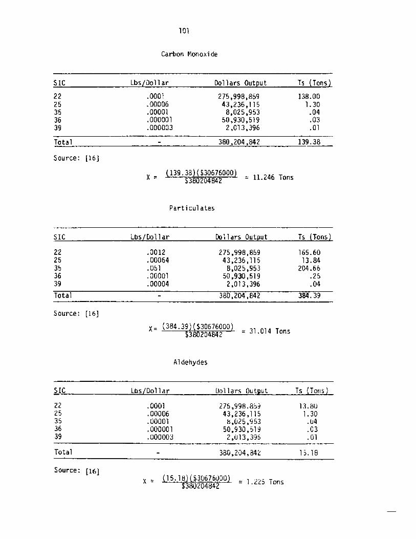
Carbon Monoxi de

S IC Dollars Out ut

. 0001

.00006

.00001

.000001

.000003

139.38Total

X =

Parti cul ates

Do'Ilars Out utSIC

Total 384. 39

X=

Dollars Gut ut

.0001

.00006

.00001

.000001

.000003

Total 15. 18

22

25353639

Source: [16]

2225

353639

Source: [163

2225353639

Source; [16]

Lbs Dollar

Lbs Dollar

. 0012

.00064

.051

.00001

.00004

Ibs Dollar

Aldehydes

275,998,85943,236,115

8,025,95350,930,519

2,013,396

380, 204, 84 2

= 11.246 Tons

275,998,85943,236,115

8,025.95350.930, 519

2,013,396

380,204,842

= 31.014 Tons

275,998.85943,236,115

8,025,95350,930,519

2,013,396

380,204,842

= 1,225 Tons

Ts Tons

138. 00

1. 30.04.03

,01

Ts Tons

165. 60

13. 84

204. 66.25

.04

Ts Tons

13. 80l. 30

.04

.03

.01

1 02

Hydrocarbons

Ts Tons!Lbs/Dollars Dollar OutputSic

15.18Total 380,204,S42

Source: [16]

X = = 1.225 Tons

Solid

Solid waste engineering factors per employee for StC categories

corresponding to the Mississippi Miscellaneous Manufacturing sector were

averaged and multiplied by sector employment. Soli d waste esti mation is

summarized below.

Miscellaneous Mfg. Soli d Haste Factor

Solid Haste Em Year Tons!SIC 1ndus tr

Texti lesFurni ture

Rubber-pl asti cLeatherNone 1 ectri cal mach.Electrical mach.instrumentsMisc. mf .

Tota Avera e sector 1.01

[42]

1090 = Miscellaneous Mfg. employment Appendix A!x 1.01 = Tons/emp/year [42]

1100.9 = Tons/year

2225353639

2225303135363S39

. 0001

. 00006

. 00001

.000001

.OOG003

275,998,85943,236,115

8,025.95350,930,519

013 396

.Zb

.522.6U

.172,601.70

.12

.14

13.801.3

.04

.03

.01

SECTOR 1 8

MATER TRANSPORTATION

Water

The coomercial methodology of Section III-A was used to estimate

Mater Transportation effluent loadings. Maste water flow factors as

shown in Table 2 of Section III-A were not available for the Mater

Transportation sector, necessitating the substitution of average per-

capita water use see Appendix 8, Households!. Waste water flow is given

below.

Waste water flow of 17.5 MGY was applied to net medium eff fluent

concentrations as illustrated in Table 3 of Section III-A to allocate water

effluent tonnages contained in waste water flow. Calculations are sunmarized

Water Transportation Effluents

Waste Water Concentrati on Effluent/ Conversion AnnualEf f I vent MGY MG/I. MGY lbs lbs al Tonna e

303.4782.80

306

15

103

BODChlorineFec. ColiformSus. SolidsNitrogenOil 8 Grease

'I7.5

17.517.517.517.517.5

1167 = Water Transportation employment Appendix A!50 = Gal fons per-capita waste water/day Appendix 6!

58350 = Gallons /day300 = Days/ye a r

17.5 = Million gallons/year MGY!

8.34 2. 190.031

49.000d8.34 2.1908.34 .4388.34 1.095

104

[20]b [23cWeight of 1 gallon water

Air

The South Carolina study aggregated all transpor tation into

one Transport and Storage sector. The non-household methodology of

Section III-B was used in the following computations to allocate total

air emissions to Water Transportation. Total tonnage was found by multi-

plying the adjusted coefficient pounds per dollar! by Mississippi Water

Transportation output.

~0ut ut Percent

Water Transportation $30,635,000Other Transp. 8 Warehousing 36,686,000

4654

Water Transportation Air omissions

Aog. Mi ss.CoefficientAir Pollutant Tonna e

Sources: [l6]

Soli d

The conmercial average per-capita solid waste factor for urban

areas was applied to sector employment to give tonnage of solid waste.

Total pounds were converted to tons as shown below.

Water transportation employment Appendix A!Pounds/day/employee [42]Pounds/dayDays/yearTons/yea r

1167 =x .46 =

~536. 8x 300 =

8885

Ni trogen OxideSulfur Oxide

Carbon MonoxideParti cul atesAldehydesHy droca rbons

. 013

.020

. 019

.003

.004

.00598

. 00920

.00874

.00138

,00184

91.599

140. 921133.874

21.13828. 184

SECTOR 19

OTHER TRANSPORTATION AND WAREHOUSING

Water

The commercial methodology of Section III-A was used to derive

Other Transportation effluent loadings. Average per-capita water use

Appendix 8, Household! was used to estimate waste water flow rate because

engineering factors were not avail able.

Waste water of 10.335 MGY was multiplied by net medium effluent

concentration shown in Table 3 of Section III-A to allocate effluent tonnage.

Calculations are presented below.

Other Transportation Water Effluents

Was te Water Concentration Effluent/ Conversion AnnualEffluent NGY MG L a Ga l lbs b Lbs al c Tonna e

8. 34

3.478Z. 800

8. 348.348.34

30 615

b[20][23]Conversion factor0/ML

Air

The South Carolina study aggregated a'll transportation into Transport

105

BODChl orineFecal Col i formSus. So 1 i ds

NitrogenOil 5 Grease

689x 50

34450

x 300= Ti~lY

10. 33510. 33510.33510.33510.335l0.335

Other Transp. and Whse. employment Appendix A!Gallons per capi ta was te water/day Appendix B!Gal 1 ons/dayDays/yearMillion gal lons/year MGY!

1.293. 018

28.938d1.293

.295

.647

106

and Storage. The non-household methodology of Section I II-8 was used

in the following to allocate total emissions to Other Transportation.

Total tonnage was found by multiplying the adjusted coefficient pounds

per dollar! by sector output Some of the tonnage value may seem too

low, but any transportation carried out in another sector was counted in

the same, Oddly firms invo!+ed with transportation as a busi ness were

included in Other Transportation.

~0ut ut Percent

Water Transportati on $30,635,000Other Transportati on g Warehousing 36,686,GOO

4654

Other Transportation Air Fmissions

Rdj. Hiss.CoefficientAir Pollutant Lbs Dollar Tonna e

Source: [16]

So li d

The average corrmercial per-capita solid waste factor for urban

areas was applied to sector employment to give solid waste tonnage. Total

pounds were converted to tons as shown below.

Other Transportation employment Appendix A!Pounds /day/empl oyee �23Pounds/dayDays/yearTons/year

Nitrogen OxideSul fur Dxi desCarbon Honoxi deParti cuIates

Al dehy desHydrocarbons

.013

. 020

. 019.033.004

689 =x .46 =

~31 6. 9x 300 =

47. 541

. 00702

. 01080

. 01026,00162

.00216

128. 768

198.104188. 199

29.716

39.621

SECTOR 20

COMMUNICATIONS AND PUBLIC UTILITIES

Percent GenerationKi 1owatt Hours

Plant 1Plant 2

6733

I,000,000500,000

Source: Mississippi Power Company

Effluent printouts were available only for plant 1. Plant 2

effluents were estimated by allocating its respective share of total

generation as summarized below.

Communications-Publi c Utilities Effluents

Total

Tonna ePlant 1

Tons aPlant 2

Al 1 oca ti onEffluent

Waste WaterBODChl orineFecal Co 1 i formcSus. SolidsOil and GreaseIron

44.832.019.002

4440.4057.965

.170

.003

33.708.014

.00!

3338.6505.989

. 128

.002

1.331.33

1.33

1.331.331.331.33

Water

The major source of effluent loadings in the Communications and

Publi c Utilities sector is power generating activity, to which there were

two large power generating facilities located in the Mississippi coastal

region. As shown below, plant 1 in 1977 generated 67 percent of electri-

city in the region, receiving about 75 percent of its power from coal.

The other 25 percent was via fuel oil and natural gas. Plant 2 supplied

33 percent of totaI generation using fuel oil exclusively, but has

recently converted to coal.

108

Co er -0006 . 0011.33

' tr3]MGY

The South Carolina study had more sectors in the Coranunications

and Public Utilities category than the corresponding Nissi ssi ppi sector.

However, the only South Carolina sertor with ai r pollution coeffi ci ents

was the Electric Utilities sector which corresponded exactly to the

Mississippi sector. Thus, power generating coefficients were multi p'ii ed

by Mississippi sector output and converted to tons. Technical data

indicated that emi ssions were too low for sulfur oxides and particulates

and revised accordingly [2Sj . Final results are shown below in tons per

year.

Ni trogen Oxi de 9.083Sulfur Oxi des 40000.000Carbon Monoxide 7.445

Particulates 2500.000

Aldehydes 74.450Hydrocarbons 223.349

Sol i d

3002 = Comm. Public Utilities employment Appendix A!x .65 = Pounds/day/employee [42]

1951. 3 = Pounds/dayx 300 = Days/year

=~2 2.695 = Tons/year

The industrial average solid waste factor for urban areas was

used to derive solid waste loadings. The engineering factor was multiplied

by sector output as shown below.

SECTOR 21

EAT[KG AND DRIllKING PLACES

Hater

4706 = Eating Drinking employment Appendix A!x .29 = Fast food proportion [35], [30]

1365 = Fast food employment

761 = Eating Drinking establishments [33].29 = Fast food proportion [35], [30]221 = Fast food establishments540 = Full service establishments

Fast Food Full Service

1365 = Employmentx 133 = Gallons/emp/day [37]

181545 = Gallons/dayx 360 = Days/year

663..>6 = Million gallons/year

540 = Establishments

x 150 = Seats /establishment [36], [30]81000 = Full service seats

x 8 = Gal lonsjseat/day [20]648000 = Gallons jday

x 360 = Days

109= ~233. 80 = Million gallons/year

To estimate waste water flow Eating and Drinking Places were

divided into full service and fast, food categories to utilize available

data sources. Restaurant waste water factors were applied to number of

seats in estimating full service restaurant waste water. Average gallons

per fast food worker was applied to sector employment for fast food waste

flow. Full service and fast food waste water flow were summed to yield

total sector waste water. The procedure is detaHed below, assuming a

360 day year. It i s noted that bars and taverns are frequently licensed

within eating establishments. Mississippi Tax Conmission data suggested

an extremely small percentage of separate drinking places; thus, the

accuracy of the estimation is not impaired [33]-

110

65.356 = MGY Fast food+ 233.280 = NGY Full Service

HlY.I>;E = MGY Eating and Drinking

Total waste water flow of 298.636 MGY was applied to net concen-

tration factors listed in Table 3 Section III-A to allocate effluent

tonnages. The procedure is surrearized below.

Eating and Drinking Places Effluents

Waste Water Concentration E f uent/ Conversion nnuaEffluent MGY NG L a Gal lbs lbs al Tonna e

303.4782.800

8. 348.348.34

306

15

ab [20]

[23]dWeight of 1 gawlon water

¹/NL

Ait

There were no listed air pollution coefficients for Eating and

Drinking places in other studies. Emissions were assumed to be zero.

Sol i d

Solid waste factors for fast food and full service categories

were multiplied by average number of meals and converted to an annual basis.

Sector estimation is suamarized below, assuming a 360 day year.

Full ServiceFast Food

221 = Establishmentsx 692 = Meals/day [33]

152932 = Meals/dayx 360 = Days/year

=~752TW6 = Tons/year

81000x 1.04

842.%ox 2T6iÃFo

36030326.4

*Low side estimate ofrange

BOD

ChlorineFec. Col i formSus. SolidsNitrogenOi! 4 Grease

298.636298.636298,636298.636298.636298.636

37. 359.519

836. 18137.359

7.47218. 680

Seats See waste water!Turnover/seat [3e]Meals/dayPounds/meal [42]Pounds/dayDays/yearTons/year

Fast Food

Full Servi ce

Total Eatin and Drinkin

27527.760 = Tons/year30326.400 = Tons/yearVN~I~5 = Tons/year

SECTOR 22

SERVICE STATIONS

Water

Waste water flow for the Service Station sector was estimated

with the waste water engineering factor of Table 2, Section III-A. The

procedure is given below.

«Pump is defined as underground tankservi cing gasol ine dispensers.

Waste water flow of 102.6 MGY was multiplied by effluent concen-

trations shown in Table 3, Section !II-A to allocate water effluent tonnages.

The procedure is sumnarized below.

Service Station Effluents

Waste Water Concentration E vent/ onversion nnuaE f fluent MGY HG L Gal lbs lbs/ al Tonna e

303. 4782.800

306

15

I 23]Weight of 1 gallon water0/ML

112

285x 3

855x 400

342000x 300

= TK~O0

800 102. 6Chlorine 102.6Fec. Coliform 102.6Sus. Solids 102.6Nitrogen 102.6Oil and Grease 102.6

Service station establishments I 33]Pumps/station [>9j*Total pumpsGallons/pump/day tzo]Gallons/dayDays/yearMi 1 1 i on gall ons/year

8. 34 1 2. 836.179

287.2808. 34 1 2. 8368, 34 2. 5688. 34 6. 418

114

Air

Private household motor vehicle emissions were entered in theService Station sector to minimize distortion of linear assumptionsbetween auto emissions and household income t17]. Input-output metho-dology assumes a proportionate relationship between resource useage anddollar output regardless of output level. However, as household incomeiocreases, automobile travel and, consequently, emissions will increasedisproportionately. Thus, household pollution was charged to ServiceStations because emissions are more linearly related to gasoline salesthan to household income. Household emissions are estimated in Appendix8, Households.

Solid

The average conInercial solid waste factor was used to estimateService Station solid wastes. The procedure is sunInarized below.

1196 = Service Station employment Appendix A!x .46 = Pounds/day/employee [42]

550.16 = Pounds/dayx 300 = Days/year

82.5% = Tons/year

SECTOR 23

WHOLESALE AND RETAIL TRADE

Water

Waste water sewage engineering factors for trade establishments

could not be used because store frontage feet were practically unavailable

for an area as large as the coastal region. Waste water sewage flow was

estimated using average per-capita water use as shown below. Althoughthere are problems with this methodology, no other data were avai lable-

l4178 = Hholesale and Retail employment Appendix A!x 50 = Gallon per-capita water/day Appendix B!

708900 = Gallons/dayx 300 = Days/year~12.6 = Millions gallons/year S1GY!

Waste water flow of 212.67 NGY was applied to net waste water factors

of Table 3, Section tI I-A to allocate effluent tonnages . This procedureis summarized be'tow.

Wholesale-Retail Trade Effluents

aste Water Concentration ff uent Conversion AnnuaEffluent MGY MG L Gal lbs b lbs al Tonna e

30 S.343.4782. 800

306

15

8.34

8.348.34

b[ o]I23]

dConversion factor

BOD 212.67Chlorine 212.67Fec. Coli f. 212.67Sus. Solids 2'I2.67Nitrogen 212.67Oil S Grease 212.67

26.606.370

595'.476d26.606

5.32113.303

Ai r

The South Carolina study did not list air pollution coefficients

for Wholesale and Retail Trade. Unpublished engineering data did allow

an estimation of incinerator particulate for tneHississippi coastal

region totalling 20 tons �5j,

Soli d

Solid wastes were estimated using engineering factors based upon

units of 1000 square feet of interior store space. Total square footage

was estimated by dividing gross sales including cost of goods sold! by

average retail/wholesale sales per square foot for typical types of

stores. Calculations are sumnarized below.

Gros s 5 a'I es

$203,965,000 Wholesale/retail sales adjusted for costo f goods sol d, Appendi x A!

x 4.2553 Cost of goods sold multiple [38]

�.2553 = 1/.235, where.235 equals margin!

$79 Sales per square foot, average of stores under $1 mi'Ilionand over $1 million [43]

= 10,986,484 square feet

2= 10986. 5 �000 f t !

Waste Factor

10,986.5 = 1000 ftx 1.2 = Pounds/1000 ft /day [4z]TTTFFY = Pounds/dayX 300 = Days/year

= ~Pi~iT = Tons/year

SECTOR 24

FINANCE, INSURANCE, AND REAL ESTATE

Water

Waste water sewage f]ow for the Finance, Insurance, and Real Estate

sector is based upon the numoer of offices as shown in Table 2, Section

III-A. For purposes of estimation it was assumed that on the average

there were two employees per office unit.

3789

21837

x 10T8895

x 300= 5.565'

Waste ~ater sewage flow of 5.685 MGY was multiplied by net concen-

trations per effluent to estimate tonnages of water effluents. Estimations

are sunmarized below.

Fl RE E f f 1 uents

Waste Water Concentration Ef fl uent/ Convers i on AnnualEffluent MGY MG L a Ga I 1 bs lbs al Tonna e

8. 343.4782. 800

306

15

8. 34

8.348.34

116

8OD 5.685Chlorine 5.685Fec. Colif. 5.685Sus. Soli ds 5.685Ni trogen 5. 685Oil l! Grease5. 685

bt:ZOJ[23jConversion factor0/ML

FIRE employment Appendix A!Employees/officeOfficesAverage was te water/day/o f f i ce [20]Was te wa ter/dayDay/yearMi1 lion gall ons/year MGY!

.711

.01015.918

.711

.142

.356

117

Solid

Solid waste consisted mainly of paper waste and was estimated

using the average comnercial solid waste factor. The procedure is given

below.

3789 = FIRE employment Appendix Ajx .46 = Pounds/day/employee �2]

1742.94 = Pounds/dayx 300 = Days/year= 2261. T = yooa/year

SECTOR 25

HOTELS, MOTELS, AND LODGING

Water

Waste water flow for Hotels, Motels, and Lodging was estimated

using the waste water factor of Table 2, Section III-A. The procedure

is given below.

Waste flow of 61.628 MGY was multiplied by effluent concentrations

shown in Table 3 of Section III-A to allocate effluent tonnage.

Hotels. Motels, and Lodging Effluents

Waste Water Concentration Eff]uent/ Conversi on AnnuaEf fluent MGY NG L Gal Ibs 1bs al Tonna e

30 8. 343.4782.800

306

15

8.348.34b. 34

b[20][23jConversion factor

118

4600 =x .59 =

739 =

x 75=

x 300 =

61.628-

BOD 61.628Chl orine 61. 628Fec. Col i f orm 61. 628Sus. Solids 61.628Ni trogen 61.628Oil 5 Grease 61.628

Total rooms. Miss. gulf coast [s]Average yearly occup ancy [28]Rooms occupiedGallons/day/room [zojGallons/dayDays/yearMillion gallons/year MGY!

7.710.107

172 559d7.7101.5423.855

119

Soli d

Solid wastes were derived using the appropriate engineering factorfor hotels and motels as shown in Table 4, Section Ill-C. All classes oflodging places including the medium class were averaged to give 2.2 poundsper room daily� .

2739 = Rooms [Sj, [28]x 2.2 = Pounds/day/room [42j

703. = Tons/year

SECTOR 26

MEDICAL SERVICES

Water

Waste water flow for Medical Services was estimated using the

average waste water factor of Table 2, Section III-A. The number of beds

was based upon a telephone survey of 9 major medical facilities. Using a

reported annual occupancy rate of 92 percent, there were approximately

2,062 beds in use on an annual basis. R 365 day year was assumed in the

calculations below.

Waste water flow of 120.421 MGY was applied to appropriate effluent

concentrati on factors to allocate effluent tonnages, as shown below.

Medical Services Effluents

Waste Water Concentration Effluent/ Conversion AnnualEffluent MGY MG L Gal lbs los al Tonna e

8. 343.4782. 800

306

l5

8.348. 348. 34

b {20]Conversion f'actor0/ML

12n

BODChl orineFec. Coli form

Sus. SolidsNitrogenOil 8 Grease

2062 = Hospital beds telephone survey!x 160 = Average gallons/bed/day {20]~~92' G = Gallons/dayx 365 = Days/year

120.421 = Million gallons/year MGY!

120 42112U.421120.421120.421120.421120.421

15.065.210

337.179d15.065

3.0137.533

121

Sol id

Solid wastes were estimated using the per-bed engineering factor

of Table 4, Section III-C, as shown below,

2062 = Beds telephone survey!x 8 = Pounds/bed/day t42]

16496 = Pounds/dayx 365 = Day/year

= 330 ~.35 0 = Tons/year

SECTOR 27

EDUCATIONAL SERV! CES

Water

Waste water flow was estimated with a per-pupil factor as shown

in Table 2 of Section I I I-A. Estimated number of students in the coastal

region based upon average dai ly attendance is given in the table below.

Number of Students

School or District Avera e Dail Attendance

Source: [45]

Average daily attendance of 56,287 was multi plied by the average

engineering factor, assuming a 220 day year. That is, the academic year

was assumed to be a nine month sessi on plus two months of sueoer school

ZO days per month!. The inclusion of all students in the sumner term

helped to account for some college and junior college attendance not

covered in the table.

122

HancockBay St. LouisHarrison Co.BiloxiGulfportLong BeachPass Christi anJackson Co.Mass Point

Ocean SpringsPascagoula

County Total

17511811

923069816774330713756276648240098291

56287

123

Waste water flow of 173. 364 MGY was then applied to the effluent

concentration listed in Table 3, Section III-A.

Educational Services Effluents

Waste Water Concentration Effluent/ Conversion AnnualEffluent MGY MG L Gal lbs lbs al Tonna e

173.364

173.364173.364173.364I73.364173.364

8.34303.4782.800

8. 348.348.34

306

15

'Izo][23]

cdConversion factor0/ML

Soli d

The per-pupil solid waste factor of Table 4, Section III-C was

applied to number of students to estimate solid waste tonnage.

56287 = Average dai ly attendance I45]x 2. 1 = Pounds/pupil/day f42!

170202.7 = Pounds/dayx 220 = Days/year

= 13002.297 = Tons/year

BODChl ori neFec. Coliform

Sus. Soli ds

NitrogenQil 8 Grease

56287 = Average daily attendance [4S ]14 = Gallons/pupil/day [zo]

788018 = Gallons/day220 = Days/year

173.364 = Million gallons/year MGY]

21 . o49

, 302485. 419d

21.o894. 317

10. 844

SECTOR 28

OTHER SERVICES

Water

Waste water flow for Other Services required residual allocation

because the heterogeneity of services and the data required thereof caused

the use of waste water engineering factors to be impractical. The approach

taken was to subtract water flows of all other corrlnercial sectors from the

total corrmrercial water magnitude discussed in Section III-A. This procedure

is given below.

Corrmercial Sector Waste Water Except Other Services

Number Sector Waste Water MGY

Total Water Flow 1032.760

Source: [203, [2>!

44l 7.895 Corrmercial flow, sectors 18-19. 20-29 Section III-A}

- 1032.760 Non-Other Svc. flow, sectors 18-19. 20-Z7,Z9= 33385. 35 Other Services flow, sector 28 MGY!

Waste water flow of 3385.135 MGY was multiplied by appropriate

concentration factors to allocate effluent tonnages as shown in the

I24

18

192122232425262729

Water transportationOther transportationEating-drinkingSer vice stationWholesale-reta i 1FIREWote1 s-motel sNedi ca 1 servi cesE ducat i on a 1 se rvi cesState-local gov't

17.50010.335

298.636102.600212.670

5.68561.628

120.421173.364

29.910

125

following. Although total waste water loadings by the Other Services

sector may appear high, this sector includes many di verse, water-consuming

businesses such as laundromats and swiping pools.

Other Services Effluents

Haste Hater'MGYEffluent

3385.1353385.135

3385. 1353385. 1353385.1353385.135

303.4782.800

306

15

b [20][231

cd Conversion factorP/ML

Solid

The cotImercial average solid waste engineering factor for urban

areas shown in Table 5 of Section III-C was used to estimate sectoral solid

waste tonnage, as shown below.

13156 = Other Services employment Appendix A!x .46 = Pounds/emp/day [42]

6051.76 = Pounds/dayx 300 = Days/year= 907.764 = Tons/year

BODChl ori neFec. ColiformSus. Solids

NitrogenOil and Grease

Concentration Effluent/ Conversion AnnuaMG L a Gal lbs lbs

8.34 423.4805.887

947d.3788.34 423.48O8.34 84.696

8.34 211. 740

Water

Waste water flow was estimated using the average office factor

shown in Table 2 of Section III-A. For government, one person per office

was assumed.

9970 = Sta te- Loca 1 Gov ' t emp 1 oyment Appendi x A!x 10 = Average gal lons/emp/day [2o]

99&0 = Gallons/dayx 300 = Days/year

29.91 = Million gallons/year MGY!

Waste water flow of 29.91 MGY was multiplied by the appropriate

effluent concentration factors shown i n Table 3 of Section I II-A to allocate

effluent tonnages.

State-Local Government Effluents

Waste Water Concentration Effluent/ Conversion AnnuaMGY Gal lbs lbs al Tonna eEffluent

303. 478

2. 80030

6

15

[20][23]Conversion factor

aP/ML

126

BODChl ori neFec. ColiformSus. Sol i ds

NitrogenOil and Grease

SECTOR 29

STATE AND LOCAL GOVERNMENT

29.9129. 9129.9129.9129.9129.91

8.34 3.742.053

83.748d8.34 3.742

8.34 .7498.34 1.841

127

Sol i d

The commercial average solid waste factor for urban areas was applied

to sector employment to yield total solid waste, as shown below.

9970 = State- Local Gov't employment Appendix A!x .46 = Pounds/emp/day [42]

4586.2 = Pounds/dayx 300 = Days/year

66863 = Tons/year

SECTOR 30

HOUSEHOLDS

Water

Mi s s i ss i ppi Coas ta 1 Reg i on Popul at i on

1980 Po ulationb1975 Po ulationaCount

21, 442148,247137,376307,065

HancockHarr ison

JacksonTota 1

18,100146,8001G5,800270,700

[49][ze]

Estimated 1977 Po ulation

Population change, 1975-1980Years

Ch an ge/yea rYears

Change, 2 yearsPopulation, 1975Estimated population, 1977

36365

7273X 2

14546+ 270700

85246

128

Household waste water flow of 5205.740 MGY was estimated by applying

1977 population to average per-capita waste water loadings. The following

procedure gives an approximation of average residential waste water, assuming

that 20 percent of total uSe iS COnSumed Or recycled [ZS] Per-capita waSte

water use is based upon the average of these separate studies.

129

Avera e Per-Ca ita Waste Water UseTotal Use

~Stud255246260

Bailey Study, [1]Reid Study, I40]

Average family 4 per familyAverage per-capi ta

25464

Gallons/person/day I I], I11], [4o]Waste water proportionGallons/person /day/waste waterPopulation Mississippi coastal region ~49] ~z6]Gal 1 ons/day/was te waterDays/yearMi llion gallons/year MGY!

64 =x .8=

50 =

x 285246 =14262300 =

x 365 ==55~~5, 5I

As discussed in Section III-A, we now have waste water flow forhouseholds and need to estimate effluent tonnages. The sum of conIiiercialeffluent allocations was subtracted from its combined conmiercial and house-hold loadings. Total commercial and household effluent tonsages were foundby adding printout and non-printout treatment faci lity effluent loadings.This procedure is suranarized below.

Household Effluent TonnagesHousehold

Effluent Tons/ rMAWPCC Faci 1 i tyTotal Tons ear

AllocatedComme rci al Tons r

Effluent

1226. 83916.755

26787.0845929.190

248.748601.958

b I 231 ~ [20]4/ML

Air

Using the methodology of Section II I-B the correction factors forair emissions in Equation 2 were derived to regionalize the mean emissionfactor's in order to estimate private vehicle pollution in tons. The

BOOChlorineFec. ColiformSus. SolidsNitrogenOil and Grease

561. 9197. 812

12370. 076561. 91911~.365280.997

664.9208.943

14417 008b5367. 27 1

136. 383320. 961

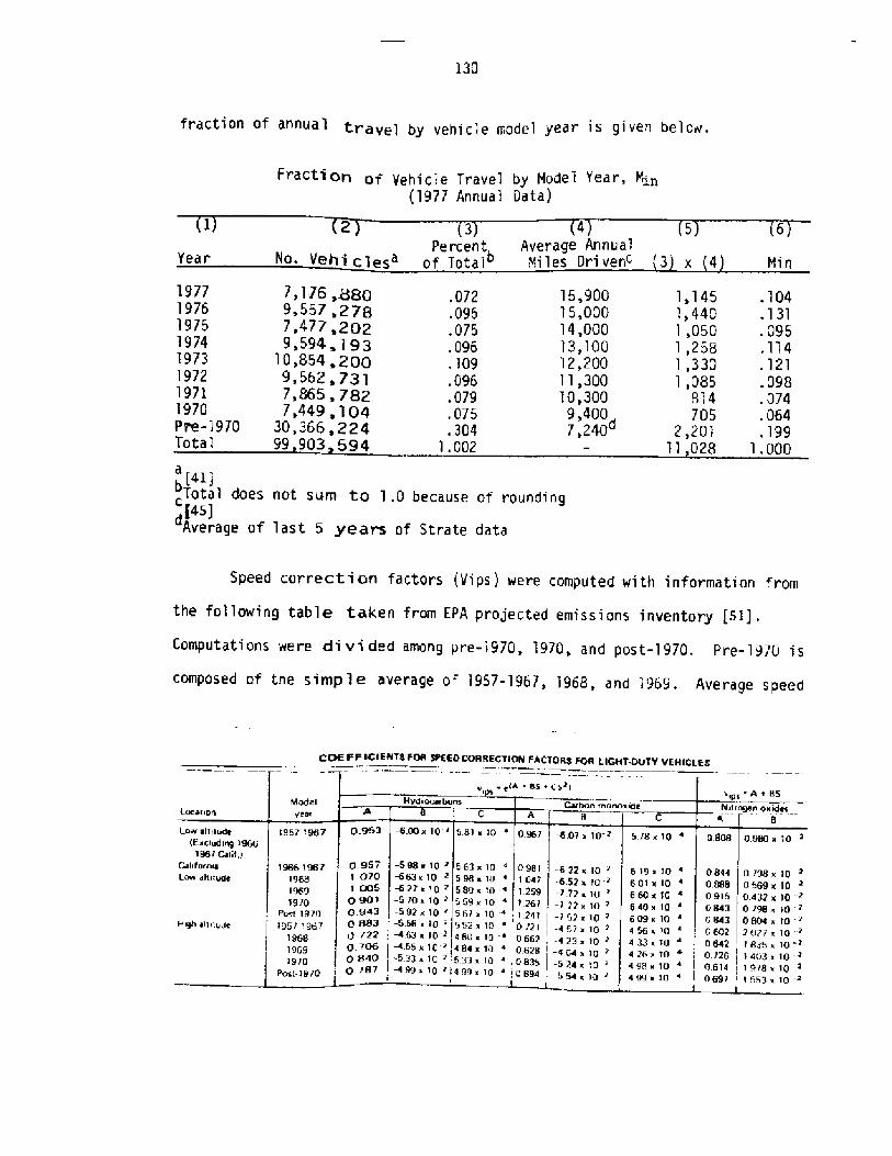
131

S! is assumed to approximate the national average of 45 miles per hour and

includes both highway and city travel. The Nississie ssissippi coastal region falls irit~

the category of low altitude, non-California.

ydrpcarbons . y e A + BS + CS !ips

where:

5 = average speedA, 8, and C from table

P re-1970

[i PPg + - . 063!�5! + . 000586�5!' Jips

yi , = .53

1970

y[9Q1+ �.0o7!�5!+.000559�5!'!lps

V., = .59

[ 943 + p592! �5! + .000567�5! ]i ps

y,- = .56

�! Carbon Monoxide: y ipswhere:

5 = Average speedA,B, and C from table

Pre-19705.87 x 10 "

C = 6.01 x 10 "6.60 x 10 "6,13 x 0

-6.07 x 10-~8=-652x102

.953

A = 1.0701.005TlR5

. 967A = 1.047

l. 259~1. 09

-6.00 x 10 'B = -6.63 x 10 i

-6.77 x 10 '-6.3 x 10

5.R1 x 10 "C = 5.g8 x 10 "

6,80 x10"

132

y {1 ~ 091 + ~ 0677! �5! + 00061 3�5! ]1PS

V1 S = .49

y � {1.267 + �. 0772! �5! .000040�5! ]lps

V, ~ .401PS

Post-1970

e {1 ~ 24'1 + , 0752! �5! +, 000609�5! ' ]1PS

401ps

�! Hi trogen Oxides: V. = A + BS1PS

where:

S = Average speedA and B fr om table

Pre-1970

V. = .87 + .0066!�5!

"1ps = 'l.167

1970

V. = .843 + .00798!�5!

V1ps = i.202

Post-!970

V. = . 843 + . 00804!�5!iPS

V; = i.205

. 808A = .888

.915~80

.980 x 10 ~B =,569 x 10 '

.432 x l0 '

.660 x 10

133

Temperature correction factors l;pt! are presented in tne

following table where t equals ambient coastal temperature. The finalcolumns will be used later to determine the hot/cold operation factor

Ri ptw ! The ave rage ambi ent tempera ture for the Ki s s i ss i pp i coas ta1region for 1977 was 67' Farenheit [34]. This temperature falls withinthe EPA temperature band �0'-80'! governing the temperature correction

factors listed in the table. Computations were based upon two basic

engine types: catalytic and non-catalytic. For purposes of estimationit was assumed that catalytic convertors were common to vehicles only

after 1975 [50]. Non-catalyst factors were applied to pre-1975 model

years. Light-Duty Vehicle Temperature Correction FactorsAnd Hot/Cold Vehicle Operation Correction Factors

For FTP Emi ssion Factors

Source: [51]

�! Carbon Monoxide:

Zi pt 0743�7 ! + 6 58

Zipt = 1.689

Zi t = 1.099

l34

� ! Hydro ca rbons;

Z t = -.0304�7! + 3.25ipt

Zipt 1'2132

~Cata! st

» W! 'ipt

t = 1.0529

�! Nitrogen Oxides:

~Cata1 st 2;>t = � .0060�7! + 1.62

Zipt 1 118

1pt

Zi, = 1.O51S

Ri ptw

where:

w = Percentage of cold operationf t! = Computed from previous table

The hot/cold vehicle operation correction factor Ri t�! adjusts

vehicle emissions during three phases of typical engine use: �! a cold

transient phase start-up after long engine-off period!, �! a hot transient

phase start-up after short engine-off period!, and �! a stabilized phase

warmed-up operation! [50]. The following two formulas specify en!ission

corrections based upon the assumption of national averages that 20, 27, and

53 percent of all vehicles operate in cold, hot transient, and stabilized

phases, respectively, for automobiles with catalytic converters after 1975.

For non-catalytic pre-1975 vehicles the hot-transient phase is combined

with stabilized phase to yield 20 percent cold operation and 80 percent

hot operation The formulas for both categories are given below. The

terms f t! and g t! were derived from Columns i! and �! of the previous

taole of temperature correction factors.

Pre-1975 Non-Catal st Vehicles

I35

Post-1975 Catal tic Vehicles

iptw

where:

x = Percentage of hot start-up

g t! = Computed from previous table

The above functions are based upon national average conditions as

specified earlier. If the study area is exactly the same, the correction

factor reduces to one and has no effect upon ai r emissions. This, of

course, would be a naive assumption. An EPA s tudy shows that the higher

the proportion of urban population, the more likely are vehicles to i ncrease

cold operation during afternoon rush when work-to-home tri ps are at a peak

and vehicles have been standing idle for 8 hours 0], Using this principle,

cold operation for the Mississippi coastal region was adjusted by multiplying

the national average cold operation factor times the ratio of regional to

national urban population proportion, as shown below.

Re ional Urban Pro ortionNational Urban Proportion x National Cold OPeration

.77735 x 47 = 49

where: .47 = .27 + .20

Source: [47]

1.048 x .20 = .21

The adjusted hot/cold proportions for catalytic and non-catalytic

vehicles are given below.

136

Cold w!Hot Start-up x!

Hot Stabilizea

21%28%51K

A~dusted

Cold w!Hot

21%

79%

Using the adjusted hot/cold proportions in the correction factor

formuIas Rip«!, the hot/cold temperature correction factors for airemissions were computed as shown be1ow.

�! Carbon Nonoxi de:

Pre-1975

i ptw

Post-1975

Riptw =

"iptw =

�! Hydrocarbons:

Pre-1975

i ptw .99

Post-1975

iptw

Riptw = ' G3

�! Ni trogen Gxi des:

Pre-1975

Riptw =

137

Post-1975

R.i ptw

Riptw = 1 01

At this point we have derived the following correction factors ofEquation 5, Section III-B: M, V, Z, and R. The uncorrected mean emissionsfactor in grams per mile Cipn! for each pollutant is given in the tablebe 1 ow.

Carbon Monoxide, Hydrocarbon, and Nitrogen OxidesExhaust Emission Factors For Light-Duty, Gasoline-Powered VehiclesExcluding California-For Calendar Year 1977

Based on 1975 Federal Test Procedure!Nitrogen

oxidesCarbonMonoxide H drocarbons

Location andmodel ear

mi

Source: [51!

The mean emissions factors C! were multiplied by appropriatecorrection factors thus derived in order to regionalize the estimation ofair emissions tonnages. The sum of the composite emissions factors Enstw x!!in coastal regions for all pears yields total emissions in grams permile. The procedure is applied to carbon monoxide, hydrocarbons, and nitro-gen oxides in the next three tables. Emissions of particulates and sulfuroxides do not require correcti on and are computed in the final table.

Low AltitudePre-1968

1968196919701971197219731974197519761977

98.079.677.466.063.547.045.043.010. 8

9.99.0

60.949.448.141.039.429.227.926.7

6.76.15.6

9.29.27.37.35.94.7

4.44.11.4

1.Z1.0

5.75.74.54.53.7

2.92.7Z.50.90.7

0.6

3. 34 Z. 074. 32 Z.t85. 08 3.154. 35 Z. 704. 30 2.674,55 2.833.9 2.43.7 2.33.3 2.03.2 2.02.0 'I. 2

l38

Carbon Monoxide

Model Year

21.60Com osite Emissions: Grams Per Mile

source: [5l]

Hydrocarbons

Model Year

Gr ms er Mile 2 6~Source: [51]

Nitrogen Oxides

11itw x EnstwModel Year Cin

Com osite Emissions: Grams Per Mile

Source: [51]

19771976197519741973197219711970Pre-1970

19771976197519741973197219711970Pre-'1970

1977197619751974197319721971

1970Pre-1970

9.0

9.910. 843.045. 047.063.566.0

85.0

1.01.21.44.14.44.75.97.38.6

2.03.23.3

3.73.94.55

4.3

4.354.25

. 104

.131

. 095. 114

. I 21

. 098

.074

.064

.199

.104

.'131

. 095

.114

. 121

.098

.074

.064.199

.104

. 131

.095

.114

.121

.098

.074

.064

.199

.4

.4

.4

.4

.4

.4

.4,4.4

.56

.56

.56

.56

.56

.56

.56

.59

.53

l.2051.2051.2051.2051.2051.2051.2G51.2021.167

1.691.691.691.101.101.10].10

1. 10

1.10

1. 211. 211.211.05

1.G51.051.0>1.051.05

1.121.121.1'

1.051.051.051.051.051.05

.94

.94

.995

.995

.995

.995

.995

.995

1.031.031.03

.99

.99

,99.99.79.99

1. Ol1.011.01

9999

.9999

.99

.99

.eo

.v2

.652.15

2.382.022.061.85

9.07

.07

.11

.09

.27

.31

.27,25.29.94

.28

.57

.43

.53

.59

.56,40.35

1,03

139

Total Mi les Traveled Regi stered Pri vate Vehi clesMississippi Coastal Region 1977

Mi lesTraveled

l977

Proportion of Total Passenger Avg. AnnualModel Total Vehicles, MS mi. Traveled/Year Annual Travel Coastal Re ion 1977 veh model r

236,258,100280, 725,000l 90,022,000213,372,800207,456,000158,2r 2,ouO106,901,90085,953,600

205,847,680

197719761975197419731972197'I

1970Pre-1970

.104

.131

.095

.114

.121

. 098

.074

.064

. 199

15,90015,00014,00013,10012,00011,30010,3009,4007,240

14. 85918,715l3,57316,28817,28814,00210,5739,144

28,43Z

1,686, 759, o60142,8741.000Total

[45][32], [Sl.][46], [51]

kousehol d Secto r Ai r Po1 1 uti on

Mississippi Coastal Region, 1977

Compos i te F.mi s s i onsa

AirPo 1 1 utan t

Carbon Monoxide

HydrocarbonsNi trogen Oxi desParticulatesSulfur Oxides

21.602.60

4,74.60.23

36, 4 34, 009, 0884, 385, 575,1687,995,2a0,8831,012,055,808

387,954,726

1, 686, 759, 680 40,160.9454,834.1888,813.0961,115.582

427.640

f[51], See previous discussion1 Ton = 907,200 gramsNo regional correction required

Total miles traveled in 1977 by privately-owned passenger vehicles

are given below. Total miles traveled were then multiplied by composite

emissions factors E! in grams per mile to yie'Id total grams of air emissions.

This procedure is summarized in the final table. Total grams were converted

to tons to complete the estimation of household air emissions. Particulates

and sulfur oxides did not require regional correction and were estimated

directly from their composite emission factors. As explained earlier,

household air pollution was entered in the Service Station sector because

of the more linear relationship between gasoline sales and automobile

us age.

140

Sol i d

The solid waste factor for urban areas with a population density

of 10-200 persons per square mile was applied to estimated 1977 Mississippi

coastal population to give solid waste tonnage. The upper limit of the

range for the waste factor was used since population density approached

200 per square mile [34j. A 365 day year is assumed.

285246 = Population See Households, Water!x 3.1 = Pounds/day/person [42]= 884262.6 = Pounds/dayx 365 = Oays/year

= 161377.920 = Tons/year

BIBLIOGRAPHY

141

B IBL! OGRAPHY

Ba i 1 ey, R., Benoit, R. J., Dodson, J. L., Robb, J. M. andWallman, H. A Stud of Flow Reduction and Treatment of WasteWater from Househol ds. Water Pollution Control Resear ch Series,

05 FKE, Advanced Waste Treatment Research Laboratory, Cincin-nati, Ohio, December 1969.

Benarde, Melvin A. Our Precarious Habitat. New York: W. W. Norton andCompany, 1970.

4. Blay lock, James E. and Jones, Lonnie L. An Analysis of Economic-Envi ronmental Interrelations on t e Lower Rio Grande Re ion ofexas. exas grs cu tura xper>ment Stat>on. exas

University. July, 1973.

5. Cartee, Charles P., Wi lliams, D. C., and Murray, Nell 0. A Histori aland Pro 'ected Anal sis of Travel and Tourism in the Mississi i

u f P annwfn Re ~ on.

6. Carter, A. P. and Brody, A., eds. A li cati ons of In ut-Out ut Anal sis.Amsterdam, Holland: North-Ho an Pu is >ng Co.,

7- Carter, Clare E,, Fink, Linda L., Teaf, Christopher M., and Herndon,Roy C. Hazardous Waste Surve for the State of Florida. FloridaResources and nvlronmenta na ysls Center. or> da State Uni ver-sity. October, 1977.

Consulting Engineers. Pascagoula, MS' 1977.8. Compton

9. Department of Ecology. A Re ort on Industrial and Hazardous Wastes,State of Washington, 1974.

10. Dolan, Edwin G.Crisis.

11. Dorfer, C. N. and Becker, E. Public Water Su lies at the 100 Lar estCities in the United States, S. Geo oglca Survey, WaterSupply Paper 18 2, U.S. Government Printing Office, Washington,D. C., 1964.

2. Bell, Frederick H. Benefits From Water Pollution Abatement Coastal Waters.Report No. NCWQ 75/88-Vols. 1-2. Florida State University.Department of Economics. April, 1976,

143

12. Feld, Sidney, and Renholm, Niels. Economic Growth and Generat'io'n ofWaterborne Wastes. University of R ode Island. Marine Tech-

13. Hamilton Standard Division of United Aircraft Corp. Develo mentDocument for Effluent Limitations Guidelines an Standardsof Performance: Fee ot In ustr . Draft prepare or nvi ron-menta Protection Agency . June, 1973.

14. Issard, Walter. Ecolo ic-Economic Anal sis for Re i onal Develo ment-New York: The Free Press, 972.

15. Issard, Walter and Langford, Thomas W. Re ional In ut-Out ut StudCambridge, Mass.: The MIT Press, 1960.

16. Johnson, Manuel H., Jr. An Assessment of the Im act of Nuclear-Power Plant Construction and 0 eration on Smal Re ions.Unpub is ed Doctora Dissertation. Tallahassee, F orida .F 1 o r i da S ta te University, 1977.

17. Laurent, Eugene A.,and Hite, James C. Economic-Ecolo ic Anal sisin the Charleston Metro olitan Re ion: n In ut-Out ut tudReport No., Water Resources Researc Institute, emsonUni versi ty, 1971.

18. Leontief, Wassi ly. In ut-Out ut Economics. New York: Oxford UniversityPress, 1966.

19. Lundberg Survey, Inc. Petroleum Marketing Statistical Service. NorthHollywood, California, 1977.

20. Metcalf and Eddy, Inc. Wastewater En ineerin . New York: McGraw-Hill,Inc., 1972.

21. Micro-Methods Analytical and Engineering Service Co. Pascagoula,Mississippi, 1978.

ZZ . Mills, Edwin S . The Economics of Environmental uali t . New York:W. W. Norton and Co., 1978.

23. Mississippi Air and Water Pollution Control Commission. NPDES SelfMoni torin S stem Data Su<engr Re ort. Unpublished ComputerPrintout. Jac son, ississippi: arch, 1978.

24. Mississippi Air and Water Pollution Control Commission. "Statistics:Functional Operation and Maintenance Status for ExistingWastewater Facilities for the Mississippi Gulf Coast Area."Jackson, Mississippi, 1977.

25. Mississippi Air and Water Pollution Control Commission. UnpublishedEngineering Factors and Data for the Mississippi Coastal Zone.Jackson, Mississippi, 1977.

Po ulation b Count , A e, Sex, and Color: 1960, 1970 and Pro-'ections to . Bu etin . ississippi State University.

l44

21. Mississippi Employment Security Con+i ssion. Research and StatisticsDepartment. Benchmarks: 1970-1977. Jackson, Mi ss i ssippi. Apri 1 .1978.

28. Mississippi Gul f Coast Innkeepers Association. Biloxi, MS, 1977.

29. Mississippi Research and Development Center. Mississi i ManufacturersDire tor 1978. Jackson, Mississippi, 1977.

30. Mississippi Restaurant Association. Statistical Division, Jackson,Mississippi, 1979.

32. Mississippi State Motor Vehic]e Comptroller's Office. "County PostingSheet. " Jackson, Mississippi, 1977.

omputer Printout. ac son, ississippi. anuary

Division of Research, College ofsippi State University, 1977.

34.

35. National Restaurant Association. "RAB Instant Background; Drive-In andFast Food." Profi'les of Leading Categories of Business. Chicago,Illinois, 1976.

36. National Restaurant Association. Tableservice Restaurant 0 erationsRe ort '77. Second Annual Repor or t e nate tates. icagq,

1 n015, 1977.

37. Nation's Restaurant News. "Water Weapon in Fast Food Zoning Fight."May,, p. 14.

38. Nissan, Edward, Daniel, Donnie L., Williams, D. C., and Green, TrellisG. Linka es Between the Econom and the Environment of theCoastal Zone of Mississi i Part 1: In ut-Out ut Mode . Bureauof Business Research. University of Southern Mississippi.March, 1978.

39. Office of the Director. Mississippi Research and Development Center.Regional Office. Gulfport, Mississippi, 197B.

40. Reid, G. A. "Protection of Future Municipal Water Requirements."Southwest Water Works, S. 46:lB, 1966.

41. R. L. Polk and Co. Motor Statistical Division. Detroit, Michigan+ 1977.42. Salvato, Jr., Joseph R. Envi ronmenta'l En ineerin and Sanitation.

2nd. Edition. New Yor ; o n i ey Sons, Inc-,

31. Mississippi State Ki ghway Department. Mi ssi ssi i Count Traffic Ma s,1976 ADT. Transportation Planning Division. Jackson, Mississippi.NNove~ Ner, 1976.

145

43- Scher, Jay, Ed. De artment of S ecialt Store Merchandizin and0 eratin R lt f 19 . ew Yor : Nationa Retai Mer-

iation Financial Executives Division, 1 976.

45. State Super i ntendent of Public Education, Mississippi Department ofEducation. Annual Re ort and Reconmlendations of the StateSu eri ntendent of Public Education . Jackson, Mississippi,1

46. Strate, H. E. Nationwide Personal Trans ortation Stud -Annual Milesof' Automobile Travel. Report Number 2, U.S. Depar tment ofTransportation. Federal Highway Admini strati on. Washington,D. C. April, 1972,

47. U. S. Bureau of' the Census, Department of Commerce. StatisticalAbstract of the United States: 1977. 98th Edition� . Washington,D. C.; Government Printing Office, 1977,

48. U. S. , 1914. Vol . I,C Government

Department of Agriculture� .Part 24. State and CountyPrinting Office, 1974.

Department of Consnerce. Bureau of the Census. ~Po ulationEstimates. Estimates of the Po ulation of Mississi i Countiesan Metro o itan regs: Ju , an . eriesNo. -2 . as inton, : Government Printing Office.October, 1976.

49. U. S.

Environmental Protection Agency, Office of Air and WasteManagement, Office of Air guality Planning and Standards.Com ilation of Air Pollutant Emission Factors. PublicationAP- 2, Part A. Second Edition. Research riangle Park, NorthCarolina, 1976.

50. U. S

Environmental Protection Agency, Office of Air and WasteManagement, Office of Air equality Planning and Standards.Com ilation of Air Pollutant Emission Factors. PublicationAP-42, Part B. Third Edition. Research Triangle Park, NorthCarolina, 1976.

51. U. S.

52. Victor, Peter. Pol lution: Econo and Environment. London: GeorgeAllen and Unwin, Ltdn n 972.

David, and Benstock, Marcy . Water Wasteland. New York: BantamBooks, 1912.

53. Zwick,

44. Soil Conservation Society of America. "A Primer on AgriculturalPollution." Journal of Soil and Water Conservation. Vol. 26,No. 2 March-Apri , , pp.