Linear-time Encodable/Decodable Error-

Correcting Codes

Some results from two papers of M. Sipser and D. Spielman1

1Much of the technical wording within is either taken verbatim or paraphrased from [SS96; S96]; see references.

Coding for Low-Power Communication Across Noisy

Channels

• Static on the line / Game of “Operator” (Spielman’s lecture).

• A coding solution: “A” as in “Apple”, “B” as in “Baseball”, …”Z” as in Zebra.

(Encode)

Messages (live in low-d space)

Codewords (live in high-d space) =

Message Bits + Check Bits + (Decode)

Diagram for codeword space inspired by digital signature lecture at MIT earlier this year

minimum distance bound

Motivation

• Recall one question answered in professor Spielman’s lecture:

• Q1: Do there exist families of codes which as block length grows realize: – constant information rate / – bounded relative minimum distance

• A: Yes! (e.g. Justesen’s explicit construction)

• Q2: Can we construct such a family of codes with linear time algorithms for encoding AND decoding a constant fraction of error?

• A: Yes again!

)( n

r n

Goals

1. Describe randomized and explicit constructions of families of asymptotically good error-correcting codes

2. Describe linear-time encoding and decoding algorithms for these codes– Sketch proofs of correctness for the decoding

algorithms– Motivate why these algorithms are in fact

linear-time

Sights and sounds along the way…1. Linear-time decodable error-correcting

codes (built from expander graphs and existing code)

• Randomized construction• Explicit construction

2. Linear-time encodable/error-reducible Error-reduction codes (also from expander graphs and existing code)

• Explicit construction

3. Linear-time encodable/decodable error-correcting codes (from error-reduction codes)

…and mathematical flavors

• Graph theory– Clever correspondences between graphs and codes, graphs

and graphs. – Expander and regularity properties of underlying graphs

used to establish • minimum distance bounds • correctness of decoding algorithms

– Regularity also used to show rate, linear-time

• Probability– The “probabilistic method,” or, a way to prove existence

theorems non-constructively– How to identify properties of randomly constructed objects

Models of Computation for Linear-Time1

• Cost of Memory access / Bit-wise operations (as a function of argument size n):

– Uniform cost model => 1 time unit– Logarithmic cost model => log n time units

• Machines for sequential decoding algorithms– Graph inputted as a set of pointers; each vertex indexes a list

of pointers to its neighbors2

• Pointer Machine (constant degree directed graph)• RAM

• Boolean circuits for parallel decoding algorithms– Size (= # wires)– Depth (= longest path length in circuit digraph)

2 [SS96, p1713]1 [SS96, p1710-11]

Important things to recall• Linear Codes: codewords form a vector space• Gilbert-Varshamov bound: “Good” linear codes exist for sufficiently long

block lengths • Graphs G = (V, E)• Expander graphs (Mohamed’s lecture)

– All minority subsets of vertices have many (external) neighbors (large “boundary”):

Expansion factor =

• Polynomial-time constructible infinite families of k-regular Ramanujan graphs (Mohamed’s lecture)1

– Realize maximum possible “spectral gap” (~expansion)– Explicit construction of Lubotsky-Philips-Sarnak/Margulis using Cayley graphs2

|||)(| UcU c

1 [LL00 p1]

• “Unbalanced”, (c,d)-regular bipartite graphs • Regularity important for showing linear-time; also for counting

arguments used to prove correctness of decoding algorithms.

Six 2-regular Four 3-regular

vertices vertices

• Degree ratio c/d determines bipartite ratio (edge count)

Example: A (2,3)-regular graph:

Defining expansion for (c,d)-regular graphs

• Only consider subsets of the c-regular vertices (LHS)

Definition1: A (c,d)-regular graph is a -expander if every subset of at most an -fraction of the c-regular vertices expands by a factor of at least .

1 [SS96, p1711]

),,,( dc

Building an Expander Code:C(B,S)

• Necessary Ingredients– a (c,d)-regular expander graph (c<d)– a good block-length error-correcting code

(existence by the Gilbert-Varshamov bound)

– A correspondence between the graph and the codewords of .

BS d

B),( SBC

n variables (c-regular)

constraints (d-regular)

cd

1C

dcn

1v

nv

dcn

Corresponding

(c-regular) vertices (d-regular) vertices

variables constraints

),( SBCB

},,,{ 21 nvvv

dcn

},,,{ 21 dcnCCC

n

The expander code1 : • A constraint is satisfied if its d neighboring

variables form a codeword of the input code S.• The expander code C(B,S) is the code of block

length whose codewords are the settings on the variables such that all constraints are satisfied simultaneously.

• The (linear) code C(B,S) is the vector subspace which solves the set of all linear constraints

• The constraints collectively determine a check matrix H (from which generator matrix G can be derived)

n

1 [SS96, p1712]

),( SBC

C(B,S) is asymptotically good1

• For:– Graph B with good enough expansion– Code S with bounded rate and minimum distance

• Conclusion:– C(B,S) is a code of (related) bounded rate and minimum distance, for all block lengths n.

Theorem1: Let be a -expander and an error-correcting code of block length , rate , and minimum relative distance . Then C(B,S) has rate at least

and minimum relative distance at least . (note that these quantities are independent of the code’s block length ).

1[SS96, p1712]

• Proof1: Rate Bound (Relies on regularity & rate of S)

– Count the total number of linear restrictions imposed on the subspace of codewords

– Assume all restrictions are mutually independent

– Dimension of solution space = # degrees of freedom left out of block length n

– Corresponds to the # message bits in code => value for rate

1 [SS96, p1712]

• Proof (continued): Min Distance Bound– Sufficient to show that no codeword w exists below a

certain weight.

– Contradiction by regularity and expansion:

– Regularity fixes the number of edges leaving the subset of all 1 (non-zero) variables in w

– Expansion guarantees these edges enter a lot of constraints

– => Average #edges/constraint low

– => there must be some constraint with few 1 variables as neighbors

– By minimum distance bound of underlying code S, entire word can’t be a codeword of C(B,S).

Encoding and Decoding C(B,S)

• Encoding – quadratic time algorithm (multiply message by

generator matrix G)

• Decoding– Brute force– Linear time algorithms

• Challenge: Correctness proof requires constructing a graph B with expansion greater than c/2; no explicit constructions are known for such graphs.

Constructing a (c,d)-regular graph with very good expansion (>c/2)

• Explicit constructions: Best known (1996) can give expansion c/2, but no greater:– (Lubotsky-Phillips-Sarnak, Margulis 1988)1: Ramanujan

graphs: (p+1)-regular, second-largest eigenvalue – (Kahale 1992)2: Lubotsky et al.’s Ramanujan graphs have

quality expansion, but spectral gap can not certify expansion greater than c/2

• Random (c,d)-regular graphs will almost always have greater expansion– Food for thought: How could this random construction be

done?

1 [SS96, p1712]

p2

2[SS96, p1713]

Random (c,d)-regular graphs: How good is their expansion?

• For B a randomly chosen (c,d)-regular bipartite graph between n variables and (c/d)n constraints, for all , with exponentially high probability any set of

variables will have at least

neighbors1. Pf: Bound probability that the # neighbors of any subset is far from its expected # neighbors

eHcn ddc

2log/)(2))1(1(

n10

1[SS96, p1721]

Decoding a Random Expander Code C(B,S)

• Flip variable(s) in more unsatisfied than satisfied constraints until none remain

– Sequential Algorithm– Parallel Algorithm

• Proof of correctness (sequential algorithm): – Relies on expansion and regularity properties of graph B,

as well as nature of code S. Sufficient to show:– As long as there are some corrupt variables (but # below

threshold), then some variable will be flipped.– =>Number of unsatisfied constraints strictly decreases

• Linear time relies only on regularity of graph B.– Total # (unsatisfied) constraints linear in block length– Local graph structure unchanged as block length grows;

fixed code S => constant local cost

Remarks on Construction

• Expansion factor required: for efficient decoding of one example code

• Bound on rate assumed all constraints imposed on variables were independent

• Potential applications for codes with some redundancy in constraints (see Spielman’s thesis1, Ch.5 PCP’s and “checkable” codes)

43c

1http://www-math.mit.edu/~spielman/Research/thesis.html

Explicit Construction of Expander Code C(B,S)

• To construct the code C(B,S), we will take– B the edge-vertex incidence graph of a d-

regular Ramanujan graph G (Lubotsky et al: A dense family of good expander graphs)1

– S a good block length d code

1[S96, p1726]

Edge-vertex incidence graphs

• Definition: Let G be a graph with edge set E and vertex set V. The edge-vertex incidence graph B(G) of G is the bipartite graph with vertex set and edge set:

• Thus the edge-vertex incidence graph B(G) of our d-regular Ramanujan graph G will be a (2,d)-regular bipartite graph, to which we correspond dn/2 variables and n constraints.

VE

evVEve ofendpoint an is :),(

variables (2-regular)

constraints (d-regular)

2d

n

Edges E of G Vertices V of G

2dn

1v

2dnv

1C

nC

Corresponding

Edges E of G Vertices V of G

(2-regular) vertices (d-regular) vertices

variables constraints

),()( SBCGB

},,,{

221 dnvvv

n

},,,{ 21 nCCC

2dn

Parallel Decoding for C(B,S)1

(where S has block length d, min rel dist )

1. For each constraint, if the variables in that constraint differ from a codeword of S in at most places, then send a “flip” message to each variable that differs.

2. In parallel, flip the value of every variable which receives at least one flip message.

1[SS96, p1716]

4de

Main Theorem1

• There exist polynomial-time constructible families of asymptotically good expander codes in which a constant fraction of error can be corrected in a circuit of size and depth .

• The action of this circuit can be simulated in linear time on a Pointer Machine or a RAM under the uniform cost model. (No natural sequential decoding algorithm is known).

1 [SS96, p1716]

)log( nnO)(log nO

Proof Sketch• Outline similar to the proof above for the random expander case• One important difference:

– Above, it was the known expansion factor of graph B which was used to prove

• Minimum distance bound• Correctness of decoding algorithm

– Here, instead apply a result of Alon-Chung to upper bound the number of edges contained in a subgraph of a graph G with a given spectral gap.

– Convenient, since our edge-vertex incidence graph B(G) is built from a Ramanujan graph G (Lubotsky) that is qualified in terms of spectral gap, not expansion

.

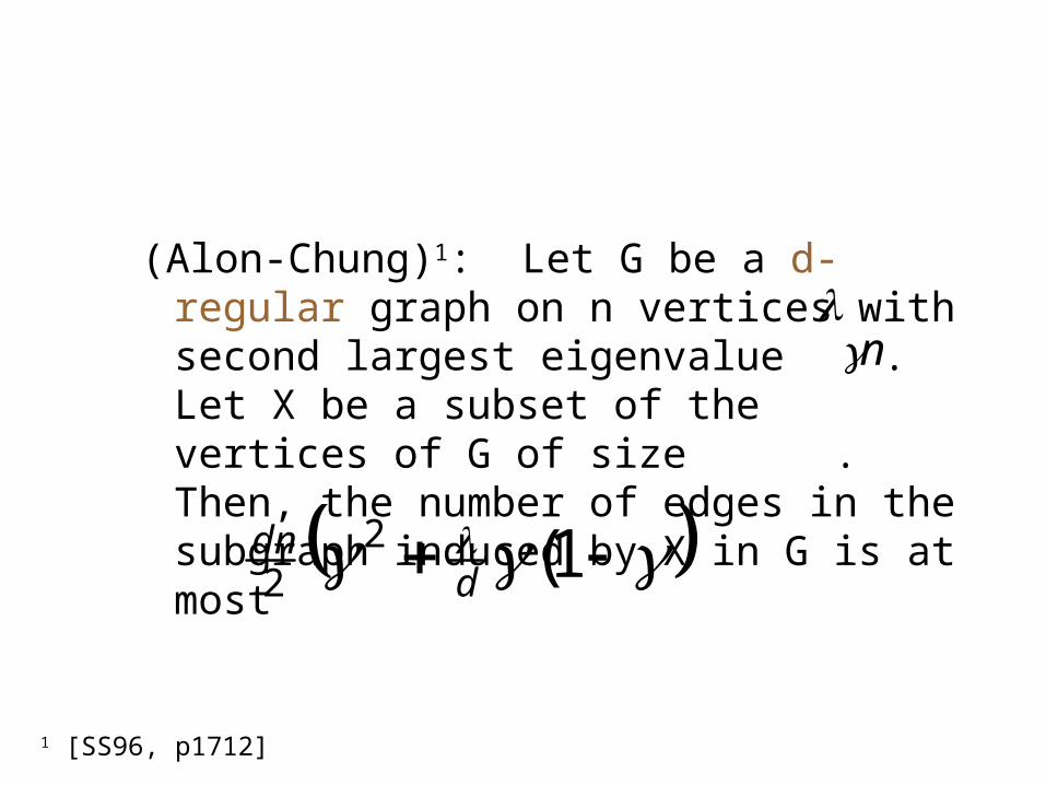
(Alon-Chung)1: Let G be a d-regular graph on n vertices with second largest eigenvalue . Let X be a subset of the vertices of G of size . Then, the number of edges in the subgraph induced by X in G is at most

1(22 d

dn

n

1 [SS96, p1712]

• Could use Alon-Chung bound to quantify the expansion factor of the edge-vertex incidence graph B(G)

• But a direct application of Alon-Chung itself works well in proof

• => each decoding round removes a constant fraction* of error from input words within threshold of nearest codeword. *(fraction <1 for

sufficiently large choices of block length d of S)

• => after O(log n) rounds, no error remains.

Circuit for Parallel Decoding1

• Each parallel decoding round can be implemented by a circuit of linear size and constant depth

– constraint satisfaction: constant # of layers of XOR’s

– variable “flips”: majority of constant # of inputs

• => Total of O(log n) rounds needs a circuit of size O(n log n), depth O(log n).

1 [SS96, p1715]

Linear Time of Sequential Simulation (Uniform Cost Model)

• During each round, compile a list of all constraints which might be unsatisfied at the beginning of next round by including:

– All constraints of previous round’s list which actually were unsatisfied

– All constraints neighboring at least one variable which received a “flip” message in current round

1. Total amount of work performed by algorithm is linear in the combined length of these lists:

– Each round: Check which constraints from input list are actually unsatisfied; do decodes on S; send “flips”

– Regularity, fixed code S => constant local cost

2. Total length of these lists is linear in block length n of the code C(B,S).

– # variable errors decreases by constant ratio each round – Only constraints containing these variables appear in lists– => convergent geometric series, first term O(n)

Linear Time of Sequential Simulation (Logarithmic Cost Model)

Challenge: • Need O(n) bit additions and O(n) memory accesses• Cost per access is O(log n)• Total cost O(n log n)Solution:• Retrieve an O(log n) byte per access, only need to make

O(n/log n) accesses; total cost O(n)• Encode each byte with a good linear error-correcting code• Algorithm will correct a constant fraction of error in

overall code unless there is a constant fraction of error in the encoding of a constant fraction of bytes.

Expander Codes Wrap-Up1

• Error distance from a correct codeword was corresponded to a potential1 (of unsatisfied constraints) in a graph whose expander and regularity properties guarantee the success of a linear-time decoding algorithm which steadily decreases this potential to zero.

• Quadratic time encoding / linear time decoding• Superior speed of sequential decoding on random

expanders• Can tune parallel decoding algorithm for better

performance1[SS96, p1718-20]

Expander Codes Wrap-Up

• Average-case error-correction results in experiments much better than bounds predict (worst-case).

• Introducing random errors in variable flips can further improve performance.

• For random expanders, degree 5 at variables seemed to give best results.

Linear-time Encodable/Decodable Error-Correcting Codes

• Expanders leveraged to produce linear time encodable/decodable error-reduction codes

• Construction involving a recursive assembly of smaller error-reduction & error-correcting codes gives linear time error-correcting codes.

• Decoding algorithm, proof of its correctness are the same flavor as those already encountered.

• Randomized / Explicit constructions– Explicit case shown here is a generalization of the

randomized one

Historical Context1

• Prior constructions did not always use such well-defined models of computation or deal with asymptotic complexity

• Juntesen and Sarwate used efficient implementation of polynomial GCD algorithm to get O(n log n log log n) encoding, O(n log2 n log log n) decoding for RS and Goppa codes.

• Gelfand, Dobrushin, and Pinsker gave randomized constructions for asymptotically good codes with O(n) encoding; but no polynomial-time algorithm for decoding is known.

1 [S96, p1723]

Main Theorem1

• There exists a polynomial-time constructible family of error-correcting codes of rate ¼ that have linear-time encoding algorithms and linear-time decoding algorithms for a constant fraction of error.

• The encoding can be performed by linear-size circuits of logarithmic depth and decoding can be performed by circuits of size O(n log n) and O(log n) depth, and can be simulated sequentially in linear time.

[S96, p1729]

Error-Reduction Codes

• Definition: A code C is an error-reduction code if there is an algorithm ER which, given an input word w with total # errors below threshold, can reduce the # of message bit errors in w to a constant fraction of the # of check bit errors originally present in w.– Note: for zero check bit errors, implies error-correction

of all errors in message bits.

• Can construct such codes from good expanders

Building the Error-Reduction Code: R(B,S)

• Necessary Ingredients– B a (c,d)-regular expander graph (c<d)– S a good block length d error-correcting code

with k message bits (rate = k/d)– A correspondence between the graph B and

the codewords of R(B,S).

variables (c-regular)

check bit clusters (d-regular)

cd

dcn

n

1v

nv

1C

dcnC

Corresponding

(c-regular) vertices (d-regular) vertices

message bits check bit clusters

),( SBRB

},,,{ 21 nvvv

dcn

},,,{ 21 dcnCCC

n

The error-reduction code R(B,S) 1

• The error-reduction code R(B,S) will have n message bits and (c/d)nk check bits.

• The n message bits are identified with the n c-regular vertices.

• A cluster Ci of k check bits is identified with each of the (c/d)n d-regular vertices.

• The check bits of cluster Ci are defined to be the check bits of that codeword in S which has the d neighbors of cluster Ci as its message bits

• R(B,S) can be encoded in linear time, (constant time for generating each check bit cluster; linear # of clusters)

1 [S96, p1726]

Parallel Error-Reduction round of R(B,S)1

(where is the minimum distance of S)

• In parallel, for each cluster, if the check bits in that cluster and the associated message bits are within relative distance of a codeword, then send a “flip” signal to every message bit that differs from the corresponding bit in the codeword.

• In parallel, every message bit that receives at least one “flip” message flips its value.

[S96,p1728]

6

Quality of an Error-Reduction Round on R(B,S)

• Take B as the edge-vertex incidence graph of a d-regular Ramanujan graph G

(Lubotsky et al: A dense family of good expander graphs)1

• Can show every error reduction round removes a constant fraction* of error from the message bits of input words which are within threshold of nearest codeword. *(fraction <1 for sufficiently large choices

of block length d of S)

1[S96, p1726]

Proof of Quality of Error-Reduction

• Analogous to that seen above for error-correction of explicitly constructed expander codes

• Relies on the same graph properties:– Regularity (and fixed code S)– theorem of Alon-Chung (~expansion)

Linear Time of Error-Reduction on R(B,S)

• Argument analogous to that for linear-time simulation of parallel error-correction for the explicitly constructed expander codes above

• For good enough eigenvalue separation (~expansion) of graph B & good enough min distance of code S, after O(log n) rounds, error in message bits will be reduced to within threshold required by recursive decoding of overall error-correcting code Ck.

Recursive Definition of the Error-Correcting Codes Ck

{Err-Red Rk}+{Err-Cor Ck-1} => Err-Cor Ck

2kR

kMkA kB kC

1kC

1kR

bits2 30

kn bits23 30

kn bits2 20

kn

bits2 20

kn

Recursive Definition of the Error-Correcting Codes Ck

To encode message :

• Use Rk-2 to encode

• Use Ck-1 to encode

• Use Rk-1 to encode

• Codeword of Ck:

kM kA

kB

kC

kA

)()( kkkk CBAM

kk BA

bits2 20

kn bits2 30

kn

bits23 30

kn

bits2 20

kn

bitscheck 23 20

kn bits message2 20

kn

bits2length block total 0knn

) (rate 41

kM

Linear-Time Decoding of codeword: • ER linear-time error-reduction for Rk

=> linear-time error-correction for Ck

– Proof by induction – Hypothesis: Assume linear-time decoding (error-

correcting) algorithm EC which works for all sub-codes Ci, i<k.

1. Run ERx on • Reduces error in

2. Run EC on • Corrects ALL errors in ! (by quality of ERx, I.H.)

3. Run ER0 on • Corrects ALL errors in !!! (by assumption on ER0)

)()( kkkk CBAM

kkk CBA )()( kk BA

kk BA )(kA

kk AM )(

kM

Remarks1

• By modifying this construction one can obtain asymptotically good linear-time encodable and decodable error-correcting codes of any constant rate r.

• Linear time codes of rate ¼ will correct about as many errors on average as expander codes of rate ½

1[S96 p1730-1]

Conclusions1. Graphs - interesting results obtained by choosing

clever correspondences for edges and vertices: E.g.

– Variables-Message bits / Constraints– Edges / Vertices of another graph– Alon’s generalization: correspond variables with all

length-k paths (here k = 2) in another graph

2. Probabilistic Method1

– A nice way of proving existence theorems. E.g. Suppose I can’t show or describe to you a particular object from a set S with property X, but perhaps I can prove that for an object randomly selected from S, Pr[X] > 0, ...

1http://www.math.uiuc.edu/~jozef/math475/description.pdf

Some questions to ponder…1

• Can rate vs. error correction tradeoffs be improved by a more natural (linear-time) decoding algorithm for these codes? (Present algorithm is an unnatural simulation of

a parallel algorithm) • Does there exist a (linear-time encodable?) code

for which a number of errors matching the Gilbert-Varshamov bound can be corrected in linear-time? How good can linear-time codes be?

1[S96 p1730-1]

References (1)

• Berlekamp, Elwyn R. Algebraic Coding Theory. Laguna Hills, CA: Aegean Park Press. 1984.

• Blahut, Richard E. Theory and Practice of Error-Control Codes. Reading, MA: Addison-Wesley Pub. Co. 1983.

• [LR00] Lafferty, John and Dan Rockmore. Codes and Iterative Decoding on Algebraic Expander Graphs. International Symposium on Information Theory and Its Applications. November 5-8, 2000.

References (2)

•[SS96] Sipser, Michael and Daniel A. Spielman. Expander Codes. IEEE Transactions on Information Theory, Vol. 42, No. 6, November 1996 p1710-1722•[S96] Spielman, Daniel A. Linear-Time Encodable and Decodable Error-Correcting Codes. Ibid. p1723-1731•Sudan, Madhu Lecture Notes from “Algorithmic Introduction to Coding Theory”. Fall 2001(2002) MIT.