LINEAR THERMODYNAMICS AND THE MECHANICS OF SOLIDS

The Thermodynamics of linear irreversible processes is presented from a unified

viewpoint. This provides a new and synthetic approach to the linear mechanics of

deformation of solids, which includes as particular cases the classical theory of

Elasticity, Thermoelasticity and Viscoelasticity. The first two sections constitute an

introduction to the general concepts and principles of linear Thermodynamics as

developed in the writer’s earlier work and presented in somewhat more detail. This is

followed by the application of the general thermodynamic theory to Thermoelasticity

which combines the theories of Elasticity, Heat Transfer, and their coupled effects

into a single treatment. Some immediate consequences are derived such as the property

of diffusion of entropy and certain fundamental relations with reference to thermal

stresses. The introduction of inertia forces leads to a general formulation of thermo-

elastic dissipation of dynamical systems by Lagrangian methods. The second order

heat produced by the dissipation is evaluated. Linear Viscoelasticity and Relaxation

Phenomena are also a particular case of the thermodynamic theory. The resulting

stress-strain relations with heredity properties are discussed. The operational

formulation of these relations leads naturally to a formal correspondence with the

theory of Elasticity and to an operational-variational principle. The latter provides a

generalization of Lagrange’s equations in integro-differential form to the dynamics and

stress analysis of viscoelastic structures. Some specific applications of these

principles are presented.

L

Introduction

In recent years new and remarkably fruitful concepts

and methods have been introduced in Thermodynamics

which lead to a phenomenological approach for irreversi-

ble phenomena. Th e major contribution was made by

Onsager in 1931 when he introduced his now famous

reciprocity relations. In the realm of linear phenomena

the treatment of thermodynamics can be made completely

systematic and general. Application of this general

thermodynamics is of considerable interest in the field of

linear mechanics of solids. In the course of a general

research program on the mechanical properties of rock we

developed a general f r o mulation of irreversible phenom-

ena which uses generalized coordinates and Lagrangian

concepts and is applicable to a very wide class of

Ph enomena. The th eor was subsequently applied to y

Viscoelasticity, Thermoelasticity and Heat Transfer and

the mechanics of porous media bringing these phenomena

within the scotue of a single more general theory. It also

provides a new foundation for the classical theory of

Elasticity.

We have attempted to present a perspective of this

development. Some new results are also included. We

have dwelt in somewhat more detail than in the original

M. A. Biot

Shell Development Company and Cornell

Aeronautical Laboratory Inc.

papers on the derivation of the basic thermodynamic

equations, which is the object of Sections 2 and 3. The

concept of hidden coordinates and the “black box” ap-

proach to a thermodynamic system lead directly to relaxa-

tion and heredity laws. The resulting expression for the

impedance matrix is readily applied to the stress-strain

relations of viscoelasticity as presented later in Section

6. The symbolism of the operational calculus has been

preferred since it is most convenient in applications.

The field of Thermoelasticity which is understood here

to include thermal stresses, thermoelastic damping and

heat transfer is treated in Secttons 4 and 5. It constitutes

an excellent subject for illustrating the new principles.

A general formulation of linear viscoelasticity, i.e. the

mechanics of materials which exhibit relaxation and

heredity effects, follows immediately from the general

thermodynamic theory, particularly from the expression

developed for the thermodynamic impedance. This is

discussed in Section 6 and special emphasis is put on

the specific features of the operators which depend on

thermodynamics. We conclude in Section 7 with applica-

tions to the stress analysis and dynamics of viscoelastic

structures and review some general properties which are

direct consequences of a correspondence rule and an

operational-variational principle.

1

Generalized Concepts of Free Energy and

Dissipation Function

We shall first introduce the conceptual and mathe-

matical foundation of the linear thermodynamics of ir-

reversible processes and elaborate somewhat beyond the

original presentation as developed in several earlier

papers [ll, El, f_31. Throughout the text we shall use the word thermo-

dynamics as referring to irreversible processes and

reserve the term thermostatics for the description of

equilibrium states.

Let us consider a thermodynamic system designated as

system I and whose thermodynamic state is defined by a

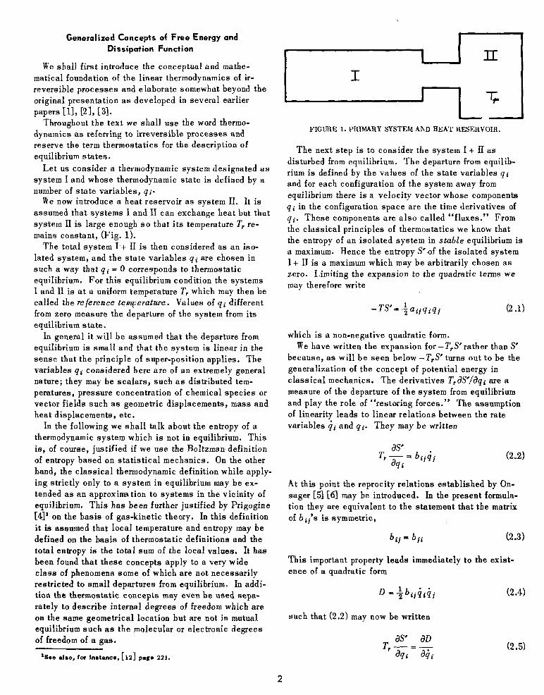
number of state variables, qi- We now introduce a heat reservoir as system II. It is

assumed that systems I and II can exchange heat but that

system II is large enough so that its temperature Tr re-

mains constant, (Fig. 1).

The total system I.+ II is then considered as an iso-

lated system, and the state variables qi are chosen in

such a way that qi = 0 corresponds to thermostatic

equilibrium. For th is equiIibrium condition the systems

I and II is at a uniform temperature T, which may then be

called the refereazce temperature. Values of qi different

from zero measure the departure of the system from its

equilibrium state.

In general it will be assumed that the departure from

equilibrium is small and that the system is linear in the

sense that the principle of super-position applies. The

variables qi considered here are of an extremely general

nature; they may be scalars, such as distributed tem-

peratures, pressure concentration of chemical species or

vector fields such as geometric displacements, mass and

heat displacements, etc.

In the following we shal1 taIk about the entropy of a

thermodynamic system which is not in equilibrium. This

is, of course, justified if we use the Boltzman definition

of entropy based on statistical mechanics, On the other

hand, the classical thermodynamic definition while apply

ing strictly only to a system in equilibrium may be ex-

tended as an approximation to systems in the vicinity of

equilibrium. Th’ h b is as een further justified by Prigogine

141’ on the basis of gas-kinetic theory. In this definition

it is assumed that Iocal temperature and entropy may be

defined on the basis of thermostatic definitions and the

total entropy is the total sum of the local values. It has

been found that these concepts apply to a very wide

class of phenomena some of which are not necessarily

restricted to small departures from equilibrium, In addi-

tion the thermostatic concepts may even be used sepa-

rately to describe internal degrees of freedom which are

on the same geometrical location but are not in mutual

equilibrium such as the moIecuIar or electronic degrees

of freedom of a gas.

I

. I T --

FIGURE 1. PRIMARY SYSTEM AND HEAT RESERVOIR.

The next step is to consider the system I + II as

disturbed from equilibrium. The departure from equilib-

rium is defined by the values of the state variables qi

and for each configuration of the system away from

equilibrium there is a velocity vector whose components

qi in the configuration space are the time derivatives of

qi. These components are also called “fluxes.” From

the classical principles of thermostatics we know that

the entropy of an isolated system in stable equilibrium is

a maximum. Hence the entropy S’of the isolated system

I + II is a maximum which may be arbitrarily chosen as

zero. Limiting the expansion to the quadratic terms we

may therefore write

(2 .l)

which is a non-negative quadratic form.

We have written the expansion for -TrS’rather than S

because, as will be seen below -T,s’turns out to be the

generalization of the concept of potential energy in

classical mechanics. The derivatives Z”rdS’/aqi are a

measure of the departure of the system from equilibrium

and pIay the roIe of “restoring forces.” The assumption

of linearity leads to linear relations between the rate

variables ii and qi. They may be written

as T r-== b *

aqi ijqj (2.2)

At this point the reprocity relations established by On-

sager [5] I_61 may b e introduced. In the present formula-

tion they are equivalent to the statement that the matrix

of bij’s is symmetric,

b bji ij = (2.3)

This important property leads immediately to the exist-

ence of a quadratic form

D P ~bij~irij

such that (2.2) may now be written

as ao Tr----=_

eqi aqi (2.5)

2

As pointed out above the function - T,S’ plays the same

role as the potential energy in the more restricted field

of mechanics. We put

(2.6)

and (2,5) become

av a0 -+-_a==0 aqi a4i

(2.7)

What is the significance of the function D? Multiplying

(2.5) by ii and adding we derive,

as dD Trx-,ii'2D

aqi (2.8)

In the process of returning to equilibrium the entropy S

of the isolated system cannot decrease, therefore

&‘/at 3 0 and D is a non-negative quadratic function of

the velocities Qi Equations (2.7) are identical with those

of a mechanical system composed of springs and dash-

pots. The function D is proportional to the rate of dis-

sipation of energy in the dashpots. The term dissipation

function is borrowed from mechanics to designate the

function D in the more general thermodynamic case.

Since W/& ,is the rate of production of entropy in the

system I + II the dissipation function is

D = f T, x (rate of entropy production) (2.9)

As regards the function V an important aspect of its

thermodynamic significance is added if we express the

entropy S’ of the system I + II in terms of the thermo-

dynamic functions of the system I alone. We may write

S’=S+S, (2.10)

where S is the entropy of system I and S, the entropy of

the heat reservoir II. Denoting by h the heat transferred

from system I to system II, conservation of energy re-

quires that

U h IE- (2.11)

where U is the internal energy of system I chosen so that

u = -h = 0 at equilibrium. The entropy SR of the reser-

voir II is also chosen to be zero at equilibrium, hence,

h U SR iE-----I_-

Tr Tr (2.12)

Substituting in (2,lO) we find

V = - T,s’z U - T,S (2.13)

We recognize here an expression which looks very much

like the free energy of classical thermodynamics. There

is, however, one difference in the fact that T, does not

refer to the temperature of system I but to the reference

temperature of the heat reservoir II. Expression (2,13) is

much more general than the classical free energy since

the system I may have an arbitrary distribution of non-

uniform temperature. Of course if the transformation is

isothermal and occurs at the temperature Tr itself, (2.13)

coincides with its classical definition. For want of a

better term we have referred to V as the generalized free

energy.

An alternate expressian for V which is of considerable

interest in applications was derived in [3]. We denote by

V,= U,- T,S, (2.14)

the classical value of the free energy corresponding to a

uniform temperature T, and by V, the amount by which V

increases when the initial temperature T, at any particu-

lar point is raised to T, + 8 i.e, when a non-uniform dis-

tribution of temperature increments 8 is imposed on the

system without changing the other state variables. We

may write

v = v, + v, (2.15)

and

vc = U, - TJ, (2J6)

or

(2.17)

vc =

The above expressions refer to the volume integral over

the volume r of system I and c is the specific heat per

unit volume for all variables constant except the tempera-

ture. For small variations 6 we may write

Hence

(2.18)

(2.19)

The term Vr represents the classical free energy for iso-

thermal transformations at the reference temperature T,

3

i.e. when T, represents the temperature of the system

itself instead of just that at the heat reservoir. It is the

Helmholtz free energy familiar to the physical chemist.

The additional term represents the thermodynamics of

power engineering i.e. the heat which may be transformed

into useful work. It can be seen that it is an integrated expression for the product of the heat cd0 by the Carnot

efficiency 0/( T, + 0) g O/T, Our expression (2.13) and

(2.19) may, therefore, be considered as a generalization

of the Helmholtz free energy to systems at non-uniform temperature.

With reference to Onsager’s relations we should point

out that theoretically they are valid only for systems

which exhibit microreversibility. In the presence of

magnetic and Coriolis fields of sufficient intensity they

are not applicable. Known examples of this are the Hall

effect for electrical conductivity and the Rhigi-Leduc

effect for thermal conductivity.

We should also bear in mind that the adjunction of the

heat reservoir II does not mean that there is necessarily

a heat exchange between I and II. This will depend on

the thermodynamic constraints and adiabatic transforma-

tions are therefore not excluded. However, the con-

straints must respect energy conservation. Further de-

velopment on the statistical foundations of the Onsager

relations were the object of more recent studies by On-

sager and Machlup [?I, Machlup and Onsager 181, Callen

Barasch and Jackson [9] and Greene and Callen [lo]. An

introduction to the subject will also be found in [ll] [I21

[131 and [141.

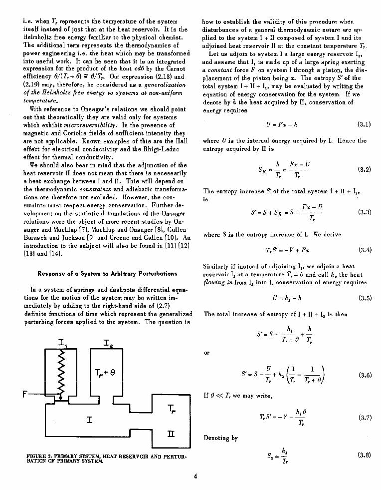
Response of a System to Arbitrary Perturbations

In a system of springs and dashpots differential equa-

tions for the motion of’the system may be written im-

mediately by adding to the right-hand side of (2.7)

definite functions of time which represent the generalized

perturbing forces applied to the system. The question is

FIGURE 2. PRIMARY SYSTEM, BEAT RESERVOIR AND PERTUR- BATION OF PRIMARY SYSTEM.

how to establish the validity of this procedure when

disturbances of a general thermodynamic nature are ap-

plied to the system I + II composed of system I and its

adjoined heat reservoir II at the constant temperature T,. Let us adjoin to system I a large energy reservoir I,,

and assume that I, is made up of a large spring exerting

a constant force F on system I through a piston, the dis-

placement of the piston being x. The entropy S’of the

total system I + II + I,, may be evaluated by writing the

equation of energy conservation for the system. If we

denote by h the heat acquired by II, conservation of

energy requires

U=Fx-h (3.1)

where U is the internal energy acquired by I, Hence the

entropy acquired by II is

h Fx-U

SR=?=p r T, (3.2)

The entropy increase S’of the total system I + II + I,,

is

Fr - 0 S=S+SR=S+--

T, (3.3)

where S is the entropy increase of I. We derive

T,S=-V+ Fx (3.4)

Similarly if instead of adjoining I,, we adjoin a heat

reservoir I, at a temperature T, + 8 and call h, the heat

floluing in from I, into I, conservation of energy requires

U=h,-h (3.5)

The total increase of entropy of I + II + I, is then

s’=s ha h -- +_

T, + 8 T,

or

S-S-;+h(;-&)

If 8 << T, we may write,

T,s’c - v+y r

Denoting by

(3.6)

(3.7)

(3.8)

4

the entropy inflow from I, into I we finally have

T,s’=- v+s,e (3.9)

We see that S, and 13 play the same role as the conjugate

coordinates F and x for the applied force. When the two

reservoirs I, and I, are added simultaneously the total

entropy S’of I + II + I, t I, is given by

T,s’=- V+Fx+S,O (3.10)

An alternate definition of the disturbing force is also ob-

tained by considering the expression (3.15) below. This

expression is quite general and if we add any number of

energy reservoirs disturbing the original system we may

write

TJ’= -V+Qiqi (3.11)

where Qi is an intensive quantity representing a force

and qi its conjugate extensive coordinate. As a further

example the force could be an electromotive force E and the quantity of electricity q flowing through the system

is then the conjugate coordinate leading to a term Eq in

expressions Qi qi. In the case of a chemical reaction the

mass M of constituent injected from a reservoir into a

particular phase or chemical species is the extensive

coordinate while the chemical potential P of this con-

stituent is the conjugate force. The corresponding term

in Qiqi is PM. The theory is therefore applicable to an

“open system.”

We may now apply the same reasoning as in the

previous section and assume that Onsager’s relations

apply to the total isolated system I + II + I, + I, + . . . Ii. We may then write as above (2.5),

(3.12)

Substituting (3.11) we derive

dV cYD -++-=Qi aqi %i

(3.13)

These equations are derived for constant Qi but they

obviously apply for arbitrary time variations of Qi since

the rates ii of all state variables must depend only on

the instantaneous configuration and forces.

Equations (3.13) are the fundamental equations for the

time history of the thermodynamic system, under the

external forces,Qi. We have derived them in less detail

in [l] and [21. In these same papers we also derived a

number of important properties which are straightforward

consequences of (3.13) and which we now briefly

describe.

The existence of normal coordinates follows from the

existence of the quadratic invariants V and D. Relaxa-

tion modes satisfying orthogonality relations are derived

from the corresponding eigenvalue problem. If the system

is in the vicinity of stable equilibrium V is positive

definite and all relaxation modes are proportional to an

exponential time decay. If the system is unstable (e.g.

under conditions of buckling) V is then indefinite and

there exist modes proportional to increasing exponentials.

The exponentials are always real because they corre-

spond to eigenvalues of two quadratic forms one of which,

D, is positive definite.

The dissipation function D is proportional to the

entropy production and we have shown [2] that the . instantaneous velocity vector qi of the system minimizes

the entropy production for all vectors satisfying the con-

dition that the power input of the disequilibrium forces

X,=yi_$ is constant i.e. if i

. Xiqi = const. (3.14)

An important expression is derived by considering a

system in equilibrium under the forces 0s”. We may

then write

and from the properties of quadratic forms

v = $qiQ!")

(3.15)

(3.16)

This expression is convenient in practical applications

to obtain V when relations such as (3.15) are known.

General expressions for the solutions of the funda-

mental equations in terms of the applied forces Qi as

given functions of time are easily obtained in operational

form [l]. We write

qi = A:iQj (3.17)

where ATj = ATi is a symmetric admittance operator

(s) C!P) ATj= ~ c 11

P +A, + Cij (3.18)

with p a time derivative operator

d P=z (3.19)

and X, are characteristic roots of the differential equa-

tions (3.13) changed in sign. For a stable system the

5

h, are real and non-negative. The diagonal coefficients

C$f’ and Cii are non-negative. The significance of the

operational expression is a multiple one*. In the case of

forces which are simple harmonic functions of time, say

Qiexp (iot) with a constant amplitude Qi, the amplitudes

qi of the response Qiexp (iat> are given by (3.18) after

putting p = io. Equations (3.18) may therefore be con-

sidered as relations between Fourier or Laplace trans-

forms of Qi ad qi. They may also be considered as

integral expressions when the forces are arbitrary func-

tions of time since we may write

*Qi(t) = e-‘st s

*eAs7dQi(r) (3.20) s 0

The reader’s attention is called to the advantages of

generality and flexibility attached to the use of the

operational notation throughout. Important relations of the impedance type are derived

if we introduce the concept of “hidden coordinates.”

The thermodynamic system is considered as a “black

box” with a large number of coordinates which are un-

observed qs. Perturbations (i.e. forces) are only applied

to observed coordinates qi while the forces applied to

the hidden coordinates qs are zero. A model for this is

a large resistance-capacity network with certain numbers

of outlet terminal pairs. We are interested in the rela-

tions between the applied forces Qi and the compounding

observed coordinates qi. This introduces the impedance

matrix of the thermodynamic system. We have shown

[l] that

Qi = Z*i qi (3.21)

where Z;j = ZTi is a symmetric impedance operator

(3.22)

The relaxation constants r, and all diagonal terms D$‘,

Dii, D:i are non-negative. Expressions (3.20) and (3.22)

are completely general and are valid whether the matrices

of the original differential equations are singular or not

or whether they have any number of multiple characteris-

tic roots. Attention is called to the fact that in the

derivation of (3.22), [l], we must invoke the non-negative

character of the dissipation function otherwise a term

in p* would appear in that expression.

A very useful variational principle equivalent to the

Lagrangian equations (3.13) is obtained by introducing

an operational form of the dissipation function

D* = ~pbijqiqj (3.23)

*For an introduction to operational methods see e.g. [IS], [161.

We may then write the variational principle as

SV + SD* = QiSqi (3.24)

This principle will be used later and also generalized in

Section 7.

Thermoelasticity

An excellent illustration of the new methods and

principles presented above is provided by their applica-

tion to Thermoelasticity as we have already pointed out

in [l] and [2] and developed more explicitly in the later

papers [3] and [I?].

It should be understood that the word Thermoelasticity

is used here in its broadest meaning and embraces as

particular cases the classical theory of Elasticity, the

effect of temperature distribution on thermal stresses in

elastic bodies, the theory of heat conduction and heat

transfer and the coupled interaction between the de-

formation and the temperature field which results in

thermoelastic damping.

The subject of Thermoelasticity has been the object

of well known discussions in the literature for over a

century among others by Duhamel [18], Neumann 1191 and

Voigt [20]. Duhamel’s equations which were reproduced

by Neumann are not based on thermodynamic principles

and are restricted to isotropy. They are based on the

experimentally known difference between the two specific

heats. Thermoelastic damping was studied extensively

both theoretically and experimentally by Zener 1211,

[221, 1231, 1241. Th e p resent treatment brings all these

phenomena into the general frame of linear thermody-

namics and its variational treatment as outlined above.

In addition it leads to new concepts and methods, in

particular to the concepts of thermoelastic potential, a

general dissipation function which includes surface

heat transfer, and a thermal force defined by a method of

virtual work in analogy with mechanics. Finally, as we

have shown in [17], which deals specifically with the

heat transfer aspects of the theory, the methods are

susceptible of considerable extension beyond the scope

of the present outline to include non-linear phenomena

and new procedures of numerical analysis.

The concept of thermoelastic potential which we have

proposed is entirely different from the expression used

by P&ler 1251 and which has been mistakenly referred to

as a thermoelastic potential. Not only is the expression

essentially different from ours, but the temperature plays

the singular role of a parameter not subject to variation

leading to a theory which does not contain heat transfer

processes in variational form and does not fit in the

scheme of the present general thermodynamic formulation.

The potential used by PIsler is expression (4.32) below

6

and referred to by Voigt [lo] as the first thermodynamic Withthe vector Sthe classical equations (4.1) may also

potential. be put in an equivalent form by writing

The classical equations for the coupled elastic and

thermal fields are

dopFrv

dx,= 0 (4.1)

aqLv -= 0 ax, k,. ?f= T as,

81 axi - r at

T*divS= -CO - TrBijeij

(4.5)

& kij $ = c z + T,pij 2

[ 1 i The stress tensor is Us,,, the strain is

1 dUi auj e..- -

( )

-+- “- 2 dXj C3Xi

(4.2)

and 6’ is the excess temperature above the reference

temperature T,.. The th ermal conductivity tensor is kij,

c is the specific heat per unit volume, for zero strain,

pij is related to the thermal dilatation properties of the

material, and C$ are the elastic moduli for isothermal

deformations (0 = 0). We have the following symmetry

properties

Cij = C~JJ = C:P= Ccv !-QJ II

pij = Pji

kij = kji

(4.3)

The latter is only true in the absence of a strong mag-

netic field or Coriolis forces, as a consequence of On-

sager’s relations. Experimental confirmation of the

symmetry of kij was found by Voigt [ll].

A rederivation of the classical equations (4.1) may be

found in the introductory part of 131 or in 1271.

Thermoelastic phenomena obviously must obey the

laws of linear thermodynamics. We have shown 131 that

they obey the general variational formulation represented

by the principle of minimum dissipation and the corre-

sponding Lagrangian equations (3.13).

In order to show this we must of course choose the variables which define the thermodynamic state of the

systems and correspond to the coordinates qi of the

general theory. The coordinate system chosen is the

field of displacement vectors uof the solid and in addi-

tion the vector field Sof entropy displacement. The

vector Sis the time integral of the rate of heat flow

divided by T,.. In this choice we are guided by expres-

sion (3.8). Hence,

where c@/dt is the

aS 1 an at=r,at

rate of heat flow.

(4.4)

The components of Sare designated by Si. The third

equation expresses the law of heat conduction while the

fourth is derived from the thermostatic definition of

entropy [3] assumed to be valid for non-equilibrium

phenomena following the assumptions of linear thermo-

dynamics (Section 2).

Let us evaluate the generalized free energy J’. Ac-

cording to (2.19) this may be written

1 v=vr+-

2 (4.6)

The isothermal free energy V is nothing but the well

known isothermal strain energy of the classical theory of

Elasticity.

where

w = lcii e

2 pu ijepv (4.8)

and C$ are the isothermal elastic moduli.

(4.9)

This is the particular form assumed by the generalized

free energy 131. S ince it embodies completely the thermo-

static and elastic properties of the systems we have

referred to expression (4.9) as the thermoelastic potential.

Substituting the value of 8 derived from (4.5) we express

this thermoelastic potential in terms of the fields cand

Sas follows.

v= + z(divS+ /3ijeii)2 dr 1 (4.10)

7

The dissipation function is easily found by using its

definition (2.9) in terms of entropy production. We found

131 [171,

;TrSS, f (%)‘dz4 (4.11)

In this expression the matrix of hi, is the thermal resis-

tivity matrix i.e. the inverse of the conductivity matrix

kij

[Xijl = [kij]”

The first integral is proportional to the entropy produc-

tion inside the system. The second integral taken over

the boundary A of the system corresponds to the entropy

production in the heat transfer layer at the boundary.

The heat transfer coefficient at the boundary is denoted by K and S, is the normal component of Sat the bound-

ary. We may also use the alternate operational definition

of the dissipation function following (3.23) and write

XijSiSjdr+ :Tr $dA (4.13)

Finally we must evaluate what corresponds to the

generalized virtual work QiSqi in the general variational

relation (3.24). This is the work performed on the sys-

tem by the “externally” applied forces and temperatures.

Here we must point out that while the force F is applied

to the solid boundary, the “external” temperature 8, is

that existing outside the heat transfer layer at the bound-

ary. The generalized virtual work is the surface integral

Qi8qi = (P*Sii+ O,SS,)dA (4.14)

where S, is the normal component of Sat the boundary

directed positively inwarP. The variational principle

corresponding to (3.24) is then

6V + 6D* = (F.&i+ 6,6S,) dA (4.15) A

where V is the thermoelastic potential (4.10) and o* the

operational dissipation function (4.13). This relation

must be verified for all variations of the fields cand

Sand as we have shown [3] [17] this leads to the classi-

cal equations in the form (4.5) for the thermoelastic

‘An additional term for body fuces may be ad&d as done in [3]. [Jf22 - MLM;;‘Md qs + Nis = Q, - M;,Mr,‘Qi (4.20)

field including the boundary conditions in the heat trans-

fer layer. Conversely, the variational principle (4.15)

also follows from (4.5). Hence if these equations are

taken to represent experimentally verified laws of elas-

ticity and heat conduction then the variational equution (4.15) is also true independently of the assumptions

peculiar to linear thermodynamics. In particular they

will be true without having to assume 8 << T,. This is

valuable in heat conduction when the methods and

principles then become applicable for variations of 6’

in a large range [l?].

The variational principle makes it possible to express

the thermoelastic equations for homogeneous or in-

homogeneous bodies, isotropic or anisotropic, in any

system of curvilinear or generalized coordinates. If we

use generalized coordinates qi we may describe the

fields uand Sin terms of fixed configurations iii and

5,. We write,

The set of generalized coordinates is qi and qS. As we

have shown 131 the differential equations for these co-

ordinates may then be written in the form (3.13) as

with partitioned matrices, Qi representing the mechanical

forces and QS the thermal forces (Mi, is the transpose of

M,J. We may restrict ourselves to applying a certain

number of mechanical forces Qi and observe the corre-

sponding coordinates qi (qs being “hidden”), all other

forces being zero. We may then write

Qi = -Gj qj

with a thermoelastic impedance

P D$y’ + Dij P + rs

(4.19)

This expression is a particular case of (3.22) and may be

derived by following the general procedure which we

used in [l]. They are a consequence of the particular

nature of the matrices in (4.17). In the derivation use

must be made of the fact that the generalized free energy

is non-negative.

An important property of thermoelastic systems is

derived from (4.17). Eliminating qi by matrix multiplica-

tion yields

8

Since the matrices multiplying qS and is are symmetric

this may be considered to represent a pure relaxation unit volume is the integrand in (4.9) i.e.

phenomenon for the entropy field. The entropy therefore 1 co2 T, obeys quite generally diffusion type equations. This (4.25)

may be verified directly in the case of a homogeneous

2, = rV + - -= rd/ + g (/!?ijeij - S)’

2 Tr

isotropic body. In th is case the stress-strain law is’ This may be written

oij = 2 PLeij + 6ij (Xe - /30) (4.21)

(e = Gijeij)

v = +Clijeij + +OS (4.26)

and the thermal conductivity is

kii = 6ii k

an expression identical in form with (3.16) of the general

theory. For adiabatic deformations we must put s = 0 and

the generalized free energy becomes (4.22)

We have shown [3] that the entropy per unit volume or

specific entropy or

s = -divs (4.23)

satisfies the diffusion equation

This means that if we suddenly deform an isotropic elas-

tic body the specific entropy does not initially vary in-

side. It remains constant until it has had time to change

by diffusion from the boundaries. It is interesting to in-

terpret this in terms of the analogy which we have demon-

strated to exist between thermoelasticity and the iso-

thermal mechanics of elastic porous media containing a

viscous compressible fluid 131. The specific entropy

plays the role of what we have called the fluid content

5 [28] [30]. When we suddenly form such a porous body

there is generally an instantaneous flow of the fluid but

there is at first no change in fluid content 6 inside the

body until it diffuses from the boundaries. Complete iso-

morphism exist between the two theories and the general

solutions of the equations of consolidation of porous

media of reference [28] apply to thermoelasticity and the

evaluation of thermal stresses by a simple change in

notation. The isomorphism is a consequence of the fact

that both phenomena obey the same basic thermodynamic

principles. It is of considerable interest to point out that for iso-

tropic bodies the thermal conductivity as expressed by

(4.22) automatically satisfies rhlsager’s relations purely

on the basis of geometric symmetry.

We shall add a remark concerning the significance of

the thermoelastic potential (4.9). Its specific value per

4h and P are the isothermal Lam; constants. From (4.28) the adiabatic La& constants are h + ,~‘T,/c and p.

T, V = W + c (pijeij)' (4.27)

1 e..e

81 w (4.28)

This represents the elastic strain energy for adiabatic

deformations and the expressions in the bracket are the

adiabatic elastic mod&. They are derived here very

simply from the generalized free energy. The same procedure may be used to derive the adiabatic com-

pliance coefficients. It is interesting to compare (4.26)

with the concept of thermodynamic potential which in

case the stress is a hydrostatic pressure p, is u - ST +

pe. Generalized to the stress tensor this is written5

(4.29)

In our notation with T = T, + 8 it becomes

(4.30)

Taking into account (2.13) and (4.26) we find

5=-v (4.31)

The quantity 5 is mentioned by Voigt [20] who refers to

it as the second thermodynamic potential. Although it

differs only in sign from our generalized free energy it is

a very different physical concept, which refers only to

isothermal properties at the temperature T = T, + 8.

Voigt also considers the classical isothermal free energy

t= 1 ce2

a-s(T,+O)=F’---- 2 T, @ijeij (4.32)

which he refers to as the first thermodynamic potential.

Expression (4.32) was used by PIsler [25].

5u is the internal energy per unit volume.

9

rated into two groups

= Qi

av a0 -+-y=o ah ah

multiplying the first equations by ii and the second by . q s and adding, we obtain

(5.13)

The right hand side represents the power input of the

mechanical forces. On the left the term 2 D equal to

twice the dissipation function is non-negative and

represents the irreversible conversion of mechanical

power into heat. This dissipation function D is given

by (4.11). This heat g eneration produced by the dissipa-

tion is a quantity of the second order which in a first

order theory is neglected in comparison with the first

order entropy flow vector Sas defined above. Over a

certain period of time this second order heat may of

course accumulate and if not diffused out will produce

an increase of temperature comparable to first order

effects. A direct verification of the conversion of the

dissipated power into heat is obtained by writing the first

law of thermodynamics in the form

dh du deii -- dt = - z + oij 7 (5.14)

dh where - -

dt is the heat exuded per unit volume and unit

time and u is the internal energy per unit volume. Re-

placing oPLv by its expression from the equation of state

i.e. the first equation (4.5); further, using the last

equation (4.5) and introducing the value, v from (4.26) we

find,

dh d -- dt =-dt

(u- (5.15)

The irreversible part of the power is obviously con-

tained in the second term. A simple calculation gives

the volume integral of this second term as

JJJT(9div ($jdr = 20 (5.16)

where D is given by (4.11). In order to establish this

last relation we integrate by parts and introduce the as-

sumption that the externally applied temperature 8, is

zero (Q, = 0). H ence in that case 2 D represents the

total heat exuded irreversibly from the volume.

Viscoelasticity

Viscous and relaxation phenomena in the linear range

may in general be assumed to obey the thermodynamic

equations formulated above. Strictly speaking of course

we must deal with a system which is initially in equilib-

rium and undergoing small disturbances from this state.

Actually we may expect the equations in certain specific

cases to be verified in a much wider range while in some

other instances non-linearities will appear even for

physically very small disturbances. Furthermore be-

cause of their wide validity the thermodynamic principles

lead to expression which in many cases give a first . .

approximation to the physical properties in the same

sense that Hooke’s law in Elasticity yields a widely

valid approximation to the actual properties of materials.

In this connection and as already pointed out in Section

1 we should remember that linearity does not insure the

validity of Onsager’s relations as they do not neces-

sarily apply in the presence of a magnetic field or a

field of Coriolis forces. However, in practice the actual

restrictions of this type to the validity of the equations

will appear only in exceptional cases.

Application of Onsager’s relations to viscoelasticity

were made by Staverman and Schwarzl 1321 [33] and

Meixner [Ml [35I. Simultaneously a very general ap-

proach to viscoelasticity based on linear thermodynamics

as presented here was developed by this writer [ll [2].

Our treatment appears to be more general since, as

illustrated in the case of thermoelasticity (Section 4), it

includes heat conduction as a particular case and the

coupling of thermomechanical effects with physico-

chemical, electrical, and other thermodynamic degrees of

freedom”. We also derived the general form of the

operational moduli relating stress and strain and made it

the object of a rigorous proof El]. We subsequently in-

cluded the treatment of a fluid-saturated porous visco-

elastic anisotropic solids 1361, and the application to the

dynamics of viscoelastic structures of some variational

principles which we had developed earlier for linear

thermodynamics [2]. This leads to a vuriational-

operational method and to Lagrangian equations with

operational coefficients [37] [38].

The operational relations between stress and strain

are an immediate consequence of expressions (3.17) and

(3.21). Consider an element of solid of unit volume.

The nine stress components oPLLYmay be identified with

the nine applied forces Qi to the system and the nine

components eij of the strain tensor are the corresponding

‘%t includes for instance a. a partlculpr case the theory of therm.1 stresses of viscoclastlc media with temperature independent atress- strain relations. This is formally ldentlcal with the treatment of paroua viscoelnstlc media [36].

11

observed coordinates qi. The solid is assumed to con-

tain hidden coordinates which may be finite or infinite in

number. The strain is then expressed in terms of the

stress by an operational compliance matrix A*,$ which

corresponds to the general admittance (3.18).

Solving the system for cr:i brings out operational moduli

which correspond to the impedance (3.22).

The operators are

pii _ s Oa c;v A) dx + c,,

pv- ~ I’

0 P+X

(6.2)

(6.3)

s 00

Z*ii= W LD;,,(r) dr + D$, + pD,$ (6.4)

0 p+r

The summations in expressions (3.18) and (3.22) are

replaced by integrals. This of course is more convenient

as an approximation if there are a great number of hidden

coordinates. In doing so we must take care of the fact

that C?,,(h) and D&,(r) may be highly discontinuous

functions. These discontinuities are due to the fact that

these functions include a spectral density factor for the

relaxation constants X and r and also because the co-

efficients Csj and DiT’ themselves in expressions (S)

(3.13) and (3.22) may be d iscontinuous functions of X,

and rS. The discontinuities may be of the Dirac function

type. The discreet spectrum in expressions (3.18) (3.22)

is included in the integral representations (6.3) (6.4) by

the introduction of Dirac functions. Further properties

of the operators (6.3) and (6.4) are

1. The operators satisfy the symmetry properties

A*ij_A*ij_A*ji PV VP - w

z* ij _ z* ij = z* ji PV - VP PV

which are consequence of the symmetry of oii and eij

2. In addition they satisfy the symmetry property

(6.5)

A* ii = A*PV pv il

(6.6) z*ii = Z*pV

pv 81

which is a consequence of the Onsager reciprocity

relations.

3. The variables X and rare real and non-negative.

They are real because of Onsager’s relations and the

non-negative diseipation functions D. They are non-

negative because we have assumed the system to be

disturbed in the vicinity of stable equilibrium, hence such that the generalized free energy V is non-negative.

4. All diagonal terms C!{(x), C$, and D:;(r), D$, 0:;’

are non-negative. This is also a consequence of On-

sager’s relations and the non-negative character of the

generalized free energy and the dissipation function.

This non-negative character of the diagonal terms is an

invariant property which must be valid for all linear

transformations of the six independent variables eij.

It follows that the coefficients C and D must be such . . . . that D&(r) eijepv, D&eiie&,$eije~v, C&((h) eijepv,

and C& eij epv are all non-negative quadratic forms.

As already mentioned above (Section 3), a more subtle

point in deriving expression Z>z is that from a purely

algebraic viewpoint there arises the possibility of an

additional term DLi’ pa which would introduce a depend-

ence on the strain acceleration. However, because we

are dealing with a positive-definite dissipation function

we were able to show [ll that the term in p* must vanish.

This point is an important one and although it was intro-

duced explicitly in [l] it was not given due emphasis.

We have assumed implicitly that the thermodynamic

equations involve the hidden coordinates only in V and

D. If this is not the case, i.e. if hidden coordinates

appear also in the kinetic energy we still derive the

symmetry properties 1 and 2 but the nature of the opera-

tors is affected by the possible introduction of complex

conjugate quantities. This will also affect the nature

of the heredity functions below (6.8)

We have written the above relations as operational

equations. The reader is reminded of the significance

of these equations. They may be considered as direct

relations between the Laplace transforms of the time

dependent functions. We may also introduce explicitly

differential and integral operation represented by the

operators in accordance with expressions (3.19) and

(3.20). Hence the stress-strain relations (6.2) may be

written as,

upv = s ‘h$(t - r) deij(r) + D$ + D;L 2 (6.7) 0

with an heredity tensor

h:,,(t) = Do Dzv(r) emrt dr. (6.8)

The function D:,,(r) is a “spectral tensor” of the

fourth rank. In this sense the spectrum depends on the

particular choice of the coordinate system for represent- ing the stress and the strain and on the particular con-

straints imposed on the system. We may manipulate (6.1)

or (6.2) as if the coefficients were algebraic quantities

12

and thus obtain the matrix relating any choice of stress

components with the corresponding strain. The new operators of course are not obtained in the form (6.4).

But it should always be possible to do so. If we call B(P) that part of the new operators which corresponds to

the integrals in (6.3) and (6.4), the problem amounts to

finding a function F(r) which satisfies the integral

equation

B(p) = Cm PF(r)dr. Jo P-fr

(6.9)

A very simple solution for this integral equation was

given by Fuoss and Kirkwood [39] in connection with

problems of dielectric relaxation of polymers. A discus-

sion of this integral equation in connection with one

dimensional problems of viscoelasticity has been given

by Gross 1401. Th e integral equation may be considered nf Pl-l,,F.&?P 5aa I lT,x”Pl.PI;Ic.t;,m nf .D” epn”“Gn” :” r.o.401 "Z ""..."I Y" Y ~"""'U"'U~'"Y "I uu ~CAUU'YL. 1nl pnlAcu

fractions. Once we know F(r) the operator B(p) may be

expressed immediately in terms of an heredity operator

by following the procedure outlined above. We may write

and the “operational Young’s modulus” is

F(r) dr + D + D> (6.14)

These relations show that the material is represented

by a model of springs and dashpots. Equations (6.12)

and (6.13) correspond to two equivalent models which are

respectively a Voigt model (Fig. 3) and a Maxwell model

(Fig. 4). We can see that the possibility of representing ,bP mnt,M.:al br m..-1. -a-lz.l” * CL*” .L_bb1LcaL “J ou\ru uvucj~u i8 63 CGiIS~pii~iIC~ Of the

Onsager relations and the non-negative character of the

generalized free energy and the dissipation function.

It is of interest to point out how thermodynamics

restricts the nature of the general type of operators which

would otherwise result from a purely mathematical ap-

proach to linear theory. A general linear relation be-

tween stress and strain would read

d where p = - is again the time derivative. We could

dt

B(p) = s 'h(t - r)d solve the system for opv and obtain a relation of the

0 form

with

h(t) = s O” F(r) e-"dr 0

(6.16)

(6.10) where the elements of the matrix P*ij polynomials in p. Expanding these

sly are quotients of algebraic functions

As an example we can use this method to derive the moduli Z* ‘ifrom the compliance matrix A$and vice

pu versa. One matrix is the inverse of the other

we shall obtain expression which are in general quite

different from (6.4) because

1. The roots I of the denominator may be complex

conjugates.

r7*iii _ rd*iil-l L-l$LyJ - L‘-pLV J

2. There may be terms in the expression of the type

(6 I?) . l/(P + r)” due to multiple roots.

3. The matrix is not in general symmetric except for

isotropic media.

Then any term of the inverse matrix may be written in

the form (6.4) by first separating the terms D$, + PD’~~ then representing the remainder in the spectral form i;

solving an integral equation of the type (6.9).

In the one dimensional case corresponding to a simple

tension test the stress o and the strain e are related by

either

e=A”o

o=Z*e (6.12)

where the compliance operator is

A* = rw E(X)

J -----a+C

0 P+x (6.13)

4. The diagonal terms may be negative.

5. Acceleration terms and higher order derivatives may

be present.

For a thermodynamic system as we have already

pointed out complex conjugate quantities may arise only

if there are hidden coordinates with kinetic energy.

We have pointed out iii isj that an important conse-

quence of the symmetry properties of the operational moduli is that they may be manipulated algebraically as

elastic moduli. This estabIishes a rule by which the

great generality of the equations of the classical theory

of Elasticity may be immediately extended to Visco-

elasticity by simply replacing the elastic moduli by their

corresponding operators. We have also shown 121 1371

1381 that the property extends to the variational and

energy methods replacing the strain invariants of the

theory of Elasticity by their corresponding operational

13

expressions. W e h ave referred to this as the corre- spondence rule. An immediate application of this rule

refers to properties of geometric symmetry [l]. An iso-

tropic material will be characterized by two operators,

cubic symmetry by three operators, transverse isotropy

by five operators, and so on. We have pointed out that

the frequency dependence of the operators leads to a

property which does not occur in the theory of Elasticity

i.e. that a material may change porn one type ofsym-

metry to another depending on the frequency range

considered.

In general this correspondence rule is a consequence

of the Onsager relations. However for an isotropic material this is not necessary since the geometric sym-

metry in this case insures the symmetry of the matrix of

the moduli. The stress-strain relations in this case are

aij = 2 Q* eii + ZiiiR* e

(e = Giieii)

with two distinct operators

Q(r) dr + Q + PQ’

R*= O” s ’ -R(r)dr+R+pR’ 0 P+r

(6.17)

(6.181

corresponding to the Lam& constants ,a and X. However,

the particular form above of the operators Q* and R* are

a consequence of thermodynamics and not of the iso-

tropy. A restricted form of correspondence has been known

for the incompressible isotropic case (41) (42) and has

been referred to sometimes as the “viscoelastic

analogy.” The general correspondence rule in the context of thermodynamics for both isotropic and aniso-

tropic media was first formulated by this writer [l]. For

the isotropic case it is clearly independent of Onsager’s

relations since geometric symmetry alone implies that

the compliance matrix is diagonal. We further developed

its corrollary, an operational-variational principle and other applications [37] [38] (see Section 7). We have

also extended the correspondence rule to isotropic and

anisotropic porous viscoelastic media [36]. In this case

Onsager’s relations are required even in the isotropic

case.

I

I I I

1

I 6

F'IGURE4.MAXWFaLLMODELOFVISCOELkSTICITY.

As mentioned above the term Viscoelasticity is used

here in a very broad sense to include all viscous and

relaxation phenomena including thermoelasticity. One

might ask, therefore, how the operational stress-strain

relations (6.1) (6.2) written above are related to the

treatment of Thermoelasticity in Sections 4 and 5. The

difference lies in the fact that in the present Section we

have considered the strain to be the only relevant ob- CI PPVP rl coordinate of the materia! element* “__ ..,- The stress-

strain relations (6.1) (6.2) are valid for Thermoelasticity

and correspond to hidden coordinates which represent

thermal changes inside an inhomogeneous polycrystalline

material. Other hidden degrees of freedom would be

represented for instance by viscous slip at intergrain

boundaries or by the phenomenon of solution and re-

crystallization due to local stresses and the correspond-

ing associated diffusion process.

Dynamics and Stress Analysis of Viscoelastic Structures

For “small” oscillations it may be expected that many

engineering structures obey linear viscoelastic laws.

This has been observed not only in continuous solids but

also in riveted structures such as bridges and aircraft

frames. Recent vibration tests of granular materials by

Duffy and Mindlin [43] 1 a so indicate properties closer to

a linear relaxation process rather than a Coulomb type

friction. The dynamics and stress analysis of viscoelastic

structures may be conveniently carried out by using

generalized coordinates. As we have shown 121 1191 [ZOI

an important aspect of the correspondence rule is the

possibility of introducing an operational-variational

method. We mean by this the use of a variational method on invariants with onPFatinna1 rnPffiriPntQ_ lr--------l- -__-- * _-_-_ “I. The n”PPa- -r--- tional invariant which corresponds to the elastic strain

energy is

Z:~epveii dr (7.1)

to Lagrangian equations in operational form

-t- T*) = Qi

Explicitly the equations are

( YTi + pzmij) qj = Qi

(7.4)

(7.5)

In general the theorem of Fuoss and Kirkwood will be applicable leading to a spectral representation of the

operator as

- YTj = s -!- Fij(r) dr + Yi j + Y;j p (7.6) () P+r

This operator is equivalent to the integro-differentiai

operations

YTj Qj = s thij(‘- r) dqj(‘) + Yij + Y:j ~ (7.7) 0

with the heredity functions

hii = s

m emrtFij(r)dr

0

(7.8)

Equations (7.5) therefore represent a generalization of

Lagrange’s equations to integro-differential form.

The function hii will be of the form (7.8) if On-

sager’s relations are applicable but it may also be of a

more general form since the operator is defined as La-

place transforms independently of any thermodynamics.

Furthermore the variational method above is valid for

isotropic media and in that case is also not dependent

on thermodynamics.

An interesting case in the dynamics of structures is

when the operators Zy: may be written,

The invariant corresponding to the kinetic energy has

already been introduced above as Z*ii = cFvf*

PV (7.9)

l 10-c T*L= --P JJJ /+& (7 2) where f* is an invariant operator and Cf!,,are constants

. which may depend on the location. We K&e referred to

this as the case of an homogeneous spectrum [38]. In

As we have shown [2] [37] [38], if we represent the de- this case the invariant J* becomes

formation field by generalized coordinates qi we obtain

the equations for qi by writing the variational principle _I* = ff* C$e,,eijdr (7.10)

&I* + ST* = Qisqi (7.3) 7

A where t-he right--hand side represents the virtuai work of With normai coordinates qi the two quadratic forms ap-

all forces applied externally to the system. This leads pearing in J* and T * may be reduced to a sum of squares

15

i.e. we may write

.I* = $f*dq;

T* = +p’q;

and the operational Lagrangian equations reduce to

independent equations

(7.11)

(7.12)

We have referred to such modes as partial modes 1371.

They may be calculated by the same method as in the

usual vibration analysis of elastic structures. All modes

have the same relaxation spectrum.

The same property- extends to cases where the ma-

terials are not necessarily represented by operators of

the type (7.9). Actually it is sufficient that for some

reason the invariant J* contain a single operator co- efficient. Such is the case for instance for an isotropic

incompressible material. In this case variations must be

constrained by the condition of incompressibility. More-

over, if there are boundary constraints they must be such

that no work is done, i.e. they are either free of stress or

have no displacement. In general this will be accom- -11-L-3 tt rr._ J_f__-_L:__ I_ ____r__:__Xl :_ _.._1. ^ _..^_. pllsueu ‘I Lilt: Uel”cL~aLI”II 1s ~“UJLLaIIIeU 11‘ JULll a war

that a single operator may be factorized. Such is the case for instance in the bending of a thin rod with end

conditions either clamped, pinned, or free. The invariant

J* in that case contains only a single operator E*. We

write

(7.13)

where w is the deflection of the rod as a function of the

coordinate x and I the cross-section moment of inertia.

The operator E * is obtained from the expression of

Young’s modulus in terms of the Lam& constants and re- ., placing the latter by R*

correspondence rule.

We find

E* =

and Q* in accordance with the

O*(.?R* -c ~.ti\ c \--- . -x ,

Q* + R* (7.14)

We may, therefore, analyze the bending vibrations of

such a viscoelastic rod by the use of normal coordinates

and for ends which are free, clamped, or pinned. The

same separation in normal coordinates may of course be

accomplished if the structure is composed of elements of

homogeneous material in which a rod type bending and

elongation is the predominant deformation.

If we neglect the inertia forces a structure composed

of an isotropic material may be analyzed by normal co-

ordinates since the invariant is separated into two terms

each multiplied by a different operator.

I* = ~JJJ[2Q* eijeij + R* e’]dr (7.15)

This constitutes the generalization of a procedure

suggested by Cosserat about sixty years ago for elastic

systems [441.

We shall end with a short remark on the nature of solid

friction. In problems of flutter analysis of aircraft struc-

tures it has been customary to take care of the solid

friction by replacing the rigidity moduli by complex

frequency-independent quantities. This may be approxi-

mated in the above representation if we put

Fij(r) = yijlr r > E

Fij(r) = 0 r<c

Expression (7.6) then becomes (with p = id

yzj = Iw --?.- z dr + Yij

6 io+r r

(7.16)

(7.17)

For a small value of 6 and y . the complex Yz is almost

constant for a wide range of “f requency.

The correspondence rule and the operational-variationa

principle are applicable to a very wide category of

practical problems. We have shown in [37] and [38] how

they lead to general methods in problems of dynamics

and stress analysis of viscoelastic plates and shells

even in non-linear problems of finite deflections.

In problems of thermal stresses in elastic and visco-

elastic structures, applications of the principles de-

veloped above has led to new concepts and methods. We have shown that a direct calculation of thermal stresses

is possible which avoids the necessity of first Cal&at-

ing the temperature field [45I.. The analysis can be

carried out entirely by variational procedures.

Acknowledgements

This work was sponsored jointly by the Shell Develop-

ment Company and the Cornell Aeronautical Laboratory.

Sections 2 and 3 are based on lectures delivered by this ..__tr__ ̂ & rL_ lT__......:11_ T _I.,,,+,.“., ,F dp ch,ii n,.,,i,,_ WTILtX aI. l.llt: KJlUe;1J,YLlle UL1”“LcU.“IJ “I L.fiICi U‘iGll YU “U’L”Y

ment Co. in February 1955.

16

Bibliography

I. Biot, M. A., “Theory of Stress-Strain Relations in

Anisotropic Viscoelasticity and Relaxation Phenomena,”

Jour. Applied Phys., Vol. 25, No. 11, pp. 1385-1391,

1954. 2. Biot, M. A., “Variational Principles in Irreversible

’ Thermodynamics with Application to Viscoelasticity,”

Phys. Rev., Vol. 97, No. 6, pp. 1463-1469, 1955. 3. Biot, M. A., “Thermoelasticity and Irreversible

m I nermodyiiamics, 11 r--._ A~_ IT-1 nt_.- 1, 1 JOW. qqwea rnys., VOL. 27, NO. 3,

pp. 240-253, 1956.

4. Prigogine, I., “Le Domaine de Validiti de la

Thermodynamique des Phdnome&es Irrkversibles,”

Physica 15, No. l-2, pp. 272-289, 1949.

5. Onsager, L., “Reciprocal Relations in Irreversible

Processes I,” Phys. Rev., Vol. 37, No. 4, pp. 405-426,

1931.

6. Onsager, L., “Reciprocal Relations in Irreversible

Processes II,” Phys. Rev., Vol. 38, No. 12, pp. 2265-

2279, 1931. 7. Onsager, L. and Machlup, S., “Fluctuations and

Irreversible Processes,” Phys. Rev., Vol. 91, No. 6,

pp. 1505-1512, 1953.

8. Machlup, S. and Onsager, L., “Fluctuations and

Irreversible Processes II,” Phys. Rev., Vol. 91, No. 6,

pp. 1512-1515, 1953.

9. Callen, H. B., Barasch, M. L. .and Jackson, J. L.,

“Statistical Mechanics of Irreversibility,” Phys. Rev.,

Vol. 88, No. 6, pp. 1382-1386, 1952.

10. Greene, R. F. and Callen, H. B., “On a Theorem

of Irreversible Thermodynamics II,” Phys. Rev., Vol. 88,

No. 6, pp. 1387-1391,1952,

11. Prigogine, I., “Etude Thermodynamique des

Phenomenes Irreversibles,” Desoer, Lidge, 1947.

12. De Groot, S. R., “Thermodynamics of Irreversible

Processes,” lnterscience Publishers, Inc., New York,

1952.

13. Prigogine, I., “Introduction to the Thermodynamics

of Irreversible Processes,” Charles C. Thomas, Spring-

field, Ill., 1955.

14. Denbigh, K. A., “The Thermodynamics of the

Steady State ,” Methuen’s Monographs, John Wiley, New

York, 1951.

15. von Karman, Th. and Biot, M. A., “Mathematical

Methods in Engineering,” McGraw-Hill Book Co., Inc.,

New York, 1940.

16. Jeffreys, H. and B. S., “Methods of Mathematical

Physics,” Cambridge Univ. Press, 1950.

17. Biot: M, A.; “New Methods in Heat Flow Analysis

with Application to Flight Structures,” Jour. Aeronauti-

cal Sciences, Vol. 24, No. 12, pp. 857-873, 1957.

18. Duhamel, J. M. C., “Second MCmoire sur les

Phdnomdnes ThermomCcaniques,” J. de Z’EcoZe Poly-

technique, 25, 15, pp. l-57, 1837.

19. Neumann, F. E., “Vorlesungen fiber die Theorie

der Elasticitlt der Festen K&per und des Lichtgthers,” B. G. Teubner, Leipzig, 1885.

20. Voigt, W., “Lehrbuch der Kristall Physik,” B. G.

Teubner, Leipzig, 1910.

21. Zener, C., “Internal Friction in Solids I,” Phys.

Rev., 52, pp. 230-235, 1937.

22. Zener, C., “Internal Friction in Solids II,” Phys.

Rev., 53, pp. 90-99, 1938. 23. Zener, C., Otis, W., Nuckolls, R., “Internal

Friction in Solids iii,” Picys. iiev., 53, pp. 100-101,

1938.

24. Zener, C., “Elasticity and Anelasticity of Metals,”

The University of Chicago Press, Chicago, 1948.

25. Pcsler, M., “Theorie der Thermische Dampfung in Festen K&per,” Zeit. f. Phys., Vol. 122, pp. 347-3&-j,

1944.

26. Voigt, W., “Gottingen Nachrichten,” 87, 1903.

27. Mason, W. P., “Piezoelectric Crystals and their

Application to Ultrasonics,” D. Van Nostrand, New

York, 1950 (Chapter 3 and Appendix).

28. Biot, M. A., “General Solutions of the Equations

of Elasticity and Consolidation for a Porous Material,”

Jour. Appl. Mech., Vol. 23, No. 1, pp. 91-96, 1956.

29. Biot, M. A. and Willis, D. G., “The Elastic Co-

efficients of the Theory of Consolidation,” Jour. Appl.

Mech., Vol. 24, No. 4, pp. 594-601, 1957.

30. Biot, M. A., “Theory of Propagation of Elastic

Waves in a Fluid-Saturated Porous Solid I. Low Fre-

quency Range,” Jour. Acous. Sot. Am., Vol. 28, No. 2,

pp. 168-178, 1956.

31. Rocard, Y., “Propagation et Absorption du Son,”

Hermann, Paris, 1935.

32. Staverman, A. J. and Schwarzl, F., “Non-Equi-

librium Thermodynamics of Viscoelastic Behavior,”

Proceedings Roy. Aca. Sci., Amsterdam, B. 55, No. 5,

pp. 474-490, 1952. 33, Staverman; A, J,, “Thermodvnamics of Linear

Viscoelastic Behavior,” Proc. Second lnt. Congress on

Rheology, pp. 134-138, Academic Press, New York,

1954.

34. Meixner, J., “Die Thermodynamische Theorie der

Relaxationserscheimnngen nnd ihr Zusammenhang mit

der Nachwirkungstheorie,” Kolloid Zeitschrift 134, 1,

pp. 2-16, 1953.

35. Meixner, J., “Thermodynamische Theorie der

Elastischen Relaxation” Zeitschrift fuer Naturforschung,

oa, 718, pp. 654-665, 1954.

36. Biot, M. A., “Theory of Deformation of a Porous

Viscoelastic Anisotropic Solid,” Jour. Appt. Phys.,

V0i. 27, NO. 5, pp. 459-467, 1956.

37. Riot, M. A., “Dynamics of Viscoelastic Aniso-

tropic Media,” Proceedings of the Second Midwestern

Conference on Solid Mechanics, Research Series No. 129,

Engineering Experiment Station, Purdue University,

Lafayette, Ind., pp. 94-108, 1955.

17

38. Biot, M. A., “Variational and Lagrangian Methods

in Viscoelasticity,” Deformation and Flow of Solids,

IUTAM Colloquium, Madrid, 1955, pp. 251-263, Springer,

Berlin, 1956.

39. FUOSS, R. M. and Kirkwood, J. G., “Electrical

Properties of Solids VIII. Dipole Moments in Polyvinyl

Chloride-Diphenyl Systems,” Jour. Amer. Chem. Sot.

* vol. 63, pp. 385-394, 1941.

40. Gross, B., “Mathematical Structures of the

Theories of Viscoelasticity,” Hermann, Paris, 1953.

41. Frenkel, J., “Kinetic Theory of Liquids,” Dover

Publications, Inc., 1955 (Translated from the original

Russian edition Moscow, 1943).

42. Alfrey, T., “Non-Homogeneous Stress in Visco elastic Media,” Quart. Appl. Math., Vol. 2, No. 2, 1944.

43. Duffy, J. and Mindlin, R. D., “Stress-Strain Re-

lations of a Granular Medium,” Jour. Appl. Mech., Vol.

24, No. 4, pp. 585-593, 1957.

44. Handbuch der Physik (ed. H. Geiger and K.

Scheel) Springer, Berlin, 1928, Vol. VI, p. 128 (Cos-

serat functions).

45. Biot, M. A., “New Thermomechanical Reciprocity

Relations with Application to Thermal Stress Analysis”

CornelI Aero. Lab. Report. June 1958 (to be

published).

18