Linear theory and measurements of electron oscillations in an inertial Alfv�enwave

J. W. R. Schroeder,1,a) F. Skiff,1 G. G. Howes,1 C. A. Kletzing,1 T. A. Carter,2

and S. Dorfman2

1Department of Physics and Astronomy, University of Iowa, Iowa City, Iowa 52241, USA2Department of Physics and Astronomy, University of California, Los Angeles, California 90095, USA

(Received 23 December 2016; accepted 22 February 2017; published online 16 March 2017)

The physics of the aurora is one of the foremost unsolved problems of space physics. The

mechanisms responsible for accelerating electrons that precipitate onto the ionosphere are not fully

understood. For more than three decades, particle interactions with inertial Alfv�en waves have

been proposed as a possible means for accelerating electrons and generating auroras. Inertial

Alfv�en waves have an electric field aligned with the background magnetic field that is expected to

cause electron oscillations as well as electron acceleration. Due to the limitations of spacecraft

conjunction studies and other multi-spacecraft approaches, it is unlikely that it will ever be possi-

ble, through spacecraft observations alone, to confirm definitively these fundamental properties of

the inertial Alfv�en wave by making simultaneous measurements of both the perturbed electron dis-

tribution function and the Alfv�en wave responsible for the perturbations. In this laboratory experi-

ment, the suprathermal tails of the reduced electron distribution function parallel to the mean

magnetic field are measured with high precision as inertial Alfv�en waves simultaneously propagate

through the plasma. The results of this experiment identify, for the first time, the oscillations of

suprathermal electrons associated with an inertial Alfv�en wave. Despite complications due to

boundary conditions and the finite size of the experiment, a linear model is produced that replicates

the measured response of the electron distribution function. These results verify one of the funda-

mental properties of the inertial Alfv�en wave, and they are also a prerequisite for future attempts to

measure the acceleration of electrons by inertial Alfv�en waves. Published by AIP Publishing.[http://dx.doi.org/10.1063/1.4978293]

I. INTRODUCTION

Although the production of accelerated electrons that

generate auroras is not rigorously understood, Alfv�en waves

are a likely acceleration mechanism. Alfv�en waves are mea-

sured ubiquitously in Earth’s magnetosphere, and they play a

key role in the coupling of the magnetosphere-ionosphere

system.1 Alfv�en waves can be launched by a sheared plasma

flow perpendicular to Earth’s magnetic field, or by a sudden

dynamic change in convection or resistivity in some region

of the magnetosphere,2 as can occur when magnetic storms

cause shifts in magnetospheric boundaries or when magneto-

tail reconnection occurs.3 In situ data shows that Alfv�en

waves and bursts of field-aligned suprathermal electrons

occur in conjunction in auroral regions,1 and Alfv�en waves

are associated with a significant fraction of electrons precipi-

tating into the ionosphere.4 Theoretical progress over several

decades has shown viable mechanisms by which Alfv�en

waves can produce auroral electrons. Early studies found

that dispersive Alfv�en waves in the magnetosphere are capa-

ble of accelerating electrons to auroral energies.3,5 Kinetic

calculations including dispersive Alfv�en waves have repro-

duced the kinetic signatures of accelerated electrons observed

in the upper magnetosphere.6 While these in situ and theoreti-

cal studies are strongly suggestive that Alfv�en waves play a

key role in accelerating electrons and generating auroras, a

controlled test of the acceleration process has not yet been

performed.

In the past three decades, the observational study of

Alfv�enic electron acceleration in the auroral zone has entered

a new era with measurements from the FAST, Freja, Polar,

DMSP, Geotail, and Cluster missions. Polar measurements

of downward Alfv�enic Poynting flux at 4–7 RE in the plasma

sheet boundary layer are well correlated with the luminosity

of magnetically conjugate auroral structures in a statistical

study of 40 plasma sheet boundary layer crossings.7 A study

of the conjunctions of the Polar spacecraft at 4–7 RE and the

FAST spacecraft at 1.05–1.65 RE demonstrated statistically

that the Alfv�enic Poynting flux dominated over electron

energy flux at Polar orbits but the electron energy flux was

greater than the Alfv�enic Poynting flux at the FAST alti-

tudes.8,9 This evidence supports the picture that Alfv�en

waves are losing energy via wave-particle interactions to

accelerate electrons as they propagate toward the ionosphere.

A statistical survey correlating particle fluxes and Alfv�en

wave fields of more than 5000 polar orbits from the FAST

satellite shows that Alfv�en waves may be responsible for

31% of all electron precipitation onto the ionosphere.4 At

magnetic local noon and midnight, Alfv�enic activity may

account for as much as 50% of electron precipitation.

Finally, Schriver et al.10 used seven FAST-Polar conjunction

events to show that, during geomagnetically active times,

Polar measured large-amplitude Alfv�en waves in the plasma

sheet boundary layer, FAST measured field-aligned electrona)james-schroeder@uiowa.edu

1070-664X/2017/24(3)/032902/14/$30.00 Published by AIP Publishing.24, 032902-1

PHYSICS OF PLASMAS 24, 032902 (2017)

acceleration events, and the Polar UVI imager recorded

strong auroral luminosity at the magnetically conjugate point

in the ionosphere. They concluded that Alfv�en waves are

important drivers of auroral acceleration, in addition to

quasi-static, field-aligned potentials and the earthward flow

of energetic plasma beams from the magnetotail.

Although such conjunction studies provide a powerful tool

to explore the evolution of Alfv�en waves between two points

along approximately the same magnetic flux tube, perfect con-

junctions (measurements on the same magnetic field line by

both spacecraft) are impossible to achieve. All conjunction

studies are subject to uncertainties from the motion and map-

ping of geomagnetic field lines, time of flight delays for Alfv�en

waves propagating between points of measurement, and differ-

ent orbital speeds of the spacecraft.1 A definitive measurement

of electron acceleration by inertial Alfv�en waves requires the

simultaneous measurement of accelerated electrons and the

inertial Alfv�en waves responsible for the acceleration. No such

verification of this fundamental mechanism in auroral physics

has ever been achieved, either observationally or experimen-

tally. Additionally, the space-time ambiguity associated with

measurements from a moving platform makes the unambiguous

identification of Alfv�en waves with a single spacecraft difficult.

Laboratory experiments may be the most direct way to

overcome the limitations of conjunction studies. In particular,

the controlled and reproducible plasma of the Large Plasma

Device (LAPD) at UCLA11 provides the unique capability to

verify definitively the acceleration of electrons by inertial

Alfv�en waves. However, laboratory investigations have not

yet been successful because Alfv�en wave amplitudes achieved

so far have been typically small and interaction lengths are

relatively short compared to the magnetosphere. This makes

the wave-particle interaction that presumably produces accel-

erated electrons difficult to observe with traditional diagnostic

methods. We address this difficulty using a novel Whistler

Wave Absorption Diagnostic (WWAD) to measure suprather-

mal electrons with high precision.12

The experiments presented here, performed on the LAPD,

successfully isolate the linear effect of inertial Alfv�en waves

on the electron distribution. These measurements verify one of

the most basic features of inertial Alfv�en waves: the oscillation

of electrons participating in the current of the Alfv�en wave

itself. The linear theory verified by these results will be

required for analyzing measurements of the nonlinear electron

response containing acceleration. The primary results are given

in Figs. 9 and 10. These results show that the amplitude, phase,

and perpendicular spatial structure of the measured electron

response agree with linear theory. Further analysis considers

the importance of non-Alfv�enic terms included in the model.

While preliminary results were given in a letter by Schroeder

et al.,13 this longer paper includes a more thorough discussion

of the experiment, theory, and analysis, and also includes sev-

eral more detailed results.

II. INERTIAL ALFV�EN WAVES IN THE AURORALMAGNETOSPHERE

Under the assumptions of ideal MHD, Alfv�en waves do

not produce an electric field parallel to the background mag-

netic field and are not capable of accelerating electrons in

this direction. However, when the scale size perpendicular to

the background magnetic field becomes comparable to the

electron skin depth de ¼ c=xpe, the Alfv�en wave becomes

dispersive and generates a parallel electric field that alters

the parallel electron motion.3,5,14 In this equation, xpe is the

electron plasma frequency. In the limit b < me=mi, the elec-

tron thermal velocity is slower than the Alfv�en speed

vte < vA, and the Alfv�en wave transitions to the inertial

Alfv�en wave2,14 at k?de � 1, where k? is the perpendicular

Alfv�en wavenumber. Parallel electron inertia leads to a dis-

persive nature for the inertial Alfv�en wave governed by

xkz¼ 6

vAffiffiffiffiffiffiffiffiffiffiffiffiffiffiffiffiffiffiffiffiffiffiffiffiffiffiffiffiffiffiffiffiffiffiffiffiffiffiffiffiffiffiffiffiffiffiffiffi1þ k?deð Þ2 1þ i�te=xð Þ

q ; (1)

where �te is the thermal electron collision rate,15 and the paral-

lel direction is defined by the mean magnetic field B0 ¼ B0z.

We have chosen coordinates so that wave structure across B0

is in the x direction so that k ¼ kzz þ k?x.

The collisionally-modified dispersion relation in Eq. (1),

discussed by Thuecks et al.,16 is derived by multiplying elec-

tron mass in the electron momentum equation by the com-

plex factor ð1þ i�te=xÞ. The modified dispersion relation

has been experimentally verified using inertial Alfv�en waves

in the LAPD.16,17 Because experiment and theory agree on

the collisional changes to the inertial Alfv�en wave in the

LAPD, we are able to identify the similarities and differ-

ences between inertial Alfv�en waves in this experiment and

in the magnetosphere. The effects of collisions will be revis-

ited in the discussion of inertial Alfv�en wave measurements

(Section III B) and the kinetic electron behavior (Section

IV B).

The electric field aligned with B0 is given by

~Ez ¼ kzdek?de 1þ i�te=xð Þ

1þ k?deð Þ2 1þ i�te=xð Þ~Ex; (2)

where a tilde is used to indicate quantities that have been

Fourier transformed in space and time. In the auroral acceler-

ation zone, at a geocentric radius r � 3RE, the cold plasma of

primarily ionospheric origin and strong magnetic field of the

Earth lead to plasma conditions in the inertial regime, with

b < me=mi or vte < vA. Therefore, the physics of the inertial

Alfv�en wave, with its associated parallel electric field, is rel-

evant to the problem of auroral electron acceleration.

Using an Alfv�en wave model that calculates particle dis-

tributions, Kletzing18 showed that inertial Alfv�en waves can

accelerate electrons to velocities near twice the Alfv�en

speed. These electrons start out moving slower than the

wave, are overtaken by it, and are then accelerated out of the

front of the wave moving at a velocity greater than the wave

speed in a manner analogous to a single-bounce Fermi accel-

eration process. The electrons are observed in the lower ion-

osphere as a burst that arrives before the electric and

magnetic field signature of the wave itself. This resonant

process affects electrons near the phase speed of the inertial

Alfv�en wave, and since vA > vte, the affected electrons are

suprathermal. The work by Kletzing was extended to include

a realistic variation of plasma density and magnetic field

along an auroral field line and demonstrated that an Alfv�en

032902-2 Schroeder et al. Phys. Plasmas 24, 032902 (2017)

wave pulse can produce time-dispersed bursts of electrons

like those observed by sounding rockets and satellites.6

The results from Kletzing18 also show a non-resonant

linear effect of the electromagnetic fields of the Alfv�en wave

on the electrons. In this linear interaction, the parallel elec-

tric field Ez of the inertial Alfv�en wave causes oscillations of

the electron distribution. These electron oscillations consti-

tute the parallel current of the inertial Alfv�en wave. Even

though we are ultimately interested in testing the resonant

nonlinear acceleration of electrons, measurements of the dis-

tribution function will contain the electron response to all

orders. Therefore, before an experimental test of the nonlin-

ear behavior can be carried out, we must be able to identify

and separate the linear response of the electron distribution

function. The work presented here takes the necessary step

of measuring and modeling this linear response for inertial

Alfv�en waves in the LAPD.

III. EXPERIMENTAL SETUP AND INERTIAL ALFV�ENWAVE GENERATION

The goal of this experiment is to launch inertial Alfv�en

waves and simultaneously measure their effect on the elec-

tron distribution function. The experiment presented here is

carried out at UCLA’s Large Plasma Device (LAPD).11 The

LAPD consists of a 16.5 m linear plasma formed as neutral

fill gas is ionized by electrons from a cathode-anode source

located at one end of the experiment. Solenoidal coils wrap

around the device and produce within the plasma a uniform

axial background magnetic field B0 ¼ B0z. The plasma dis-

charge, or shot, lasts for approximately 10 ms and is repeated

every second.

A. Experimental setup

As shown in Fig. 1(a), an Alfv�en wave antenna and five

probes are used in this experiment. Els€asser probes E1 and

E2 each have integrated inductive coils and double probes to

make spatially coincident measurements of @Bx=@t; @By=@t,Ex, and Ey.

19 Whistler probes W1 and W2 are a part of the

WWAD, described in Section V, which measures the

reduced electron distribution parallel to B0. The swept

Langmuir probe records the electron density ne and tempera-

ture Te.

For the experiments presented in this paper, the fill gas

is H2, and the background magnetic field is B0 ¼ 1:8060:01

kG. The electron density is ne ¼ ð1:060:1Þ � 1012 cm�3,

and the electron temperature is Te ¼ 2:160:2 eV. The elec-

tron density is calibrated to a nearby line-integrated measure-

ment of density from a microwave interferometer. In these

conditions, the Alfv�en speed is vA ¼ 3:9� 106 m/s, the elec-

tron thermal speed is vte ¼ 6:1� 105 m/s, and the electron

thermal collision frequency is �te ¼ 1:0� 107 s�1. The elec-

tron skin depth is de ¼ 0:53 cm. Using previous interferome-

ter measurements in a similar plasma, the ion temperature is

estimated to be 1.25 eV, although no ion temperature mea-

surement was available when our experiments were per-

formed. Since vte=vA ¼ 0:15, or equivalently bi ¼ 2� 10�5

< me=mi, inertial Alfv�en waves can be produced in these

conditions.

The 1 Hz repetition of the discharge facilitates combin-

ing data from many shots; however, this raises the question

of repeatability. The discharge is believed to be repeatable

since probe data shows that shot-to-shot fluctuations are

small and random. Automated drive systems move the

probes to different locations in the perpendicular x-y plane to

collect data during subsequent shots, allowing composite

measurements that span the x-y plane.

B. Alfv�en wave generation and verification

The Arbitrary Spatial Waveform (ASW) antenna,16

shown schematically in Fig. 1(b), is used to launch Alfv�en

waves. The antenna is made of 48 bare copper grid pieces

that are immersed in the plasma. Each grid piece extends

30.5 cm in y, and the grids are evenly spaced along 30.1 cm

in x. The voltage applied to the grid pieces draws current

from the plasma that flows along B0. An oscillating voltage

is applied to the grids with a frequency much less than the

ion cyclotron frequency, and the oscillating current produced

in the plasma excites the Alfv�en wave mode. All grids are

driven at the same frequency, but the voltage amplitude for

each grid can be individually adjusted. By tuning the voltage

amplitudes of the grid pieces, a pattern is produced in x that

FIG. 1. Experimental setup in the LAPD. (a) Elsasser probes E1 and E2 make two dimensional measurements of the perpendicular wave fields B? and E? in

the x-y plane. Whistler probes W1 and W2 are used to measure the electron distribution function parallel to the background magnetic field B0. The swept

Langmuir probe, denoted as L above, is used to scan the density and temperature profile. (b) The ASW antenna launches Alfv�en waves that travel nearly paral-

lel to B0. The amplitude of the oscillating voltage applied to each grid can be adjusted independently to produce well-defined structure in x that determines k?of the Alfv�en wave.

032902-3 Schroeder et al. Phys. Plasmas 24, 032902 (2017)

sets the k? of the Alfv�en wave as seen in Fig. 2(a). Because

of the uniformity of the antenna in y, the waves launched by

the ASW antenna are effectively two dimensional.

Additionally, by tuning the grid pieces so that there is spec-

tral purity in x, the comparison of theory and experiment is

further simplified. For this experiment, the antenna is driven

at 12561 kHz and is tuned to have a wave pattern composed

of k? ¼ 61:24 cm�1 with an experimental uncertainty of

60.08 cm�1. For this wave pattern and electron density,

k?de ¼ 0:66.

Els€asser probes E1 and E2, shown in Fig. 1(a), are used

to measure the wave fields launched by the ASW antenna.

The intensity and polarization of B? is shown in Fig. 2(a)

using measurements from Els€asser probe E1. This figure

shows that B? is polarized almost exclusively in y, and it

shows the wave pattern in x has good spectral purity. The

wave amplitude is 35 6 5 mG.

Els€asser probe measurements are also used to verify the

Alfv�enic behavior of the wave launched by the ASW antenna.

This is done by comparing the predicted and measured values

of the phase speed, damping, and wave admittance. Because

of the low electron temperature, the plasma is collisional for

thermal electrons, �te=x ¼ 13, where x is the Alfv�en wave

frequency. Therefore, the wave field measurements are com-

pared with the collisionally-modified dispersion relation for

the inertial Alfv�en wave given in Eq. (1). This dispersion rela-

tion predicts the Alfv�en wave phase speed and damping con-

sistent with the wave field measurements. The predicted phase

speed is given by vph ¼ x=kzr, where kzr is the real part of the

parallel wave number, and the predicted value is vph ¼ 2:1� 106 m/s, or kzr ¼ 0:37 m�1 for the 125 kHz wave used here.

The experimental phase speed is found by correlating the

arrival of phase fronts between probes E1 and E2, and is

found to be vph ¼ ð2:260:1Þ � 106 m/s, or kzr ¼ 0:3660:015

m�1. The theoretical value of damping is kzi ¼ 0:29 m�1,

where kzi is the imaginary part of the parallel wave number.

The measured damping is kzi ¼ 0:2960:02 m�1.

The predicted Alfv�en wave admittance comes from

Faraday’s law and the collisionally-modified two fluid

dielectric tensor that was used to produce the dispersion

relation

~Ex

~By

¼ vA

ffiffiffiffiffiffiffiffiffiffiffiffiffiffiffiffiffiffiffiffiffiffiffiffiffiffiffiffiffiffiffiffiffiffiffiffiffiffiffiffiffiffi1þ k2

?d2e 1þ i�te=xð Þ

q: (3)

The theoretical value is j ~Exj=j ~Byj ¼ 9:4� 106 m/s. The exper-

imental value is j ~Exj=j ~Byj ¼ ð9:860:5Þ � 106 m/s. Given

the agreement between the theoretical and measured values

of phase speed, damping, and wave admittance, we con-

clude that the ASW antenna is launching an inertial Alfv�en

wave.

Since the parallel electric field is small, Ez=Ex � 0:003

for this experiment, it is not possible to measure Ez directly.

Instead, Ez is calculated from measurements of the perpen-

dicular wave fields. Combining Eq. (2) with Faraday’s law

gives

~Ez ¼ ðxþ i�teÞd2eðkx

~By � ky~BxÞ: (4)

Since the Alfv�en wave launched by the ASW antenna is

polarized so that By � Bx, most of the contribution to ~Ez in

this calculation comes from ~By. An inverse Fourier transform

is performed on the calculated ~Ez, and the resulting Ez is

shown in Fig. 2(b). To facilitate the development of theory

in Section IV, the Ez waveform in Fig. 2(b) is modeled as a

standing wave in x and a propagating wave in z

Ez ¼ Ez0eiðkzz�xtÞ cosðk?xÞ: (5)

The most notable difference between B? and Ez in

Fig. 2 is the quarter wavelength shift in x so that the nodes

of B? are located where there are antinodes of Ez. Since Ez

overlaps spatially with the parallel current Jz, the physical

significance of this shift between Ez and B? is that there are

current channels at the nodes of B? as predicted by theory.

Because thermal electrons are collisional, the inertial

Alfv�en waves in this experiment are similar but not identical

to those in the collisionless conditions of the lower magneto-

sphere. The collisionally-modified theory, introduced in Eq.

(1) and used in this section for the predicted phase speed,

damping, and wave admittance, accurately describes our

FIG. 2. A snapshot in time of the Alfv�en wave fields in the x-y plane. (a)

Measurements from Els€asser probe E1 show B? of the Alfv�en wave

launched by the ASW antenna. Arrows indicate the magnitude and direction

of B?; color shows the magnitude of By. The magnetic field is polarized

almost exclusively in the y direction. (b) Ez is calculated from the measured

perpendicular wave fields. The black X and line in both plots correspond to

the location of fixed position and radial scan WWAD measurements

described in Section V.

032902-4 Schroeder et al. Phys. Plasmas 24, 032902 (2017)

measurements of the inertial Alfv�en wave. Due to this agree-

ment between measurements and theory, we conclude that the

inertial Alfv�en waves of the magnetosphere and the ones in

this experiment are both well-described by the collisionally-

modified theory with �te ¼ 0 in the collisionless case. Aside

from the introduction of collisional damping, the modified

wave properties described in this section are not fundamen-

tally distinct from the properties of inertial Alfv�en waves in

the collisionless conditions of the magnetosphere.

IV. LINEAR THEORY

In infinite space, linear kinetic Alfv�en wave theory is

relatively simple because Fourier transforms make the prob-

lem algebraic. However, the solution produced here is some-

what complicated by the finite dimensions of the experiment

since boundary effects must be considered.

A. The linearized gyroaveraged Boltzmann equation

The full electron distribution feðx; v; tÞ is a function of

three spatial dimensions x ¼ ðx; y; zÞ and three velocity

dimensions v ¼ ðvx; vy; vzÞ. We assume that feðx; v; tÞ is pre-

dominantly composed of a static uniform background distri-

bution fe0ðvÞ and a small component that varies in space

and time so that feðx; v; tÞ � fe0ðvÞ þ fe1ðx; v; tÞ. If B0

¼ ð0; 0;B0Þ and fe0ðvÞ are static, and if E1 ¼ ðEx; 0;EzÞ;B1 ¼ ð0;By; 0Þ, and fe1ðx; v; tÞ are small quantities that vary

in space and time and are associated with the Alfv�en wave

generated by the ASW antenna, then the linearized

Boltzmann equation is

@fe1

@tþ v � rx fe1ð Þ �

e

meE1 þ v� B1ð Þ � rv fe0ð Þ

� e

mev� B0ð Þ � rv fe1ð Þ ¼

dfe

dt

� �coll

; (6)

where the right hand side represents the effect of collisions.

Electron cyclotron motion, included in Eq. (6), occurs at

a frequency 104 times greater than the Alfv�en wave fre-

quency. Because the timescales of the cyclotron and

Alfv�enic oscillations are well-separated, we can average the

linearized Boltzmann equation over the cyclotron period,

and the resulting equation will still accurately describe

changes to fe1ðx; v; tÞ on the slower timescale of the Alfv�en

wave. To perform this average, the linearized Boltzmann

equation is transformed from Cartesian coordinates to guid-

ing center coordinates. A magnetized electron traces a circle

in the x-y plane perpendicular to B0 ¼ B0z, and the center of

this circle is denoted by the coordinates (X, Y). These coordi-

nates, called guiding center coordinates,20,21 are related to

the instantaneous position (x, y) and velocity (vx, vy) of the

electron by X ¼ xþ vy=Xce and Y ¼ y� vx=Xce where

Xce ¼ �eB0=me. The radius of the circle q and the pitch

angle of the perpendicular velocity / are related to the

instantaneous velocity of the electron, q ¼ ðv2x þ v2

yÞ1=2=jXcej

and / ¼ tan�1ðvy=vxÞ. The electron distribution, originally

expressed as fe0ðvx; vy; vzÞ þ fe1ðx; y; z; vx; vy; vz; tÞ, can be

rewritten in guiding center coordinates as f e0ðq;/; vzÞþ f e1ðX; Y; z; q;/; vz; tÞ. This guiding center quantity is

independent of gyrophase / for fluctuations with frequencies

x� Xce, so we transform Eq. (6) to guiding center co-

ordinates and eliminate / dependence in f e by averaging

over /.

This process yields the linearized gyroaveraged kinetic

equation for the guiding center distribution function f eðX; Y;z; q;/; vz; tÞ

@ f e1

@tþ vz

@ f e1

@z� e

meEz@ f e0

@vz¼ df e

dt

� �coll: (7)

Based on the small amount of variation of the wave and

plasma column in the y direction, we assume f e is indepen-

dent of Y. Also, since we are only concerned with the effect of

the Alfv�en wave on electron motion parallel to B0, we elimi-

nate the dependence on q. Integrating Eq. (7) over Y and qproduces the linearized gyroaveraged Boltzmann equation

for the reduced parallel electron distribution geðX; z; vz; tÞ¼Ð

dYÐ

qdqf eðX; Y; z; q; vz; tÞ. Like f e; ge is divided into a

static background and a small linear perturbation geðX; z;vz; tÞ � ge0ðvzÞ þ ge1ðX; z; vz; tÞ. The X dependence is main-

tained since the Alfv�en wave has structure in the x direction.

An additional simplification is possible since the wave

launched by the ASW antenna is a sinusoidal burst of 20

cycles at a single frequency x, and only data from within the

burst is analyzed. Because of this, we can assume the time

evolution of the linear perturbation to the electron distribu-

tion is periodic. This allows us to write ge1ðX; z; vz; tÞ¼ ge1ðX; z; vz;xÞe�ixt. With this assumption and after inte-

gration over Y and q, Eq. (7) becomes

�ixge1 þ vz@ge1

@z� e

meEz@ge0

@vz¼ dge

dt

� �coll

; (8)

where ge0 has been written as ge0 for notational simplicity.

The maximum difference between an electron’s instan-

taneous x position and its guiding center coordinate X is the

electron cyclotron radius. The fastest 100 eV electrons ana-

lyzed in our data have a cyclotron radius of 1.2 mm, which is

smaller than the accuracy of our probe placement and much

smaller than the 5.1 cm structure of the Alfv�en wave in x.

Consequently, electron behavior on the length scale of the

cyclotron radius cannot be detected by our measurements,

and such fine resolution is not necessary to resolve variations

of electron behavior on the scale of the Alfv�en wave in x. To

the level of accuracy achieved in our experiments, it is rea-

sonable to assume that ge1ðX; z; vz;xÞ � ge1ðx; z; vz;xÞ. The

coordinates x and z should be interpreted as the position in

laboratory coordinates where measurements of the electron

distribution are performed using the WWAD. The three-

dimensional ðx; z; vzÞ linear correction ge1ðx; z; vz;xÞ is often

written as ge1ðvzÞ for compactness, and x is suppressed

when possible in our notation since only a single Alfv�en

wave frequency is used.

B. The velocity-dependent Krook collision operator

Before solutions for Eq. (8) can be found, the collision

term needs to be specified. The simplest collision model is

the velocity-dependent Krook operator.16 This operator was

the basis for the collisionally-modified Alfv�en wave proper-

ties in Section III B.17 This collision term restores geðvzÞ to

032902-5 Schroeder et al. Phys. Plasmas 24, 032902 (2017)

the background ge0ðvzÞ in the time scðvzÞ required for elec-

trons with velocity vz to experience a collision. Using this con-

cept, the time rate of change is ðdge=dtÞcoll ¼ �ðge � ge0Þ=sc.

Deviations from the background distribution are geðvzÞ�ge0ðvzÞ � ge1ðvzÞ, and the collision time is the inverse of the

Coulomb collision rate scðvzÞ ¼ 1=�ðvzÞ. The Coulomb colli-

sion rate is

� vzð Þ ¼nee4

4p�20m2

ev3z

ln ND; (9)

where �0 is the permittivity of free space and ND is the num-

ber of particles in a sphere with the Debye radius. The

velocity-dependent collision operator used here is formed by

the product of ge1ðvzÞ and the collision frequency

dge

dt

� �coll

¼ �ge1�: (10)

The minus sign indicates that collisions counteract depar-

tures from ge0ðvzÞ. Since faster electrons have fewer

Coulomb collisions, the Krook collision operator is weaker

at higher velocities. The velocity-dependent collision rate

� is distinguished in this paper from the thermal collision

rate �te.

Since electrons in this experiment are collisional, the

relevant solution for their kinetic behavior is altered from the

kinetic response of collisionless magnetospheric electrons.

This is particularly true for thermal electrons in our experi-

ment; since �te=x ¼ 13, a 2 eV thermal electron will undergo

on average 13 collisions during a single Alfv�en wave period.

However, the suprathermal electrons measured by the

WWAD are significantly less collisional. The lowest energy

15 eV electrons measured by the WWAD (discussed in

Section V) have a significantly reduced collision rate so that

�=x ¼ 0:72. For 30 eV electrons, �=x ¼ 0:26. These lower

collision rates for fast electrons produce modest changes to

the suprathermal portion of the solution for ge1ðvzÞ as com-

pared to the Vlasov solution where �¼ 0. Consequently, the

behavior of suprathermal electrons measured and modeled

here is still relevant to the auroral magnetosphere.

While there is one complete solution for ge1ðvzÞ, we

have chosen to express our particular solution in three parts.

This is done for convenience, and to highlight different con-

tributions to the solution. Our solution is the sum

ge1 ¼ ge1f þ ge1k þ ge1h; (11)

where ge1fðvzÞ reproduces the parallel current expected from

two fluid theory, ge1kðvzÞ is a kinetic correction, and ge1hðvzÞis a homogeneous solution that includes non-Alfv�enic effects

of the ASW antenna.

C. The Alfv�enic solution

One requirement we impose on our particular solution is

that it should be consistent with the fluid properties of the

Alfv�en wave. Consequently ge1ðvzÞ must include the parallel

current of the Alfv�en wave required by two fluid theory22

Jz ¼ inee2Ez=½meðxþ i�teÞ�. To this end, we specify the term

ge1f ðvzÞ to be included in our solution which has the form

ge1f ¼ ie

me xþ i�ð ÞEz x; zð Þ@ge0

@vz: (12)

This is referred to as the fluid term, since its first moment

produces the fluid current Jz of the Alfv�en wave in the limit

that the Coulomb collision rate � is replaced with the thermal

collision rate �te. Although ge1fðvzÞ by itself does not satisfy

the linearized Boltzmann equation (Eq. (8)), we are free to

include it as a part of the solution.

An additional term ge1kðvzÞ is developed so that the

combination ge1fðvzÞ þ ge1kðvzÞ is a solution to the linear-

ized Boltzmann equation. Since this term bridges fluid and

linear kinetic theory, ge1kðvzÞ is referred to as the kinetic

correction. Using Eq. (12) and inserting the combination

ge1fðvzÞ þ ge1kðvzÞ into Eq. (8) gives

�i xþ i�ð Þge1k þ vz@ge1k

@z� ekzvz

me xþ i�ð ÞEz@ge0

@vz¼ 0: (13)

This equation is solved by direct integration from the bound-

ary z0 to the location of measurements z.

Integration of Eq. (13) from the boundary of the experi-

ment z0 to the measurement location z gives

ge1k ¼ iekzvz

me xþ i�ð Þ xþ i� � kzvzð Þ@ge0

@vz

� 1� ei xþi��kzvzð Þ z�z0ð Þ=vz½ �

� Ez0eikzz cos k?xð Þ: (14)

Combining Eqs. (12) and (14) gives

ge1f þ ge1k ¼ ie

me xþ i� � kzvzð Þ@ge0

@vz

� 1� kzvz

xþ i�ei xþi��kzvzð Þ z�z0ð Þ=vz

� �

� Ez0eikzz cos k?xð Þ: (15)

The location of the boundary z0 depends on the sign of vz.

For electrons with vz > 0, traveling left-to-right in Fig. 1(a),

the boundary z0 is taken to be the ASW antenna. This place-

ment of the boundary assumes electrons with vz > 0 are

unperturbed in the region z< 0. This assumption is reason-

able since the density is significantly lower in this region due

to the shadow cast by the ASW antenna, and this likely

diminishes the coupling of the Alfv�en wave to the plasma

behind the antenna. For electrons with vz < 0, traveling

right-to-left in Fig. 1(a), the boundary z0 is the cathode.

The idealized form of Ez from Eq. (5) has been written

explicitly in the last line of Eqs. (14) and (15) to emphasize

that the perpendicular structure of Ez, modeled as cosðk?xÞ,is present in ge1ðvzÞ as well. If only the first term in the

square brackets of Eq. (15) is kept, the solution reduces to

the infinite space Fourier transform solution of Eq. (8). The

second term in brackets in Eq. (15) corrects the infinite space

solution to account for the finite interaction length z� z0 of

electrons with the Alfv�en wave.

D. The homogeneous solution

The electrostatic design of the ASW antenna produces

currents in the plasma by collecting charged particles. This

032902-6 Schroeder et al. Phys. Plasmas 24, 032902 (2017)

design allows the antenna to fit within the accessibility con-

straints of the experiment while still exciting Alfv�en waves

with a tunable k? spectrum. Because of its electrostatic

design, it is expected that the ASW does not couple exclu-

sively to Alfv�en waves, and consequently some of the cur-

rent injected into the plasma is not converted to the Alfv�en

wave mode. The result is that there is some non-Alfv�enic

perturbation to geðvzÞ driven at the same frequency as the

Alfv�en wave. A simple model of these additional kinetic

effects is developed here, and the efficacy of the model is

examined in the analysis of Section VI.

The homogeneous solution can be used to account for

non-Alfv�enic effects of the ASW antenna. To model these

effects, we consider the perturbation of the ASW antenna in

general terms. The oscillating voltage on the antenna grids

will cause the voltage across the surrounding sheath to

oscillate as well. Electrons traversing the oscillating sheath

voltage will be perturbed and propagate ballistically to the

point where geðvzÞ is measured. A homogeneous solution to

Eq. (8) is

ge1h ¼ hðvzÞeiðxþi�Þðz�z0Þ=vz cosðk?xÞ: (16)

The cosine pattern in x is imposed by the antenna, so this

structure is included in the homogeneous solution as well.

The function hðvzÞ describes the non-Alfv�enic perturbation

to geðvzÞ at the location of the boundary z0. This boundary

condition hðvzÞ translates to the measurement location z with

a ballistic phase shift xðz� z0Þ=vz that accounts for the time

of flight between z0 and z.

To find hðvzÞ, we approximate the effect of the ASW

antenna. Because the period of voltage oscillations on the

ASW antenna is much longer than the amount of time

required for a suprathermal electron to pass by the antenna,

the oscillating voltage appears approximately static in the

reference frame of a passing suprathermal electron. The

velocity change dvz of an electron traversing a static volt-

age is

dvz ¼eVs

mevz; (17)

where Vs is the voltage oscillation across the antenna

sheath. Since the sheath region surrounding the ASW

antenna is not diagnosed, the amplitude of Vs is not known.

Additionally, it is not known if Vs is in phase with the

Alfv�en wave, so Vs ¼ Vs0ei/s is allowed to be complex,

with an amplitude Vs0 and phase /s. The perturbation to the

electron motion dvz alters the distribution function geðvzÞ at

the antenna, and the change can be approximated as

hðvzÞ ¼ dvzð@ge0=@vzÞ. In more complete terms, hðvzÞ is

h vzð Þ ¼e

mevzVs0ei/s

@ge0

@vz; (18)

where Vs0 and /s are the unknown amplitude and phase of

sheath voltage oscillations. Finally, the homogeneous solu-

tion can be expressed as

ge1h ¼eVs0

mevz

@ge0

@vzei xþi�ð Þ z�z0ð Þ=vzþi/s cos k?xð Þ: (19)

E. The full solution

The full solution ge1ðvzÞ ¼ ge1fðvzÞ þ ge1kðvzÞ þ ge1hðvzÞis the sum of Eqs. (15) and (19). Several features are worth

identifying. First, the denominator of the Alfv�enic contribu-

tion ge1fðvzÞ þ ge1kðvzÞ in Eq. (15) approaches resonance in

the direction of wave propagation. Second, the homogeneous

solution ge1hðvzÞ in Eq. (19) has two unknown constants Vs0

and /s. These two constants are the only free parameters in

the full solution ge1ðvzÞ. Third, the entire solution varies like

cosðk?xÞ. These features will be revisited in Section VI

when this model is compared with measurements of ge1ðvzÞ.

V. MEASUREMENTS OF THE REDUCED PARALLELELECTRON DISTRIBUTION FUNCTION

The suprathermal portion of the reduced parallel elec-

tron distribution function geðvzÞ is measured by the Whistler

Wave Absorption Diagnostic (WWAD). A series of data sets

was recorded using the diagnostic at a single location, and a

second series was collected at multiple locations to provide a

scan across the perpendicular Alfv�en wavelength in x.

A. Overview of the WWAD

This diagnostic operates by sending a probe wave

through a short length of plasma, and the measured damping

of the wave is used to calculate geðvzÞ. A schematic, shown

in Fig. 3, includes the addition of power detectors since the

diagnostic’s original description.12 The electron cyclotron

absorption technique used here can be performed using any

wave mode with an electron cyclotron resonance. This tech-

nique was first implemented by Kirkwood.23 Previous elec-

tron cyclotron absorption measurements have used X-mode

waves on MIT’s Versator II to determine the fraction of the

parallel current drive carried by suprathermal electrons.24,25

Since the electron plasma frequency fpe¼ 9.0 GHz is

greater than the electron cyclotron frequency jfcej ¼ 5:0GHz, the LAPD plasma is overdense fpe > jfcej. The electron

cyclotron frequency, fce ¼ �eB0=2pme, is negative as

defined here since it includes the sign of the electron charge.

In overdense plasmas, only the right-hand circularly polar-

ized whistler mode wave propagates at frequencies just

below jfcej. Because of this, wave data at these frequencies

can be unambiguously interpreted as whistler mode waves.

Additionally, the whistler wave has an electron cyclotron

resonance. For these reasons, we have chosen to use a small-

amplitude whistler wave to probe the reduced parallel elec-

tron distribution geðvzÞ. The whistler wave is transmitted

between two 100 dipole antennas immersed in the plasma and

separated by L¼ 32 cm. These antennas are shown in Fig.

1(a) as W1 and W2. Because of the overdense plasma condi-

tions, these antennas must be inserted into the plasma to

excite whistler waves. The whistler antennas are designed

with a minimal profile, and our whistler wave propagation

model suggests that the antennas make only a 1% localized

depression in the background plasma density between the

probes.

The whistler wave is damped by Doppler-shifted elec-

tron cyclotron resonance. The resonance condition is

032902-7 Schroeder et al. Phys. Plasmas 24, 032902 (2017)

vz ¼ 2pðfw � jfcejÞ=kwzr; (20)

where vz is the resonant electron velocity, fw is the whistler

wave frequency, and kwzr is the real component of the paral-

lel whistler mode wavenumber. The parallel wavenumber is

generally complex since damping is included as a function

of z. The underlying physical process of this diagnostic is

that for a whistler wave at frequency fw, electrons present

that have the corresponding velocity vz given by Eq. (20) are

resonant with the wave and absorb energy from the wave.

When there are more resonant electrons, the damping is

more severe. Therefore, by measuring the damping of the

whistler wave, we can determine how many resonant elec-

trons are present. Because fw < jfcej, one of the implications

of Eq. (20) is that measurements of resonant electrons with

vz > 0 are made using whistler waves traveling in the oppo-

site direction, kwzr< 0. For vz < 0 measurements, a second

data set is required where the direction of whistler propaga-

tion is swapped, kwzr > 0, using the switch shown in Fig. 3.

The WWAD measures the damping of the whistler wave

by outputting a signal proportional to the transmission frac-

tion AR=AT , where AT is the transmitted wave amplitude, and

AR is the received wave amplitude. Using the assumption

that the wave damps exponentially like AR=AT ¼ e�kwziL, and

since AR=AT is measured and the probe separation L is

known, we can experimentally determine the imaginary part

of the parallel whistler wavenumber kwzi. As discussed by

Thuecks, Skiff, and Kletzing12 and Stix,26 the warm plasma

relationship between kwzi and geðvzÞ is

ge vzð Þ ¼c2k2

wzr

4p4f 2pe fw

kwzi: (21)

Since every quantity on the right hand side of this equation

is measured or known, geðvzÞ can be calculated from experi-

mentally known quantities. These known quantities include:

the electron plasma frequency fpe calculated from the elec-

tron density ne; the whistler driving frequency fw known

from WWAD calibrations; the imaginary part of the parallel

whistler wavenumber kwzi measured by the WWAD; and the

real part of the parallel whistler wavenumber kwzr calculated

using warm plasma theory and verified by time-of-flight

measurements of the whistler wave.

By scanning 0:75 < fw=jfcej < 0:95; AR=AT is recorded

for a range of resonant velocities 3:5 < jvz=vtej < 9:5.

Because there are so many lower velocity bulk electrons,

whistler waves resonant with these electrons are completely

absorbed. Consequently, the bulk of geðvzÞ is inaccessible to

this diagnostic. However, since we are primarily interested

in electron dynamics near vz � vA, and since vA � 6:7vte for

this experiment, the WWAD is able to measure the necessary

portion of geðvzÞ.Fig. 4 shows sample WWAD data from an ensemble

average of 1024 shots. During a 10 ls window in the shot

sequence, the whistler wave frequency is down-chirped.

According to the resonance condition in Eq. (20), the reso-

nant velocity (shown in energy units) increases as the whis-

tler wave frequency decreases. The transmission fraction

AR=AT is shown for the same window of time. At later times

AR=AT approaches unity since there are fewer resonant elec-

trons at higher resonant velocities. Using AR=AT ; geðvzÞ is

calculated using Eq. (21) and plotted against resonant elec-

tron energy. As shown here, a sweep of one side of the supra-

thermal distribution geðvzÞ takes 10 ls. Measurements of the

opposite half of the distribution function are obtained in a

subsequent data set by transmitting the whistler wave in the

opposite direction.

B. Phase-shifted data sets

In order to test the linear theory, WWAD measurements

must resolve changes to geðvzÞ as the Alfv�en wave cycles

through 2p of phase. The most direct approach would be to

scan geðvzÞ several times during the 8 ls period of the Alfv�en

wave. However, geðvzÞ scans require 10 ls, and a faster scan

FIG. 3. The WWAD is used to measure the suprathermal portion of geðvzÞwith high precision. The diagnostic is a chirped microwave interferometer.

The voltage controlled oscillator (VCO) drives whistler mode waves that are

transmitted through L¼ 32 cm of plasma. The WWAD output is used to cal-

culate geðvzÞ.

FIG. 4. Overview of WWAD data collection. The decreasing whistler wave

frequency, shown on the top left, causes the resonant electron velocity to

increase. Resonant velocity is shown here in energy units. During this same

window of time, the whistler wave transmission fraction AR=AT is recorded

by the WWAD mixer output. The transmission fraction is used to calculate

geðvzÞ, which is plotted against resonant electron energy on the right.

032902-8 Schroeder et al. Phys. Plasmas 24, 032902 (2017)

would increase the frequency of the WWAD output beyond

the Nyquist frequency of the available digitizers.12

Unfortunately, this direct approach is not possible for our

experimental setup. Multiple phase-shifted data sets are used

to overcome this constraint. Consider a single moment in the

shot sequence where the WWAD measures geðvzÞ at a partic-

ular velocity vz and the Alfv�en wave phase is /1. In the same

moment of a subsequent shot, where only the phase of the

Alfv�en wave has been adjusted by shifting the time of the

ASW antenna trigger, geðvzÞ is recorded at the same velocity

vz and the Alfv�en wave is at a different phase /2. Using these

two measurements, geðvzÞ at the velocity vz is now known for

two different Alfv�en wave phases. This technique was

extended to 64 phase shifted data sets, each of 1024 shots, so

geðvzÞ measurements span Alfv�en wave phase in intervals of

2p=64. The two halves geðvz > 0Þ and geðvz < 0Þ were mea-

sured separately, each in a series of 64 data sets.

C. Distribution function measurements at a singlelocation

The distribution function was measured at a fixed loca-

tion in space to determine the amplitude and phase of oscil-

lations ge1ðvzÞ as an inertial Alfv�en wave propagated past

the point of geðvzÞ measurements. The location of these

measurements was x ¼ �2:1 cm and y¼ 0 cm. The location

is also indicated by the black “X” in Figs. 2(a) and 2(b).

This location was chosen to be an antinode of Ez and conse-

quently the position where ge1ðvzÞ is expected to be

maximum.

Measurements from this location are shown in Fig. 5(a).

Values of geðvzÞ are binned into a two-dimensional grid by

resonant velocity and the phase of the Alfv�en wave’s parallel

electric field Ez. On the horizontal axis, electron velocity vz

is converted to energy units, E ¼ mev2z=2, but the sign of vz

is maintained so that the two halves of the distribution func-

tion can be distinguished. Consider cuts along each axis sep-

arately. A cut parallel to the horizontal axis shows how

geðvzÞ varies with electron velocity for a given phase with

respect to the Alfv�en wave. A cut parallel to the vertical axis

shows for a fixed vz how geðvzÞ changes as the Alfv�en wave

advances through 2p of phase. The vertical black dashed

lines at þ15 eV and �20 eV indicate the low energy limit of

geðvzÞ measurements. At energies closer to zero, there are

many more electrons available to resonate with the whistler

wave, and consequently the whistler signal is completely

absorbed. The difference between these cutoff energies is

consistent with an asymmetric distribution function believed

to be caused by the cathode-anode source that produces fast

electrons with vz < 0.

As expected, the dominant trend in the measured geðvzÞis the background distribution ge0ðvzÞ, which can be seen in

Fig. 5(a) as the decreasing number of electrons as one looks

left or right from zero on the energy axis. The background

ge0ðvzÞ can be separated from this full set of geðvzÞ measure-

ments by averaging over /Ez. Since perturbations to geðvzÞcaused by the Alfv�en wave are periodic in /Ez, averaging

over /Ez removes these perturbations and produces ge0ðvzÞ.Fig. 5(b) shows dgeðvzÞ ¼ geðvzÞ � ge0ðvzÞ and is the basis

for one of the key experimental results of this paper. The

essential feature of this plot is the structure along the vertical

axis that is periodic over 2p of /Ez. This is the first evidence

that the data have captured one of the primary distinctions

between ideal MHD and inertial Alfv�en waves: electrons

oscillating in the parallel electric field Ez of the inertial

Alfv�en wave.

D. Distribution function measurements at multiplelocations

Measurements at multiple locations are used to search

for spatial variations in the strength of geðvzÞ oscillations.

The data shown in Fig. 6 were collected at eight equally

spaced locations in x spanning one perpendicular wavelength

of the Alfv�en wave kx ¼ 5:1 cm. The range of the scan is

shown by the black line in Figs. 2(a) and 2(b). Due to time

constraints of the experimental run, for this spatial scan only

eight phase-shifted data sets were collected at each location,

and only geðvz > 0Þ was measured. Similar to Fig. 5(b), the

average trend along the energy axis ge0ðvzÞ has been

removed to show smaller variations dgeðvzÞ. This figure

FIG. 5. Measurements of geðvzÞ were made using the WWAD at a single

position in the perpendicular x-y plane. (a) This composite measurement of

geðvzÞ is generated by binning 64 phase-shifted data sets, and the result

resolves geðvzÞ in electron energy and Alfv�en wave phase. Vertical black

dashed lines indicate the low-energy limit of the diagnostic, below which

the whistler signal is completely absorbed by resonant electrons. (b) The

background distribution ge0ðvzÞ is removed to show perturbations dgeðvzÞ¼ geðvzÞ � ge0ðvzÞ. These perturbations contain a periodic structure along

the vertical axis that matches the frequency of the Alfv�en wave, which indi-

cates that geðvzÞ is modified by the Alfv�en wave.

032902-9 Schroeder et al. Phys. Plasmas 24, 032902 (2017)

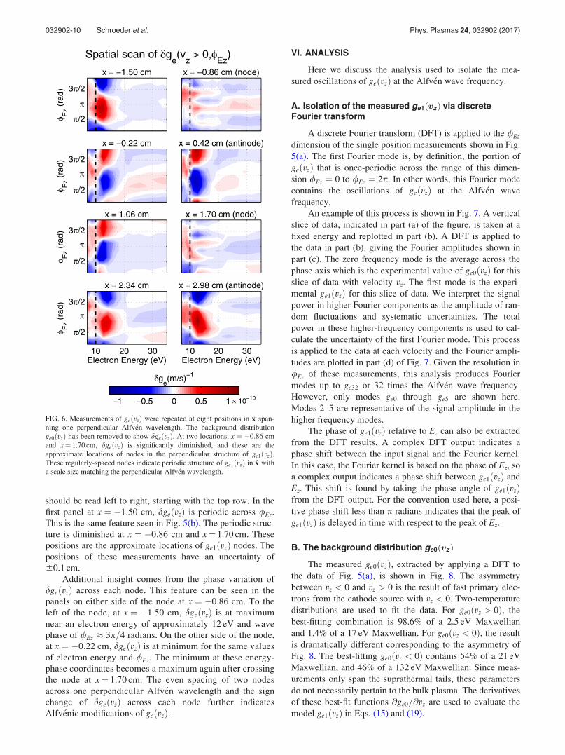
should be read left to right, starting with the top row. In the

first panel at x ¼ �1:50 cm, dgeðvzÞ is periodic across /Ez.

This is the same feature seen in Fig. 5(b). The periodic struc-

ture is diminished at x ¼ �0:86 cm and x¼ 1.70 cm. These

positions are the approximate locations of ge1ðvzÞ nodes. The

positions of these measurements have an uncertainty of

60.1 cm.

Additional insight comes from the phase variation of

dgeðvzÞ across each node. This feature can be seen in the

panels on either side of the node at x ¼ �0:86 cm. To the

left of the node, at x ¼ �1:50 cm, dgeðvzÞ is at maximum

near an electron energy of approximately 12 eV and wave

phase of /Ez � 3p=4 radians. On the other side of the node,

at x ¼ �0:22 cm, dgeðvzÞ is at minimum for the same values

of electron energy and /Ez. The minimum at these energy-

phase coordinates becomes a maximum again after crossing

the node at x¼ 1.70 cm. The even spacing of two nodes

across one perpendicular Alfv�en wavelength and the sign

change of dgeðvzÞ across each node further indicates

Alfv�enic modifications of geðvzÞ.

VI. ANALYSIS

Here we discuss the analysis used to isolate the mea-

sured oscillations of geðvzÞ at the Alfv�en wave frequency.

A. Isolation of the measured ge1ðvzÞ via discreteFourier transform

A discrete Fourier transform (DFT) is applied to the /Ez

dimension of the single position measurements shown in Fig.

5(a). The first Fourier mode is, by definition, the portion of

geðvzÞ that is once-periodic across the range of this dimen-

sion /Ez ¼ 0 to /Ez ¼ 2p. In other words, this Fourier mode

contains the oscillations of geðvzÞ at the Alfv�en wave

frequency.

An example of this process is shown in Fig. 7. A vertical

slice of data, indicated in part (a) of the figure, is taken at a

fixed energy and replotted in part (b). A DFT is applied to

the data in part (b), giving the Fourier amplitudes shown in

part (c). The zero frequency mode is the average across the

phase axis which is the experimental value of ge0ðvzÞ for this

slice of data with velocity vz. The first mode is the experi-

mental ge1ðvzÞ for this slice of data. We interpret the signal

power in higher Fourier components as the amplitude of ran-

dom fluctuations and systematic uncertainties. The total

power in these higher-frequency components is used to cal-

culate the uncertainty of the first Fourier mode. This process

is applied to the data at each velocity and the Fourier ampli-

tudes are plotted in part (d) of Fig. 7. Given the resolution in

/Ez of these measurements, this analysis produces Fourier

modes up to ge32 or 32 times the Alfv�en wave frequency.

However, only modes ge0 through ge5 are shown here.

Modes 2–5 are representative of the signal amplitude in the

higher frequency modes.

The phase of ge1ðvzÞ relative to Ez can also be extracted

from the DFT results. A complex DFT output indicates a

phase shift between the input signal and the Fourier kernel.

In this case, the Fourier kernel is based on the phase of Ez, so

a complex output indicates a phase shift between ge1ðvzÞ and

Ez. This shift is found by taking the phase angle of ge1ðvzÞfrom the DFT output. For the convention used here, a posi-

tive phase shift less than p radians indicates that the peak of

ge1ðvzÞ is delayed in time with respect to the peak of Ez.

B. The background distribution ge0ðvzÞ

The measured ge0ðvzÞ, extracted by applying a DFT to

the data of Fig. 5(a), is shown in Fig. 8. The asymmetry

between vz < 0 and vz > 0 is the result of fast primary elec-

trons from the cathode source with vz < 0. Two-temperature

distributions are used to fit the data. For ge0ðvz > 0Þ, the

best-fitting combination is 98.6% of a 2.5 eV Maxwellian

and 1.4% of a 17 eV Maxwellian. For ge0ðvz < 0Þ, the result

is dramatically different corresponding to the asymmetry of

Fig. 8. The best-fitting ge0ðvz < 0Þ contains 54% of a 21 eV

Maxwellian, and 46% of a 132 eV Maxwellian. Since meas-

urements only span the suprathermal tails, these parameters

do not necessarily pertain to the bulk plasma. The derivatives

of these best-fit functions @ge0=@vz are used to evaluate the

model ge1ðvzÞ in Eqs. (15) and (19).

FIG. 6. Measurements of geðvzÞ were repeated at eight positions in x span-

ning one perpendicular Alfv�en wavelength. The background distribution

ge0ðvzÞ has been removed to show dgeðvzÞ. At two locations, x ¼ �0:86 cm

and x¼ 1.70 cm, dgeðvzÞ is significantly diminished, and these are the

approximate locations of nodes in the perpendicular structure of ge1ðvzÞ.These regularly-spaced nodes indicate periodic structure of ge1ðvzÞ in x with

a scale size matching the perpendicular Alfv�en wavelength.

032902-10 Schroeder et al. Phys. Plasmas 24, 032902 (2017)

C. Amplitude and phase of ge1ðvzÞ

Using a DFT over /Ez to isolate the measured ge1ðvzÞ,we are able to compare theoretical and experimental results.

For this comparison, we only use single-location measure-

ments of Fig. 5 to examine the amplitude and relative phase

of oscillations. Evaluating the model ge1ðvzÞ formed by the

sum of Eqs. (15) and (19) requires several quantities. The

values for Ez, k?, kz, and x are all based on Els€asser probe

measurements of the Alfv�en wave. The derivative @ge0=@vz

comes from the smooth functions fitted to the measured

ge0ðvzÞ seen in Fig. 8. For vz > 0, the boundary z0 is the loca-

tion of the ASW antenna. For vz < 0 z0, is the location of the

cathode. The two free parameters Vs0 and /s of the homoge-

neous solution (Eq. (19)) are determined using least squares

minimization. For vz > 0; Vs0 ¼ 0:84 V and /s ¼ 0:27 radi-

ans. For vz < 0, Vs0 ¼ 0:97 V and /s ¼ 2:53 radians. A non-

zero value of Vs0 for vz < 0 indicates the cathode-anode volt-

age is modulated at the frequency of the Alfv�en wave, a pro-

cess that is not well understood. The free parameters Vs0 and

/s are scalar values that do not depend on vz. The form of

the homogeneous solution as a function of vz is not adjusted

in the least squares determination of these quantities.

Fig. 9 shows the direct, quantitative comparison of the

measured and modeled ge1ðvzÞ. The amplitude of each data

point in part (a) of this figure shows how intensely that por-

tion of the reduced parallel electron distribution function

oscillates during the inertial Alfv�en wave pulse. The phase

of the data points in part (b) shows whether the oscillations

ge1ðvzÞ lead or lag Ez of the Alfv�en wave. For the phase con-

vention used here, a positive phase shift less than p radians

relative to /Ez indicates the oscillations of geðvzÞ lag Ez. The

measured ge1ðvzÞ lags Ez. Overall, the model agrees with

measurements within the error bars. This is believed to be

the first demonstration of quantitative agreement between

measured oscillations of the suprathermal parallel electron

distribution and linear kinetic theory of an inertial Alfv�en

wave. While the uniqueness of our model cannot be abso-

lutely guaranteed without repeating this experiment at sev-

eral locations in the parallel z direction, the quantitative

agreement of the model with measurements is promising.

D. Spatial structure of ge1ðvz Þ

Using measurements from multiple locations, it is possi-

ble to examine the spatial structure of the measured ge1ðvzÞand compare with predictions. The idealized Ez waveform in

Eq. (5) and the full solution for ge1ðvzÞ in Eqs. (15) and (19)

FIG. 7. A DFT is applied over /Ez to

isolate oscillations of geðvzÞ at the

Alfv�en wave frequency. (a) To demon-

strate this technique, measurements at

a fixed energy E¼ 29 eV are taken

from the full data set. (b) The slice of

data at fixed energy is replotted. The

fundamental mode over /Ez seen here

is the measured ge1ðvzÞ at this energy.

(c) The measured ge1ðvzÞ is isolated

using a DFT over /Ez. The zero fre-

quency mode (average) is the mea-

sured ge0ðvzÞ, and the first order mode

is ge1ðvzÞ. Power in higher frequencies

is the result of random and systematic

errors. (d) This technique is extended

to data at each energy to isolate ge0ðvzÞand ge1ðvzÞ. Higher frequency modes

generally have lower amplitude than

ge1ðvzÞ and are interpreted as the

amplitude of random fluctuations and

systematic uncertainties.

FIG. 8. The background distribution function ge0ðvzÞ is extracted from the

full set of geðvzÞ measurements in Fig. 5(a). Smooth functions are fitted to

the measurements, and the derivaties of these functions are used to evaluate

the model ge1ðvzÞ. The asymmetry seen here is a result of primary electrons

from the cathode with vz < 0. The uncertainty of measurements is shown in

gray.

032902-11 Schroeder et al. Phys. Plasmas 24, 032902 (2017)

vary like cosðk?xÞ, so that the variations in these quantities

are predicted to be aligned in x. The DFT analysis described

in Section VI A is applied to the data from all eight locations

in Fig. 6. The intensity of ge1ðvzÞ from each location is

mapped in Fig. 10. This figure shows the measured values of

By and the calculated values of Ez along the range of the scan

taken from Fig. 2. Notably, the measured ge1ðvzÞ is most

intense at the antinodes of Ez and is diminished at the nodes

of Ez. This confirms the prediction that variations of ge1ðvzÞand Ez are aligned in x.

E. Relative importance of the homogeneous solution

The model ge1ðvzÞ includes the terms ge1fðvzÞ þ ge1kðvzÞthat are attributable to the Alfv�en wave and an additional

homogeneous solution ge1hðvzÞ used to describe non-

Alfv�enic perturbations at the same frequency as the Alfv�en

wave. It is worth considering the relative importance of the

Alfv�enic and non-Alfv�enic terms. While the experimental

data cannot answer this question, the model can provide

insight.

Fig. 11 shows the amplitude of the Alfv�en wave terms

and the homogeneous solution. Consider the two halves of

this plot separately. For vz > 0, where the boundary is the

ASW antenna, the Alfv�enic and non-Alfv�enic contributions

are approximately equal in amplitude. Since the ASW

antenna functions by applying an oscillating voltage to the

plasma, the importance of the homogeneous solution which

includes an oscillating voltage boundary condition is

expected. For vz < 0, the boundary is the cathode. The sig-

nificance of the homogeneous solution for this half of the

data implies the cathode-anode voltage is oscillating at the

frequency of the Alfv�en wave. The presence of an oscillating

voltage at this boundary is not well understood. An expected

feature, confirmed by Fig. 11, is that the Alfv�en wave terms

FIG. 11. The amplitudes of the Alfv�en wave solution and the homogeneous

solution are shown here. According to the model, both the homogeneous

solution and the Alfv�en wave solution are significant for vz > 0. For vz < 0,

the homogeneous solution dwarfs the Alfv�en wave terms. The insignificance

of the Alfv�en wave solution for vz < 0 is expected since this is the non-

resonant direction.

FIG. 9. The linear model accurately describes the amplitude and phase of

ge1ðvzÞ measurements taken at a single location. (a) An absolute comparison

of the amplitude of the measured and modeled ge1ðvzÞ shows good agree-

ment. The model curve is produced by evaluating Eqs. (15) and (19). (b)

Plotted here is the phase of ge1ðvzÞ relative to the phase of Ez. The model is

able to replicate the relative phase of the measured ge1ðvzÞ. Above E ¼ þ50

eV, experimental uncertainty approaches 2p, so that phase data in this range

is not meaningful. The uncertainty of measurements is shown in gray.

FIG. 10. The measurement process is repeated in an abbreviated form at

8 locations in x spanning one perpendicular Alfv�en wavelength. The top

panel shows the measured By and the calculated Ez for the same range in x.

Measurements of By are used to calculate Ez. Errors in By measurements are

smaller than the markers. The bottom panel is an intensity map showing var-

iations in the strength of measured ge1ðvzÞ along the scan. The significant

result seen here is that the measured ge1ðvzÞ vanishes at the nodes of Ez, as

predicted.

032902-12 Schroeder et al. Phys. Plasmas 24, 032902 (2017)

are more significant for vz > 0 than for vz < 0. This is

expected since vz > 0 is the resonant direction and the

denominator of the Alfv�enic terms in Eq. (15) goes to zero

as the velocity approaches resonance.

A new antenna has been built that inductively couples to

the Alfv�en wave instead of electrostatically like the ASW

antenna. The electrostatic design of the ASW antenna may

be responsible for the prominence of the homogeneous term.

The new inductively-coupled antenna is designed to reduce

the homogeneous term.

F. Validity of the model boundary term assumptions

The experimental measurement of ge1ðvzÞ enables addi-

tional analysis of assumptions used to produce the homoge-

neous solution in Eq. (19). The full solution is the sum ge1

¼ ge1f þ ge1k þ ge1h. Rearranging gives ge1h ¼ ge1 � ge1f

�ge1k. Using this rearranged form along with data for ge1ðvzÞand theoretical values for ge1fðvzÞ and ge1kðvzÞ gives values

for ge1hðvzÞ as a hybrid of data and theory. The benefit of this

hybrid is that ge1hðvzÞ is evaluated using a different set of

assumptions from the ones used in Section IV D to produce

the analytical expression for ge1hðvzÞ. The hybrid values

require both the assumptions of the measurement and analysis

techniques to produce the measured ge1ðvzÞ and the assump-

tions used to produce the analytical form of the Alfv�en wave

terms ge1f ðvzÞ þ ge1kðvzÞ (Eq. (15)). Conversely, the analytical

form of ge1ðvzÞ assumed there is an oscillating voltage at the

boundary producing a non-Alfv�enic perturbation in the motion

of the suprathermal electrons. Fig. 12 compares the hybrid

values for ge1hðvzÞ with values of the analytical expression for

ge1hðvzÞ (Eq. (19)). There is good agreement, indicating the

non-Alfv�enic effects of the ASW antenna are sufficiently

described by the homogeneous solution developed in Section

IV D and justifying the use of this homogeneous solution in

the analysis.

VII. CONCLUSION

This research investigated the oscillations of the reduced

parallel electron distribution function ge1ðvzÞ caused by an

inertial Alfv�en wave. Unlike the Alfv�en waves of ideal

MHD, inertial Alfv�en waves have a parallel electric field

that causes oscillations in the parallel electron motion and is

expected to produce accelerated electrons. Until this study,

neither effect had been definitively verified. The acceleration

of electrons by inertial Alfv�en waves likely contributes to

the generation of a significant fraction of auroras, and the

suprathermal portion of geðvzÞ is of particular interest since

the acceleration affects electrons above the thermal speed.

Measurements were carried out in UCLA’s Large Plasma

Device (LAPD) using the Whistler Wave Absorption

Diagnostic (WWAD), an electron cyclotron absorption diag-

nostic that accurately measures the suprathermal tails of

geðvzÞ. Using a series of phase-shifted data sets, we produced

a composite measurement of geðvzÞ with sufficient resolution

in Alfv�en wave phase to isolate oscillations at the Alfv�en

wave frequency. The model for these oscillations ge1ðvzÞ,derived from the linearized gyroaveraged Boltzmann equa-

tion, includes an Alfv�en wave solution and an additional

homogeneous solution that accounts for non-Alfv�enic effects

generated by the antenna. The model accurately reproduces

the amplitude, phase, and spatial structure of the measured

oscillations. By measuring and modeling the linear oscilla-

tions of geðvzÞ, this experiment verifies one of the funda-

mental distinctions between ideal MHD and inertial Alfv�en

waves. While plasma in the lower magnetosphere is colli-

sionless, in this experiment the inertial Alfv�en wave and

the electron response ge1ðvzÞ are modified by electron colli-

sions. However, since the suprathermal electrons are signif-

icantly less collisional than the thermal electrons, the

properties of the suprathermal portions of the measured and

modeled ge1ðvzÞ are not fundamentally distinct from the col-

lisionless scenario.

Having successfully measured and modeled the linear

oscillations of the reduced electron distribution function, we

turn our attention to the nonlinear Alfv�en wave-particle

physics. Ongoing experiments are testing a new higher-

power Alfv�en wave antenna and exploring the use of innova-

tive analysis techniques that employ field-particle correla-

tions to directly compute the rate of energy transfer between

the parallel electric field and the electrons.27

FIG. 12. The model for the homogeneous solution ge1hðvzÞ produced in

Section IV D uses a number of assumptions, and the effectiveness of these

assumptions is tested by comparing the model and hybrid values of ge1hðvzÞ.Part (a) shows the amplitude and part (b) shows the phase of ge1hðvsÞ. There

is good agreement between the model and the hybrid, indicating that the

assumptions used in the derivation of ge1hðvzÞ are sufficient to describe the

non-Alfv�enic perturbations originating at the boundary. The uncertainty of

the hybrid values is shown in gray.

032902-13 Schroeder et al. Phys. Plasmas 24, 032902 (2017)

ACKNOWLEDGMENTS

This work was supported by the NSF Graduate Research

Fellowship under Grant No. 1048957, NSF Grant Nos. ATM

03-17310 and PHY-10033446, NSF CAREER Award No.

AGS-1054061, DOE Grant No. DE-SC0014599, and NASA

Grant No. NNX10AC91G. The experiment presented here

was conducted at the Basic Plasma Science Facility, funded

by the U.S. Department of Energy and the National Science

Foundation. The data used are available from the

corresponding author upon request.

This work is part of a dissertation to be submitted by J.

W. R. Schroeder to the Graduate College, University of Iowa,

Iowa City, IA, in partial fulfillment of the requirements for the

Ph.D. degree in Physics.

1A. Keiling, “Alfv�en waves and their roles in the dynamics of the Earth’s

magnetotail: A review,” Space Sci. Rev. 142, 73–156 (2009).2K. Stasiewicz, P. Bellan, C. Chaston, C. Kletzing, R. Lysak, J. Maggs, O.

Pokhotelov, C. Seyler, P. Shukla, L. Stenflo, A. Streltsov, and J.-E.

Wahlund, “Small scale alfv�enic structure in the aurora,” Space Sci. Rev.

92, 423–533 (2000).3A. Hasegawa, “Particle acceleration by MHD surface wave and formation

of aurora,” J. Geophys. Res. 81, 5083–5090, doi:10.1029/JA081i028p05083

(1976).4C. C. Chaston, C. W. Carlson, J. P. McFadden, R. E. Ergun, and R. J.

Strangeway, “How important are dispersive Alfv�en waves for auroral par-

ticle acceleration?,” Geophys. Res. Lett. 34, L07101, doi:10.1029/

2006GL029144 (2007).5C. K. Goertz and R. W. Boswell, “Magnetosphere-ionosphere coupling,”

J. Geophys. Res. 84, 7239–7246, doi:10.1029/JA084iA12p07239 (1979).6C. A. Kletzing and S. Hu, “Alfv�en wave generated electron time dispersion,”

Geophys. Res. Lett. 28, 693–696, doi:10.1029/2000GL012179 (2001).7A. Keiling, J. R. Wygant, C. Cattell, W. Peria, G. Parks, M. Temerin, F. S.

Mozer, C. T. Russell, and C. A. Kletzing, “Correlation of Alfv�en wave

poynting flux in the plasma sheet at 4-7 RE with ionospheric electron energy

flux,” J. Geophys. Res. 107, 1132, doi:10.1029/2001JA900140 (2002).8C. C. Chaston, J. W. Bonnell, C. W. Carlson, J. P. McFadden, R. E. Ergun,

and R. J. Strangeway, “Properties of small-scale Alfv�en waves and accel-

erated electrons from FAST,” J. Geophys. Res. 108, 8003, doi:10.1029/

2002JA009420 (2003).9C. C. Chaston, “ULF waves and auroral electrons,” in MagnetosphericULF Waves: Synthesis and New Directions, American Geophysical Union

Geophysical Monograph Series, edited by K. Takahashi, P. J. Chi, R. E.

Denton, and R. L. Lysak (American Geophysical Union, Washington, DC,

2006), Vol. 169, p. 239.10D. Schriver, M. Ashour-Abdalla, R. J. Strangeway, R. L. Richard, C.

Klezting, Y. Dotan, and J. Wygant, “FAST/Polar conjunction study of

field-aligned auroral acceleration and corresponding magnetotail drivers,”

J. Geophys. Res. 108, 8020, doi:10.1029/2002JA009426 (2003).11W. Gekelman, P. Pribyl, Z. Lucky, M. Drandell, D. Leneman, J. Maggs, S.

Vincena, B. Van Compernolle, S. K. P. Tripathi, G. Morales, T. A. Carter,

Y. Wang, and T. DeHaas, “The upgraded large plasma device, a machine

for studying frontier basic plasma physics,” Rev. Sci. Instrum. 87, 025105

(2016).12D. J. Thuecks, F. Skiff, and C. A. Kletzing, “Measurements of parallel

electron velocity distributions using whistler wave absorption,” Rev. Sci.

Instrum. 83, 083503 (2012).13J. W. R. Schroeder, F. Skiff, C. A. Kletzing, G. G. Howes, T. A. Carter,

and S. Dorfman, “Direct measurement of electron sloshing of an inertial

Alfv�en wave,” Geophys. Res. Lett. 43, 4701–4707, doi:10.1002/

2016GL068865 (2016).14R. L. Lysak and W. Lotko, “On the kinetic dispersion relation for shear

Alfv�en waves,” J. Geophys. Res. 101, 5085–5094, doi:10.1029/

95JA03712 (1996).15J. D. Huba, Plasma Physics (Naval Research Laboratory, Washington,

DC, 2013), pp. 1–71.16D. J. Thuecks, C. A. Kletzing, F. Skiff, S. R. Bounds, and S. Vincena,

“Tests of collision operators using laboratory measurements of shear

Alfv�en wave dispersion and damping,” Phys. Plasmas 16, 052110

(2009).17C. A. Kletzing, D. J. Thuecks, F. Skiff, S. R. Bounds, and S. Vincena,

“Measurements of inertial limit Alfv�en wave dispersion for finite perpen-

dicular wave number,” Phys. Rev. Lett. 104, 095001 (2010).18C. A. Kletzing, “Electron acceleration by kinetic Alfv�en waves,”

J. Geophys. Res. 99, 11095–11104, doi:10.1029/94JA00345 (1994).19D. J. Drake, C. A. Kletzing, F. Skiff, G. G. Howes, and S. Vincena,

“Design and use of an Els€asser probe for analysis of Alfv�en wave fields

according to wave direction,” Rev. Sci. Instrum. 82, 103505 (2011).20R. M. Kulsrud, “MHD description of plasma,” in Basic Plasma Physics I,

Handbook of Plasma Physics, edited by A. A. Galeev and R. N. Sudan

(North Holland, 1983), Vol. 1, Chap. 1.4, pp. 115–145.21T. G. Northrop, “The guiding center approximation to charged particle

motion,” Ann. Phys. 15, 79–101 (1961).22D. A. Gurnett and A. Bhattacharjee, in Introduction to Plasma Physics

(Cambridge University Press, Cambridge, UK, 2005).23R. Kirkwood, I. Hutchinson, S. Luckhardt, and J. Squire, “Measurement of

suprathermal electrons in tokamaks via electron cyclotron transmission,”

Nucl. Fusion 30, 431 (1990).24F. Skiff, D. A. Boyd, and J. A. Colborn, “Measurements of electron

parallel-momentum distributions using cyclotron wave transmission*,”

Phys. Fluids B 5, 2445–2450 (1993).25F. Skiff, D. A. Boyd, and J. A. Colborn, “Measurements of electron

dynamics during lower hybrid current drive,” Plasma Phys. Controlled

Fusion 36, 1371–1379 (1994).26T. H. Stix, Waves in Plasmas (American Institute of Physics, New York,

1992).27K. G. Klein and G. G. Howes, “Measuring collisionless damping in helio-

spheric plasmas using field-particle correlations,” Astrophys. J. Lett. 826,

L30 (2016).

032902-14 Schroeder et al. Phys. Plasmas 24, 032902 (2017)