linear systems - dynamical systemsmurray/books/am05/pdf/am06-linsys_16sep06.… · linear systems...

Chapter 5

Linear Systems

Few physical elements display truly linear characteristics. For example therelation between force on a spring and displacement of the spring is alwaysnonlinear to some degree. The relation between current through a resistor andvoltage drop across it also deviates from a straight-line relation. However, ifin each case the relation is ?reasonably? linear, then it will be found that thesystem behavior will be very close to that obtained by assuming an ideal, linearphysical element, and the analytical simplification is so enormous that wemake linear assumptions wherever we can possibly to so in good conscience.

R. Cannon, Dynamics of Physical Systems, 1967 [Can03].

In Chapters 2–4 we considered the construction and analysis of differen-tial equation models for physical systems. We placed very few restrictionson these systems other than basic requirements of smoothness and well-posedness. In this chapter we specialize our results to the case of linear,time-invariant, input/output systems. This important class of systems isone for which a wealth of analysis and synthesis tools are available, andhence it has found great utility in a wide variety of applications.

5.1 Basic Definitions

We have seen several examples of linear differential equations in the ex-amples of the previous chapters. These include the spring mass system(damped oscillator) and the operational amplifier in the presence of small(non-saturating) input signals. More generally, many physical systems canbe modeled very accurately by linear differential equations. Electrical cir-cuits are one example of a broad class of systems for which linear models canbe used effectively. Linear models are also broadly applicable in mechani-

143

144 CHAPTER 5. LINEAR SYSTEMS

cal engineering, for example as models of small deviations from equilibria insolid and fluid mechanics. Signal processing systems, including digital filtersof the sort used in CD and MP3 players, are another source of good exam-ples, although often these are best modeled in discrete time (as described inmore detail in the exercises).

In many cases, we create systems with linear input/output responsethrough the use of feedback. Indeed, it was the desire for linear behav-ior that led Harold S. Black, who invited the negative feedback amplifier,to the principle of feedback as a mechanism for generating amplification.Almost all modern single processing systems, whether analog or digital, usefeedback to produce linear or near-linear input/output characteristics. Forthese systems, it is often useful to represent the input/output characteristicsas linear, ignoring the internal details required to get that linear response.

For other systems, nonlinearities cannot be ignored if one cares aboutthe global behavior of the system. The predator prey problem is one exam-ple of this; to capture the oscillatory behavior of the coupled populationswe must include the nonlinear coupling terms. However, if we care aboutwhat happens near an equilibrium point, it often suffices to approximatethe nonlinear dynamics by their local linearization, as we already exploredbriefly in Section 4.3. The linearization is essentially an approximation ofthe nonlinear dynamics around the desired operating point.

Linearity

We now proceed to define linearity of input/output systems more formally.Consider a state space system of the form

dx

dt= f(x, u)

y = h(x, u),(5.1)

where x ∈ Rn, u ∈ R

p and y ∈ Rq. As in the previous chapters, we will

usually restrict ourselves to the single input, single output case by takingp = q = 1. We also assume that all functions are smooth and that for areasonable class of inputs (e.g., piecewise continuous functions of time) thatthe solutions of equation (5.1) exist for all time.

It will be convenient to assume that the origin x = 0, u = 0 is anequilibrium point for this system (x = 0) and that h(0, 0) = 0. Indeed, wecan do so without loss of generality. To see this, suppose that (xe, ue) 6= (0, 0)is an equilibrium point of the system with output ye = h(xe, ue) 6= 0. Then

5.1. BASIC DEFINITIONS 145

we can define a new set of states, inputs, and outputs

x = x− xe u = u− ue y = y − ye

and rewrite the equations of motion in terms of these variables:

d

dtx = f(x+ xe, u+ ue) =: f(x, u)

y = h(x+ xe, u+ ue) − ye =: h(x, u).

In the new set of variables, we have that the origin is an equilibrium pointwith output 0, and hence we can carry our analysis out in this set of vari-ables. Once we have obtained our answers in this new set of variables, wesimply have to remember to “translate” them back to the original coordi-nates (through a simple set of additions).

Returning to the original equations (5.1), now assuming without loss ofgenerality that the origin is the equilibrium point of interest, we write theoutput y(t) corresponding to initial condition x(0) = x0 and input u(t) asy(t;x0, u). Using this notation, a system is said to be a linear input/outputsystem if the following conditions are satisfied:

(i) y(t;αx1 + βx2, 0) = αy(t;x1, 0) + βy(t;x2, 0)

(ii) y(t;αx0, δu) = αy(t;x0, 0) + δy(t; 0, u)

(iii) y(t; 0, δu1 + γu2) = δy(t; 0, u1) + γy(t; 0, u2).

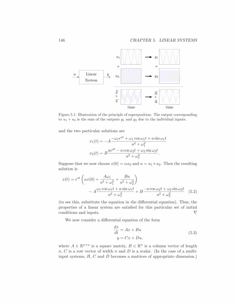
Thus, we define a system to be linear if the outputs are jointly linear in theinitial condition response and the forced response. Property (ii) is the usualdecomposition of a system response into the homogeneous response (u = 0)and the particular response (x0 = 0). Property (iii) is the formal definitionof the the principle of superposition illustrated in Figure 5.1.

Example 5.1 (Scalar system). Consider the first order differential equation

dx

dt= ax+ u

y = x

with x(0) = x0. Let u1 = A sinω1t and u2 = B cosω2t. The homogeneoussolution the ODE is

xh(t) = eatx0


time

u yLinear

Systemy2

u1

+

u2

u1

+u

2

y 1+y 2

+

y1

time

Figure 5.1: Illustration of the principle of superposition. The output correspondingto u1 + u2 is the sum of the outputs y1 and y2 due to the individual inputs.

and the two particular solutions are

x1(t) = −A−ω1eat + ω1 cosω1t+ a sinω1t

a2 + ω21

x2(t) = Baeat − a cosω2t+ ω2 sinω2t

a2 + ω22

.

Suppose that we now choose x(0) = αx0 and u = u1+u2. Then the resultingsolution is

x(t) = eat

(

αx(0) +Aω1

a2 + ω21

+Ba

a2 + ω22

)

−Aω1 cosω1t+ a sinω1t

a2 + ω21

+B−a cosω2t+ ω2 sinω2t

a2 + ω22

(5.2)

(to see this, substitute the equation in the differential equation). Thus, theproperties of a linear system are satisfied for this particular set of initialconditions and inputs. ∇

We now consider a differential equation of the form

dx

dt= Ax+Bu

y = Cx+Du,(5.3)

where A ∈ Rn×n is a square matrix, B ∈ R

n is a column vector of lengthn, C is a row vector of width n and D is a scalar. (In the case of a multi-input systems, B, C and D becomes a matrices of appropriate dimension.)

5.1. BASIC DEFINITIONS 147

Equation (5.3) is a system of linear, first order, differential equations withinput u, state x and output y. We now show that this system is a linearinput/output system, in the sense described above.

Proposition 5.1. The differential equation (5.3) is a linear input/outputsystem.

Proof. Let xh1(t) and xh2(t) be the solutions of the linear differential equa-tion (5.3) with input u(t) = 0 and initial conditions x(0) = x01 and x02,respectively, and let xp1(t) and xp2(t) be the solutions with initial conditionx(0) = 0 and inputs u1(t), u2(t) ∈ R. It can be verified by substitution thatthe solution of equation (5.3) with initial condition x(0) = αx01 + βx02 andinput u(t) = δu1 + γu2 and is given by

x(t) =(αxh1(t) + βxh2(t)

)+(δxp1(t) + γxp2(t)

).

The corresponding output is given by

y(t) =(αyh1(t) + βyh2(t)

)+(δyp1(t) + γyp2(t)

).

By appropriate choices of α, β, δ and γ, properties (i)–(iii) can be verified.

As in the case of linear differential equations in a single variable, wedefine the solution xh(t) with zero input as the homogeneous solution andthe solution xp(t) with zero initial condition as the particular solution. Fig-ure 5.2 illustrates how these the homogeneous and particular solutions canbe superposed to form the complete solution.

It is also possible to show that if a system is input/output linear in thesense we have described, that it can always be represented by a state spaceequation of the form (5.3) through appropriate choice of state variables.

Time Invariance

Time invariance is another important concept that is can be used to describea system whose properties do not change with time. More precisely, ifthe input u(t) gives output y(t), then if we shift the time at which theinput is applied by a constant amount a, u(t + a) gives the output y(t +a). Systems that are linear and time-invariant, often called LTI systems,have the interesting property that their response to an arbitrary input iscompletely characterized by their response to step inputs or their responseto short “impulses”.


0 20 40 60−2

−1

0

1

2

Hom

ogen

eous

Input (u)

0 20 40 60−2

−1

0

1

2

State (x1, x

2)

0 20 40 60−2

−1

0

1

2Output (y)

0 20 40 60−2

−1

0

1

2

Par

ticul

ar

0 20 40 60−2

−1

0

1

2

0 20 40 60−2

−1

0

1

2

0 20 40 60−2

−1

0

1

2

Com

plet

e

time (sec)0 20 40 60

−2

−1

0

1

2

time (sec)0 20 40 60

−2

−1

0

1

2

time (sec)

Figure 5.2: Superposition of homogeeous and particular solutions. The first rowshows the input, state and output corresponding to the initial condition response.The second row shows the same variables corresponding to zero initial condition,but nonzero input. The third row is the complete solution, which is the sume ofthe two individual solutions.

We will first compute the response to a piecewise constant input. Assumethat the sytem is initially at rest and consider the piecewise constant inputshown in Figure 5.3a. The input has jumps at times tk and its values afterthe jumps are u(tk). The input can be viewed as a combination of steps:the first step at time t0 has amplitude u(t0), the second step at time t1 hasamplitude u(t1) − u(t0), etc.

Assuming that the system is initially at an equilibrium point (so thatthe initial condition response is zero), the response to the input can then beobtained by superimposing the responses to a combination of step inputs.Let H(t) be the response to a unit step applied at time t. The responseto the first step is then H(t − t0)u(t0), the response to the second step is

5.2. THE CONVOLUTION EQUATION 149

0 2 4 6 8 100

0.2

0.4

0.6

0.8

1

Time (sec)

Inpu

t (u)

u(t0)

u(t1) u(t

1) − u(t

0)

(a)

0 2 4 6 8 10−0.2

0

0.2

0.4

0.6

0.8

1

1.2

Time (sec)

Out

put (

y)

(b)

Figure 5.3: Response to piecewise constant inputs: (a) a piecewise constant signalcan be represented as a sum of step signals; (b) the resulting output is the sum ofthe individual outputs.

H(t− t1)(u(t1)−u(t0)

), and we find that the complete response is given by

y(t) = H(t− t0)u(t0) +H(t− t1)(u(t1) − u(t0)

)+ · · ·

=(H(t) −H(t− t1)

)u(t0) +

(H(t− t1) −H(t− t2)

)u(t1)

=∞∑

n=0

(H(t− tn) −H(t− tn+1)

)u(tn)

=∞∑

n=0

H(t− tn) −H(t− tn+1)

tn+1 − tn

(tn+1 − tn

)u(tn).

An example of this computation is shown in Figure 5.3b.The response to a continuous input signal is obtained by taking the limit

as tn+1 − tn → 0, which gives

y(t) =

∫∞

0H ′(t− τ)u(τ)dτ, (5.4)

where H ′ is the derivative of the step response, which is also called the im-pulse response. The response of a linear time-invariant system to any inputcan thus be computed from the step response. We will derive equation (5.4)in a slightly different way in the next section.

5.2 The Convolution Equation

Equation (5.4) shows that the input response of a linear system can bewritten as an integral over the inputs u(t). In this section we derive a more


general version of this formula, which shows how to compute the output ofa linear system based on its state space representation.

The Matrix Exponential

Although we have shown that the solution of a linear set of differential equa-tions defines a linear input/output system, we have not fully computed thesolution of the system. We begin by considering the homogeneous responsecorresponding to the system

dx

dt= Ax. (5.5)

For the scalar differential equation

x = ax x ∈ R, a ∈ R

the solution is given by the exponential

x(t) = eatx(0).

We wish to generalize this to the vector case, where A becomes a matrix.

We define the matrix exponential as the infinite series

eX = I +X +1

2X2 +

1

3!X3 + · · · =

∞∑

k=0

1

k!Xk, (5.6)

where X ∈ Rn×n is a square matrix and I is the n× n identity matrix. We

make use of the notation

X0 = I X2 = XX Xn = Xn−1X,

which defines what we mean by the “power” of a matrix. Equation (5.6) iseasy to remember since it is just the Taylor series for the scalar exponential,applied to the matrix X. It can be shown that the series in equation (5.6)converges for any matrix X ∈ R

n×n in the same way that the normal expo-nential is defined for any scalar a ∈ R.

Replacing X in equation (5.6) by At where t ∈ R we find that

eAt = I +At+1

2A2t2 +

1

3!A3t3 + · · · =

∞∑

k=0

1

k!Aktk,


and differentiating this expression with respect to t gives

d

dteAt = A+At+

1

2A3t2 + · · · = A

∞∑

k=0

1

k!Aktk = AeAt. (5.7)

Multiplying by x(0) from the right we find that x(t) = eAtx(0) is the solutionto the differential equation (5.5) with initial condition x(0). We summarizethis important result as a theorem.

Theorem 5.2. The solution to the homogeneous system of differential equa-tion (5.5) is given by

x(t) = eAtx(0).

Notice that the form of the solution is exactly the same as for scalarequations.

The form of the solution immediately allows us to see that the solutionis linear in the initial condition. In particular, if xh1 is the solution toequation (5.5) with initial condition x(0) = x01 and xh2 with initial conditionx02, then the solution with initial condition x(0) = αx01 + βx02 is given by

x(t) = eAt(αx01 + βx02

)=(αeAtx01 + βeAtx02) = αxh1(t) + βxh2(t).

Similarly, we see that the corresponding output is given by

y(t) = Cx(t) = αyh1(t) + βyh2(t),

where yh1 and yh2 are the outputs corresponding to xh1 and xh2.

We illustrate computation of the matrix exponential by three examples.

Example 5.2 (Double integrator). A very simple linear system that is usefulfor understanding basic concepts is the second order system given by

q = u

y = q.

This system system is called a double integrator because the input u isintegrated twice to determine the output y.

In state space form, we write x = (q, q) and

dx

dt=

0 10 0

x+

01

u.


The dynamics matrix of a double integrator is

A =

0 10 0

and we find by direct calculation that A2 = 0 and hence

eAt =

1 t0 1

.

Thus the homogeneous solution (u = 0) for the double integrator is givenby

x(t) =

x1(0) + tx2(0)

x2(0)

y(t) = x1(0) + tx2(0).

∇

Example 5.3 (Undamped oscillator). A simple model for an oscillator, suchas the spring mass system with zero damping, is

mq + kq = u.

Putting the system into state space form, the dynamics matrix for thissystem is

A =

0 1

− km 0

We have

eAt =

cosω0t

1ω0

sinω0t

−ω0 sinω0t cosω0t

ω0 =

√

k

m,

and the solution is then given by

x(t) = eAtx(0) =

cosω0t

1ω0

sinω0t


x1(0)x2(0)

.

This solution can be verified by differentiation:

d

dtx(t) =

−ω0 sinω0t cosω0t−ω2

0 cosω0t −ω0 sinω0t

x1(0)x2(0)

.

=

0 1

−ω20 0

cosω0t

1ω0

sinω0t


x1(0)x2(0)

= Ax(t).


If the damping c is nonzero, the solution is more complicated, but the matrixexponential can be shown to be

eAt = e−ct

2m

eωdt + e−ωdt

2+eωdt − e−ωdt

2√c2 − 4km

eωdt − e−ωdt

√c2 − 4km

−keωdt − ke−ωdt

√c2 − 4km

eωdt + e−ωdt

2− ceωdt − ce−ωdt

2√c2 − 4km

,

where ωd =√c2 − 4km/2m. Note that ωd can either be real or complex,

but in the case it is complex the combinations of terms will always yield apositive value for the entry in the matrix exponential. ∇

Example 5.4 (Diagonal system). Consider a diagonal matrix

A =

λ1 0λ2

. . .

0 λn

The kth power of At is also diagonal,

(At)k =

λk1t

k 0λk

2tk

. . .

0 λknt

k

and it follows from the series expansion that the matrix exponential is givenby

eAt =

eλ1t 0eλ2t

. . .

0 eλnt

.

∇

Eigenvalues and Modes

The initial condition response of a linear system can be written in terms of amatrix exponential involving the dynamics matrix A. The properties of thematrix A therefore determine the resulting behavior of the system. Given a


matrix A ∈ Rn×n, recall that λ is an eigenvalue of A with eigenvector v if λ

and v satisfyAv = λv.

In general λ and v may be complex valued, although if A is real-valued thenfor any eigenvalue λ, its complex conjugate λ∗ will also be an eigenvalue(with v∗ as the corresponding eigenvector).

Suppose first that λ and v are a real-valued eigenvalue/eigenvector pairfor A. If we look at the solution of the differential equation for x(0) = v, itfollows from the definition of the matrix exponential that

eAtv =(I +At+

1

2A2t2 + · · ·

)v = (v + λtv +

λ2t2

2v + · · ·

)v = eλtv.

The solution thus lies in the subspace spanned by the eigenvector. Theeigenvalue λ describes how the solution varies in time and is often called amode of the system. If we look at the individual elements of the vectors xand v, it follows that

xi(t)

xj(t)=vi

vk,

and hence the ratios of the components of the state x are constants. Theeigenvector thus gives the “shape” of the solution and is also called a modeshape of the system.

Figure 5.4 illustrates the modes for a second order system. Notice thatthe state variables have the same sign for the slow mode λ = −0.08 anddifferent signs for the fast mode λ = −0.62.

The situation is a little more complicated when the eigenvalues of A arecomplex. Since A has real elements, the eigenvalues and the eigenvectorsare complex conjugates

λ = σ ± jω and v = u± jw,

which implies that

u =v + v∗

2w =

v − v∗

2j.

Making use of the matrix exponential, we have

eAtv == eλt(u+ jw) = eσt((u cosωt− w sinωt) + j(u sinωt+ w cosωt)

),

which implies

eAtu =1

2

(

eAtv + eAtv∗)

= ueσt cosωt− weσt sinωt

eAtw =1

2j

(

eAtv − eAtv∗)

= ueσt sinωt+ weσt cosωt.


−1 −0.5 0 0.5 1−1

−0.5

0

0.5

1

x1

x2

(a)

0 10 20 30 40 500

0.5

1

0 10 20 30 40 50

0

0.5

1

x1,x

2x

1,x

2

Slow mode λ = −0.08

Fast mode λ = −0.62

(b)

Figure 5.4: Illustration of the notion of modes for a second order system with realeigenvalues. The left figure (a) shows the phase plane and the modes correspondsto solutions that start on the eigenvectors. The time functions are shown in (b).The ratios of the states are also computed to show that they are constant for themodes.

A solution with initial conditions in the subspace spanned by the real partu and imaginary part v of the eigenvector will thus remain in that subspace.The solution will be logarithmic spiral characterized by σ and ω. We againcall λ a mode of the system and v the mode shape.

If a matrix A has a n distinct eigenvalues λ1, . . . , λn, then the initial con-dition response can be written as a linear combination of the modes. To seethis, suppose for simplicity that we have all real eigenvalues with correspond-ing unit eigenvectors v1, . . . , vn. From linear algebra, these eigenvectors arelinearly independent and we can write the initial condition x(0) as

x(0) = α1v1 + α2v2 + · · ·αnvn.

Using linearity, the initial condition response can be written as

x(t) = α1eλ1tv1 + α2e

λ2tv2 + · · · + αneλntvn.

Thus, the response is a linear combination the modes of the system, withthe amplitude of the individual modes growing or decaying as eλit. The casefor distinct complex eigenvalues follows similarly (the case for non-distincteigenvalues is more subtle and is described in the section on the Jordanform, below).


Linear Input/Output Response

We now return to the general input/output case in equation (5.3), repeatedhere:

dx

dt= Ax+Bu

y = Cx+Du.(5.8)

Using the matrix exponential, the solution to equation (5.8) can be writtenas follows.

Theorem 5.3. The solution to the linear differential equation (5.8) is givenby

x(t) = eAtx(0) +

∫ t

0eA(t−τ)Bu(τ)dτ. (5.9)

Proof. To prove this, we differentiate both sides and use the property (5.7)of the matrix exponential. This gives

dx

dt= AeAtx(0) +

∫ t

0AeA(t−τ)Bu(τ)dτ +Bu(t) = Ax+Bu,

which proves the result. Notice that the calculation is essentially the sameas for proving the result for a first order equation.

It follows from equations (5.8) and (5.9) that the input/output relationfor a linear system is given by

y(t) = CeAtx(0) +

∫ t

0CeA(t−τ)Bu(τ)dτ +Du(t). (5.10)

It is easy to see from this equation that the output is jointly linear in boththe initial conditions and the state: this follows from the linearity of ma-trix/vector multiplication and integration.

Equation (5.10) is called the convolution equation and it represents thegeneral form of the solution of a system of coupled linear differential equa-tions. We see immediately that the dynamics of the system, as characterizedby the matrix A, play a critical role in both the stability and performanceof the system. Indeed, the matrix exponential describes both what hap-pens when we perturb the initial condition and how the system responds toinputs.

Another interpretation of the convolution equation can be given using the


0 20 400

0.2

0.4

0.6

0.8

1

1.2

u

t

(a)

0 10 20 30 400

0.2

0.4

0.6

0.8

1

y

t

(b)

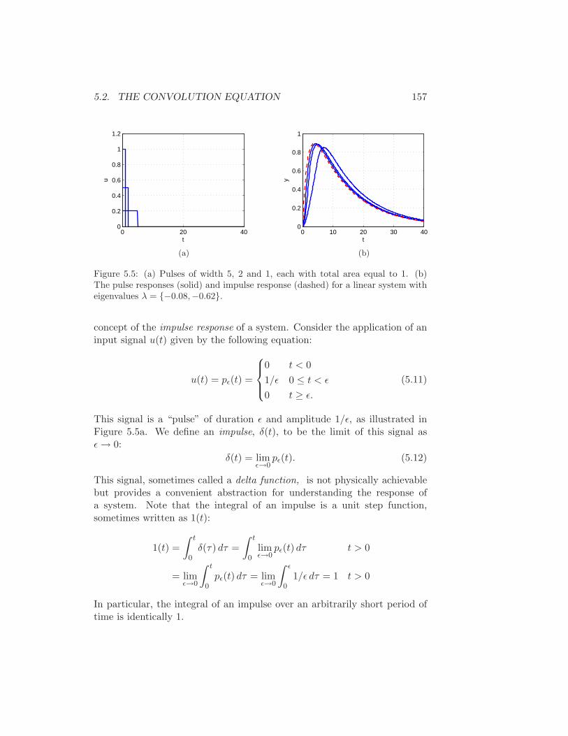
Figure 5.5: (a) Pulses of width 5, 2 and 1, each with total area equal to 1. (b)The pulse responses (solid) and impulse response (dashed) for a linear system witheigenvalues λ = −0.08,−0.62.

concept of the impulse response of a system. Consider the application of aninput signal u(t) given by the following equation:

u(t) = pǫ(t) =

0 t < 0

1/ǫ 0 ≤ t < ǫ

0 t ≥ ǫ.

(5.11)

This signal is a “pulse” of duration ǫ and amplitude 1/ǫ, as illustrated inFigure 5.5a. We define an impulse, δ(t), to be the limit of this signal asǫ→ 0:

δ(t) = limǫ→0

pǫ(t). (5.12)

This signal, sometimes called a delta function, is not physically achievablebut provides a convenient abstraction for understanding the response ofa system. Note that the integral of an impulse is a unit step function,sometimes written as 1(t):

1(t) =

∫ t

0δ(τ) dτ =

∫ t

0limǫ→0

pǫ(t) dτ t > 0

= limǫ→0

∫ t

0pǫ(t) dτ = lim

ǫ→0

∫ ǫ

01/ǫ dτ = 1 t > 0

In particular, the integral of an impulse over an arbitrarily short period oftime is identically 1.


We define the impulse response of a system, h(t), to be the output cor-responding to an impulse as its input:

h(t) =

∫ t

0CeA(t−τ)Bδ(τ) dτ = CeAtB, (5.13)

where the second equality follows from the fact that δ(t) is zero everywhereexcept the origin and its integral is identically one. We can now writethe convolution equation in terms of the initial condition response and theconvolution of the impulse response and the input signal,

y(t) = CeAtx(0) +

∫ t

0h(t− τ)u(τ) dτ. (5.14)

One interpretation of this equation, explored in Exercise 6, is that the re-sponse of the linear system is the superposition of the response to an infiniteset of shifted impulses whose magnitude is given by the input, u(t). Notethat the second term in this equation is identical to equation (5.4) and it canbe shown that the impulse response is formally equivalent to the derivativeof the step response.

The use of pulses as an approximation of the impulse response provides amechanism for identifying the dynamics of a system from data. Figure 5.5bshows the pulse responses of a system for different pulse widths. Notice thatthe pulse responses approaches the impulse response as the pulse width goesto zero. As a general rule, if the fastest eigenvalue of a stable system hasreal part −λmax, then a pulse of length ǫ will provide a good estimate ofthe impulse response if ǫλmax < 1. Note that for Figure 5.5, a pulse widthof ǫ = 1 s gives ǫλmax = 0.62 and the pulse response is very close to theimpulse response.

Coordinate Changes

The components of the input vector u and the output vector y are uniquephysical signals, but the state variables depend on the coordinate systemchosen to represent the state. The choice of coordinates affects the valuesof the matrices A, B and C that are used in the model. (The direct term Dis not affecting since it maps inputs to outputs.) We now investigate someof the consequences of changing coordinate systems.

Introduce new coordinates z by the transformation z = Tx, where T isan invertible matrix. It follows from equation (5.3) that

dz

dt= T (Ax+Bu) = TAT−1z + TBu = Az + Bu

y = Cx+DU = CT−1z +Du = Cz +Du.


The transformed system has the same form as equation (5.3) but the ma-trices A, B and C are different:

A = TAT−1, B = TB, C = CT−1, D = D. (5.15)

As we shall see in several places later in the text, there are often specialchoices of coordinate systems that allow us to see a particular propertyof the system, hence coordinate transformations can be used to gain newinsight into the dynamics.

We can also compare the solution of the system in transformed coordi-nates to that in the original state coordinates. We make use of an importantproperty of the exponential map,

eTST−1

= TeST−1,

which can be verified by substitution in the definition of the exponentialmap. Using this property, it is easy to show that

x(t) = T−1z(t) = T−1eAtTx(0) + T−1

∫ t

0eA(t−τ)Bu(τ) dτ.

From this form of the equation, we see that if it is possible to transformA into a form A for which the matrix exponential is easy to compute, wecan use that computation to solve the general convolution equation for theuntransformed state x by simple matrix multiplications. This technique isillustrated in the next section.

Example 5.5 (Modal form). Suppose that A has n real, distinct eigenval-ues, λ1, . . . , λn. It follows from matrix linear algebra that the correspondingeigenvectors v1, . . . vn are linearly independent and form a basis for R

n. Sup-pose that we transform coordinates according to the rule

x = Mz M =

v1 v2 · · · vn

.

Setting T = M−1, it is easy to show that

A = TAT−1 = M−1AM =

λ1 0λ2

. . .

0 λn

.


b

u(t) = sinωtm m

kk

bq1 q2

k

Figure 5.6: Coupled spring mass system.

To see this, note that if we multiple M−1AM by the basis elements

e1 =

100...0

e2 =

010...0

. . . en =

00...01

we get precisely λiei, which is the same as multiplying the diagonal form bythe canonical basis elements. Since this is true for each ei, i = 1, . . . , n andsince the these vectors form a basis for R

n, the transformed matrix must bein the given form. This is precisely the diagonal form of Example 5.4, whichis also called the modal form for the system. ∇

Example 5.6 (Coupled mass spring system). Consider the coupled massspring system shown in Figure 5.6. The input to this system is the sinusoidalmotion of the end of rightmost spring and the output is the position of eachmass, q1 and q2. The equations of motion for the system are given by

m1q1 = −2kq1 − cq1 + kq2

m2q2 = kq1 − 2kq2 − cq2 + ku

In state-space form, we define the state to be x = (q1, q2, q1, q2) and we canrewrite the equations as

x =

0 0 1 00 0 0 1

−2km

km − c

m 0

km −2k

m 0 − cm

x+

00

0

km

u.

This is a coupled set of four differential equations and quite difficult to solvein analytical form.

5.3. STABILITY AND PERFORMANCE 161

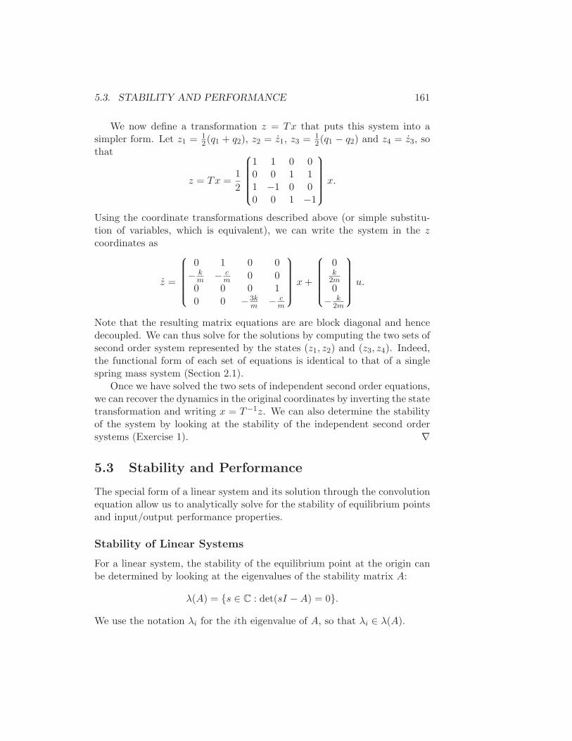
We now define a transformation z = Tx that puts this system into asimpler form. Let z1 = 1

2(q1 + q2), z2 = z1, z3 = 12(q1 − q2) and z4 = z3, so

that

z = Tx =1

2

1 1 0 00 0 1 11 −1 0 00 0 1 −1

x.

Using the coordinate transformations described above (or simple substitu-tion of variables, which is equivalent), we can write the system in the zcoordinates as

z =

0 1 0 0

− km − c

m 0 00 0 0 1

0 0 −3km − c

m

x+

0k

2m0

− k2m

u.

Note that the resulting matrix equations are are block diagonal and hencedecoupled. We can thus solve for the solutions by computing the two sets ofsecond order system represented by the states (z1, z2) and (z3, z4). Indeed,the functional form of each set of equations is identical to that of a singlespring mass system (Section 2.1).

Once we have solved the two sets of independent second order equations,we can recover the dynamics in the original coordinates by inverting the statetransformation and writing x = T−1z. We can also determine the stabilityof the system by looking at the stability of the independent second ordersystems (Exercise 1). ∇

5.3 Stability and Performance

The special form of a linear system and its solution through the convolutionequation allow us to analytically solve for the stability of equilibrium pointsand input/output performance properties.

Stability of Linear Systems

For a linear system, the stability of the equilibrium point at the origin canbe determined by looking at the eigenvalues of the stability matrix A:

λ(A) = s ∈ C : det(sI −A) = 0.

We use the notation λi for the ith eigenvalue of A, so that λi ∈ λ(A).


The easiest class of linear systems to analyze are those whose systemmatrices are in diagonal form. In this case, the dynamics have the form

dx

dt=

λ1 0λ2

. . .

0 λn

x+

β1

β2...βn

u

y =

γ1 γ2 · · · γn

x+Du.

Using Example 5.4, it is easy to show that the state trajectories for thissystem are independent of each other, so that we can write the solution interms of n individual systems

xi = λixi + βiu.

Each of these scalar solutions is of the form

xi(t) = eλitx(0) +

∫ t

0eλ(t−τ)u(t) dt.

If we consider the stability of the system when u = 0, we see that theequilibrium point xe = 0 is stable if λi ≤ 0 and asymptotically stable ifλi < 0.

Very few systems are diagonal, but some systems can be transformedinto diagonal form via coordinate transformations. One such class of sys-tems is those for which the dynamics matrix has distinct (non-repeating)eigenvalues, as outlined in Example 5.5. In this case it is possible to finda matrix T such that the matrix TAT−1 and the transformed system is indiagonal form, with the diagonal elements equal to the the eigenvalues of theoriginal matrix A. We can reason about the stability of the original systemby noting that x(t) = T−1z(t) and so if the transformed system is stable (orasymptotically stable) then the original system has the same type stability.

For more complicated systems, we make use of the following theorem,proved in the next section:

Theorem 5.4. The system

x = Ax

is asymptotically stable if and only if all eigenvalues of A all have strictlynegative real part and is unstable if any eigenvalue of A has strictly positivereal part.


v2

−+

Rb

v1

v3

R1 Ra

R2

C2C1

vo

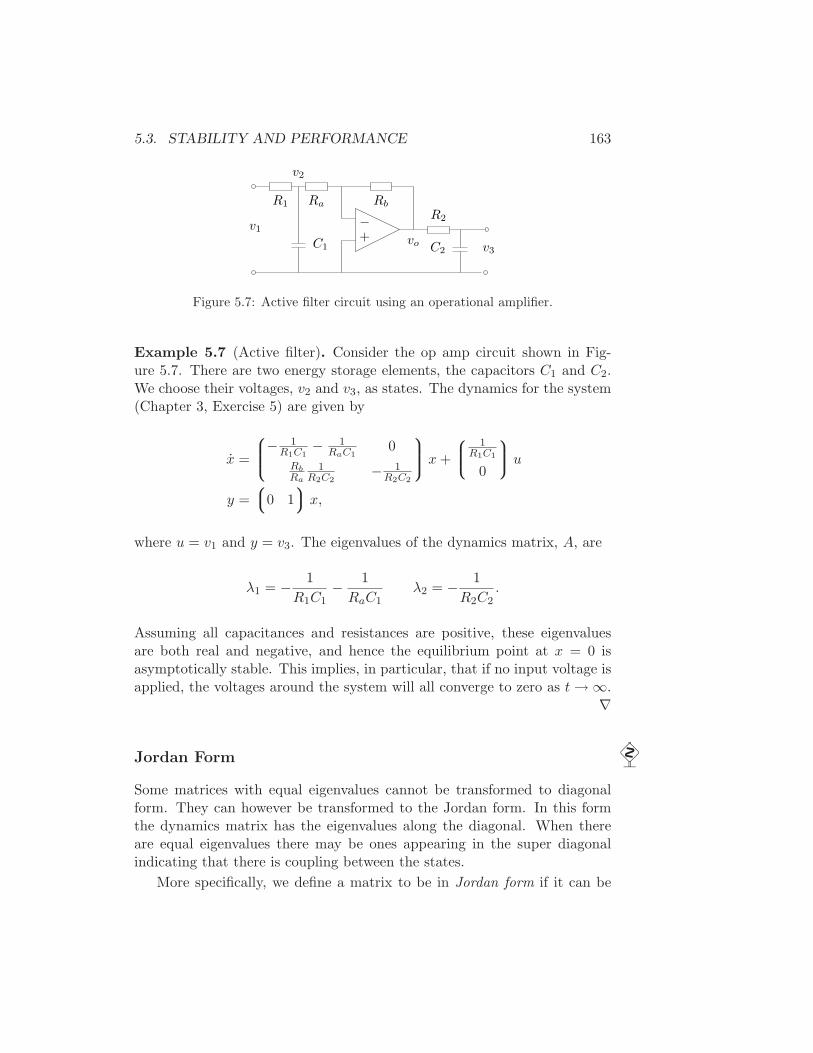
Figure 5.7: Active filter circuit using an operational amplifier.

Example 5.7 (Active filter). Consider the op amp circuit shown in Fig-ure 5.7. There are two energy storage elements, the capacitors C1 and C2.We choose their voltages, v2 and v3, as states. The dynamics for the system(Chapter 3, Exercise 5) are given by

x =

− 1R1C1

− 1RaC1

0

Rb

Ra

1R2C2

− 1R2C2

x+

1R1C1

0

u

y =

0 1

x,

where u = v1 and y = v3. The eigenvalues of the dynamics matrix, A, are

λ1 = − 1

R1C1− 1

RaC1λ2 = − 1

R2C2.

Assuming all capacitances and resistances are positive, these eigenvaluesare both real and negative, and hence the equilibrium point at x = 0 isasymptotically stable. This implies, in particular, that if no input voltage isapplied, the voltages around the system will all converge to zero as t→ ∞.

∇

Jordan Form

Some matrices with equal eigenvalues cannot be transformed to diagonalform. They can however be transformed to the Jordan form. In this formthe dynamics matrix has the eigenvalues along the diagonal. When thereare equal eigenvalues there may be ones appearing in the super diagonalindicating that there is coupling between the states.

More specifically, we define a matrix to be in Jordan form if it can be


written as

J =

J1 0 . . . 00 J2 0

0 . . .. . . 0

0 . . . Jk

where Ji =

λi 1 0 . . . 00 λi 1 0...

. . .. . .

...0 . . . 0 λi 10 . . . 0 0 λi

.

(5.16)Each matrix Ji is called a Jordan block and λi for that block corresponds toan eigenvalue of J .

Theorem 5.5 (Jordan decomposition). Any matrix A ∈ Rn×n can be trans-

formed into Jordan form with the eigenvalues of A determining λi in theJordan form.

Proof. See any standard text on linear algebra, such as Strang [Str88].

Converting a matrix into Jordan form can be very complicated, althoughMATLAB can do this conversion for numerical matrices using the Jordan

function. The structure of the resulting Jordan form is particularly inter-esting since there is no requirement that the individual λi’s be unique, andhence for a given eigenvalue we can have one or more Jordan blocks of dif-ferent size. We say that a Jordan block Ji is trivial if Ji is a scalar (1 × 1block).

Once a matrix is in Jordan form, the exponential of the matrix can becomputed in terms of the Jordan blocks:

eJ =

eJ1 0 . . . 00 eJ2 0

0 . . .. . . 0

0 . . . eJk .

(5.17)

This follows from the block diagonal form of J . The exponentials of theJordan blocks can in turn be written as

eJit =

eλit t eλit t2

2! eλit . . . tn−1

(n−1)! eλit

0 eλit t eλit . . . tn−2

(n−2)! eλit

eλit. . .. . . t eλit

0 eλit

(5.18)


When there are multiple eigenvalues, the invariant subspaces represent-ing the modes correspond to the Jordan blocks of the matrix A . Note that λmay be complex, in which case the transformation T that converts a matrixinto Jordan form will also be complex. When λ has a non-zero imaginarycomponent, the solutions will have oscillatory components since

eσ+jωt = eσt(cosωt+ j sinωt).

We can now use these results to prove Theorem 5.4.

Proof of Theorem 5.4. Let T ∈ Cn×n be an invertible matrix that trans-

forms A into Jordan form, J = TAT−1. Using coordinates z = Tx, we canwrite the solution z(t) as

z(t) = eJtz(0).

Since any solution x(t) can be written in terms of a solution z(t) with z(0) =Tx(0), it follows that it is sufficient to prove the theorem in the transformedcoordinates.

The solution z(t) can be written as a combination of the elements ofthe matrix exponential and from equation (5.18) these elements all decayto zero for arbitrary z(0) if and only if Reλi < 0. Furthermore, if any λi

has positive real part, then there exists an initial condition z(0) such thatthe corresponding solution increases without bound. Since we can scale thisinitial condition to be arbitrarily small, it follows that the equilibrium pointis unstable if any eigenvalue has positive real part.

The existence of a canonical form allows us to prove many properties oflinear systems by changing to a set of coordinates in which the A matrix isin Jordan form. We illustrate this in the following proposition, which followsalong the same lines as the proof of Theorem 5.4.

Proposition 5.6. Suppose that the system

x = Ax

has no eigenvalues with strictly positive real part and one or more eigenval-ues with zero real part. Then the system is stable if and only if the Jordanblocks corresponding to each eigenvalue with zero real part are scalar (1× 1)blocks.

Proof. Exercise 3.


Input/Output Response

So far, this chapter has focused on the stability characteristics of a system.While stability is often a desirably feature, stability alone may not be suf-ficient in many applications. We will want to create feedback systems thatquickly react to changes and give high performance in measurable ways.

We return now to the case of an input/output state space system

dx

dt= Ax+Bu

y = Cx+Du,(5.19)

where x ∈ Rn is the state and u, y ∈ R are the input and output. The

general form of the solution to equation (5.19) is given by the convolutionequation:

y(t) = CeAtx(0) +

∫ t

0CeA(t−τ)Bu(τ)dτ +Du(t).

We see from the form of this equation that the solution consists of an initialcondition response and an input response.

The input response, corresponding to the second term in the equationabove, itself consists of two components—the transient response and steadystate response. The transient response occurs in the first period of time afterthe input is applied and reflects the mismatch between the initial conditionand the steady state solution. The steady state response is the portion ofthe output response that reflects the long term behavior of the system underthe given inputs. For inputs that are periodic, the steady state response willoften also be periodic. An example of the transient and steady state responseis shown in Figure 5.8.

Step Response

A particularly common form of input is a step input, which represents anabrupt change in input from one value to another. A unit step is defined as

u = 1(t) =

0 t = 0

1 t > 0.

The step response of the system (5.3) is defined as the output y(t) startingfrom zero initial condition (or the appropriate equilibrium point) and givena step input. We note that the step input is discontinuous and hence is not


0 10 20 30 40 50 60 70 80−1

−0.5

0

0.5

1

inpu

t, u(

t)

0 10 20 30 40 50 60 70 80−0.1

−0.05

0

0.05

0.1

time (sec)

outp

ut, y

(t)

Input

Output

Steady StateTransient

Figure 5.8: Transient versus steady state response. The top plot shows the input toa linear system and the bottom plot the corresponding output. The output signalinitially undergoes a transient before settling into its steady state behavior.

physically implementable. However, it is a convenient abstraction that iswidely used in studying input/output systems.

We can compute the step response to a linear system using the convo-lution equation. Setting x(0) = 0 and using the definition of the step inputabove, we have

y(t) =

∫ t

0CeA(t−τ)Bu(τ)dτ +Du(t)

=

∫ t

0CeA(t−τ)Bdτ +D t > 0.

If A has eigenvalues with negative real part (implying that the origin is astable equilibrium point in the absence of any input), then we can rewritethe solution as

y(t) = CA−1eAtB︸︷︷︸

transient

+D − CA−1B︸︷︷︸

steady state

t > 0. (5.20)


0 5 10 15 20 25 300

0.5

1

1.5

2

time (sec)

Out

put

Rise time

Settling time

Overshoot

Steady state value

Figure 5.9: Sample step response

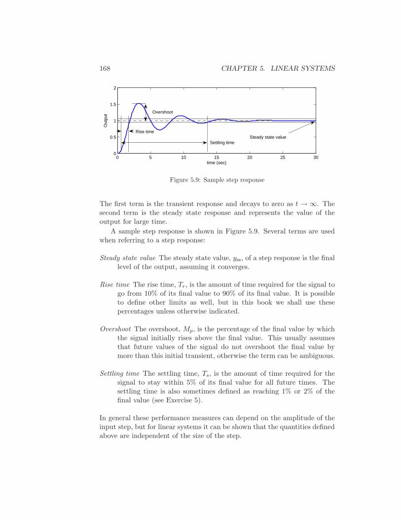
The first term is the transient response and decays to zero as t → ∞. Thesecond term is the steady state response and represents the value of theoutput for large time.

A sample step response is shown in Figure 5.9. Several terms are usedwhen referring to a step response:

Steady state value The steady state value, yss, of a step response is the finallevel of the output, assuming it converges.

Rise time The rise time, Tr, is the amount of time required for the signal togo from 10% of its final value to 90% of its final value. It is possibleto define other limits as well, but in this book we shall use thesepercentages unless otherwise indicated.

Overshoot The overshoot, Mp, is the percentage of the final value by whichthe signal initially rises above the final value. This usually assumesthat future values of the signal do not overshoot the final value bymore than this initial transient, otherwise the term can be ambiguous.

Settling time The settling time, Ts, is the amount of time required for thesignal to stay within 5% of its final value for all future times. Thesettling time is also sometimes defined as reaching 1% or 2% of thefinal value (see Exercise 5).

In general these performance measures can depend on the amplitude of theinput step, but for linear systems it can be shown that the quantities definedabove are independent of the size of the step.


Frequency Response

The frequency response of an input/output system measures the way inwhich the system responds to a sinusoidal excitation on one of its inputs.As we have already seen for linear systems, the particular solution associatedwith a sinusoidal excitation is itself a sinusoid at the same frequency. Hencewe can compare the magnitude and phase of the output sinusoid to theinput. More generally, if a system has a sinusoidal output response at thesame frequency as the input forcing, we can speak of the frequency responseof the system.

To see this in more detail, we must evaluate the convolution equa-tion (5.10) for u = cosωt. This turns out to be a very messy computation,but we can make use of the fact that the system is linear to simplify thederivation. In particular, we note that

cosωt =1

2

(

ejωt + e−jωt)

.

Since the system is linear, it suffices to compute the response of the systemto the complex input u(t) = est and we can always reconstruct the input to asinusoid by averaging the responses corresponding to s = jωt and s = −jωt.

Applying the convolution equation to the input u = est, we have

y(t) =

∫ t

0CeA(t−τ)Besτdτ +Dest

=

∫ t

0CeA(t−τ)+sIτBdτ +Dest

= eAt

∫ t

0Ce(sI−A)τBdτ +Dest.

If we assume that none of the eigenvalues of A are equal to s = ±jω, thenthe matrix sI −A is invertible and we can write (after some algebra)

y(t) = CeAt(

x(0) − (sI −A)−1B)

︸︷︷︸

transient

+(

D + C(sI −A)−1B)

est

︸︷︷︸

steady state

.

Notice that once again the solution consists of both a transient componentand a steady state component. The transient component decays to zeroif the system is asymptotically stable and the steady state component isproportional to the (complex) input u = est.


0 5 10 15 20 25 30−1.5

−1

−0.5

0

0.5

1

1.5

time (sec)

Inpu

t, O

utpu

t

Au

Ay

∆T

T

input output

Figure 5.10: Frequency response, showing gain and phase. The phase lag is givenby θ = −2π∆T/T .

We can simplify the form of the solution slightly further by rewriting thesteady state response as

yss = Mejθest = Me(st+jθ)

whereMejθ = C(sI −A)−1B +D (5.21)

and M and θ represent the magnitude and phase of the complex numberD + C(sI − A)−1B. When s = jω, we say that M is the gain and θ isthe phase of the system at a given forcing frequency ω. Using linearity andcombining the solutions for s = +jω and s = −jω, we can show that if wehave an input u = Au sin(ωt+ ψ) and output y = Ay sin(ωt+ ϕ), then

gain(ω) =Ay

Au= M phase(ω) = ϕ− ψ = θ.

If the phase is positive, we say that the output “leads” the input, otherwisewe say it “lags” the input.

A sample frequency response is illustrated in Figure 5.10. The solidline shows the input sinusoid, which has amplitude 1. The output sinusoidis shown as a dashed line, and has a different amplitude plus a shiftedphase. The gain is the ratio of the amplitudes of the sinusoids, which can bedetermined by measuring the height of the peaks. The phase is determinedby comparing the ratio of the time between zero crossings of the input andoutput to the overall period of the sinusoid:

θ = −2π · δTT.


10−1

100

101

102

103

104

10−6

10−4

10−2

100

102

Gai

n

10−1

100

101

102

103

104

−150

−100

−50

0

Pha

se (

deg)

Frequency (rad/sec)

Figure 5.11: Frequency response for the active filter from Example 5.7. The upperplot shows the magnitude as a function of frequency (on a log-log scale) and thelower plot shows the phase (on a log-linear scale).

Example 5.8 (Active filter). Consider the active filter presented in Ex-ample 5.7. The frequency response for the system can be computed usingequation (5.21):

Mejθ = C(sI −A)−1B +D =Rb/Ra

(1 +R2C2s)(R1+Ra

Ra+R1C1s)

s = jω.

The magnitude and phase are plotted in Figure 5.11 for Ra = 1kΩ, Rb =100 kΩ, R1 = 100Ω, R2 = 5kΩ and C1 = C2 = 100 µF. ∇

The gain at frequency ω = 0 is called the zero frequency gain of thesystem and corresponds to the ratio between a constant input and the steadyoutput:

M0 = CA−1B +D.

Note that the zero frequency gain is only well defined if A is invertible (and,in particular, if it does has not eigenvalues at 0). It is also important to notethat the zero frequency gain is only a relevant quantity when a system is


stable about the corresponding equilibrium point. So, if we apply a constantinput u = r then the corresponding equilibrium point

xe = −A−1Br

must be stable in order to talk about the zero frequency gain. (In electricalengineering, the zero frequency gain is often called the “DC gain”. DCstands for “direct current” and reflects the common separation of signalsin electrical engineering into a direct current (zero frequency) term and analternating current (AC) term.)

5.4 Second Order Systems

One class of systems that occurs frequently in the analysis and design offeedback systems is second order, linear differential equations. Because oftheir ubiquitous nature, it is useful to apply the concepts of this chapter tothat specific class of systems and build more intuition about the relationshipbetween stability and performance.

The canonical second order system is a differential equation of the form

q + 2ζω0q + ω20q = ku

y = q.(5.22)

In state space form, this system can be represented as

x =

0 1

−ω20 −2ζω0

x+

0k

u

y =

1 0

x

(5.23)

The eigenvalues of this system are given by

λ = −ζω0 ±√

ω20(ζ

2 − 1)

and we see that the origin is a stable equilibrium point if ω0 > 0 andζ > 0. Note that the eigenvalues are complex if ζ < 1 and real otherwise.Equations (5.22) and (5.23) can be used to describe many second ordersystems, including a damped spring mass system and an active filter, asshown in the examples below.

The form of the solution depends on the value of ζ, which is referred toas the damping factor for the system. If ζ > 1, we say that the system is

5.4. SECOND ORDER SYSTEMS 173

overdamped and the natural response (u = 0) of the system is given by

y(t) =βx10 + x20

β − αe−αt − αx10 + x20

β − αe−βt

where α = ω0(ζ +√

ζ2 − 1) and β = ω0(ζ −√

ζ2 − 1). We see that theresponse consists of the sum of two exponentially decaying signals. If ζ = 1then the system is critically damped and solution becomes

y(t) = e−ζω0t(x10 + (x20 + ζω0x10)t

).

Note that this is still asymptotically stable as long as ω0 > 0, although thesecond term in the solution is increasing with time (but more slowly thanthe decaying exponential that multiplies it).

Finally, if 0 < ζ < 1, then the solution is oscillatory and equation (5.22)is said to be underdamped. The parameter ω0 is referred to as the naturalfrequency of the system, stemming from the fact that for small ζ, the eigen-values of the system are approximately λ = −ζ± jω0. The natural responseof the system is given by

y(t) = e−ζω0t

(

x10 cosωdt+(ζω0

ωdx10 +

1

ωdx20

)

sinωdt

)

,

where ωd = ω0

√

1 − ζ2. For ζ ≪ 1, ωd ≈ ω0 defines the oscillation frequencyof the solution and ζ gives the damping rate relative to ω0.

Because of the simple form of a second order system, it is possible tosolve for the step and frequency responses in analytical form. The solutionfor the step response depends on the magnitude of ζ:

y(t) =k

ω20

(

1 − e−ζω0t cosωdt+ζ

√

1 − ζ2e−ζω0t sinωdt

)

ζ < 1

y(t) =k

ω20

(1 − e−ω0t(1 + ω0t)

)ζ = 1

y(t) =k

ω20

(

1 − e−ω0t − 1

2(1 + ζ)eω0(1−2ζ)t

)

ζ > 1,

(5.24)where we have taken x(0) = 0. Note that for the lightly damped case(ζ < 1) we have an oscillatory solution at frequency ωd, sometimes calledthe damped frequency.

The step responses of systems with k = ω2 and different values of ζ areshown in Figure 5.12, using a scaled time axis to allow an easier comparison.


0 5 10 150

0.5

1

1.5

2

ω0t

y

ζ

Figure 5.12: Normalized step responses h for the system (5.23) for ζ = 0 (dashed),0.1, 0.2, 0.5, 0.707 (dash dotted), 1, 2, 5 and 10 (dotted).

The shape of the response is determined by ζ and the speed of the responseis determined by ω0 (including in the time axis scaling): the response isfaster if ω0 is larger. The step responses have an overshoot of

Mp =

e−πζ/√

1−ζ2

for |ζ| < 1

0 for ζ ≥ 1.(5.25)

For ζ < 1 the maximum overshoot occurs at

tmax =π

ω0

√

1 − ζ2. (5.26)

The maximum decreases and is shifted to the right when ζ increases and itbecomes infinite for ζ = 1, when the overshoot disappears.

The frequency response can also be computed explicitly and is given by

Mejθ =ω2

0

(jω)2 + 2ζω0(jω) + ω20

=ω2

0

ω20 − ω2 + 2jζω0ω

.

A graphical illustration of the frequency response is given in Figure 5.13.Notice the resonance peak that increases with decreasing ζ. The peak isoften characterized by is Q-value, defined as Q = 1/2ζ.

Example 5.9 (Damped spring mass). The dynamics for a damped springmass system are given by

mq + cq + kq = u,

where m is the mass, q is the displacement of the mass, c is the coefficientof viscous friction, k is the spring constant and u is the applied force. We

5.4. SECOND ORDER SYSTEMS 175

10−1

100

101

10−2

10−1

100

101

10−1

100

101

−150

−100

−50

0

ζ

ζ

Figure 5.13: Frequency response of a the second order system (5.23). The uppercurve shows the gain ratio, M , and the lower curve shows the phase shift, θ. Theparameters is Bode plot of the system with ζ = 0 (dashed), 0.1, 0.2, 0.5, 0.7 and1.0 (dashed-dot).

can convert this into the standard second order for by dividing through bym, giving

q +c

mq +

k

mq =

1

mu.

Thus we see that the spring mass system has natural frequency and dampingratio given by

ω0 =

√

k

mζ =

c

2√km

(note that we have use the symbol k for the stiffness here; it should not beconfused with the gain term in equation (5.22)). ∇

One of the other reasons why second order systems play such an important role in feedback systems is that even for more complicated systems theresponse is often dominated by the “dominant eigenvalues”. To define thesemore precisely, consider a system with eigenvalues λi, i = 1, . . . , n. We


define the damping factor for a complex eigenvalue λ to be

ζ =−Reλ

|λ|

We say that a complex conjugate pair of eigenvalues λ, λ∗ is a dominantpair if it has the lowest damping factor compared with all other eigenvaluesof the system.

Assuming that a system is stable, the dominant pair of eigenvalues tendsto be the most important element of the response. To see this, assume thatwe have a system in Jordan form with a simple Jordan block correspondingto the dominant pair of eigenvalues:

z =

λλ∗

J2

. . .

Jk

z +Bu

y = Cz.

(Note that the state z may be complex due to the Jordan transformation.)The response of the system will be a linear combination of the responsesfrom each of the individual Jordan subsystems. As we see from Figure 5.12,for ζ < 1 the subsystem with the slowest response is precisely the one withthe smallest damping factor. Hence when we add the responses from eachof the individual subsystems, it is the dominant pair of eigenvalues that willbe dominant factor after the initial transients due to the other terms in thesolution. While this simple analysis does not always hold (for example, ifsome non-dominant terms have large coefficients due to the particular formof the system), it is often the case that the dominant eigenvalues dominatethe (step) response of the system. The following example illustrates theconcept.

5.5 Linearization

As described in the beginning of the chapter, a common source of linearsystem models is through the approximation of a nonlinear system by a linearone. These approximations are aimed at studying the local behavior of asystem, where the nonlinear effects are expected to be small. In this sectionwe discuss how to locally approximate a system by its linearization and what

5.5. LINEARIZATION 177

can be said about the approximation in terms of stability. We begin withan illustration of the basic concept using the speed control example fromChapter 2.

Example 5.10 (Cruise control). The dynamics for the cruise control systemare derived in Section 3.1 and have the form

mdv

dt= αnuT (αnv) −mgCr − 1

2ρCvAv2 −mg sin θ, (5.27)

where the first term on the right hand side of the equation is the force gen-erated by the engine and the remaining three terms are the rolling friction,aerodynamic drag and gravitational disturbance force. There is an equilib-rium (ve, ue) when the force applied by the engine balances the disturbanceforces.

To explore the behavior of the system near the equilibrium we will lin-earize the system. A Taylor series expansion of equation (5.27) around theequilibrium gives

d(v − ve)

dt= a(v − ve) − bg(θ − θe) + b(u− ue) (5.28)

where

a =ueα

2nT

′(αnve) − ρCvAve

mbg = g cos θe b =

αnT (αnve)

m(5.29)

and terms of second and higher order have been neglected. For a car infourth gear with ve = 25 m/s, θe = 0 and the numerical values for the carfrom Section 3.1, the equilibrium value for the throttle is ue = 0.1687 andthe model becomes

d(v − ve)

dt= −0.0101(v − ve) + 1.3203(u− ue) − 9.8(θ − θe) (5.30)

This linear model describes how small perturbations in the velocity aboutthe nominal speed evolve in time.

Figure 5.14, which shows a simulation of a cruise controller with linearand nonlinear models, indicates that the differences between the linear andnonlinear models is not visible in the graph. ∇

Linear Approximation

To proceed more formally, consider a single input, single output nonlinearsystem

dx

dt= f(x, u) x ∈ R

n, u ∈ R

y = h(x, u) y ∈ R

(5.31)


0 5 10 15 20 25 30

19

19.5

20

20.5

0 5 10 15 20 25 300

0.5

1

Thro

ttle

Vel

oci

ty[m

/s]

Time [s]

Figure 5.14: Simulated response of a vehicle with PI cruise control as it climbs ahill with a slope of 4. The full lines is the simulation based on a nonlinear modeland the dashed line shows the corresponding simulation using a linear model. Thecontroller gains are kp = 0.5 and ki = 0.1.

with an equilibrium point at x = xe, u = ue. Without loss of generality,we assume that xe = 0 and ue = 0, although initially we will consider thegeneral case to make the shift of coordinates explicit.

In order to study the local behavior of the system around the equilib-rium point (xe, ue), we suppose that x − xe and u − ue are both small, sothat nonlinear perturbations around this equilibrium point can be ignoredcompared with the (lower order) linear terms. This is roughly the same typeof argument that is used when we do small angle approximations, replacingsin θ with θ and cos θ with 1 for θ near zero.

In order to formalize this idea, we define a new set of state variables z,inputs v, and outputs w:

z = x− xe v = u− ue w = y − h(xe, ue).

These variables are all close to zero when we are near the equilibrium point,and so in these variables the nonlinear terms can be thought of as the higherorder terms in a Taylor series expansion of the relevant vector fields (assum-ing for now that these exist).

Example 5.11. Consider a simple scalar system,

x = 1 − x3 + u.


The point (xe, ue) = (1, 0) is an equilibrium point for this system and wecan thus set

z = x− 1 v = u.

We can now compute the equations in these new coordinates as

z =d

dt(x− 1) = x

= 1 − x3 + u = 1 − (z + 1)3 + v

= 1 − z3 − 3z2 − 3z − 1 + v = −3z − 3z2 − z3 + v.

If we now assume that x stays very close to the equilibrium point, thenz = x− xe is small and z ≪ z2 ≪ z3. We can thus approximate our systemby a new system

z = −3z + v.

This set of equations should give behavior that is close to that of the originalsystem as long as z remains small. ∇

More formally, we define the Jacobian linearization of the nonlinear sys-tem (5.31) as

z = Az +Bv

w = Cz +Dv,(5.32)

where

A =∂f(x, u)

∂x

∣∣∣∣(xe,ue)

B =∂f(x, u)

∂u

∣∣∣∣(xe,ue)

C =∂h(x, u)

∂x

∣∣∣∣(xe,ue)

D =∂h(x, u)

∂u

∣∣∣∣(xe,ue)

(5.33)

The system (5.32) approximates the original system (5.31) when we are nearthe equilibrium point that the system was linearized about.

It is important to note that we can only define the linearization of a sys-tem about an equilibrium point. To see this, consider a polynomial system

x = a0 + a1x+ a2x2 + a3x

3 + u,

where a1 6= 0. There are a family of equilibrium points for this system givenby (xe, ue) = (xe,−a0−a1xe−a2x

2e −a3x

3e) and we can linearize around any

of these. Suppose that we try to linearize around the origin of the system,x = 0, u = 0. If we drop the higher order terms in x, then we get

x = a0 + a1x+ u,


which is not the Jacobian linearization if a0 6= 0. The constant term mustbe kept and this is not present in (5.32). Furthermore, even if we kept theconstant term in the approximate model, the system would quickly moveaway from this point (since it is “driven” by the constant term a0) andhence the approximation could soon fail to hold.

Software for modeling and simulation frequently has facilities for per-forming linearization symbolically or numerically. The MATLAB commandtrim finds the equilibrium and linmod extracts linear state-space modelsfrom a SIMULINK system around an operating point.

Example 5.12 (Vehicle steering). Consider the vehicle steering system in-troduced in Section 2.8. The nonlinear equations of motion for the systemare given by equations (2.21)–(2.23) and can be written as

d

dt

xyθ

=

v0cos (α+θ)

cos α

v0sin (α+θ)

cos α

v0

b tan δ

,

where x, y and θ are the position and orientation of the center of mass ofthe vehicle, v0 is the velocity of the rear wheel, δ is the angle of the frontwheel and α is the anglular devitation of the center of mass from the rearwheel along the instantaneous circle of curvature determined by the frontwheel:

α(δ) = arctan(a tan δ

b

)

.

We are interested in the motion of the vehicle about a straight line path(θ = θ0) with fixed velocity v0 6= 0. To find the relevant equilibrium point,we first set θ = 0 and we see that we must have δ = 0, corresponding to thesteering wheel being straight. This also yields α = 0. Looking at the firsttwo equations in the dynamics, we see that the motion in the xy directionis by definition not at equilibrium since x2 + y2 = v2

0 6= 0. Therefore wecannot formally linearize the full model.

Suppose instead that we are concerned with the lateral deviation of thevehicle from a straight line. For simplicity, we let θ0 = 0, which correspondsto driving along the x axis. We can then focus on the equations of motionin the y and θ directions, for which we have

d

dt

yθ

=

v0sin (α+θ)

cos α

v0

b tan δ

.


Abusing notation, we write x = (y, θ) and u = δ so that

f(x, u) =

v0sin(α(u)+x2)

cos α(u)v0

b tanu,

where the equilibrium point of interest is now given by x = (0, 0) and u = 0.To compute the linearization the model around the equilibrium point,

we make use of the formulas (5.33). A straightforward calculation yields

A =∂f(x, u)

∂x

∣∣∣∣x=0u=0

=

0 v00 0

δ B =∂f(x, u)

∂u

∣∣∣∣x=0u=0

=

v0ab

v0

b

and the linearized systemz = Az +Bv (5.34)

thus provides an approximation to the original nonlinear dynamics.A model can often be simplified further by introducing normalized di-

mension free variables. For this system, we can normalize lengths by thewheel base b and introduce a new time variable τ = v0t/b. The time unit isthus the time is takes for the vehicle to travel one wheel base. We similarlynormalize the lateral position and write w1 = y/b, w2 = θ. The model (5.34)then becomes

dw

dτ=

w2 + αv

v

=

0 10 0

w +

α1

v

y =

1 0

w

(5.35)

The normalized linear model for vehicle steering with non-slipping wheels isthus a linear system with only one parameter α = a/b. ∇

Feedback Linearization

Another type of linearization is the use of feedback to convert the dynamicsof a nonlinear system into a linear one. We illustrate the basic idea with anexample.

Example 5.13 (Cruise control). Consider again the cruise control systemfrom Example 5.10, whose dynamics is given in equation (5.27). If we chooseu as a feedback law of the form

u =1

αnT (αnv)

(

u′ +mgCr +1

2ρCvAv

2

)

(5.36)


then the resulting dynamics become

mdv

dt= u′ + d (5.37)

where d = mg sin θ is the disturbance force due the slope of the road. Ifwe now define a feedback law for u′ (such as a PID controller), we can useequation (5.36) to compute the final input that should be commanded.

Equation (5.37) is a linear differential equation. We have essentially“inverted out” the nonlinearity through the use of the feedback law (5.36).This requires that we have an accurate measurement of the vehicle velocityv as well as an accurate model of the torque characteristics of the engine,gear ratios, drag and friction characteristics and mass of the car. While sucha model is not generally available (remembering that the parameter valuescan change), if we design a good feedback law for u′, then we can achieverobustness to these uncertainties. ∇

More generally, we say that a system of the form

dx

dt= f(x, u)

y = h(x)

is feedback linearizable if we can find a control law u = α(x, v) such thatthe resulting closed loop system is input/output linear with input v andoutput u. To fully characterize such systems is beyond the scope of thistext, but we note that in addition to changes in the input, we must alsoallow for (nonlinear) changes in the states that are used to describe thesystem, keeping only the input and output variables fixed. More detailsof this process can be found in the the textbooks by Isidori [Isi89] andKhalil [Kha92].

One case the comes up relatively frequently, and is hence worth specialmention, is the set of mechanical systems of the form

M(q)q + C(q, q)q +N(q, q) = B(q)u.

Here q ∈ Rn is the configuration of the mechanical system, M(q) ∈ R

n×n

is the configuration-dependent inertia matrix, C(q, q)q ∈ Rn represents the

Coriolis forces, N(q, q) ∈ Rn are additional nonlinear forces (such as stiffness

and friction) and B(q) ∈ Rn×p is the input matrix. If p = n then we have

the same number of inputs and configuration variables and if we further

5.6. FURTHER READING 183

have that B(q) is an invertible matrix for all configurations q, then we canchoose

u = B−1(q) (M(q)v − C(q, q)q −N(q, q)) . (5.38)

The resulting dynamics become

M(q)q = M(q)v =⇒ q = v,

which is a linear system. We can now use the tools of linear systems theoryto analyze and design control laws for the linearized system, rememberingto apply equation (5.38) to obtain the actual input that will be applied tothe system.

This type of control is common in robotics, where it goes by the nameof computed torque, and aircraft flight control, where it is called dynamicinversion.

Local Stability of Nonlinear Systems

Having constructed a linearized model around an equilibrium point, we cannow ask to what extent this model predicts the behavior of the originalnonlinear system. The following theorem gives a partial answer for the caseof stability.

Theorem 5.7. Consider the system (5.31) and let A ∈ Rn×n be defined as

in equations (5.32) and (5.33). If the real part of the eigenvalues of A arestrictly less than zero, then xe is a locally asymptotically stable equilibriumpoint of (5.31).

This theorem shows that global asymptotic stability of the linearizationimplies local asymptotic stability of the original nonlinear system. The esti-mates provided by the proof of the theorem can be used to give a (conserva-tive) bound on the domain of attraction of the origin. Systematic techniquesfor estimating the bounds on the regions of attraction of equilibrium pointsof nonlinear systems is an important area of research and involves searchingfor the “best” Lyapunov functions.

The proof of this theorem is the beyond the scope of this text, but canbe found in [Kha92].

5.6 Further Reading

The idea to characterize dynamics by considering the responses to step in-puts is due to Heaviside. The unit step is therefore also called the Heaviside


step function. The majority of the material in this chapter is very classicaland can be found in most books on dynamics and control theory, includ-ing early works on control such as James, Nichols and Phillips [JNP47], andmore recent textbooks such as Franklin, Powell and Emami-Naeni [FPEN05]and Ogata [Oga01]. The material on feedback linearization is typically pre-sented in books on nonlinear control theory, such as Khalil [Kha92]. Tracermethods are described in [She62].

5.7 Exercises

1. Compute the full solution to the couple spring mass system in Ex-ample 5.6 by transforming the solution for the block diagonal systemback into the original set of coordinates. Show that the system isasymptotically stable if m, b and k are all greater than zero.

2. Using the computation for the matrix exponential, show that equa-tion (5.18) holds for the case of a 3×3 Jordan block. (Hint: decomposethe matrix into the form S +N where S is a diagonal matrix.)

3. Prove Proposition 5.6.

4. Show that the step response for an asymptotically stable linear systemis given by equation (5.20).

5. Consider a first order system of the form

x = −τx+ u

y = x.

We say that the parameter τ is the time constant for the system sincethe zero input system approaches the origin as eτt. For a first ordersystem of this form, show that the rise time of the system is approxi-mately 2τ , a 5% settling time corresponds to approximately 3τ and a2% settling time corresponds to approximately 4τ .

6. Show that a signal u(t) can be decomposed in terms of the impulsefunction δ(t) as

u(t) =

∫ t

0δ(t− τ)u(τ) dτ

and use this decomposition plus the principle of superposition to showthat the response of a linear system to an input u(t) (assuming zero

5.7. EXERCISES 185

initial condition) can be written as

y(t) =

∫ t

0h(t− τ)u(τ) dτ,

where h(t) is the impulse response of the system.

7. Consider a linear discrete time system of the form

xk+1 = Axk +Buk

yk = Cxk +Duk.

(a) Show that the general form of the output of a discrete time linearsystem is given by the discrete time convolution equation:

yk = CAkx0 +k∑

i=0

CAiBui +Duk

(b) Show that a discrete time linear system is asymptotically stable ifand only if all eigenvalues of A have magnitude strictly less than1.

(c) Let uk = A sin(ωk) represent an oscillatory input with frequencyω < π (to avoid “aliasing”). Show that the steady state compo-nent of the response has gain M and phase θ where

Mejθ = C(jωI −A)−1B +D.

(d) Show that if we have a nonlinear discrete time system

xk = f(xk, uk) xk ∈ Rn, u ∈ R

yk = h(xk, u)k) y ∈ R

then we can linearize the system around an equilibrium point(xe, ue) by defining the matrices A, B, C and D as in equa-tion (5.33).

8. Consider the consensus protocol introduced in Example 2.13. Showthat if the connectivity graph of the sensor network is connected, thenwe can find a gain γ such that the agent states converge to the averagevalue of the measure quantity.

linear systems - dynamical systemsmurray/books/am05/pdf/am06-linsys_16sep06.… · linear systems...

Documents