linear system theory - wordpress.com · why study linear systems? i linear system is a special case...
TRANSCRIPT

Linear System Theory
Wonhee KimLecture 1
March 7, 2017
1 / 22

Overview
I Course Information
I Prerequisites
I Course Outline
I What is Control Engineering?
I Examples of Control Systems
I Structure of Control Systems
I Linear Systems
I Nonlinear Systems
2 / 22

Course Information
I Instructor: Wonhee Kim
I Email/Office: [email protected]/Room 310-439
I Course Website: wonheekim.wordpress.com
I Textbook: Chi-Tsong Chen, Linear System Theory, 4th edition,Oxford University Press, available at the UNIST bookstore
I Grading Policy: HW(20%), Midterm(40%), Final Exam (40%)
I Check the course website for updates
I Original lecture note supported by Prof. Jun Moon (UNIST)
3 / 22

Prerequisites
I linear algebra
I signals and systems: Laplace transform (z-transform)
I differential and difference equations
I some familiarity of classical control theory (Bode plot, root locus,Nyquist, PID, etc) and programming skills (e.g. MATLAB) would behelpful
I We will cover the required mathematical skills during the lectures
4 / 22

Tentative Course Topics
I linear algebraI vector space, norm, inner product, column and null spaces,
eigenvalues, basis, rank, similarity transformation, Jordan form, etc.
I ordinary differential equations (and difference equations)I state space representation, solutions, matrix exponential, etc
I stability
I controllability, observability, decomposition
I linear system designI state-feedback, pole-placement, observer design
I optimal control (if time permits)
5 / 22

What is Control Engineering?
I Control Engineering (Wikipedia): Control engineering is theengineering discipline that applies control theory to design systemswith desired behaviors.
I Control Theory (Wikipedia): Control theory is an interdisciplinarybranch of engineering and mathematics that deals with the behaviorof dynamical systems with inputs, and how their behavior ismodified by feedback.
I In this course, we will study mathematical control theory
6 / 22

Examples of Control Systems
I Aircraft, Vehicles, Defense, Circuits, Communication, PowerSystems, Social Networks, Economics, etc
I Desired behavior: safety, speed, position, price, power, etc.
7 / 22

Examples of Control SystemsI Segway: https://www.youtube.com/watch?v=rmlg5QkusFQ
(control of an inverted pendulum)
I HDD: control of spindle and actuator (sensor) motors
8 / 22
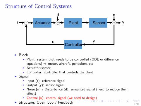
Structure of Control Systems
Plant SensorActuator +-
Controller
d
+
n
u
r
y
y
I BlockI Plant: system that needs to be controlled (ODE or difference
equations) ⇒ motor, aircraft, pendulum, etcI Actuator/sensorI Controller: controller that controls the plant
I SignalI Input (r): reference signalI Output (y): sensor signalI Noise (n) / Disturbance (d): unwanted signal (need to reduce their
effect)I Control (u): control signal (we need to design)
I Structure: Open loop / Feedback9 / 22

Continuous-Time Linear Time-Varying (LTV) System
x(t) =dx(t)
dt= A(t)x(t) + B(t)u(t) + D(t)d(t)
y(t) = C (t)x(t) + E (t)u(t) + F (t)n(t)
I t ≥ 0: timeI x ∈ Rn: stateI u ∈ Rm: controlI d ∈ Rl : disturbanceI y ∈ Rp: (sensor) outputI n ∈ Rq: noiseI A(t): n × n system matrixI B(t): n ×m input matrixI D(t): n × l disturbance matrixI C (t): p × n output matrixI E (t): p ×m feedthrough matrixI F (t): p × q noise matrix
10 / 22

Continuous-Time Linear Time-Invariant (LTI) System
x(t) =dx(t)
dt= Ax(t) + Bu(t) + Dd(t)
y(t) = Cx(t) + Eu(t) + Fn(t)
I t ≥ 0: timeI x ∈ Rn: stateI u ∈ Rm: controlI d ∈ Rl : disturbanceI y ∈ Rp: (sensor) outputI n ∈ Rq: noiseI A: n × n system matrixI B: n ×m input matrixI D: n × l disturbance matrixI C : p × n output matrixI E : p ×m feedthrough matrixI F : p × q noise matrix
11 / 22
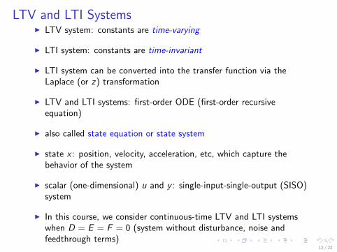
LTV and LTI SystemsI LTV system: constants are time-varying
I LTI system: constants are time-invariant
I LTI system can be converted into the transfer function via theLaplace (or z) transformation
I LTV and LTI systems: first-order ODE (first-order recursiveequation)
I also called state equation or state system
I state x : position, velocity, acceleration, etc, which capture thebehavior of the system
I scalar (one-dimensional) u and y : single-input-single-output (SISO)system
I In this course, we consider continuous-time LTV and LTI systemswhen D = E = F = 0 (system without disturbance, noise andfeedthrough terms)
12 / 22

Discrete-Time LTV and LTI Systems
I discrete-time LTV system
x(t + 1) = A(t)x(t) + B(t)u(t) + D(t)d(t)
y(t) = C (t)x(t) + E (t)u(t) + F (t)n(t)
I discrete-Time LTI System
x(t + 1) = Ax(t) + Bu(t) + Dd(t)
y(t) = Cx(t) + Eu(t) + Fn(t)
I t ∈ Z+ = {0, 1, 2, ...}
I difference equation (first-order recursive equation)
I x , y , u are sequences
I sampled system: x(t) := x(tT ) (T : sampling period)
13 / 22

Nonlinear Systems
I continuous-time nonlinear system
x(t) = f (t, x(t), u(t), d(t)), y(t) = g(t, x(t), u(t), n(t))
I discrete-time nonlinear system
x(t + 1) = f (t, x(t), u(t), d(t)), y(t) = g(t, x(t), u(t), n(t))
I Example: x(t) = x2(t), x(t) = cos(t)
I Linear system can be obtained by linearization of a nonlinear system⇒ next class
14 / 22

Why Study Linear Systems?
I Linear system is a special case of nonlinear systems
I Why do we study linear systems?
I If you do not understand linear systems, you cannot understandnonlinear systems
I Nonlinear systemI Existence of solution?I Hard to analyze its dynamic behaviorI Hard to see its input/output characteristics
I Linear systemI Solution always existsI System characteristics depend on coefficients of the systemI Computationally inexpensiveI Easy to implement (real-time systems)I Linear algebra is the most effective toolI Many applications can be represented by linear systems (circuits,
aircraft, missile, communication, traffic, guidance, economics)
15 / 22

Continuous-Time LTI System
I continuous-time SISO-LTI system
x(t) = Ax(t), x(0) = x0, (A ∈ R, A 6= 0)
I This is a continuous-time SISO autonomous system (no input, u)
I Solution
x(t) = eAtx0
I The behavior of x(t) is determined by the value of A
I A > 0: |x(t)| → ∞ as t →∞ for all x0 ∈ R (unstable)
I A < 0: |x(t)| → 0 as t →∞ for all x0 ∈ R (stable)
I The scalar A determines the speed of convergence or divergence of|x(t)| ( ⇒ system characteristics depend on coefficients of thesystem)
I What if A is a matrix?
16 / 22
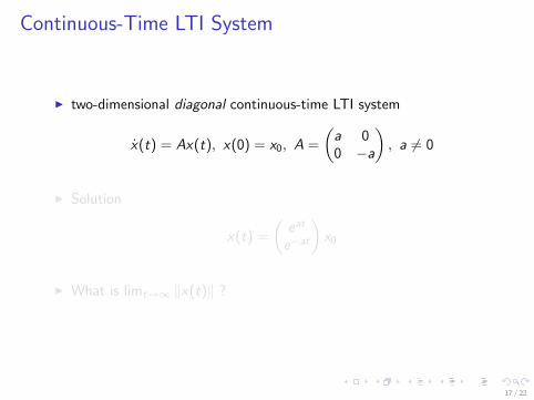
Continuous-Time LTI System
I two-dimensional diagonal continuous-time LTI system
x(t) = Ax(t), x(0) = x0, A =
(a 00 −a
), a 6= 0
I Solution
x(t) =
(eat
e−at
)x0
I What is limt→∞ ‖x(t)‖ ?
17 / 22
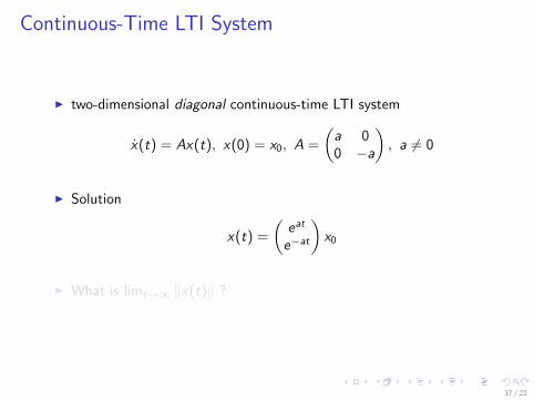
Continuous-Time LTI System
I two-dimensional diagonal continuous-time LTI system
x(t) = Ax(t), x(0) = x0, A =
(a 00 −a
), a 6= 0
I Solution
x(t) =
(eat
e−at
)x0
I What is limt→∞ ‖x(t)‖ ?
17 / 22

Continuous-Time LTI System
I two-dimensional diagonal continuous-time LTI system
x(t) = Ax(t), x(0) = x0, A =
(a 00 −a
), a 6= 0
I Solution
x(t) =
(eat
e−at
)x0
I What is limt→∞ ‖x(t)‖ ?
17 / 22

Continuous-Time LTI System
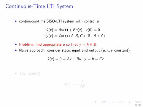
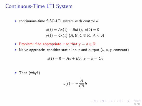
I continuous-time SISO-LTI system with control u
x(t) = Ax(t) + Bu(t), x(0) = 0
y(t) = Cx(t) (A,B,C ∈ R, A < 0)
I Problem: find appropriate u so that y = h ∈ RI Naive approach: consider static input and output (u, x , y constant)
x(t) = 0 = Ax + Bu, y = h = Cx
I Then (why?)
u(t) = − A
CBh
18 / 22
Continuous-Time LTI System
I continuous-time SISO-LTI system with control u
x(t) = Ax(t) + Bu(t), x(0) = 0
y(t) = Cx(t) (A,B,C ∈ R, A < 0)
I Problem: find appropriate u so that y = h ∈ RI Naive approach: consider static input and output (u, x , y constant)
x(t) = 0 = Ax + Bu, y = h = Cx
I Then (why?)
u(t) = − A
CBh
18 / 22

Continuous-Time LTI System
I time-response plot when A = −1, B = C = 1, h = 0.5
I MATLAB Simulink: control system toolbox
19 / 22

Continuous-Time LTI System
I time-response plot when A = −1, B = C = 1, h = 0.5
I MATLAB Simulink: control system toolbox
20 / 22
Continuous-Time LTI System
I This is one simple approach to design u
I There are may ways of designing control u to achieve the desiredcontrol performance
I In this course, we will study some design techniques of u for LTIsystems
I We will not cover classical control theory
21 / 22

Next Class
I classical and modern control theory
I LTI systems
I linearization
I modeling
22 / 22