linear programming simplex algorithm, duality and...
TRANSCRIPT

Linear programming – simplex algorithm, duality anddual simplex algorithm
Martin Branda
Charles University in PragueFaculty of Mathematics and Physics
Department of Probability and Mathematical Statistics
Computational Aspects of Optimization
1 / 32

Linear programming
Content
1 Linear programming
2 Primal simplex algorithm
3 Duality in linear programming
4 Dual simplex algorithm
5 Software tools for LP
2 / 32
Linear programming
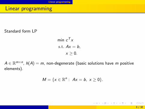
Linear programming
Standard form LP
min cT x
s.t. Ax = b,
x ≥ 0.
A ∈ Rm×n, h(A) = m, non-degenerate (basic solutions have m positiveelements).
M = {x ∈ Rn : Ax = b, x ≥ 0}.
3 / 32
Linear programming
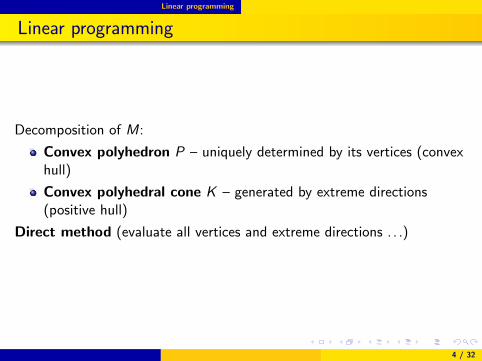
Linear programming
Decomposition of M:
Convex polyhedron P – uniquely determined by its vertices (convexhull)
Convex polyhedral cone K – generated by extreme directions(positive hull)
Direct method (evaluate all vertices and extreme directions . . .)
4 / 32
Linear programming
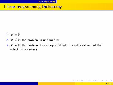
Linear programming trichotomy
1. M = ∅2. M 6= ∅: the problem is unbounded
3. M 6= ∅: the problem has an optimal solution (at least one of thesolutions is vertex)
5 / 32
Primal simplex algorithm
Content
1 Linear programming
2 Primal simplex algorithm
3 Duality in linear programming
4 Dual simplex algorithm
5 Software tools for LP
6 / 32
Primal simplex algorithm
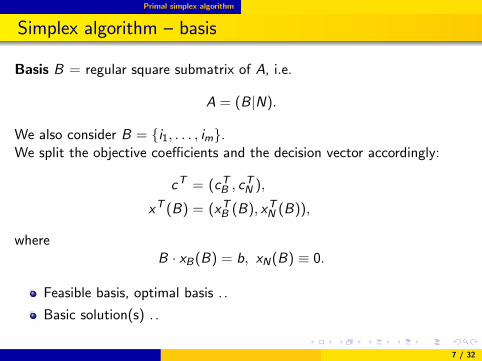
Simplex algorithm – basis
Basis B = regular square submatrix of A, i.e.
A = (B|N).
We also consider B = {i1, . . . , im}.We split the objective coefficients and the decision vector accordingly:
cT = (cTB , cTN ),
xT (B) = (xTB (B), xTN (B)),
whereB · xB(B) = b, xN(B) ≡ 0.
Feasible basis, optimal basis . .
Basic solution(s) . .
7 / 32
Primal simplex algorithm
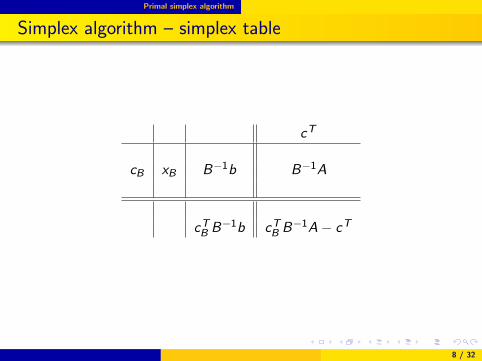
Simplex algorithm – simplex table
cT
cB xB B−1b B−1A
cTB B−1b cTB B
−1A− cT
8 / 32
Primal simplex algorithm
Simplex algorithm – simplex table
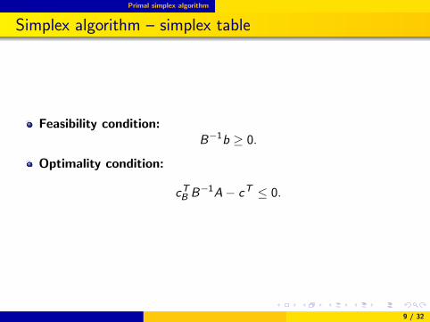
Feasibility condition:B−1b ≥ 0.
Optimality condition:
cTB B−1A− cT ≤ 0.
9 / 32
Primal simplex algorithm
Simplex algorithm – a step
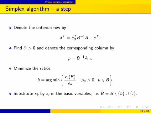
Denote the criterion row by
δT = cTB B−1A− cT .
Find δi > 0 and denote the corresponding column by
ρ = B−1A·,i .
Minimize the ratios
u = arg min{xu(B)
ρu: ρu > 0, u ∈ B
}.
Substitute xu by xi in the basic variables, i.e. B = B \ {u} ∪ {i}.
10 / 32
Primal simplex algorithm
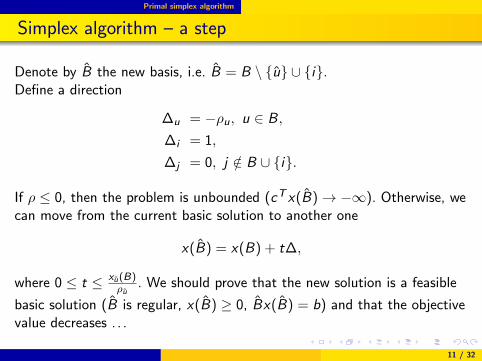
Simplex algorithm – a step
Denote by B the new basis, i.e. B = B \ {u} ∪ {i}.Define a direction
∆u = −ρu, u ∈ B,∆i = 1,
∆j = 0, j /∈ B ∪ {i}.
If ρ ≤ 0, then the problem is unbounded (cT x(B)→ −∞). Otherwise, wecan move from the current basic solution to another one
x(B) = x(B) + t∆,
where 0 ≤ t ≤ xu(B)ρu
. We should prove that the new solution is a feasible
basic solution (B is regular, x(B) ≥ 0, Bx(B) = b) and that the objectivevalue decreases . . .
11 / 32
Primal simplex algorithm
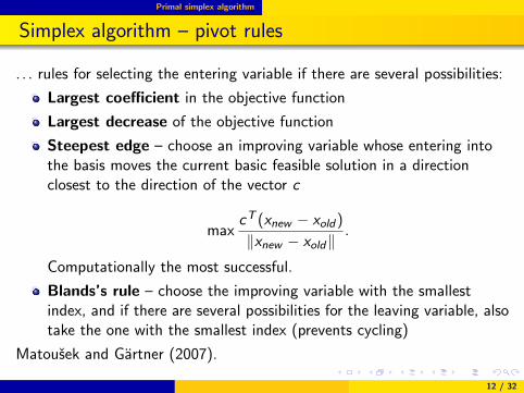
Simplex algorithm – pivot rules
. . . rules for selecting the entering variable if there are several possibilities:
Largest coefficient in the objective function
Largest decrease of the objective function
Steepest edge – choose an improving variable whose entering intothe basis moves the current basic feasible solution in a directionclosest to the direction of the vector c
maxcT (xnew − xold)
‖xnew − xold‖.
Computationally the most successful.
Blands’s rule – choose the improving variable with the smallestindex, and if there are several possibilities for the leaving variable, alsotake the one with the smallest index (prevents cycling)
Matoušek and Gärtner (2007).
12 / 32

Duality in linear programming
Content
1 Linear programming
2 Primal simplex algorithm
3 Duality in linear programming
4 Dual simplex algorithm
5 Software tools for LP
13 / 32
Duality in linear programming
Transportation problem
xij – decision variable: amount transported from i to j
cij – costs for transported unit
ai – capacity
bj – demand
ASS.∑ni=1 ai ≥
∑mj=1 bj .
(Sometimes ai , bj ∈ N.)
14 / 32
Duality in linear programming
Transportation problem
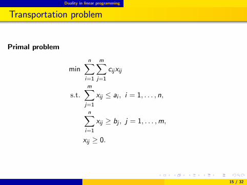
Primal problem
minn∑i=1
m∑j=1
cijxij
s.t.m∑j=1
xij ≤ ai , i = 1, . . . , n,
n∑i=1
xij ≥ bj , j = 1, . . . ,m,
xij ≥ 0.
15 / 32
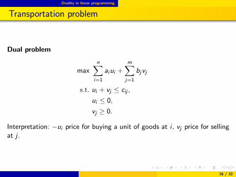
Duality in linear programming
Transportation problem
Dual problem
maxn∑i=1
aiui +m∑j=1
bjvj
s.t. ui + vj ≤ cij ,ui ≤ 0,
vj ≥ 0.
Interpretation: −ui price for buying a unit of goods at i , vj price for sellingat j .
16 / 32
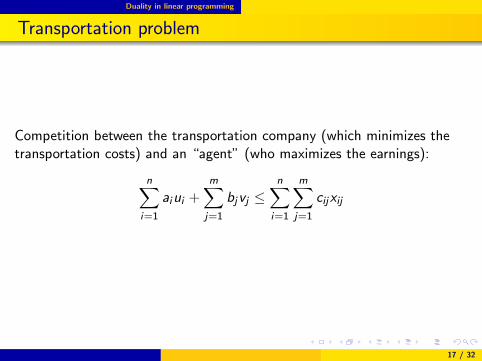
Duality in linear programming
Transportation problem
Competition between the transportation company (which minimizes thetransportation costs) and an “agent” (who maximizes the earnings):
n∑i=1
aiui +m∑j=1
bjvj ≤n∑i=1
m∑j=1
cijxij
17 / 32
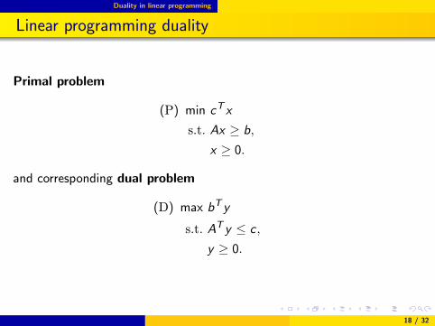
Duality in linear programming
Linear programming duality
Primal problem
(P) min cT x
s.t. Ax ≥ b,x ≥ 0.
and corresponding dual problem
(D) max bT y
s.t. AT y ≤ c ,y ≥ 0.
18 / 32
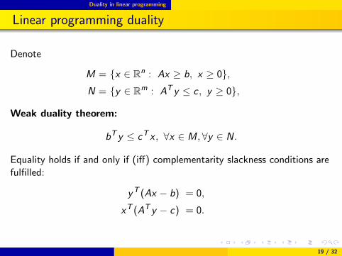
Duality in linear programming
Linear programming duality
Denote
M = {x ∈ Rn : Ax ≥ b, x ≥ 0},N = {y ∈ Rm : AT y ≤ c , y ≥ 0},
Weak duality theorem:
bT y ≤ cT x , ∀x ∈ M, ∀y ∈ N.
Equality holds if and only if (iff) complementarity slackness conditions arefulfilled:
yT (Ax − b) = 0,
xT (AT y − c) = 0.
19 / 32

Duality in linear programming
Linear programming duality
Apply KKT optimality conditions to primal LP . . .
20 / 32
Duality in linear programming
Linear programming duality
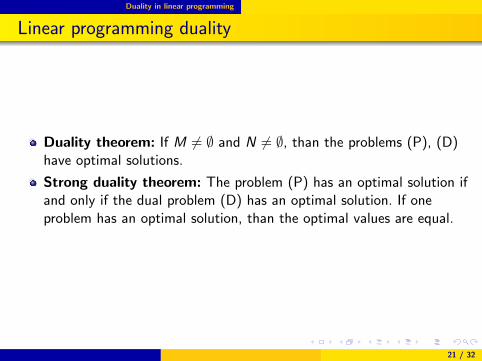
Duality theorem: If M 6= ∅ and N 6= ∅, than the problems (P), (D)have optimal solutions.
Strong duality theorem: The problem (P) has an optimal solution ifand only if the dual problem (D) has an optimal solution. If oneproblem has an optimal solution, than the optimal values are equal.
21 / 32
Dual simplex algorithm
Content
1 Linear programming
2 Primal simplex algorithm
3 Duality in linear programming
4 Dual simplex algorithm
5 Software tools for LP
22 / 32
Dual simplex algorithm
Linear programming duality
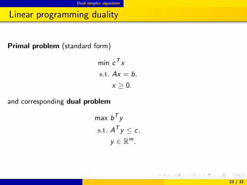
Primal problem (standard form)
min cT x
s.t. Ax = b,
x ≥ 0.
and corresponding dual problem
max bT y
s.t. AT y ≤ c ,y ∈ Rm.
23 / 32
Dual simplex algorithm
Dual simplex algorithm
Basic dual solution
Dual basis
24 / 32
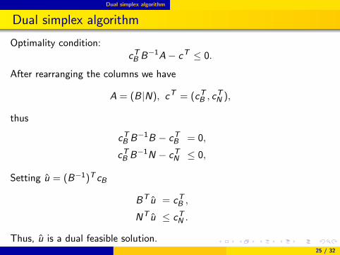
Dual simplex algorithm
Dual simplex algorithm
Optimality condition:cTB B
−1A− cT ≤ 0.
After rearranging the columns we have
A = (B|N), cT = (cTB , cTN ),
thus
cTB B−1B − cTB = 0,
cTB B−1N − cTN ≤ 0,
Setting u = (B−1)T cB
BT u = cTB ,
NT u ≤ cTN .
Thus, u is a dual feasible solution.25 / 32
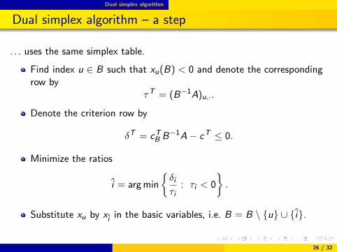
Dual simplex algorithm
Dual simplex algorithm – a step
. . . uses the same simplex table.
Find index u ∈ B such that xu(B) < 0 and denote the correspondingrow by
τT = (B−1A)u,·.
Denote the criterion row by
δT = cTB B−1A− cT ≤ 0.
Minimize the ratios
i = arg min{δiτi
: τi < 0}.
Substitute xu by xi in the basic variables, i.e. B = B \ {u} ∪ {i}.
26 / 32
Dual simplex algorithm
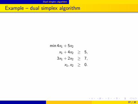
Example – dual simplex algorithm
min 4x1 + 5x2x1 + 4x2 ≥ 5,
3x1 + 2x2 ≥ 7,
x1, x2 ≥ 0.
27 / 32
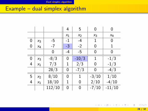
Dual simplex algorithm
Example – dual simplex algorithm
4 5 0 0x1 x2 x3 x4
0 x3 -5 -1 -4 1 00 x4 -7 -3 -2 0 1
0 -4 -5 0 00 x3 -8/3 0 -10/3 1 -1/34 x1 7/3 1 2/3 0 -1/3
28/3 0 -7/3 0 -4/35 x2 8/10 0 1 -3/10 1/104 x1 18/10 1 0 2/10 -4/10
112/10 0 0 -7/10 -11/10
28 / 32

Software tools for LP
Content
1 Linear programming
2 Primal simplex algorithm
3 Duality in linear programming
4 Dual simplex algorithm
5 Software tools for LP
29 / 32

Software tools for LP
Software tools for LP
Matlab
Mathematica
GAMS
MS Excel
. . .
30 / 32
Software tools for LP
Literature
Bazaraa, M.S., Sherali, H.D., and Shetty, C.M. (2006). Nonlinear programming:theory and algorithms, Wiley, Singapore, 3rd edition.
Boyd, S., Vandenberghe, L. (2004). Convex Optimization, Cambridge UniversityPress, Cambridge.
P. Lachout (2011). Matematické programování. Skripta k (zaniklé) přednášceOptimalizace I (IN CZECH).
Matoušek and Gärtner (2007). Understanding and using linear programming,Springer.
31 / 32

Software tools for LP
Questions?
e-mail: [email protected]: http://artax.karlin.mff.cuni.cz/˜ branm1am
32 / 32