linear programming lecture notes for math 3731 introduction to linear programming 1.1 operations...
TRANSCRIPT
Linear ProgrammingLecture Notes for Math 373
Feras Awad
June 21, 2019
Contents
1 Introduction to Linear Programming 31.1 Operations Researches . . . . . . . . . . . . . . . . . . . . . . . 31.2 What is a Linear Programming (LP) Problem? . . . . . . . . . . 31.3 Modeling LP Problems . . . . . . . . . . . . . . . . . . . . . . 51.4 Geometric Preliminaries and Solutions . . . . . . . . . . . . . . 9
1.4.1 Half−Spaces, Hyperplanes, and Convex Sets . . . . . . . 91.4.2 The Graphical Solution of Two−Variable LP Problems . 14
1.5 The Corner Point Theorem and its Proof . . . . . . . . . . . . . 25
2 The Simplex Method 302.1 The Idea of the Simplex Method . . . . . . . . . . . . . . . . . 302.2 Converting an LP to Standard Form . . . . . . . . . . . . . . . 312.3 Basic Feasible Solutions . . . . . . . . . . . . . . . . . . . . . . 322.4 The Simplex Algorithm . . . . . . . . . . . . . . . . . . . . . . 37
2.4.1 Iterative Nature of the Simplex Method . . . . . . . . . 382.4.2 Computational Details of the Simplex Algorithm . . . . . 382.4.3 Representing the Simplex Tableau . . . . . . . . . . . . 39
2.5 Solving Minimization Problem . . . . . . . . . . . . . . . . . . 432.6 Artificial Starting Solution and the Big M−Method . . . . . . . 452.7 Special Cases in the Simplex Method . . . . . . . . . . . . . . . 50
2.7.1 Degeneracy . . . . . . . . . . . . . . . . . . . . . . . . 502.7.2 Alternative Optima . . . . . . . . . . . . . . . . . . . . 572.7.3 Unbounded Solutions . . . . . . . . . . . . . . . . . . . 592.7.4 Nonexisting (or Infeasible) Solutions . . . . . . . . . . . 59
3 Sensitivity Analysis and Duality 653.1 Some Important Formulas . . . . . . . . . . . . . . . . . . . . . 653.2 Sensitivity Analysis . . . . . . . . . . . . . . . . . . . . . . . . 703.3 Finding the Dual of an LP . . . . . . . . . . . . . . . . . . . . 753.4 The Dual Theorem and its Consequences . . . . . . . . . . . . 77
1

3.5 Shadow Prices . . . . . . . . . . . . . . . . . . . . . . . . . . . 843.6 Duality and Sensitivity Analysis . . . . . . . . . . . . . . . . . . 863.7 Complementary Slackness . . . . . . . . . . . . . . . . . . . . . 893.8 The Dual−Simplex Method . . . . . . . . . . . . . . . . . . . . 92
Answers 100
2
1 Introduction to Linear Programming
1.1 Operations Researches
The first formal activity of operations research (OR) were initiated in Englandduring World War II. A team of British scientists set out to make decisionsregarding the best utilization of war materials. After war, the idea was adoptedand improved in the civilian sector.
In OR, we do not have a single general technique to solve all mathematicalmodels. The most OR techniques are: Linear Programming, Non-Linear Pro-gramming, Integer Programming, Dynamic Programming, Network Program-ming, and much more. All techniques are determined by algorithms, and notby closed form formulas. The algorithms are for deterministic models (not forprobability or stochastic model). Deterministic means when we know the valuesof the variables we know the value of the model in certainty.
1.2 What is a Linear Programming (LP) Problem?
Definition 1.1. A function f (x1, x2, · · · , xn) of the vari-ables x1, x2, · · · , xn is a linear function if f (x1, x2, · · · , xn) =c1x1 + c2x2 + · · ·+ cnxn where c1, c2, · · · , cn are constants.
Example 1.1. f (x1, x2) = 2x1 + x2 is linear function, while f (x1, x2) = x21x2is not linear.
Definition 1.2. For any linear function f (x1, x2, · · · , xn) andany real number b, the inequalities f (x1, x2, · · · , xn) ≤ b andf (x1, x2, · · · , xn) ≥ b are linear inequalities.
Example 1.2. 2x1 + 3x2 ≤ 3 is linear inequality, while x1x2 +√x2 ≥ 3 is not
linear inequality.
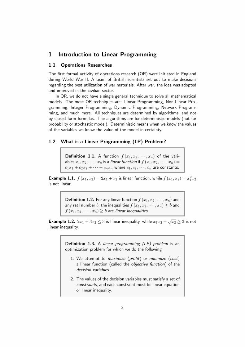
Definition 1.3. A linear programming (LP) problem is anoptimization problem for which we do the following
1. We attempt to maximize (profit) or minimize (cost)a linear function (called the objective function) of thedecision variables.
2. The values of the decision variables must satisfy a set ofconstraints, and each constraint must be linear equationor linear inequality.
3

3. A sign restriction is associated with each variable. Forany variable xi, either xi ≥ 0 or xi is unrestricted insign (urs).
max (or min) z = f (x1, x2, · · · , xn)Subject to Constraints
Sign Restriction.
Example 1.3. Furnco manufactures desks and chairs. Each desk uses 4 unitsof wood, and each chair uses 3. A desk contributes $40 to profit, and a chaircontributes $25. Marketing restrictions require that the number of chairs pro-duced be at least twice the number of desks produced. If 20 units of wood areavailable, formulate an LP to maximize Furnco’s profit.
Solution: Let x1 be the number of desks produced, and x2 be the numberof chairs produced. Then, the formulation of the problem is
max z = 40x1 + 25x2s.t. 4x1 + 3x2 ≤ 20
x2 ≥ 2x1x1 ≥ 0, x2 ≥ 0
The optimal solution of this problem is x1 = 2, x2 = 4, and z = 180. (We willsee how we find these values later on.)
Note 1. [LP Assumptions]
1. The Proportionality and Additivity Assumptions.The fact that the objective function for an LP must be a linear functionof the decision variables has two implications.
(a) The contribution of the objective function from each decision vari-able is proportional to the value of the decision variable. For exam-ple, the contribution to the objective function in example (1.3) frommaking 5 desks is exactly five times the contribution to the objectivefunction from making one desk.
(b) The contribution to the objective function for any variable is inde-pendent of the values of the other decision variables. For example,no matter what the value of x2, the manufacture of x1 desks willalways contribute 40x1 dollars to the objective function.
Analogously, the fact that each LP constraint must be a linear inequalityor linear equation has two implications.
(a) The contribution of each variable to the lefthand side of each con-straint is proportional to the value of the variable.
(b) The contribution of a variable to the lefthand side of each constraintis independent of the values of the variable.
4

2. The Divisibility Assumption.The divisibility assumption requires that each decision variable be allowedto assume fractional values. For instance, in example (1.3), the DivisibilityAssumption implies that it is acceptable to produce 1.5 desks or 1.63chairs. Because Frunco cannot actually produce a fractional number ofdesks or chairs, the Divisibility Assumption is not satisfied in the Fruncoproblem. A linear programming problem in which some or all of thevariables must be nonnegative integers is called an integer programmingproblem.
3. The Certainty Assumption.The certainty assumption is that each parameter (objective function coef-ficient, righthand side, and constraint coefficient) is known with certainty.If we were unsure of the exact amount of wood used by desks and chairs,the Certainty Assumption would be violated.
1.3 Modeling LP Problems
This section presents LP models in which the definition of the variables and theconstruction of the objective function and constraints are not straightforward.
Example 1.4. Giapetto’s Woodcarving, Inc., manufactures two types of woodentoys: soldiers and trains. A soldier sells for $27 and uses $10 worth of rawmaterials. Each soldier that is manufactured increases Giapetto’s variable laborand overhead costs by $14. A train sells for $21 and uses $9 worth of rawmaterials. Each train built increases Giapetto’s variable labor and overheadcosts by $10. The manufacture of wooden soldiers and trains requires two typesof skilled labor: carpentry and finishing. A soldier requires 2 hours of finishinglabor and 1 hour of carpentry labor. A train requires 1 hour of finishing and1 hour of carpentry labor. Each week, Giapetto can obtain all the needed rawmaterial but only 100 finishing hours and 80 carpentry hours. Demand for trainsis unlimited, but at most 40 soldiers are bought each week. Giapetto wants tomaximize weekly profit (revenues - costs). Formulate a mathematical model ofGiapetto’s situation that can be used to maximize Giapetto’s weekly profit.
Solution: Let x1 = number of soldiers produced each week, x2 = numberof trains produced each week. Then, the formulation of the problem is
max z = 3x1 + 2x2s.t. 2x1 + x2 ≤ 100
x1 + x2 ≤ 80x1 ≤ 40x1 ≥ 0, x2 ≥ 0
Example 1.5. Farmer Jones must determine how many acres of corn and wheatto plant this year. An acre of wheat yields 25 bushels of wheat and requires 10hours of labor per week. An acre of corn yields 10 bushels of corn and requires
5

4 hours of labor per week. All wheat can be sold at $4 a bushel, and all corncan be sold at $3 a bushel. Seven acres of land and 40 hours per week of laborare available. Government regulations require that at least 30 bushels of cornbe produced during the current year. formulate an LP whose solution will tellFarmer Jones how to maximize the total revenue from wheat and corn.
Solution: We can formulate this problem in two ways, depending on yourassumption for the decision variables.
Method [1] : Method [2] :
x1 = number of acres of wheatplanted.
x1 = number of bushels ofwheat produced.
x2 = number of acres of cornplanted.
x2 = number of bushels of cornproduced.
max z = 100x1 + 30x2s.t. x1 + x2 ≤ 7
10x2 ≥ 3010x1 + 4x2 ≤ 40x1 ≥ 0, x2 ≥ 0
max z = 4x1 + 3x2
s.t.1
25x1 +
1
10x2 ≤ 7
x2 ≥ 3010
25x1 +
4
10x2 ≤ 40
x1 ≥ 0, x2 ≥ 0
Example 1.6. The Village Butcher Shop traditionally makes its meat loaf froma combination of lean ground beef and ground pork. The ground beef contains80 percent meat and 20 percent fat, and costs the shop $80 ; per pound; theground pork contains 68 percent meat and 32 percent fat, and costs $60 ; perpound. Formulate an LP to minimize Village Butcher Shop’s cost of each kindof meat should the shop use in each pound of meat loaf and to keep the fatcontent of the meat loaf to no more than 25 percent?
Solution: Let x1 = poundage of ground beef used in each pound of meatloaf, x2 = poundage of ground pork used in each pound of meat loaf. Then,the formulation of the problem is
min w = 80x1 + 60x2s.t. 0.20x1 + 0.32x2 ≤ 0.25
x1 + x2 = 1x1 ≥ 0, x2 ≥ 0
Example 1.7. Steelco manufactures two types of steel at three different steelmills. During a given month, each steel mill has 200 hours of blast furnace timeavailable. Because of differences in the furnaces at each mill, the time and costto produce a ton of steel differs for each mill. The time and cost for each millare shown in the table. Each month, Steelco must manufacture at least 500tons of steel 1 and 600 tons of steel 2. Formulate an LP to minimize the costof manufacturing the desired steel.
6

Steel 1 Steel 1Mill Cost Time Cost Time
(Minutes) (Minutes)1 $10 20 $11 222 $12 24 $09 183 $14 28 $10 30
Solution: Let xij = number of tons of Steel j produced each month at Milli. Then a correct formulation is
min w = 10x11 + 12x21 + 14x31 + 11x12 + 9x22 + 10x32s.t. 20x11+ 22x12 ≤ 12000
24x21+ 18x22 ≤ 1200028x31+ 30x32 ≤ 12000
x11+ x21+ x31+ ≥ 500x12+ x22+ x32 ≥ 600
x11, x12, x13, x21, x22, x23 ≥ 0
Exercise 1.1.
1. A furniture company manufactures desks and chairs. The sawing depart-ment cuts the lumber for both products, which is then sent to separateassembly departments. Assembled items are sent for finishing to the paint-ing department. The daily capacity of the sawing department is 200 chairsor 80 desks. The chair assembly department can produce 120 chairs dailyand the desk assembly department 60 desks daily. The paint departmenthas a daily capacity of either 150 chairs or 110 desks. Given that theprofit per chair is $50 and that of a desk is $100, formulate an LP tomaximize the company’s profit.
2. Truckco manufactures two types of trucks: 1 and 2. Each truck must gothrough the painting shop and assembly shop. If the painting shop werecompletely devoted to painting Type 1 trucks, then 800 per day could bepainted; if the painting shop were completely devoted to painting Type2 trucks, then 700 per day could be painted. If the assembly shop werecompletely devoted to assembling truck 1 engines, then 1,500 per daycould be assembled; if the assembly shop were completely devoted toassembling truck 2 engines, then 1,200 per day could be assembled. EachType 1 truck contributes $300 to profit; each Type 2 truck contributes$500. Formulate an LP to maximize Truckco’s profit.
3. Assume you want to decide between alternate ways of spending an eight-hour day, that is, you want to allocate your resource time. Assume youfind it five times more fun to play ping-pong in the lounge than to work,but you also feel that you should work at least three times as many hoursas you play ping-pong. Now the decision problem is how many hours to
7

play and how many to work in order to maximize your fun. Formulatethis problem.
4. Leary Chemical manufactures three chemicals: A, B, and C. These chemi-cals are produced via two production processes: 1 and 2. Running process1 for an hour costs $4 and yields 3 units of A, 1 of B, and 1 of C. Runningprocess 2 for an hour costs $1 and produces 1 unit of A and 1 of B. Tomeet customer demands, at least 10 units of A, 5 of B, and 3 of C mustbe produced daily. Formulate an LP to minimize Leary Chemical’s costof daily demands.
5. A company produces two products, A and B. The sales volume for A isat least 80% of the total sales of both A and B. However, the companycannot sell more than 100 units of A per day. Both products use one rawmaterial, of which the maximum daily availability is 240 lb. The usagerates of the raw material are 2 lb per unit of A and 4 lb per unit of B.The profit units for A and B are $20 and $50, respectively. Formulate anLP to maximize the company’s profit.
6. A banquet hall offers two types of tables for rent: 6−person rectangulartables at a cost of $28 each and 10−person round tables at a cost of $52each. Kathleen would like to rent the hall for a wedding banquet andneeds tables for 250 people. The room can have a maximum of 35 tablesand the hall only has 15 rectangular tables available. Formulate an LP tominimize the cost of each type of tables should be rented.
7. A diet is to contain at least 400 units of vitamins, 500 units of minerals,and 1400 calories. Two foods are available: F1, which costs $0.05 perunit, and F2, which costs $0.03 per unit. A unit of food F1 contains 2units of vitamins, 1 unit of minerals, and 4 calories; a unit of food F2contains 1 unit of vitamins, 2 units of minerals, and 4 calories. Formulatean LP to minimize the cost for a diet that consists of a mixture of thesetwo foods and also meets the minimal nutrition requirements.
8. An appliance company has a warehouse and two terminals. To minimizeshipping costs, the manager must decide how many appliances should beshipped to each terminal. There is a total supply of 1200 units in thewarehouse and a demand for 400 units in terminal A and 500 units interminal B. It costs $12 to ship each unit to terminal A and $16 to shipto terminal B. Formulate an LP to minimize the cost of units shipping toeach terminal.
9. Katy needs at least 60 units of carbohydrates, 45 units of protein, and 30units of fat each month. From each pound of food A, she receives 5 unitsof carbohydrates, 3 of protein, and 4 of fat. Food B contains 2 units ofcarbohydrates, 2 units of protein, and 1 unit of fat per pound. If food A
8

costs $1.30 per pound and food B costs $0.80 per pound, formulate anLP to minimize the cost of pounds of each food should Katy buy eachmonth.
1.4 Geometric Preliminaries and Solutions
Any LP with only two variables can be solved graphically. We always label thevariables x1 and x2 and the coordinate axes the x1 and x2 axes.
1.4.1 Half−Spaces, Hyperplanes, and Convex Sets
Definition 1.4. We define the Euclidean plane Rn to be theset of all n−tuples of real numbers; that is
Rn ={
(x1, x2, · · · , xn)∣∣ xi ∈ R for i = 1, 2, · · · , n
}For example, R2 =
{(x1, x2)
∣∣ x1 and x2 are reals}
. Geometrically, werepresent R2 as in Figure 1.
Figure 1
The graph in R2 of an equation of the form a1x1+a2x2 = c (where a1, a2, care constants) is a straight line. For example, the graph in R2 of the equation2x1 − 3x2 = 6 is the line indicated in Figure 2.
Figure 2
9

The graph in R2 of the inequality a1x1 + a2x2 ≤ c or a1x1 + a2x2 ≥ c isthe set of all points in R2 lying on the line a1x1 + a2x2 = c together with allpoints lying to one side of this line. For example, the shaded region in Figure3 is the graph of the inequality 2x1 − 3x2 ≤ 6. To determine on which side of
Figure 3
the line where the region of the inequality 2x1 − 3x2 ≤ 6 lies, consider a point,say (0, 0), not lying on the line but satisfying the inequality; the side of the linecontaining this point is the one corresponding to the inequality.
Definition 1.5. A half−space in Rn is the set of all points inRn satisfying an inequality of the form
a1x1 + a2x2 + · · ·+ anxn ≤ c
or an inequality of the form
a1x1 + a2x2 + · · ·+ anxn ≥ c
where at least one of the constants a1, a2, · · · , an is nonzero.
Definition 1.6. A hyperplane in Rn is the set of all points inRn satisfying an equality of the form
a1x1 + a2x2 + · · ·+ anxn = c
where at least one of the constants a1, a2, · · · , an is nonzero.
For example, the set of points in R5 satisfying
3x1 +1
2x2 − x3 + x4 +
2
3x5 = −9
10
is a hyperplane in R5, and the set of points in R5 satisfying
3x1 +1
2x2 − x3 + x4 +
2
3x5 ≥ −9
is a half-space in R5.
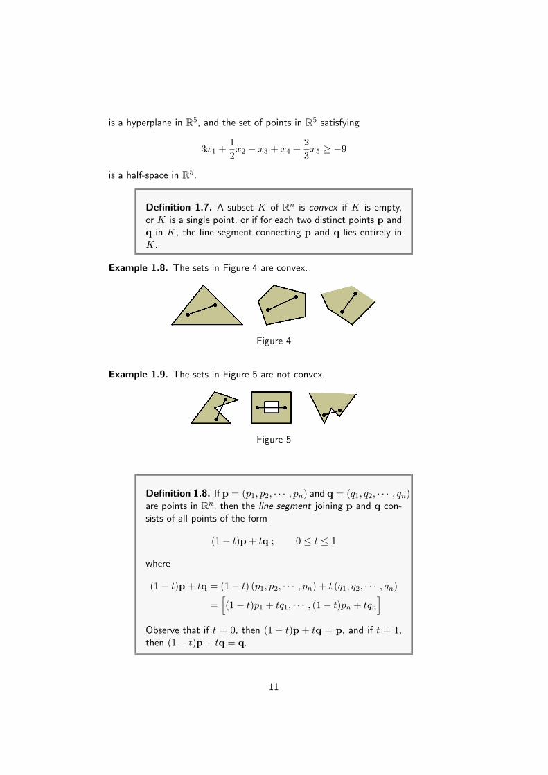
Definition 1.7. A subset K of Rn is convex if K is empty,or K is a single point, or if for each two distinct points p andq in K, the line segment connecting p and q lies entirely inK.
Example 1.8. The sets in Figure 4 are convex.
Figure 4
Example 1.9. The sets in Figure 5 are not convex.
Figure 5
Definition 1.8. If p = (p1, p2, · · · , pn) and q = (q1, q2, · · · , qn)are points in Rn, then the line segment joining p and q con-sists of all points of the form
(1− t)p + tq ; 0 ≤ t ≤ 1
where
(1− t)p + tq = (1− t) (p1, p2, · · · , pn) + t (q1, q2, · · · , qn)
=[(1− t)p1 + tq1, · · · , (1− t)pn + tqn
]Observe that if t = 0, then (1 − t)p + tq = p, and if t = 1,then (1− t)p + tq = q.
11

Example 1.10. The line segment in R2 joining the points p = (3, 6) andq = (−4, 5) is the set of points
(1− t)p + tq = (1− t) (3, 6) + t (−4, 5)
=[3(1− t)− 4t, 6(1− t) + 5t
]=(3− 7t, 6− t
); 0 ≤ t ≤ 1
Theorem 1.1. A half-space H in Rn that is defined either bythe inequality
a1x1 + a2x2 + · · ·+ anxn ≤ c
or the inequality
a1x1 + a2x2 + · · ·+ anxn ≥ c
is convex.
Proof. We establish this result for the half-space H defined by the inequality
a1x1 + a2x2 + · · ·+ anxn ≤ c (1.1)
A similar argument hold for half-spaces defined by a1x1+a2x2+ · · ·+anxn ≥ c.Suppose the points p = (p1, · · · , pn) and q = (q1, · · · , qn) lie in H; that is,these points satisfy inequality (1.1), so we have
a1p1 + a2p2 + · · ·+ anpn ≤ c
a1q1 + a2q2 + · · ·+ anqn ≤ c
To show that the line segment connecting these two points lies entirely in H,it suffices to show that for each t ∈
[0, 1], the point
(1− t)p + tq =[(1− t)p1 + tq1, · · · , (1− t)pn + tqn
]also satisfies inequality (1.1). To show this, we have
a1 [(1− t)p1 + tq1] + a2 [(1− t)p2 + tq2] + · · ·+ an [(1− t)pn + tqn]
= (1− t) (a1p1 + a2p2 + · · ·+ anpn) + t (a1q1 + a2q2 + · · ·+ anqn)
≤ (1− t)c + tc = c
and this concludes the proof. �
12
Theorem 1.2. If K1,K2, · · · ,Kr are convex subsets of Rn,then the intersection of these sets, K = K1 ∩K2 ∩ · · · ∩Kr
is also convex.
Proof. If K is empty or consists of a single point, then K is convex by definition(1.7). Suppose then that K consists of more than one point, and let p andq be any two distinct points in K. Since p and q are in each convex set Ki;1 ≤ i ≤ r, the line segment L connecting p and q also lies entirely in each Ki.Therefore, L lies in the intersection K of these sets, and we conclude that Kis convex. �
Theorem 1.3. A hyperplane M in Rn defined by
a1x1 + a2x2 + · · ·+ anxn = c
is convex
Proof. M is the intersection of the convex half-spaces
a1x1 + a2x2 + · · ·+ anxn ≤ c
anda1x1 + a2x2 + · · ·+ anxn ≥ c
By Theorem (1.2), this intersection is convex. �
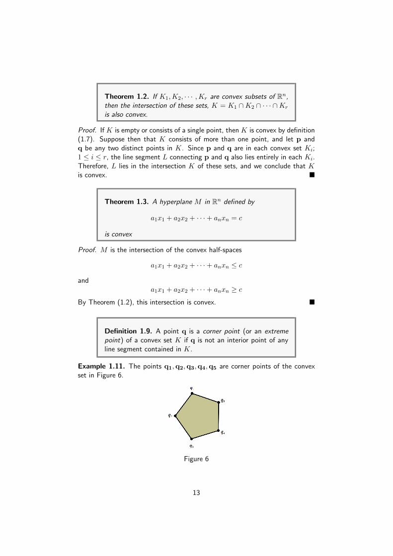
Definition 1.9. A point q is a corner point (or an extremepoint) of a convex set K if q is not an interior point of anyline segment contained in K.
Example 1.11. The points q1,q2,q3,q4,q5 are corner points of the convexset in Figure 6.
Figure 6
13

Exercise 1.2.
1. Draw the graph in R2 of the following half-spaces.
(a) −2x1 + 4x2 ≥ 12.
(b) x2 ≤ 2x1.
(c) x1 ≥ 4.
(d) −3x2 ≤ 9
2. Which of the following expressions define hyperplanes, half-spaces, orneither?
(a) 2x1 + 3x2 = x2 − x4 + 3.
(b) x1 − 3x4 ≥ 3x2 + x3.
(c) x1x2 ≤ 1.
(d) x1 = 6 +2
x2.
(e) 2.5x1 − 3.2x2 = 10.
(f) x1 + x32 ≥ 9.
3. Which of the following sets in Figure 7 are convex?
Figure 7
4. Let p = (1, 3, 2) and q = (2, 4,−1) be two points in R3.
(a) Find the set of points that lie on the line segment joining the pointsp and q.
(b) Show that the point (1.5, 3.5, 0.5) lies on the line segment joiningthe points p and q.
1.4.2 The Graphical Solution of Two−Variable LP Problems
Two of the most basic concepts associated with a linear programming problemare feasible region and optimal solution. For defining these concepts, we usethe term point to mean a specification of the value for each decision variable.
14
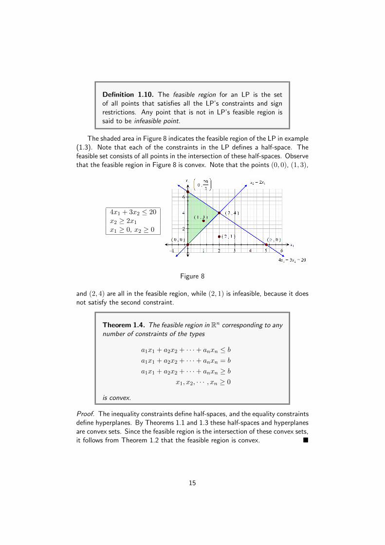
Definition 1.10. The feasible region for an LP is the setof all points that satisfies all the LP’s constraints and signrestrictions. Any point that is not in LP’s feasible region issaid to be infeasible point.
The shaded area in Figure 8 indicates the feasible region of the LP in example(1.3). Note that each of the constraints in the LP defines a half-space. Thefeasible set consists of all points in the intersection of these half-spaces. Observethat the feasible region in Figure 8 is convex. Note that the points (0, 0), (1, 3),
4x1 + 3x2 ≤ 20x2 ≥ 2x1x1 ≥ 0, x2 ≥ 0
Figure 8
and (2, 4) are all in the feasible region, while (2, 1) is infeasible, because it doesnot satisfy the second constraint.
Theorem 1.4. The feasible region in Rn corresponding to anynumber of constraints of the types
a1x1 + a2x2 + · · ·+ anxn ≤ b
a1x1 + a2x2 + · · ·+ anxn = b
a1x1 + a2x2 + · · ·+ anxn ≥ b
x1, x2, · · · , xn ≥ 0
is convex.
Proof. The inequality constraints define half-spaces, and the equality constraintsdefine hyperplanes. By Theorems 1.1 and 1.3 these half-spaces and hyperplanesare convex sets. Since the feasible region is the intersection of these convex sets,it follows from Theorem 1.2 that the feasible region is convex. �
15

Definition 1.11. For a maximization (minimization) problem,an optimal solution to an LP is a point in the feasible regionwith the largest (smallest) objective function value.
The goal of any LP problem is to find the optimum, the best feasible solutionthat maximizes the total profit or minimizes the cost. Having identified thefeasible region for the Furnco problem in example (1.3) as shown in Figure 8,we now search for the optimal solution, which will be the point in the feasibleregion with the largest value of z = 40x1 + 25x2.
� To find the optimal solution, we need to graph a line on which all pointshave the same z−value. In a max problem, such a line is called an isoprofitline.
� To draw an isoprofit line, choose any point in the feasible region andcalculate its z−value. Let us choose (1, 3). For (1, 3), z = 40(1) +25(3) = 115. Thus, (1, 3) lies on the isoprofit line z = 40x1+25x2 = 115.
� Because all isoprofit lines are of the form 40x1 + 25x2 = constant, allisoprofit lines have the same slope. This means that once we have drawnone isoprofit line, we can find all other isoprofit lines by moving parallelto the isoprofit line we have drawn in a direction that increases z.
� After a point, the isoprofit lines will no longer intersect the feasible region.The last isoprofit line intersecting (touching) the feasible region definesthe largest z−value of any point in the feasible region and indicates theoptimal solution to the LP.
� In our problem, the objective function z = 40x1 + 25x2 will increase if wemove in a direction for which both x1 and x2 increase. Thus, we constructadditional isoprofit lines by moving parallel to 40x1 + 25x2 = 115 in anortheast direction (upward and to the right), as shown in Figure 9.
Figure 9
16

� From Figure 9, we see that the isoprofit line passing through point (2, 4)is the last isoprofit line to intersect the feasible region. Thus, (2, 4) is thepoint in the feasible region with the largest z−value and is therefore theoptimal solution to the Furnco problem. Thus, the optimal value of z isz = 40(2) + 25(4) = 180.
Example 1.12. Graphically solve the following LP problem.
max z = 3x1 + 2x2s.t. 2x1 + x2 ≤ 100
x1 + x2 ≤ 80x1 ≤ 40x1 ≥ 0, x2 ≥ 0
Solution: From Figure 10,the isoprofitlines maximizes the value of the objectivefunction by increasing z in the northeastdirection (up-right). The optimum solu-tion is the intersection of the two lines2x1 +x2 = 100 and x1 +x2 = 80, whichyields x1 = 20 and x2 = 60. The maxi-mum value of z is z = 3(20) + 2(60) =180.
Figure 10
Note 2. In a minimization problem, to find the optimal solution, we need tograph a line on which all points have the same w−value, such a line is called anisocost line. Once we have drawn one isocost line, we can find all other isocostlines by moving parallel to the isocost line we have drawn first in a directionthat decreases w. After a point, the isocost lines will no longer intersect thefeasible region. The last isocost line intersecting the feasible region defines thesmallest w−value of any point in the feasible region and indicates the optimalsolution to the LP.
Example 1.13. Graphically solve the following LP problem.
min w = −4x1 + 7x2s.t. x1 + x2 ≥ 3
−x1 + x2 ≤ 32x1 + x2 ≤ 8x1 ≥ 0, x2 ≥ 0
Solution: From Figure 11,The isocost lines minimizes the value of the objectivefunction by decreasing w in the southeast direction (down-right). The optimum
17
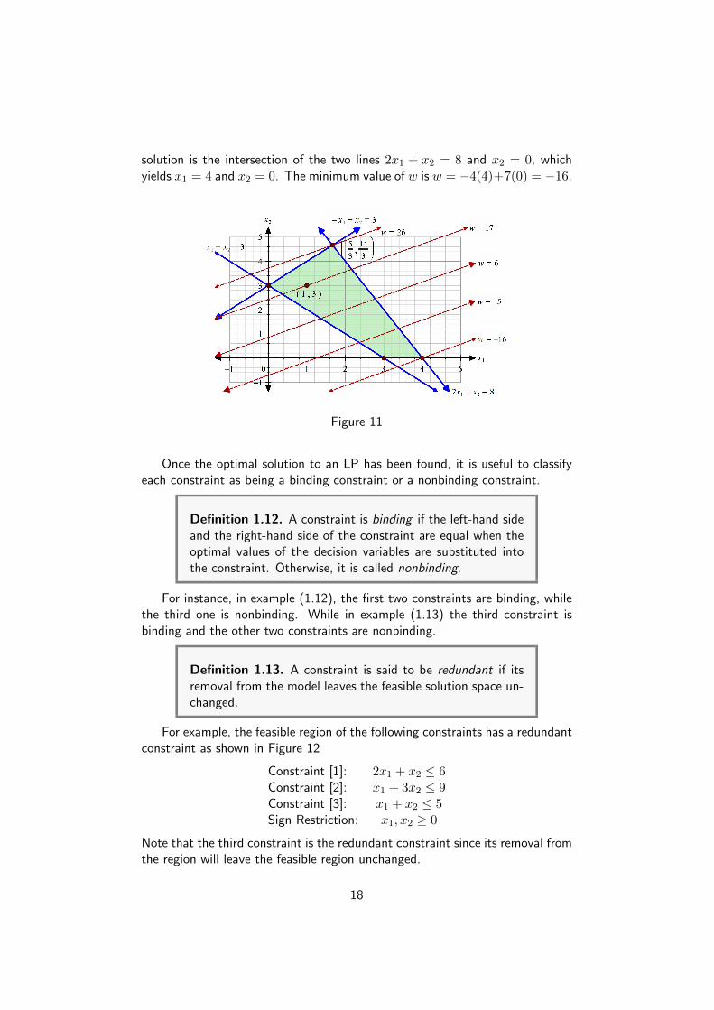
solution is the intersection of the two lines 2x1 + x2 = 8 and x2 = 0, whichyields x1 = 4 and x2 = 0. The minimum value of w is w = −4(4)+7(0) = −16.
Figure 11
Once the optimal solution to an LP has been found, it is useful to classifyeach constraint as being a binding constraint or a nonbinding constraint.
Definition 1.12. A constraint is binding if the left-hand sideand the right-hand side of the constraint are equal when theoptimal values of the decision variables are substituted intothe constraint. Otherwise, it is called nonbinding.
For instance, in example (1.12), the first two constraints are binding, whilethe third one is nonbinding. While in example (1.13) the third constraint isbinding and the other two constraints are nonbinding.
Definition 1.13. A constraint is said to be redundant if itsremoval from the model leaves the feasible solution space un-changed.
For example, the feasible region of the following constraints has a redundantconstraint as shown in Figure 12
Constraint [1]: 2x1 + x2 ≤ 6Constraint [2]: x1 + 3x2 ≤ 9Constraint [3]: x1 + x2 ≤ 5Sign Restriction: x1, x2 ≥ 0
Note that the third constraint is the redundant constraint since its removal fromthe region will leave the feasible region unchanged.
18

Figure 12
Note 3. [Alternative Optima] An LP problem may have an infinite numberof alternative optima when the objective function is parallel to a nonredundantbinding constraint. This is indicated by the fact that as an isoprofit (or isocost)line leaves the feasible region, it will intersect an entire line segment corre-sponding to the binding constraint. It seems reasonable that if two points areoptimal, then any point on the line segment joining these two points will alsobe optimal. If an alternative optimum occurs, then the decision maker can usea secondary criterion to choose between optimal solutions. The technique ofgoal programming is often used to choose among alternative optimal solutions.The next example demonstrates the practical significance of such solutions.
Example 1.14. Graphically solve the following LP problem.
max z = 4x1 + x2s.t. 8x1 + 2x2 ≤ 16
5x1 + 2x2 ≤ 12x1, x2 ≥ 0
Solution: The feasible region for this LP is the shaded region in Figure 13.For our isoprofit line, we choose the line passing through the point (0.4, 1).Because (0.4, 1) has a z−value of 4(0.4) + (1) = 2.6, this yields the isoprofitline z = 4x1 + x2 = 2.6. Examining lines parallel to this isoprofit line in thedirection of increasing z (northeast), we find that the last “point” in the feasibleregion to intersect an isoprofit line is the entire line segment joining the cornerpoints
(43 ,
83
)and (2, 0). This means that any point on this line segment is
optimal. These points are given by
t
(4
3,8
3
)+ (1− t)(2, 0) =
(2− 2t
3,8t
3
); 0 ≤ t ≤ 1
19

Figure 13
Note 4. [Infeasible LP] It is possible for an LP’s feasible region to be empty(contain no points), resulting in an infeasible LP. Because the optimal solutionto an LP is the best point in the feasible region, an infeasible LP has no optimalsolution.
Example 1.15. The following LP problem has no feasible solution as shown inFigure 14.
max z = 3x1 + 2x2s.t. 3x1 + 2x2 ≤ 120
x1 + x2 ≤ 50x1 ≥ 30x2 ≥ 20x1, x2 ≥ 0
Figure 14
Note 5. [Unbounded LP] For a max problem, an unbounded LP occurs if it ispossible to find points in the feasible region with arbitrarily large z−values, whichcorresponds to a decision maker earning arbitrarily large revenues or profits.This would indicate that an unbounded optimal solution should not occur in acorrectly formulated LP. Thus, if the reader ever solves an LP on the computerand finds that the LP is unbounded, then an error has probably been made informulating the LP or in inputting the LP into the computer. For a minimizationproblem, an LP is unbounded if there are points in the feasible region witharbitrarily small z−values. When graphically solving an LP, we can spot anunbounded LP as follows:
� A max problem is unbounded if, when we move parallel to our originalisoprofit line in the direction of increasing z, we never entirely leave thefeasible region.
20

� A minimization problem is unbounded if we never leave the feasible regionwhen moving in the direction of decreasing z.
Example 1.16. Graphically solve the following LP problem.
max z = 2x1 − x2s.t. x1 − x2 ≤ 1
2x1 + x2 ≥ 6x1, x2 ≥ 0
Solution: The feasible region is the(shaded) unbounded region in Figure 15.To find the optimal solution, we draw theisoprofit line passing through (2, 5). Thisisoprofit line has z = 2(2) − (5) = −1.The direction of increasing z is to thesoutheast (this makes x1 larger and x2smaller). Moving parallel to z = 2x1−x2in a southeast direction, we see thatany isoprofit line we draw will intersectthe feasible region. (This is becauseany isoprofit line is steeper than the linex1 − x2 = 1.) Thus, there are points inthe feasible region that have arbitrarilylarge z-values.
Figure 15
Example 1.17. Graphically solve the following LP problem.
min w = 0.3x1 + 0.9x2s.t. x1 + x2 ≥ 800
7x1 − 10x2 ≤ 03x1 − x2 ≥ 0x1, x2 ≥ 0
Figure 16
Solution: Although the feasible region of the LP is unbounded, but it hasoptimal solution as shown in Figure 16.
21
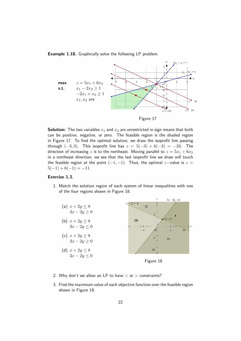
Example 1.18. Graphically solve the following LP problem.
max z = 5x1 + 6x2s.t. x1 − 2x2 ≥ 1
−2x1 + x2 ≥ 1x1, x2 urs
Figure 17
Solution: The two variables x1 and x2 are unrestricted in sign means that bothcan be positive, negative, or zero. The feasible region is the shaded regionin Figure 17. To find the optimal solution, we draw the isoprofit line passingthrough (−3, 3). This isoprofit line has z = 5(−3) + 6(−3) = −33. Thedirection of increasing z is to the northeast. Moving parallel to z = 5x1 + 6x2in a northeast direction, we see that the last isoprofit line we draw will touchthe feasible region at the point (−1,−1). Thus, the optimal z−value is z =5(−1) + 6(−1) = −11.
Exercise 1.3.
1. Match the solution region of each system of linear inequalities with oneof the four regions shown in Figure 18.
(a) x + 2y ≤ 83x− 2y ≥ 0
(b) x + 2y ≥ 83x− 2y ≤ 0
(c) x + 2y ≥ 83x− 2y ≥ 0
(d) x + 2y ≤ 83x− 2y ≤ 0
Figure 18
2. Why don’t we allow an LP to have < or > constraints?
3. Find the maximum value of each objective function over the feasible regionshown in Figure 19.
22

(a) z = x + y
(b) z = 4x + y
(c) z = 3x + 7y
(d) z = 9x + 3y
Figure 19
4. Find the minimum value of each objective function over the feasible regionshown in Figure 20.
(a) w = 7x + 4y
(b) w = 7x + 9y
(c) w = 3x + 8y
(d) w = 5x + 4y
Figure 20
5. The corner points for the bounded feasible region determined by the sys-tem of linear inequalities
x + 2y ≤ 103x + y ≤ 15x, y ≥ 0
are O = (0, 0), A = (0, 5), B = (4, 3), and C = (5, 0) as shown in Figure21. If P = ax + by and a, b > 0, determine conditions on a and b thatwill ensure that the maximum value of P occurs
(a) only at A
(b) only at B
(c) only at C
(d) at both A and B
(e) at both B and C Figure 21
23
6. Identify the direction of increase in z in each of the following cases:
(a) Maximize z = x1 − x2.
(b) Maximize z = −8x1 − 3x2.
(c) Maximize z = −x1 + 3x2.
7. Identify the direction of decrease in w in each of the following cases:
(a) Minimize w = 4x1 − 2x2.
(b) Minimize w = −6x1 + 2x2.
8. Determine the solution space graphically for the following inequalities.Which constraints are redundant? Reduce the system to the smallestnumber of constraints that will define the same solution space.
x + y ≤ 4
4x + 3y ≤ 12
−x + y ≥ 1
x + y ≤ 6
x, y ≥ 0
9. Write the constraints associated with the solution space shown in Figure22 and identify the redundant constraints.
Figure 22
10. Consider the following problem:
max z = 6x1 − 2x2s.t. 3x1 − x2 ≤ 6
x1 − x2 ≤ 1x1, x2 ≥ 0
Show graphically that at the optimal solution, the variables x1 and x2 canbe increased indefinitely while the value of the objective function remainsconstant.
24

11. Consider the following problem:
max z = 3x1 + 2x2s.t. 2x1 + x2 ≤ 2
3x1 + 4x2 ≥ 12x1, x2 ≥ 0
Show graphically that the problem has no feasible optimal solution.
12. Solve the following problem by inspection without graphing the feasibleregion.
min w = 5x1 + 2x2s.t. x1 + x2 = 5
7x1 − 5x2 = −1x1, x2 ≥ 0
13. Solve the following problems graphically.
(a) min w = 4x1 + x2s.t. 3x1 + x2 ≥ 6
4x1 + x2 ≥ 12x1 ≥ 2x1, x2 ≥ 0
(b) max z = 5x1 − x2s.t. 2x1 + 3x2 ≥ 12
x1 − 3x2 ≥ 0x1, x2 ≥ 0
(c) min w = 5x1 + x2s.t. 2x1 + x2 ≥ 6
x1 + x2 ≥ 4x1 + 5x2 ≥ 10x1, x2 ≥ 0
(d) max z = −4x1 + x2s.t. 3x1 + 2x2 ≤ 8
x1 + x2 ≤ 12x1 ≥ 0 and x2 urs
(e) max z = x1 + 5x2s.t. x1 − 3x2 ≥ 0
x1 + x2 ≤ 8x1, x2 ≥ 0
(f) min w = 4x1 + x2s.t. 3x1 + x2 ≥ 10
x1 + x2 ≥ 5x1 ≥ 3x1, x2 ≥ 0
1.5 The Corner Point Theorem and its Proof
In practice, a typical LP may include hundreds or even thousands of variablesand constraints. Of what good then is the study of a two-variable LP? Theanswer is that the graphical solution provides one of the most important keyresult in linear programming: “The optimum solution of an LP, when it exists,is always associated with a corner point of the solution space”, thus limitingthe search for the optimum from an infinite number of feasible points to a finitenumber of corner points. This powerful result is the basis for the developmentof the general algebraic simplex method presented in Chapter 2.
25
Theorem 1.5. [Corner Point Theorem]Consider the LP problem
Maximize ( or Minimize) z = c1x1 + c2x2 + · · ·+ cnxn
subject to a system of inequalities of the types
c1x1 + c2x2 + · · ·+ cnxn ≤ b
c1x1 + c2x2 + · · ·+ cnxn = b
c1x1 + c2x2 + · · ·+ cnxn ≥ b
x1, x2, · · · , xn ≥ 0
1. If the feasible region is bounded, then the optimal solu-tion is attained at a corner point of this feasible region.
2. If the feasible region is unbounded, then an optimalsolution may not exist; however, if an optimal solutionexists, it is attained at a corner point of this feasibleregion.
Proof. We defer its proof to the end of the section. We will give a proof only forbounded regions by assuming theorems (1.7) and (1.8) that will not be proven.The proof of these theorems and the unbounded case of Theorem (1.5) can befound in: Jan Van Tiel, Convex Analysis, New York: Wiley, 1984. �
Note 6. Theorem (1.5) suggests that an optimal solution of an LP problemmay not exist. There can be two reasons for this:
1. The feasible region is empty; that is, there are no feasible solutions as inexample (1.15).
2. The feasible region is unbounded as in example (1.16). However, an LPproblem with an unbounded feasible region can have an optimal solutionas shown in example (1.17).
To prove Theorem (1.5) we need some additional notations and some pre-liminary results. First, we adopt functional notation to describe the objectivefunction. We denote
z = c1x1 + c2x2 + · · ·+ cnxn
by the function f : Rn → R defined by
f (x1, x2, · · · , xn) = c1x1 + c2x2 + · · ·+ cnxn.
Note that if p = (p1, p2, · · · , pn) is a point in Rn, then
f(p) = f (p1, p2, · · · , pn) = c1p1 + c2p2 + · · ·+ cnpn.
26

Definition 1.14. A polyhedron is the intersection of a finitenumber of half-spaces and/or hyperplanes. Points that lie inthe polyhedron and on one or more of the half-spaces or hy-perplanes defining the polyhedron are called boundary points.Points that lie in the polyhedron but are not boundary pointsare called interior points.
Theorem 1.6. Suppose that f : Rn → R is defined by
f (x1, x2, · · · , xn) = c1x1 + c2x2 + · · ·+ cnxn.
If p = (p1, p2, · · · , pn) and q = (q1, q2, · · · , qn) are two pointsin Rn, and if r = (1−t)p+tq is any point on the line segmentjoining p and q, then f(r) is between p and q. That is, iff(p) ≤ f(q) then f(p) ≤ f(r) ≤ f(q); or if f(q) ≤ f(p)then f(q) ≤ f(r) ≤ f(p).
Proof. Suppose that f(p) ≤ f(q). (You can prove the case f(q) ≤ f(p)by interchanging p and q in the following argument.) We first observe thatf(r) = (1− t)f(p) + tf(q). To see this, note that
f(r) = f((1− t)p + tq)
= f((1− t)p1 + tq1, (1− t)p2 + tq2, · · · , (1− t)pn + tqn)
= c1 ((1− t)p1 + tq1) + c2 ((1− t)p2 + tq2) + · · ·+ cn ((1− t)pn + tqn)
= (1− t) (c1p1 + c2p2 + · · ·+ cnpn) + t (c1q1 + c2q2 + · · ·+ cnqn)
= (1− t)f(p) + tf(q).
Since f(p) ≤ f(q) we have
f(p) = (1− t)f(p) + tf(p)
≤ (1− t)f(p) + tf(q) = f(r)
and
f(r) = (1− t)f(p) + tf(q)
≤ (1− t)f(q) + tf(q) = f(q)
from which it follows that f(p) ≤ f(r) ≤ f(q). �
27

Definition 1.15. Let K1,K2, · · · ,Km be points in Rn. Aconvex combination of K1,K2, · · · ,Km is any point p thatcan be written as
p = a1K1 + a2K2 + · · ·+ amKm
where a1, a2, · · · , am are nonnegative numbers such that
a1 + a2 + · · ·+ am = 1.
For instance, the point(218 ,
74
)is a convex combination of the points (1, 2),
(0, 1), (3, 1), and (4, 2) because(21
8,7
4
)=
1
4(1, 2) +
1
8(0, 1) +
1
8(3, 1) +
1
2(4, 2)
and 14 + 1
8 + 18 + 1
2 = 1.
Theorem 1.7. Suppose that K is a bounded polyhedron withcorner points K1,K2, · · · ,Km. Then any point p in K is aconvex combination of K1,K2, · · · ,Km.
Theorem 1.8. Suppose that f : Rn → R is defined by
f (x1, x2, · · · , xn) = c1x1 + c2x2 + · · ·+ cnxn
and let K1,K2, · · · ,Km be any m points in Rn. Then forany constants b1, b2, · · · , bm,
f (b1K1+ b2K2 + · · ·+ bmKm)
= b1f (K1) + b2f (K2) + · · ·+ bmf (Km) .
Proof of Theorem (1.5) for a Bounded Feasible Region K in Rn. Supposethat K1,K2, · · · ,Km are the corner points of the feasible region K in Theorem(1.5), and assume that these points have been labeled so that
f (K1) ≤ f (Ki) ≤ f (Km)
for each i. Let p be any point in K. Then by Theorem (1.7) there are nonneg-ative constants a1, a2, · · · , am whose sum is 1, and so that
p = a1K1 + a2K2 + · · ·+ amKm
28
By Theorem (1.8),
f(p) = f (a1K1 + a2K2 + · · ·+ amKm)
= a1f (K1) + a2f (K2) + · · ·+ amf (Km)
Since a1 + a2 + · · ·+ am = 1, it follows that
f (K1) = (a1 + a2 + · · ·+ am) f (K1)
= a1f (K1) + a2f (K1) + · · ·+ amf (K1)
≤ a1f (K1) + a2f (K2) + · · ·+ amf (Km) = f(p)
and
f(p) = a1f (K1) + a2f (K2) + · · ·+ amf (Km) ≤ a1f (Km) + a2f (Km) + · · ·+ amf (Km)
= (a1 + a2 + · · ·+ am) f (Km) = f (Km)
from which it follows that
f (K1) ≤ f (p) ≤ f (Km)
for any point p in K. We conclude that the objective function f (x1, x2, · · · , xn)takes on a maximum value at the corner point Km and a minimum value at thecorner point K1.
29

2 The Simplex Method
Thus far we have used a geometric approach to solve certain LP problems. Wehave observed, in Chapter 1, that this procedure is limited to problems of twoor three variables. The simplex algorithm is essentially algebraic in nature andis more efficient than its geometric counterpart.
2.1 The Idea of the Simplex Method
The graphical method represented in Chapter 1 demonstrates that the optimumLP is always associated with a corner point of the solution space. What thesimplex method does is to translate the geometric definition of the extremepoint into an algebraic definition.
As an initial step, the simplex method requires that each of of the constraintsbe put in a special standard form in which all the constraints are expressed asequations. This conversion results in a set of equations in which the numberof variables exceeds the number of equations, which means that the equationsyields an infinite number of solution points.
The extreme points of this space can be identified algebraically by settingcertain number of variables to zero and then solving for the remaining variables(called the basic solutions), provided that the condition results in a uniquesolution.
Corner Points ⇐⇒ Basic Solutions
What is the simplex method does is to identify a starting basic solution and themove systematically to other basic solutions that have the potential to improvethe value of the objective function. Eventually, the basic solution correspondingto the optimum will be identified and the computational process will end.
30

2.2 Converting an LP to Standard Form
We have seen that an LP can have both equality and inequality constraints.It also can have variables that are required to be nonnegative as well as thoseallowed to be unrestricted in sign (urs). The development of the simplex methodcomputations is facilitated by imposing two requirements on the LP model:
1. All the constraints are equations with nonnegative right-hand side.
2. All the variables are nonnegative.
An LP in this form is said to be in standard form. To convert an LP intostandard form, we do the following steps.
1. If the right-hand of a constraint is negative, multiply both sides of theconstraint by −1. This multiplication will convert a ≤ sign to ≥ and viseversa.
2. To convert a ≤ inequality to an equation, a nonnegative slack variable(unused amount) is added to the left-hand side of the constraint. Forexample, the constraint 3x1 + 2x2 ≤ 12 is converted into an equation as
3x1 + 2x2 + s = 12 ; s ≥ 0.
3. Conversion from ≥ to = is achieved by subtracting a nonnegative surplus(excess amount) variable from the left-hand side of the inequality. Forexample, the surplus variable e converts the constraint 5x1 + 3x2 ≥ 4 tothe equation
5x1 + 3x2 − e = 4 ; e ≥ 0.
4. An unrestricted variable xi can be presented in terms of two nonnegativevariables by using the substitution
xi = yi1 − yi2 ; yi1, yi2 ≥ 0
The substitution must be effected throughout all the constraints and theobjective function. In the optimal LP solution only one of the two variablesyi1 and yi2 can assume a positive value, but never both. Thus, whenyi1 > 0, yi2 = 0 and vice versa. For example, if xi = 4 then yi1 = 4 andyi2 = 0, and if xi = −4 then yi1 = 0 and yi2 = 4.
Example 2.1. Write the following LP problem in standard form.
min w = 2x1 + 3x2s.t. x1 + x2 = 10
−2x1 + 3x2 ≤ −57x1 − 4x2 ≤ 6x1 urs, x2 ≥ 0
31
Solution: The following changes must be effected.
1. Multiply both sides of the second constraint by −1 to get 2x1 − 3x2 ≥5, then subtract excess variable e2 ≥ 0 from the left-hand side of theconstraint.
2. Add a slack variable s3 ≥ 0 to the left-hand side of the third constraint.
3. Substitute x1 = y11 − y12, where y11, y12 ≥ 0, in the objective functionand all the other constraints.
Thus we get the standard form as
min w = 2y11 − 2y12 + 3x2s.t. y11 − y12 + x2 = 10
2y11 − 2y12 − 3x2 − e2 = 57y11 − 7y12 − 4x2 + s3 = 6y11, y12, x2, e2, s3 ≥ 0
Exercise 2.1.
1. Convert the following LP to the standard form.
max z = 2x1 + 3x2 + 5x3s.t. x1 + x2 − x3 ≥ −5
−6x1 + 7x2 − 9x3 ≤ 4x1 + x2 + 4x3 = 10x1, x2 ≥ 0, x3 urs
2. Consider the inequality
22x1 − 4x2 ≥ −7
Show that multiplying both sides of the inequality by −1 and then con-verting the resulting inequality into an equation is the same as convertingit first to an equation and then multiplying both sides by −1.
3. The substitution x = y1 − y2 is used in an LP to replace unrestricted xby the two nonnegative variables y1 and y2. If x assumes the respectivevalues −6, 10, and 0, determine the associated optimal values of y1 andy2 in each case.
2.3 Basic Feasible Solutions
Suppose we have converted an LP with m constraints into standard form. As-suming that the standard form contains n variables (labeled for conveniencex1, x2, · · · , xn), where n ≥ m, the standard form for such an LP is
32
max (or min) z = c1x1 + c2x2 + · · ·+ cnxns.t. a11x1 + a12x2 + · · ·+ a1nxn = b1
a21x1 + a22x2 + · · ·+ a2nxn = b2...am1x1 + am2x2 + · · ·+ amnxn = bmx1, x2, · · · , xn ≥ 0
If we define
A =
a11 a12 · · · a1na21 a22 · · · a2n
......
......
am1 am2 · · · amn
, x =
x1x2...xn
and b =
b1b2...bm
the constraints for the LP may be written as the system of equations Ax = b.
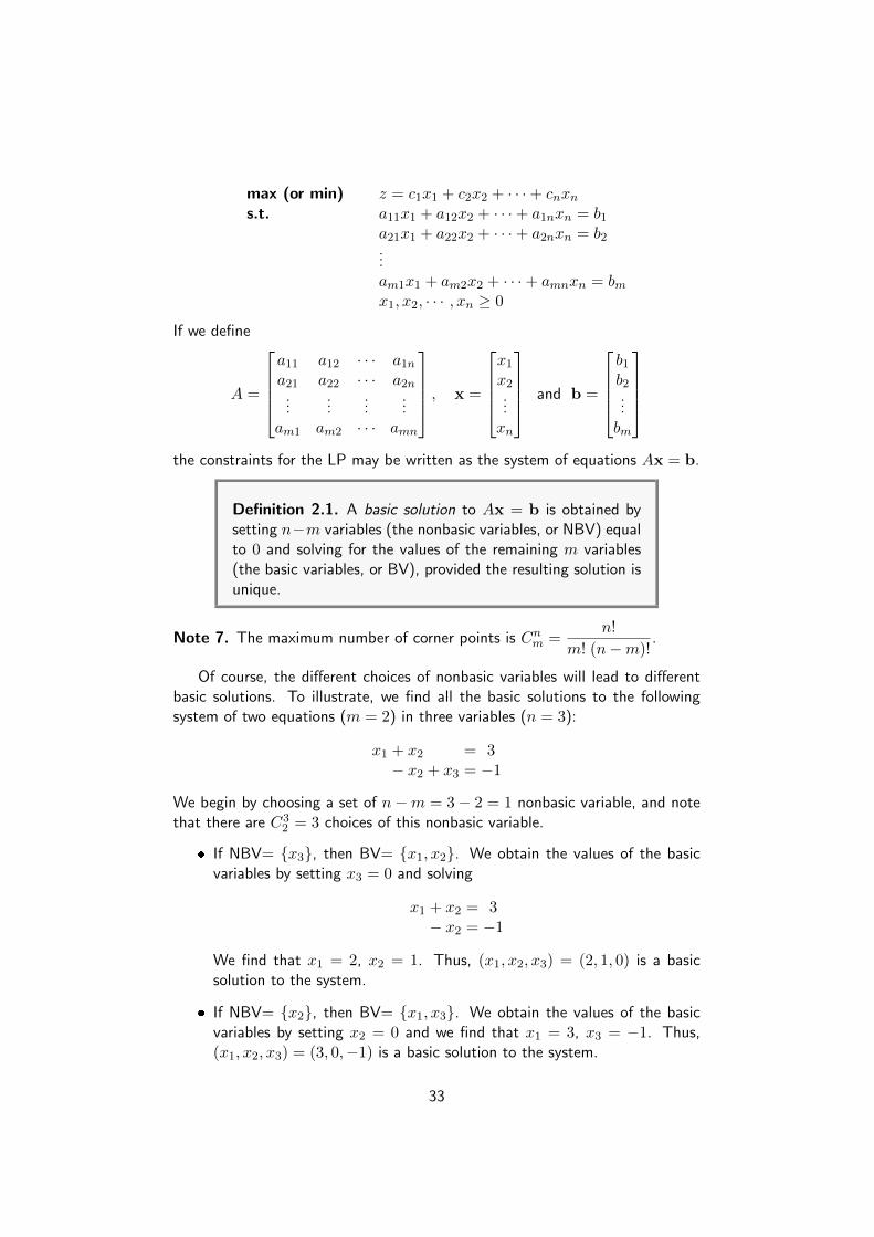
Definition 2.1. A basic solution to Ax = b is obtained bysetting n−m variables (the nonbasic variables, or NBV) equalto 0 and solving for the values of the remaining m variables(the basic variables, or BV), provided the resulting solution isunique.
Note 7. The maximum number of corner points is Cnm =
n!
m! (n−m)!.
Of course, the different choices of nonbasic variables will lead to differentbasic solutions. To illustrate, we find all the basic solutions to the followingsystem of two equations (m = 2) in three variables (n = 3):
x1 + x2 = 3− x2 + x3 = −1
We begin by choosing a set of n−m = 3− 2 = 1 nonbasic variable, and notethat there are C3
2 = 3 choices of this nonbasic variable.
� If NBV= {x3}, then BV= {x1, x2}. We obtain the values of the basicvariables by setting x3 = 0 and solving
x1 + x2 = 3− x2 = −1
We find that x1 = 2, x2 = 1. Thus, (x1, x2, x3) = (2, 1, 0) is a basicsolution to the system.
� If NBV= {x2}, then BV= {x1, x3}. We obtain the values of the basicvariables by setting x2 = 0 and we find that x1 = 3, x3 = −1. Thus,(x1, x2, x3) = (3, 0,−1) is a basic solution to the system.
33

� If NBV= {x1}, then BV= {x2, x3}. We obtain the values of the basicvariables by setting x1 = 0 and solving
x2 = 3− x2 + x3 = −1
We find that x2 = 3, x3 = 2. Thus, (x1, x2, x3) = (0, 3, 2) is a basicsolution to the system.
The following table provides all the basic and nonbasic solutions of the abovelinear system.
NBVs BVs Basic Solution
x1 x2, x3 3, 2x2 x1, x3 3,−1x3 x1, x2 2, 1
Note 8. Some sets of m variables do not yield a basic solution. For example,consider the following linear system:
x1 + 2x2 + x3 = 12x1 + 4x2 + x3 = 3
If we choose NBV= {x3} and BV= {x1, x2}, the corresponding basic solutionwould be obtained by solving
x1 + 2x2 = 12x1 + 4x2 = 3
Because this system has no solution, there is no basic solution corresponding toBV= {x1, x2}.
Definition 2.2. Any basic solution to the constraints Ax = bof an LP in which all variables are nonnegative is a basicfeasible solution (or bfs).
For example, for an LP with the constraints given by
x1 + x2 = 3− x2 + x3 = −1
the basic solutions x1 = 2, x2 = 1, x3 = 0, and x1 = 0, x2 = 3, x3 = 2 arebasic feasible solutions, but the basic solution x1 = 3, x2 = 0, x3 = −1 fails tobe a feasible solution (because x3 < 0).
34

Theorem 2.1. A point in the feasible region of an LP is anextreme point if and only if it is a basic feasible solution tothe LP.
Example 2.2. Consider the following LP with two variables.
max z = 2x1 + 3x2s.t. 2x1 + x2 ≤ 4
x1 + 2x2 ≤ 5x1, x2 ≥ 0
Solution: By adding slack variables s1 and s2, respectively, we obtain the LPin standard form:
max z = 2x1 + 3x2s.t. 2x1 + x2 + s1 = 4
x1 + 2x2 + s2 = 5x1, x2, s1, s2 ≥ 0
Figure 23 provides the graphical solution space for the problem. Algebraically,
Figure 23
the solution space of the LP is represented by the following m = 2 equationsand n = 4 variables:
2x1 + x2 + s1 = 4x1 + 2x2 + s2 = 5
The basic solutions are determined by setting n−m = 2 variables equal to zeroand solving for the remaining m = 2 variables. For example, if we set x1 = 0and x2 = 0, the equations provide the unique basic solution
s1 = 4 and s2 = 5.
35

This solution corresponds to point A in Figure 23. Another point can be de-termined by setting s1 = 0 and s2 = 0 and then solving the resulting twoequations
2x1 + x2 = 4x1 + 2x2 = 5
The associated basic solution is x1 = 1, x2 = 2, or point C in Figure 23. In thepresent example, the maximum number of corner points is C4
2 = 6. Looking atFigure 23, we can spot the four corner points A, B, C, and D. So, where arethe remaining two? In fact, points E and F also are corner points. But, theyare infeasible, and, hence, are not candidates for the optimum. The followingtable provides all the basic and nonbasic solutions of the current example.
Basic CornerNBVs BVs Solution Point Feasible? z−Valuex1, x2 s1, s2 4, 5 A 3 0x1, s1 x2, s2 4,−3 F 7
x1, s2 x2, s1 2.5, 1.5 B 3 7.5x2, s1 x1, s2 2, 3 D 3 4x2, s2 x1, s1 5,−6 E 7
s1, s2 x1, x2 1, 2 C 3 8 Optimum
Exercise 2.2.
1. Consider the following LP:
max z = 2x1 + 3x2s.t. x1 + 3x2 ≤ 12
3x1 + 2x2 ≤ 12x1, x2 ≥ 0
(a) Express the problem in equation form.
(b) Determine all the basic solutions of the problem, and classify themas feasible and infeasible.
(c) Use direct substitution in the objective function to determine theoptimum basic feasible solution.
(d) Verify graphically that the solution obtained in (c) is the optimum LPsolution, hence, conclude that the optimum solution can be deter-mined algebraically by considering the basic feasible solutions only.
(e) Show how the infeasible basic solutions are represented on the graph-ical solution space.
2. Determine the optimum solution for each of the following LPs by enumer-ating all the basic solutions.
36
(a) max z = 2x1 − 4x2 + 5x3 − 6x4s.t. x1 + 5x2 − 2x3 + 8x4 ≤ 2
−x1 + 2x2 + 3x3 + 4x4 ≤ 1x1, x2, x3, x4 ≥ 0
(b) min w = x1 + 2x2 − 3x3 − 2x4s.t. x1 + 2x2 − 3x3 + x4 = 4
x1 + 2x2 + x3 + 2x4 = 4x1, x2, x3, x4 ≥ 0
3. Show algebraically that all the basic solutions of the following LP areinfeasible.
max z = x1 + x2s.t. x1 + 2x2 ≤ 3
2x1 + x2 ≥ 8x1, x2 ≥ 0
4. Consider the following LP:
max z = x1 + 3x2s.t. x1 + x2 ≤ 2
−2x1 + x2 ≤ 4x1 urs, x2 ≥ 0
(a) Determine all the basic feasible solutions of the problem.
(b) Use direct substitution in the objective function to determine thebest basic solution.
(c) Solve the problem graphically, and verify that the solution obtainedin (b) is the optimum.
2.4 The Simplex Algorithm
Rather than enumerating all the basic solutions (corner points) of the LP prob-lem, as we did in example (2.2), the simplex method investigates only a “se-lect few” of these solutions. This section describes the iterative nature of themethod, and provides the computational details of the simplex algorithm.
Before describing the simplex algorithm in general terms, we need to definethe concept of an adjacent basic feasible solution.
Definition 2.3. For any LP with m constraints, two basicfeasible solutions are said to be adjacent if their sets of basicvariables have m− 1 basic variables in common.
37
For example, in Figure 23, two basic feasible solutions will be adjacent if theyhave 2 − 1 = 1 basic variable in common. Thus, the bfs corresponding topoint B in Figure 23 is adjacent to the bfs corresponding to point C but is notadjacent to bfs D. Intuitively, two basic feasible solutions are adjacent if theyboth lie on the same edge of the boundary of the feasible region.
2.4.1 Iterative Nature of the Simplex Method
Figure 23 provides the solution space of the LP of example (2.2). For the sakeof standardizing the algorithm, the simplex method always starts at the originwhere all the decision variables, xi are zero. In Figure 23, point A is the origin(x1 = x2 = 0) and the associated objective value, z, is zero. The logicalquestion now is whether an increase in the values of nonbasic x1 and x2 abovetheir current zero values can improve (increase) the value of z. We can answerthis question by investigating the objective function:
max z = 2x1 + 3x2
An increase in x1 or x2 (or both) above their current zero values will improvethe value of z. The design of the simplex method does not allow simultaneousincreases in variables. Instead, it targets the variables one at a time. Thevariable slated for increase is the one with the largest rate of improvement inz. In the present example, the rate of improvement in the value of z is 2 for x1and 3 for x2. We thus elect to increase x2 (the variable with the largest rate ofimprovement among all nonbasic variables). Figure 23 shows that the value ofx2 must be increased until corner point B is reached (recall that stopping shortof corner point B is not an option because a candidate for the optimum mustbe a corner point). At point B, the simplex method, as will be explained later,will then increase the value of x1 to reach the improved corner point C, whichis the optimum.
The path of the simplex algorithm always connects adjacent corner points.In the present example the path to the optimum is A→ B → C. Each cornerpoint along the path is associated with an iteration. It is important to note thatthe simplex method always moves alongside the edges of the solution space,which means that the method does not cut across the solution space. Forexample, the simplex algorithm cannot go from A to C directly since they arenot adjacent.
2.4.2 Computational Details of the Simplex Algorithm
We now describe how the simplex algorithm can be used to solve LPs in whichthe goal is to maximize the objective function. The solution of minimizationproblems is discussed in Section 2.5. The simplex algorithm proceeds as follows:
Step 1: Convert the LP to standard form. Then, write the objective function
z = c1x1 + c2x2 + · · ·+ cnxn
38

in the formz − c1x1 − c2x2 − · · · − cnxn = 0.
We call this format the row 0 version of the objective function (row 0 forshort).
Step 2: Obtain a bfs (if possible) from the standard form. This is easy if allthe constraints are ≤ with nonnegative right-hand sides. Then the slackvariable si may be used as the basic variable for row i. If no bfs is readilyapparent, then use the technique discussed in Section 2.6 to find a bfs.
Step 3: Determine whether the current bfs is optimal. If all nonbasic variableshave nonnegative coefficients in row 0, then the current bfs is optimal. Ifany variables in row 0 have negative coefficients, then choose the variablewith the most negative coefficient in row 0 to enter the basis. We callthis variable the entering variable.
Step 4: If the current bfs is not optimal, then determine which nonbasic variableshould become a basic variable and which basic variable should become anonbasic variable to find a new bfs with a better objective function value.When entering a variable into the basis, compute the ratio
Right-hand side of constraint
Coefficient of entering variable in constraint
for every constraint in which the entering variable has a positive coeffi-cient. The constraint with the smallest ratio is called the winner of theratio test. The smallest ratio is the largest value of the entering variablethat will keep all the current basic variables nonnegative.
Step 5: Use elementary row operations (EROs) to find the new bfs with thebetter objective function value by making the entering variable a basicvariable (has coefficient 1 in pivot row, and 0 in other rows) in the con-straint that wins the ratio test. Go back to step 3.
2.4.3 Representing the Simplex Tableau
The tabular form of the simplex method records only the essential information:
� the coefficients of the variables,
� the constants on the right-hand sides of the equations,
� the basic variable appearing in each equation.
This saves writing the symbols for the variables in each of the equations, butwhat is even more important is the fact that it permits highlighting the numbers
39
involved in arithmetic calculations and recording the computations compactly.For example, the form
z − 2x1 − 3x2 = 02x1 + x2 + s1 = 4x1 + 2x2 + s2 = 5
would be written in abbreviated form as shown in the following table.
Basic x1 x2 s1 s2 RHS
z −2 −3 0 0 0
s1 2 1 1 0 4s2 1 2 0 1 5
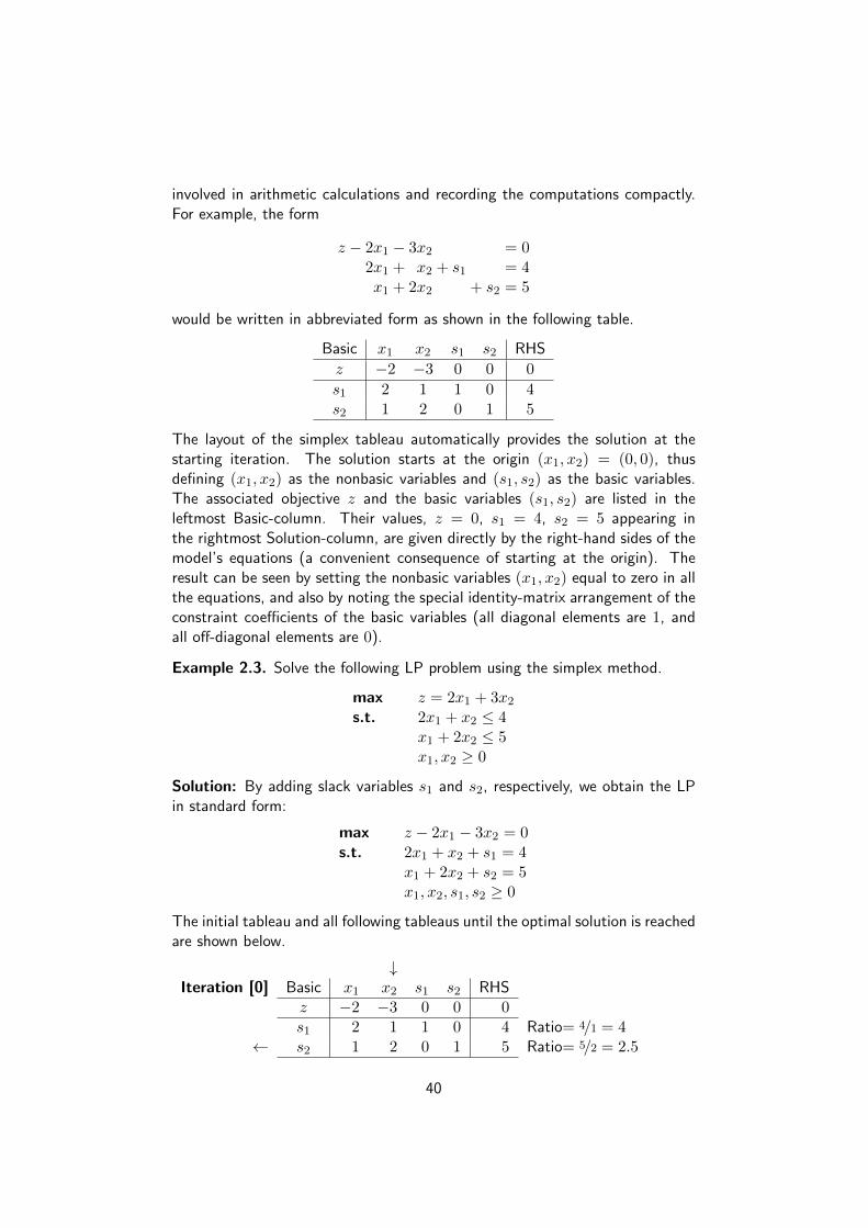
The layout of the simplex tableau automatically provides the solution at thestarting iteration. The solution starts at the origin (x1, x2) = (0, 0), thusdefining (x1, x2) as the nonbasic variables and (s1, s2) as the basic variables.The associated objective z and the basic variables (s1, s2) are listed in theleftmost Basic-column. Their values, z = 0, s1 = 4, s2 = 5 appearing inthe rightmost Solution-column, are given directly by the right-hand sides of themodel’s equations (a convenient consequence of starting at the origin). Theresult can be seen by setting the nonbasic variables (x1, x2) equal to zero in allthe equations, and also by noting the special identity-matrix arrangement of theconstraint coefficients of the basic variables (all diagonal elements are 1, andall off-diagonal elements are 0).
Example 2.3. Solve the following LP problem using the simplex method.
max z = 2x1 + 3x2s.t. 2x1 + x2 ≤ 4
x1 + 2x2 ≤ 5x1, x2 ≥ 0
Solution: By adding slack variables s1 and s2, respectively, we obtain the LPin standard form:
max z − 2x1 − 3x2 = 0s.t. 2x1 + x2 + s1 = 4
x1 + 2x2 + s2 = 5x1, x2, s1, s2 ≥ 0
The initial tableau and all following tableaus until the optimal solution is reachedare shown below.
↓Iteration [0] Basic x1 x2 s1 s2 RHS
z −2 −3 0 0 0s1 2 1 1 0 4 Ratio= 4/1 = 4
← s2 1 2 0 1 5 Ratio= 5/2 = 2.5
40

↓Iteration [1] Basic x1 x2 s1 s2 RHS
z −1/2 0 0 3/2 15/2← s1 3/2 0 1 −1/2 3/2 Ratio= 3/2÷ 3/2 = 1
x2 1/2 1 0 1/2 5/2 Ratio= 5/2÷ 1/2 = 5
Iteration [2] Basic x1 x2 s1 s2 RHS Optimal Tableauz 0 0 1/3 4/3 8 z = 8x1 1 0 2/3 −1/3 1 x1 = 1, x2 = 2x2 0 1 −1/3 2/3 2 s1 = 0, s2 = 0
Example 2.4. Solve the following LP problem using the simplex method.
max z = 4x1 + 4x2s.t. 6x1 + 4x2 ≤ 24
x1 + 2x2 ≤ 6−x1 + x2 ≤ 1x2 ≤ 2x1, x2 ≥ 0
Solution: By adding slack variables s1, s2, s3 and s4, respectively, we obtainthe LP in standard form:
max z − 4x1 − 4x2 = 0s.t. 6x1 + 4x2 + s1 = 24
x1 + 2x2 + s2 = 6−x1 + x2 + s3 = 1x2 + s4 = 2x1, x2, s1, s2, s3, s4 ≥ 0
The initial tableau and all following tableaus until the optimal solution is reachedare shown below. Note that we can choose to enter either x1 or x2 into thebasis. We arbitrarily choose to enter x1 into basis.
↓Iteration [0] Basic x1 x2 s1 s2 s3 s4 RHS
z −4 −4 0 0 0 0 0← s1 6 4 1 0 0 0 24 Ratio= 24/6 = 4
s2 1 2 0 1 0 0 6 Ratio= 6/1 = 6s3 −1 1 0 0 1 0 1 7
s4 0 1 0 0 0 1 2 7
41

↓Iteration [1] Basic x1 x2 s1 s2 s3 s4 RHS
z 0 −4/3 2/3 0 0 0 16x1 1 2/3 1/6 0 0 0 4 Ratio= 4÷ 2/3 = 6
← s2 0 4/3 −1/6 1 0 0 2 Ratio= 2÷ 4/3 = 3/2s3 0 5/3 1/6 0 1 0 5 Ratio= 5÷ 5/3 = 3s4 0 1 0 0 0 1 2 Ratio= 2/1 = 2
Iteration [2] Basic x1 x2 s1 s2 s3 s4 RHS Optimal Tableauz 0 0 1/2 1 0 0 18 z = 18x1 1 0 1/4 −1/2 0 0 3 x1 = 3, x2 = 3/2x2 0 1 −1/8 3/4 0 0 3/2 s1 = 0, s2 = 0s3 0 0 3/8 −5/4 1 0 3/2 s3 = 3/2, s4 = 1/2s4 0 0 1/8 −3/4 0 1 1/2
Example 2.5. Solve the following LP problem using the simplex method.
max z = x1 + 3x2s.t. x1 + x2 ≤ 2
−x1 + x2 ≤ 4x1 ≥ 0, x2 urs
Solution: By assuming x2 = y1 − y2 and then adding slack variables s1 ands2, respectively, we obtain the LP in standard form:
max z − x1 − 3y1 + 3y2 = 0s.t. x1 + y1 − y2 + s1 = 2
−x1 + y1 − y2 + s2 = 4x1, y1, y2, s1, s2 ≥ 0
The initial tableau and all following tableaus until the optimal solution is reachedare shown below.
↓Iteration [0] Basic x1 y1 y2 s1 s2 RHS
z −1 −3 3 0 0 0← s1 1 1 −1 1 0 2 Ratio= 2/1 = 2
s2 −1 1 −1 0 1 4 Ratio= 4/1 = 4
Iteration [1] Basic x1 y1 y2 s1 s2 RHS Optimal Tableauz 2 0 0 3 0 6 z = 6y1 1 1 −1 1 0 2 x1 = 0, x2 = 3s2 −2 0 0 −1 1 2 s1 = 0, s2 = 2
Note that from the optimal tableau we have y1 = 3 and y2 = 0, so thatx2 = y1 − y2 = 3− 0 = 3.
42
Exercise 2.3.
1. Use the simplex algorithm to solve the following problems.
(a) max z = 2x1 + 3x2s.t. x1 + 2x2 ≤ 6
2x1 + x2 ≤ 8x1, x2 ≥ 0
(b) max z = 2x1 − x2 + x3s.t. 3x1 + x2 + x3 ≤ 60
x1 − x2 + 2x3 ≤ 10x1 + x2 − x3 ≤ 20x1, x2, x3 ≥ 0
(c) max z = x1 − x2s.t. 4x1 + x2 ≤ 100
x1 + x2 ≤ 80x1 ≤ 40x1, x2 ≥ 0
(d) max z = x1 + x2 + x3s.t. x1 + 2x2 + 2x3 ≤ 20
2x1 + x2 + 2x3 ≤ 202x1 + 2x2 + x3 ≤ 20x1, x2, x3 ≥ 0
2. Solve the following problem by inspection, and justify the method of so-lution in terms of the basic solutions of the simplex method.
max z = 5x1 − 6x2 + 3x3 − 5x4 + 12x5s.t. x1 + 3x2 + 5x3 + 6x4 + 3x5 ≤ 30
x1, x2, x3, x4, x5 ≥ 0
2.5 Solving Minimization Problem
There are two different ways that the simplex algorithm can be used to solveminimization problems.
Method (1) Multiply the objective function for the min problem by −1 andsolve the problem as a maximization problem with objective function(−w). The optimal solution to the max problem will give you the op-timal solution to the min problem where[
optimal objective functionvalue for min problem
]= −
[optimal objective function
value for max problem
]Example 2.6. Solve the following LP problem using the simplex method.
min w = 2x1 − 3x2s.t. x1 + x2 ≤ 4
x1 − x2 ≤ 6x1, x2 ≥ 0
Solution: The optimal solution to the LP is the point (x1, x2) in thefeasible region for the LP that makes w = 2x1− 3x2 the smallest. Equiv-alently, we may say that the optimal solution to the LP is the point inthe feasible region that makes z = −w = −2x1 + 3x2 the largest. Thismeans that we can find the optimal solution to the LP by solving:
43

max z = −2x1 + 3x2s.t. x1 + x2 ≤ 4
x1 − x2 ≤ 6x1, x2 ≥ 0
By adding slack variables s1 and s2, respectively, we obtain the LP instandard form:
max z + 2x1 − 3x2 = 0s.t. x1 + x2 + s1 = 4
x1 − x2 + s2 = 6x1, x2, s1, s2 ≥ 0
The initial tableau and all following tableaus until the optimal solution isreached are shown below.
↓Iteration [0] Basic x1 x2 s1 s2 RHS
z 2 −3 0 0 0← s1 1 1 1 0 4 Ratio= 4/1 = 4
s2 1 −1 0 1 6 7
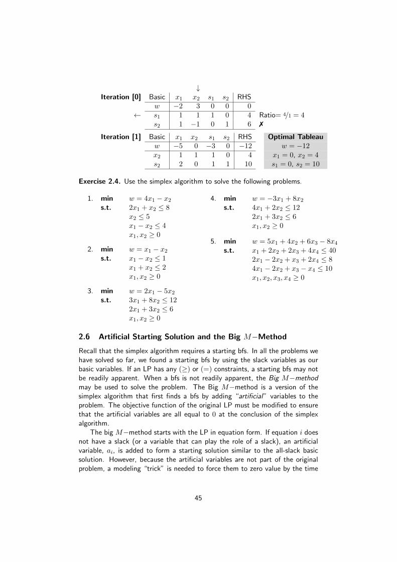
Iteration [1] Basic x1 x2 s1 s2 RHS Optimal Tableauz 5 0 3 0 12 w = −z = −12x2 1 1 1 0 4 x1 = 0, x2 = 4s2 2 0 1 1 10 s1 = 0, s2 = 10
Method (2) A simple modification of the simplex algorithm can be used tosolve min problems directly. Modify Step 3 of the simplex as follows:If all nonbasic variables in row 0 have nonpositive coefficients, then thecurrent bfs is optimal. If any nonbasic variable in row 0 has a positivecoefficient, choose the variable with the “most positive” coefficient in row0 to enter the basis. This modification of the simplex algorithm worksbecause increasing a nonbasic variable with a positive coefficient in row 0will decrease w. If we use this method to solve the LP in example (2.6),then after adding slack variables s1 and s2, respectively, we obtain the LPin standard form:
min w − 2x1 + 3x2 = 0s.t. x1 + x2 + s1 = 4
x1 − x2 + s2 = 6x1, x2, s1, s2 ≥ 0
The initial tableau and all following tableaus until the optimal solution isreached are shown below. Note that, because x2 has the most positivecoefficient in row 0, we enter x2 into the basis.
44
↓Iteration [0] Basic x1 x2 s1 s2 RHS
w −2 3 0 0 0← s1 1 1 1 0 4 Ratio= 4/1 = 4
s2 1 −1 0 1 6 7
Iteration [1] Basic x1 x2 s1 s2 RHS Optimal Tableauw −5 0 −3 0 −12 w = −12x2 1 1 1 0 4 x1 = 0, x2 = 4s2 2 0 1 1 10 s1 = 0, s2 = 10
Exercise 2.4. Use the simplex algorithm to solve the following problems.
1. min w = 4x1 − x2s.t. 2x1 + x2 ≤ 8
x2 ≤ 5x1 − x2 ≤ 4x1, x2 ≥ 0
2. min w = x1 − x2s.t. x1 − x2 ≤ 1
x1 + x2 ≤ 2x1, x2 ≥ 0
3. min w = 2x1 − 5x2s.t. 3x1 + 8x2 ≤ 12
2x1 + 3x2 ≤ 6x1, x2 ≥ 0
4. min w = −3x1 + 8x2s.t. 4x1 + 2x2 ≤ 12
2x1 + 3x2 ≤ 6x1, x2 ≥ 0
5. min w = 5x1 + 4x2 + 6x3 − 8x4s.t. x1 + 2x2 + 2x3 + 4x4 ≤ 40
2x1 − 2x2 + x3 + 2x4 ≤ 84x1 − 2x2 + x3 − x4 ≤ 10x1, x2, x3, x4 ≥ 0
2.6 Artificial Starting Solution and the Big M−Method
Recall that the simplex algorithm requires a starting bfs. In all the problems wehave solved so far, we found a starting bfs by using the slack variables as ourbasic variables. If an LP has any (≥) or (=) constraints, a starting bfs may notbe readily apparent. When a bfs is not readily apparent, the Big M−methodmay be used to solve the problem. The Big M−method is a version of thesimplex algorithm that first finds a bfs by adding “artificial” variables to theproblem. The objective function of the original LP must be modified to ensurethat the artificial variables are all equal to 0 at the conclusion of the simplexalgorithm.
The big M−method starts with the LP in equation form. If equation i doesnot have a slack (or a variable that can play the role of a slack), an artificialvariable, ai, is added to form a starting solution similar to the all-slack basicsolution. However, because the artificial variables are not part of the originalproblem, a modeling “trick” is needed to force them to zero value by the time
45

the optimum iteration is reached (assuming the problem has a feasible solution).The desired goal is achieved by assigning a penalty defined as:
Artificial variable objectivefunction coefficient
=
{−M in max problemsM in min problems
where M is a sufficiently large positive value (mathematically, M →∞).
Example 2.7. Solve the following LP problem using the simplex method.
min w = 4x1 + x2s.t. 3x1 + x2 = 3
4x1 + 3x2 ≥ 6x1 + 2x2 ≤ 4x1, x2 ≥ 0
Solution: To convert the constraint to equations, use e2 as a surplus in thesecond constraint and s3 as a slack in the third constraint.
3x1 + x2 = 34x1 + 3x2 − e2 = 6x1 + 2x2 + s3 = 4
The third equation has its slack variable, s3, but the first and second equationsdo not. Thus, we add the artificial variables a1 and a2 in the first two equationsand penalize them in the objective function with Ma1 + Ma2 (because we areminimizing). The resulting LP becomes
min w = 4x1 + x2 + Ma1 + Ma2s.t. 3x1 + x2 + a1 = 3
4x1 + 3x2 − e2 + a2 = 6x1 + 2x2 + s3 = 4x1, x2, s3, e2, a1, a2 ≥ 0
After writing the objective function as w − 4x1 − x2 −Ma1 −Ma2 = 0, theinitial tableau will be
Iteration [0] Basic x1 x2 s3 e2 a1 a2 RHSw −4 −1 0 0 −M −M 0a1 3 1 0 0 1 0 3a2 4 3 0 −1 0 1 6s3 1 2 1 0 0 0 4
Before proceeding with the simplex method computations, row 0 must be madeconsistent with the rest of the tableau. The right−hand side of row 0 in thetableau currently shows w = 0. However, given the nonbasic solution x1 =x2 = e2 = 0, the current basic solution is a1 = 3, a2 = 6, and s3 = 4 yields
w = (4× 0) + (1× 0) + (3×M) + (6×M) = 9M 6= 0.
46
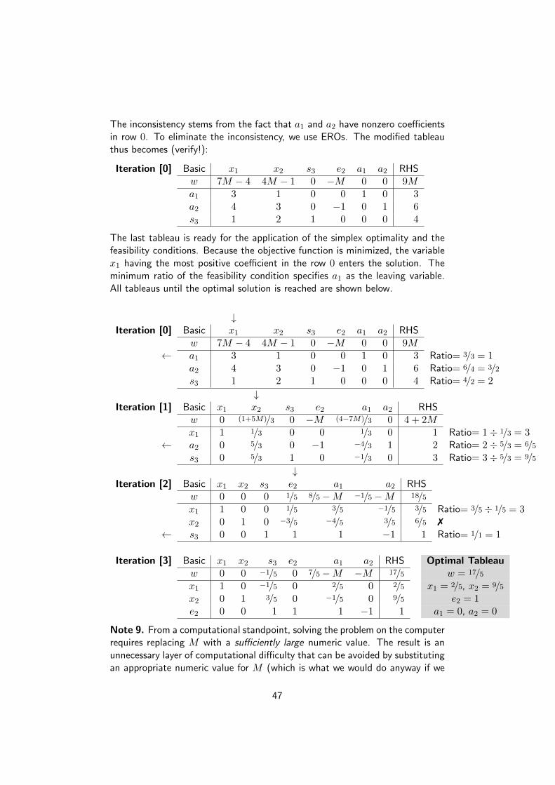
The inconsistency stems from the fact that a1 and a2 have nonzero coefficientsin row 0. To eliminate the inconsistency, we use EROs. The modified tableauthus becomes (verify!):
Iteration [0] Basic x1 x2 s3 e2 a1 a2 RHSw 7M − 4 4M − 1 0 −M 0 0 9Ma1 3 1 0 0 1 0 3a2 4 3 0 −1 0 1 6s3 1 2 1 0 0 0 4
The last tableau is ready for the application of the simplex optimality and thefeasibility conditions. Because the objective function is minimized, the variablex1 having the most positive coefficient in the row 0 enters the solution. Theminimum ratio of the feasibility condition specifies a1 as the leaving variable.All tableaus until the optimal solution is reached are shown below.
↓Iteration [0] Basic x1 x2 s3 e2 a1 a2 RHS
w 7M − 4 4M − 1 0 −M 0 0 9M← a1 3 1 0 0 1 0 3 Ratio= 3/3 = 1
a2 4 3 0 −1 0 1 6 Ratio= 6/4 = 3/2s3 1 2 1 0 0 0 4 Ratio= 4/2 = 2
↓Iteration [1] Basic x1 x2 s3 e2 a1 a2 RHS
w 0 (1+5M)/3 0 −M (4−7M)/3 0 4 + 2Mx1 1 1/3 0 0 1/3 0 1 Ratio= 1÷ 1/3 = 3
← a2 0 5/3 0 −1 −4/3 1 2 Ratio= 2÷ 5/3 = 6/5s3 0 5/3 1 0 −1/3 0 3 Ratio= 3÷ 5/3 = 9/5
↓Iteration [2] Basic x1 x2 s3 e2 a1 a2 RHS
w 0 0 0 1/5 8/5−M −1/5−M 18/5x1 1 0 0 1/5 3/5 −1/5 3/5 Ratio= 3/5÷ 1/5 = 3x2 0 1 0 −3/5 −4/5 3/5 6/5 7
← s3 0 0 1 1 1 −1 1 Ratio= 1/1 = 1
Iteration [3] Basic x1 x2 s3 e2 a1 a2 RHS Optimal Tableauw 0 0 −1/5 0 7/5−M −M 17/5 w = 17/5x1 1 0 −1/5 0 2/5 0 2/5 x1 = 2/5, x2 = 9/5x2 0 1 3/5 0 −1/5 0 9/5 e2 = 1e2 0 0 1 1 1 −1 1 a1 = 0, a2 = 0
Note 9. From a computational standpoint, solving the problem on the computerrequires replacing M with a sufficiently large numeric value. The result is anunnecessary layer of computational difficulty that can be avoided by substitutingan appropriate numeric value for M (which is what we would do anyway if we
47

use the computer). We break away from the long tradition of manipulating Malgebraically and use a numerical substitution instead. The intent is to simplifythe presentation without losing substance. What value of M should we use?The answer depends on the data of the original LP. Recall that the penaltyM must be sufficiently large relative to the original objective coefficients toforce the artificial variables to be zero (which happens only if a feasible solutionexists). At the same time, since computers are the main tool for solving LPs,M should not be unnecessarily too large, as this may lead to serious round-offerror. In the present example, the objective coefficients of x1 and x2 are 2 and1, respectively, and it appears reasonable to set M = 100.
Example 2.8. Solve the following LP problem using the simplex method.
max z = 2x1 + x2s.t. x1 + x2 ≤ 10
−x1 + x2 ≥ 2x1, x2 ≥ 0
Solution: To convert the constraint to equations, use s1 as a slack in the firstconstraint and e2 as a surplus in the second constraint.
x1 + x2 + s1 = 10−x1 + x2 − e2 = 2
We add the artificial variables a2 in the second equation and penalize it in theobjective function with −Ma2 = −100a2 (because we are maximizing). Theresulting LP becomes
max z = 2x1 + x2 − 100a2s.t. x1 + x2 + s1 = 10
−x1 + x2 − e2 + a2 = 2x1, x2, s1, e2, a2 ≥ 0
After writing the objective function as z − 2x1 − x2 + 100a2 = 0, the initialtableau will be
Iteration [0] Basic x1 x2 s1 e2 a2 RHSz −2 −1 0 0 100 0s1 1 1 1 0 0 10a2 −1 1 0 −1 1 2
Before proceeding with the simplex method computations, row 0 must be madeconsistent with the rest of the tableau. The inconsistency stems from the factthat a2 has nonzero coefficients in row 0. To eliminate the inconsistency, we useEROs. The modified tableau and all other tableaus until the optimal solutionis reached are:
48

↓Iteration [0] Basic x1 x2 s1 e2 a2 RHS
z 98 −101 0 100 0 −200s1 1 1 1 0 0 10 Ratio= 10/1 = 10
← a2 −1 1 0 −1 1 2 Ratio= 2/1 = 2
↓Iteration [1] Basic x1 x2 s1 e2 a2 RHS
z −3 0 0 −1 101 2← s1 2 0 1 1 −1 8 Ratio= 8/2 = 4
x2 −1 1 0 −1 1 2 7
Iteration [2] Basic x1 x2 s1 e2 a2 RHS Optimal Tableauz 0 0 3/2 1/2 199/2 14 z = 14x1 1 0 1/2 1/2 −1/2 4 x1 = 4,x2 = 6x2 0 1 1/2 −1/2 1/2 6 s1 = e2 = a2 = 0
Example 2.9. Consider the problem.
max z = 2x1 + 4x2 + 4x3 − 3x4s.t. x1 + x2 + x3 = 4
x1 + 4x2 + x4 = 8x1, x2, x3, x4 ≥ 0
The variables x3 and x4 play the role of slack variables. So, without using any ar-tificial variables, solve the problem with x3 and x4 as the starting basic variables.
Solution: The main difference here from the usual simplex is that x3 and x4have nonzero objective coefficients in row 0: z−2x1−4x2−4x3 +3x4 = 0. Toeliminate their coefficients, we use EROs. The initial tableaus and all followingtableaus until the optimal solution is reached are shown below.
Iteration [0] Basic x1 x2 x3 x4 RHSz −2 −4 −4 3 0x3 1 1 1 0 4x4 1 4 0 1 8
↓Iteration [0] Basic x1 x2 x3 x4 RHS
z −1 −12 0 0 −8x3 1 1 1 0 4 Ratio= 4/1 = 4
← x4 1 4 0 1 8 Ratio= 8/4 = 2
Iteration [1] Basic x1 x2 x3 x4 RHS Optimal Tableauz 2 0 0 3 16 z = 16x3 3/4 0 1 −1/4 2 x1 = 0, x2 = 2x2 1/4 1 0 1/4 2 x3 = 2, x4 = 0
49

Exercise 2.5.
1. Use the Big M -method to solve the following LPs:
(a) min w = 4x1 + 4x2 + x3s.t. x1 + x2 + x3 ≤ 2
2x1 + x2 ≤ 32x1 + x2 + 3x3 ≥ 3x1, x2, x3 ≥ 0
(b) min w = x1 + x2s.t. 2x1 + x2 + x3 = 4
x1 + x2 + 2x3 ≤ 2x1, x2, x3 ≥ 0
(c) min w = 2x1 + 3x2s.t. 2x1 + x2 ≥ 4
x1 − x2 ≥ −1x1, x2 ≥ 0
(d) max z = 3x1 + x2s.t. 2x1 + x2 ≤ 4
x1 + x2 = 3x1, x2 ≥ 0
2. Solve the following problem using x3 and x4 as starting basic feasiblevariables. As in example (2.9), do not use any artificial variables.
min z = 3x1 + 2x2 + 3x3 + 2x4s.t. x1 + 4x2 + x3 ≥ 14
2x1 + x2 + x4 ≥ 20x1, x2, x3, x4 ≥ 0
3. Consider the problem
max z = x1 + 5x2 + 3x3s.t. x1 + 2x2 + x3 = 6
2x1 − x2 = 8x1, x2, x3 ≥ 0
The variable x3 plays the role of a slack. Thus, no artificial variableis needed in the first constraint. In the second constraint, an artificialvariable, a2, is needed. Solve the problem using x3 and a2 as the startingvariables.
2.7 Special Cases in the Simplex Method
This section considers four special cases that arise in the use of the simplexmethod.
2.7.1 Degeneracy
In the application of the feasibility condition of the simplex method, a tie for theminimum ratio may occur and can be broken arbitrarily. When this happens, atleast one basic variable will be zero in the next iteration, and the new solutionis said to be degenerate. This situation may reveal that the model has at leastone redundant constraint.
50

Definition 2.4. An LP is degenerate if it has at least one bfsin which a basic variable is equal to zero.
If one of these degenerate basic variables retains its value of zero until it ischosen at a subsequent iteration to be a leaving basic variable, the correspondingentering basic variable also must remain zero, so the value of the objectivefunction must remain unchanged. However, if the objective function may remainthe same rather than change at each iteration, the simplex method may then goaround in a loop, repeating the same sequence of solutions periodically ratherthan eventually changing the objective function toward an optimal solution.This occurrence is called cycling.
Example 2.10. Solve the following LP problem.
max z = 3x1 + 9x2s.t. x1 + 4x2 ≤ 8
x1 + 2x2 ≤ 4x1, x2 ≥ 0
Solution: By adding slack variables s1 and s2, we obtain the LP in standardform
max z − 3x1 − 9x2 = 0s.t. x1 + 4x2 + s1 = 8
x1 + 2x2 + s2 = 4x1, x2, s1, s2 ≥ 0
The initial tableau and all following tableaus until the optimal solution is reachedare shown below.
↓Iteration [0] Basic x1 x2 s1 s2 RHS
z −3 −9 0 0 0← s1 1 4 1 0 8 Ratio= 8/4 = 2
s2 1 2 0 1 4 Ratio= 4/2 = 2
In iteration 0, s1 and s2 tie for the leaving variable, leading to degeneracy initeration 1 because the basic variable s2 assumes a zero value.
↓Iteration [1] Basic x1 x2 s1 s2 RHS
z −3/4 0 9/4 0 18x2 1/4 1 1/4 0 2 Ratio= 2÷ 1/4 = 8
← s2 1/2 0 −1/2 1 0 Ratio= 0÷ 1/2 = 0
Iteration [2] Basic x1 x2 s1 s2 RHS Optimal Tableauz 0 0 3/2 3/2 18 z = 18x2 0 1 1/2 −1/2 2 x1 = 0, x2 = 2x1 1 0 −1 2 0 s1 = 0, s2 = 0
51
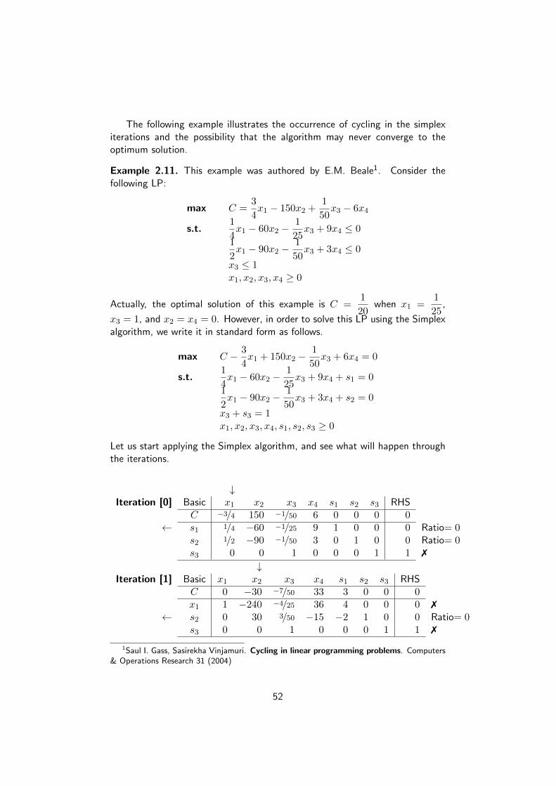
The following example illustrates the occurrence of cycling in the simplexiterations and the possibility that the algorithm may never converge to theoptimum solution.
Example 2.11. This example was authored by E.M. Beale1. Consider thefollowing LP:
max C =3
4x1 − 150x2 +
1
50x3 − 6x4
s.t.1
4x1 − 60x2 −
1
25x3 + 9x4 ≤ 0
1
2x1 − 90x2 −
1
50x3 + 3x4 ≤ 0
x3 ≤ 1x1, x2, x3, x4 ≥ 0
Actually, the optimal solution of this example is C =1
20when x1 =
1
25,
x3 = 1, and x2 = x4 = 0. However, in order to solve this LP using the Simplexalgorithm, we write it in standard form as follows.
max C − 3
4x1 + 150x2 −
1
50x3 + 6x4 = 0
s.t.1
4x1 − 60x2 −
1
25x3 + 9x4 + s1 = 0
1
2x1 − 90x2 −
1
50x3 + 3x4 + s2 = 0
x3 + s3 = 1x1, x2, x3, x4, s1, s2, s3 ≥ 0
Let us start applying the Simplex algorithm, and see what will happen throughthe iterations.
↓Iteration [0] Basic x1 x2 x3 x4 s1 s2 s3 RHS
C −3/4 150 −1/50 6 0 0 0 0← s1 1/4 −60 −1/25 9 1 0 0 0 Ratio= 0
s2 1/2 −90 −1/50 3 0 1 0 0 Ratio= 0s3 0 0 1 0 0 0 1 1 7
↓Iteration [1] Basic x1 x2 x3 x4 s1 s2 s3 RHS
C 0 −30 −7/50 33 3 0 0 0x1 1 −240 −4/25 36 4 0 0 0 7
← s2 0 30 3/50 −15 −2 1 0 0 Ratio= 0s3 0 0 1 0 0 0 1 1 7
1Saul I. Gass, Sasirekha Vinjamuri. Cycling in linear programming problems. Computers& Operations Research 31 (2004)
52
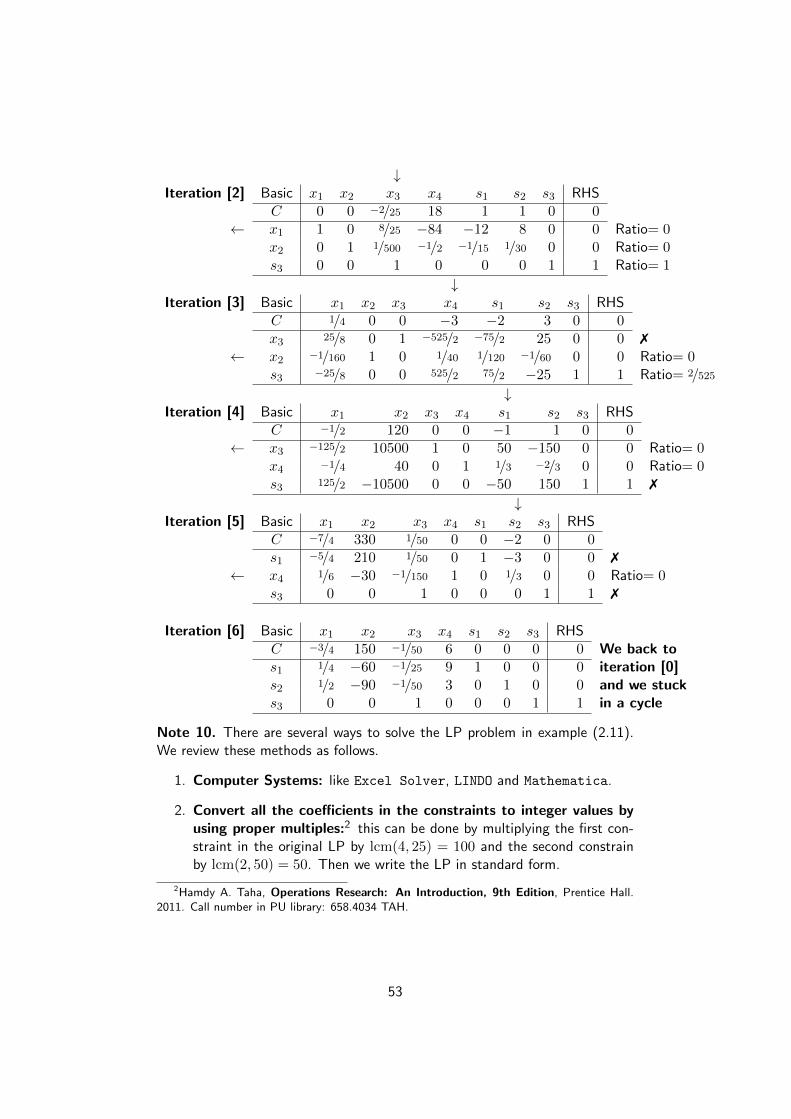
↓Iteration [2] Basic x1 x2 x3 x4 s1 s2 s3 RHS
C 0 0 −2/25 18 1 1 0 0← x1 1 0 8/25 −84 −12 8 0 0 Ratio= 0
x2 0 1 1/500 −1/2 −1/15 1/30 0 0 Ratio= 0s3 0 0 1 0 0 0 1 1 Ratio= 1
↓Iteration [3] Basic x1 x2 x3 x4 s1 s2 s3 RHS
C 1/4 0 0 −3 −2 3 0 0x3 25/8 0 1 −525/2 −75/2 25 0 0 7
← x2 −1/160 1 0 1/40 1/120 −1/60 0 0 Ratio= 0s3 −25/8 0 0 525/2 75/2 −25 1 1 Ratio= 2/525
↓Iteration [4] Basic x1 x2 x3 x4 s1 s2 s3 RHS
C −1/2 120 0 0 −1 1 0 0← x3 −125/2 10500 1 0 50 −150 0 0 Ratio= 0
x4 −1/4 40 0 1 1/3 −2/3 0 0 Ratio= 0s3 125/2 −10500 0 0 −50 150 1 1 7
↓Iteration [5] Basic x1 x2 x3 x4 s1 s2 s3 RHS
C −7/4 330 1/50 0 0 −2 0 0s1 −5/4 210 1/50 0 1 −3 0 0 7
← x4 1/6 −30 −1/150 1 0 1/3 0 0 Ratio= 0s3 0 0 1 0 0 0 1 1 7
Iteration [6] Basic x1 x2 x3 x4 s1 s2 s3 RHSC −3/4 150 −1/50 6 0 0 0 0 We back tos1 1/4 −60 −1/25 9 1 0 0 0 iteration [0]s2 1/2 −90 −1/50 3 0 1 0 0 and we stucks3 0 0 1 0 0 0 1 1 in a cycle
Note 10. There are several ways to solve the LP problem in example (2.11).We review these methods as follows.
1. Computer Systems: like Excel Solver, LINDO and Mathematica.
2. Convert all the coefficients in the constraints to integer values byusing proper multiples:2 this can be done by multiplying the first con-straint in the original LP by lcm(4, 25) = 100 and the second constrainby lcm(2, 50) = 50. Then we write the LP in standard form.
2Hamdy A. Taha, Operations Research: An Introduction, 9th Edition, Prentice Hall.2011. Call number in PU library: 658.4034 TAH.
53

max C − 3
4x1 + 150x2 −
1
50x3 + 6x4 = 0
s.t. 25x1 − 6000x2 − 4x3 + 900x4 + s1 = 025x1 − 4500x2 − x3 + 150x4 + s2 = 0x3 + s3 = 1x1, x2, x3, x4, s1, s2, s3 ≥ 0
Now we apply the Simplex algorithm.
↓Iteration [0] Basic x1 x2 x3 x4 s1 s2 s3 RHS
C −3/4 150 −1/50 6 0 0 0 0← s1 25 −6000 −4 900 1 0 0 0 Ratio= 0
s2 25 −4500 −1 150 0 1 0 0 Ratio= 0s3 0 0 1 0 0 0 1 1 7
↓Iteration [1] Basic x1 x2 x3 x4 s1 s2 s3 RHS
C 0 −30 −7/50 33 3/100 0 0 0x1 1 −240 −4/25 36 1/25 0 0 0 7
← s2 0 1500 3 −750 −1 1 0 0 Ratio= 0s3 0 0 1 0 0 0 1 1 7
↓Iteration [2] Basic x1 x2 x3 x4 s1 s2 s3 RHS
C 0 0 −2/25 18 1/100 1/50 0 0x1 1 0 8/25 −84 −3/25 4/25 0 0 Ratio= 0
← x2 0 1 1/500 −1/2 −1/1500 1/1500 0 0 Ratio= 0s3 0 0 1 0 0 0 1 1 Ratio= 1
↓Iteration [3] Basic x1 x2 x3 x4 s1 s2 s3 RHS
C 0 40 0 −2 −1/60 7/150 0 0x1 1 −160 0 −4 −1/75 4/75 0 0 7
x3 0 500 1 −250 −1/3 1/3 0 0 7
← s3 0 −500 0 250 1/3 −1/3 1 1 Ratio= 1/250
↓Iteration [4] Basic x1 x2 x3 x4 s1 s2 s3 RHS
C 0 36 0 0 −7/500 11/250 1/125 1/125x1 1 −168 0 0 −1/125 6/125 2/125 2/125 7
x3 0 0 1 0 0 0 1 1 7
← x4 0 −2 0 1 1/750 −1/750 1/250 1/250 Ratio= 3
54

Iteration [5] Basic x1 x2 x3 x4 s1 s2 s3 RHS OptimalC 0 15 0 21/2 0 3/100 1/20 1/20 Tableaux1 1 −180 0 6 0 1/25 1/25 1/25x3 0 0 1 0 0 0 1 1s1 0 −1500 0 750 1 −1 3 3
3. Bland’s Rule for selecting entering and leaving variables3.
(a) For the entering basic variable: Of all negative coefficients in theobjective row (Row 0), choose the one with smallest subscript.
(b) For the departing basic variable: When there is a tie between oneor more ratios computed, choose the candidate for departing basicvariable that has the smallest subscript.
When we use Bland’s rule to solve the LP in example (2.11), we namethe slake variables s1, s2, s3 as x5, x6, x7 respectively. The iterations willbe as follows.
↓Iteration [0] Basic x1 x2 x3 x4 x5 x6 x7 RHS
C −3/4 150 −1/50 6 0 0 0 0← x5 1/4 −60 −1/25 9 1 0 0 0 Ratio= 0
x6 1/2 −90 −1/50 3 0 1 0 0 Ratio= 0x7 0 0 1 0 0 0 1 1 7
↓Iteration [1] Basic x1 x2 x3 x4 x5 x6 x7 RHS
C 0 −30 −7/50 33 3 0 0 0x1 1 −240 −4/25 36 4 0 0 0 7
← x6 0 30 3/50 −15 −2 1 0 0 Ratio= 0x7 0 0 1 0 0 0 1 1 7
↓Iteration [2] Basic x1 x2 x3 x4 x5 x6 x7 RHS
C 0 0 −2/25 18 1 1 0 0← x1 1 0 8/25 −84 −12 8 0 0 Ratio= 0
x2 0 1 1/500 −1/2 −1/15 1/30 0 0 Ratio= 0x7 0 0 1 0 0 0 1 1 Ratio= 1
3James Calvert and William Voxman, Linear Programming, 1st Edition, Harcourt BraceJovanovich Publishers, 1989.
55

↓Iteration [3] Basic x1 x2 x3 x4 x5 x6 x7 RHS
C 1/4 0 0 −3 −2 3 0 0x3 25/8 0 1 −525/2 −75/2 25 0 0 7
← x2 −1/160 1 0 1/40 1/120 −1/60 0 0 Ratio= 0x7 −25/8 0 0 525/2 75/2 −25 1 1 Ratio= 2/525
↓Iteration [4] Basic x1 x2 x3 x4 x5 x6 x7 RHS
C −1/2 120 0 0 −1 1 0 0x3 −125/2 10500 1 0 50 −150 0 0 7
x4 −1/4 40 0 1 1/3 −2/3 0 0 7
← x7 125/2 −10500 0 0 −50 150 1 1 Ratio= 2/125
↓Iteration [5] Basic x1 x2 x3 x4 x5 x6 x7 RHS
C 0 36 0 0 −7/5 11/5 1/125 1/125x3 0 0 1 0 0 0 1 1 7
← x4 0 −2 0 1 2/15 −1/15 1/250 1/250 Ratio= 100/3x1 1 −168 0 0 −4/5 12/5 2/125 2/125 7
Iteration [6] Basic x1 x2 x3 x4 x5 x6 x7 RHS OptimalC 0 15 0 21/2 0 3/2 1/20 1/20 Tableaux3 0 0 1 0 0 0 1 1x5 0 −15 0 15/2 1 −1/2 3/100 3/100x1 1 −180 0 6 0 2 1/25 1/25
4. Lexicographic Rule for selecting an exiting variable4.Given a basic feasible solution with basis B, suppose that the nonbasicvariable xk is chosen to enter the basis (the most negative value in Row0 for maximization LP). The index r of the variable xB leaving the basisis determined as follows. Let
I0 =
{r :
bryrk
= min0≤i≤m
{biyik
: yik > 0
}}If I0 is a singleton, namely I0 = {r}, then xBr leaves the basis. Otherwise,form I1 as follows:
I1 =
{r :
yr1yrk
= mini∈I0
{yi1yik
}}where y∗1 is the first column of the m × m identity matrix. If I1 issingleton, namely, I1 = {r}, then xBr leaves the basis. Otherwise, form
4 Mokhtar S. Bazaraa, John J. Jarvis, Hanif D. Sher, Linear Programming and NetworkFlows, 4th Edition, John Wiley & Sons, Inc. 2010. Call number in PU library: 519.72 BAZ
56
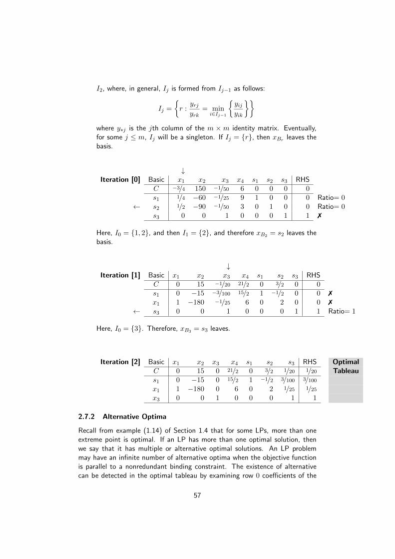
I2, where, in general, Ij is formed from Ij−1 as follows:
Ij =
{r :
yrjyrk
= mini∈Ij−1
{yijyik
}}where y∗j is the jth column of the m × m identity matrix. Eventually,for some j ≤ m, Ij will be a singleton. If Ij = {r}, then xBr leaves thebasis.
↓Iteration [0] Basic x1 x2 x3 x4 s1 s2 s3 RHS
C −3/4 150 −1/50 6 0 0 0 0s1 1/4 −60 −1/25 9 1 0 0 0 Ratio= 0
← s2 1/2 −90 −1/50 3 0 1 0 0 Ratio= 0s3 0 0 1 0 0 0 1 1 7
Here, I0 = {1, 2}, and then I1 = {2}, and therefore xB2 = s2 leaves thebasis.
↓Iteration [1] Basic x1 x2 x3 x4 s1 s2 s3 RHS
C 0 15 −1/20 21/2 0 3/2 0 0s1 0 −15 −3/100 15/2 1 −1/2 0 0 7
x1 1 −180 −1/25 6 0 2 0 0 7
← s3 0 0 1 0 0 0 1 1 Ratio= 1
Here, I0 = {3}. Therefore, xB3 = s3 leaves.
Iteration [2] Basic x1 x2 x3 x4 s1 s2 s3 RHS OptimalC 0 15 0 21/2 0 3/2 1/20 1/20 Tableaus1 0 −15 0 15/2 1 −1/2 3/100 3/100x1 1 −180 0 6 0 2 1/25 1/25x3 0 0 1 0 0 0 1 1
2.7.2 Alternative Optima
Recall from example (1.14) of Section 1.4 that for some LPs, more than oneextreme point is optimal. If an LP has more than one optimal solution, thenwe say that it has multiple or alternative optimal solutions. An LP problemmay have an infinite number of alternative optima when the objective functionis parallel to a nonredundant binding constraint. The existence of alternativecan be detected in the optimal tableau by examining row 0 coefficients of the
57

nonbasic variables. The zero coefficient of nonbasic xj indicates that xj canbe made basic, altering the values of the basic variables without changing thevalue of z.
In practice, alternative optima are useful because we can choose from manysolutions without experiencing deterioration in the objective value. If the exam-ple represents a product-mix situation, it may be advantageous to market twoproducts instead of one.
Example 2.12. Solve the following LP problem.
max z = 2x1 + 4x2s.t. x1 + 2x2 ≤ 5
x1 + x2 ≤ 4x1, x2 ≥ 0
Solution: By adding slack variables s1 and s2, we obtain the LP in standardform
max z − 2x1 − 4x2 = 0s.t. x1 + 2x2 + s1 = 5
x1 + x2 + s2 = 4x1, x2, s1, s2 ≥ 0
The initial tableau and all following tableaus until the optimal solution is reachedare shown below.
↓Iteration [0] Basic x1 x2 s1 s2 RHS
z −2 −4 0 0 0← s1 1 2 1 0 5 Ratio= 5/2
s2 1 1 0 1 4 Ratio= 4/1 = 4
↓Iteration [1] Basic x1 x2 s1 s2 RHS Optimal
z 0 0 2 0 10 Tableaux2 1/2 1 1/2 0 5/2 Ratio= 5/2÷ 1/2 = 5
← s2 1/2 0 −1/2 1 3/2 Ratio= 3/2÷ 3/2 = 3
Iteration [2] Basic x1 x2 s1 s2 RHS Alternativez 0 0 2 0 10 Optimax2 0 1 1 −1 1x1 1 0 −1 2 3
Mathematically, we can determine all the points (x1, x2) on the line segmentjoining the optimal solutions
(0, 52)
and (3, 1) as follows:
x1 = t(0) + (1− t)(3) = 3− 3tx2 = t
(52
)+ (1− t)(1) = 1 + 3t
2
}; 0 ≤ t ≤ 1
58

2.7.3 Unbounded Solutions
In some LP models, as in example (1.16) of Section 1.4, the solution space isunbounded in at least one variable, meaning that variables may be increasedindefinitely without violating any of the constraints. The associated objectivevalue may also be unbounded in this case. An unbounded LP for a max problemoccurs when a variable with a negative coefficient (positive for min LP) in row0 has a nonpositive coefficient in each constraint.
An unbounded solution space may signal that the model is poorly con-structed. The most likely irregularity in such models is that some key con-straints have not been accounted for. Another possibility is that estimates ofthe constraint coefficients may not be accurate.
Example 2.13. Solve the following LP problem.
max z = 2x1 + x2s.t. x1 − x2 ≤ 10
2x1 ≤ 40x1, x2 ≥ 0
Solution: By adding slack variables s1 and s2, we obtain the LP in standardform
max z − 2x1 − x2 = 0s.t. x1 − x2 + s1 = 10
2x1 + s2 = 40x1, x2, s1, s2 ≥ 0
The initial tableau and all following tableaus until the optimal solution is reachedare shown below.
Iteration [0] Basic x1 x2 s1 s2 RHSz −2 −1 0 0 0s1 1 −1 1 0 10s2 2 0 0 1 40
In the starting tableau, both x1 and x2 have negative z−equation coefficients,meaning that an increase in their values will increase the objective value. Al-though x1 should be the entering variable (it has the most negative z−coefficient),we note that all the constraint coefficients under x2 are ≤ 0, meaning that x2can be increased indefinitely without violating any of the constraints. The resultis that z can be increased indefinitely.
2.7.4 Nonexisting (or Infeasible) Solutions
LP models with inconsistent constraints have no feasible solution, see example(1.15) of Section 1.4. This situation does not occur if all the constraints are
59

of the type ≤ with nonnegative right-hand sides because the slacks providean obvious feasible solution. For other types of constraints, penalized artificialvariables are used to start the solution. If at least one artificial variable ispositive in the optimum iteration, then the LP has no feasible solution. Fromthe practical standpoint, an infeasible space points to the possibility that themodel is not formulated correctly.
Example 2.14. Solve the following LP problem.
max z = 3x1 + 2x2s.t. 2x1 + x2 ≤ 2
3x1 + 4x2 ≥ 12x1, x2 ≥ 0
Solution: To convert the constraint to equations, use s1 as a slack in the firstconstraint and e2 as a surplus in the second constraint.
2x1 + x2 + s1 = 23x1 + 4x2 − e2 = 12
We add the artificial variables a2 in the second equation and penalize it in theobjective function with −Ma2 = −100a2 (because we are maximizing). Theresulting LP becomes
max z = 3x1 + 2x2 − 100a2s.t. 2x1 + x2 + s1 = 2
3x1 + 4x2 − e2 + a2 = 12x1, x2, s1, e2, a2 ≥ 0
After writing the objective function as z − 3x1 − 2x2 + 100a2 = 0, the initialtableau will be and all following tableaus until the optimal solution is reachedare shown below.
Iteration [0] Basic x1 x2 s1 e2 a2 RHS
z −3 −2 0 0 100 0s1 2 1 1 0 0 2a2 3 4 0 −1 1 12
↓Iteration [0] Basic x1 x2 s1 e2 a2 RHS
z −303 −402 0 100 0 −1200← s1 2 1 1 0 0 2 Ratio= 2/1 = 2
a2 3 4 0 −1 1 12 Ratio= 12/4 = 3
Iteration [1] Basic x1 x2 s1 e2 a2 RHS Optimalz 501 0 402 100 0 −396 Tableaux2 2 1 1 0 0 2a2 −5 0 −4 −1 1 4
60

Optimum iteration 1 shows that the artificial variable a2 is positive (= 4),meaning that the LP is infeasible. The result is what we may call a pseudo-optimal solution.
Exercise 2.6.
1. Consider the following LP:
max z = 3x1 + 2x2s.t. 4x1 − x2 ≤ 4
4x1 + 3x2 ≤ 64x1 + x2 ≤ 4x1, x2 ≥ 0
(a) Show that the associated simplex iterations are temporarily degen-erate. How many iterations are needed to reach the optimum?
(b) Verify the result by solving the problem graphically.
(c) Interchange constraints (1) and (3) and resolve the problem. Howmany iterations are needed to solve the problem?
2. Solve the following problem, using the lexicographic rule for noncycling.Repeat using Bland’s Rule:
max z = x1 + 2x2 + x3s.t. x1 + 4x2 + 3x3 ≤ 4
−x1 + x2 + 4x3 ≤ 1x1 + 3x2 + x3 ≤ 6x1, x2, x3 ≥ 0
3. For the following LP, identify three alternative optimal basic solutions.
max z = x1 + 2x2 + 3x3s.t. x1 + 2x2 + 3x3 ≤ 10
x1 + x2 ≤ 5x1 ≤ 1x1, x2, x3 ≥ 0
4. Solve the following LP:
max z = 2x1 − x2 + 3x3s.t. x1 − x2 + 5x3 ≤ 5
2x1 − x2 + 3x3 ≤ 20x1, x2, x3 ≥ 0
From the optimal tableau, show that all the alternative optima are notcorner points (i.e., nonbasic).
61
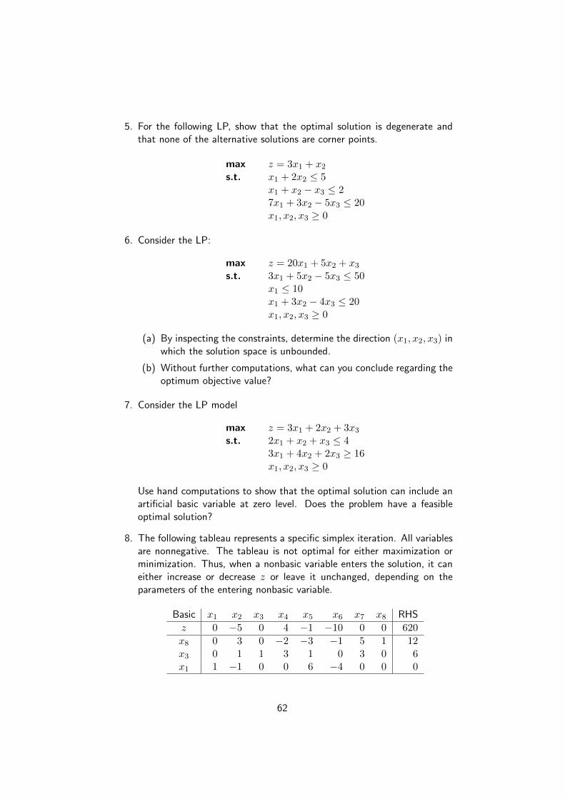
5. For the following LP, show that the optimal solution is degenerate andthat none of the alternative solutions are corner points.
max z = 3x1 + x2s.t. x1 + 2x2 ≤ 5
x1 + x2 − x3 ≤ 27x1 + 3x2 − 5x3 ≤ 20x1, x2, x3 ≥ 0
6. Consider the LP:
max z = 20x1 + 5x2 + x3s.t. 3x1 + 5x2 − 5x3 ≤ 50
x1 ≤ 10x1 + 3x2 − 4x3 ≤ 20x1, x2, x3 ≥ 0
(a) By inspecting the constraints, determine the direction (x1, x2, x3) inwhich the solution space is unbounded.
(b) Without further computations, what can you conclude regarding theoptimum objective value?
7. Consider the LP model
max z = 3x1 + 2x2 + 3x3s.t. 2x1 + x2 + x3 ≤ 4
3x1 + 4x2 + 2x3 ≥ 16x1, x2, x3 ≥ 0
Use hand computations to show that the optimal solution can include anartificial basic variable at zero level. Does the problem have a feasibleoptimal solution?
8. The following tableau represents a specific simplex iteration. All variablesare nonnegative. The tableau is not optimal for either maximization orminimization. Thus, when a nonbasic variable enters the solution, it caneither increase or decrease z or leave it unchanged, depending on theparameters of the entering nonbasic variable.
Basic x1 x2 x3 x4 x5 x6 x7 x8 RHS
z 0 −5 0 4 −1 −10 0 0 620
x8 0 3 0 −2 −3 −1 5 1 12x3 0 1 1 3 1 0 3 0 6x1 1 −1 0 0 6 −4 0 0 0
62
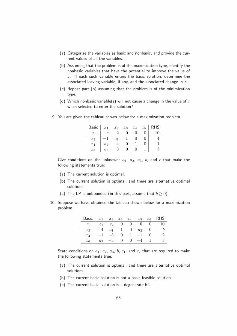
(a) Categorize the variables as basic and nonbasic, and provide the cur-rent values of all the variables.
(b) Assuming that the problem is of the maximization type, identify thenonbasic variables that have the potential to improve the value ofz. If each such variable enters the basic solution, determine theassociated leaving variable, if any, and the associated change in z.
(c) Repeat part (b) assuming that the problem is of the minimizationtype.
(d) Which nonbasic variable(s) will not cause a change in the value of zwhen selected to enter the solution?
9. You are given the tableau shown below for a maximization problem.
Basic x1 x2 x3 x4 x5 RHS
z −c 2 0 0 0 10
x3 −1 a1 1 0 0 4x4 a2 −4 0 1 0 1x5 a3 3 0 0 1 b
Give conditions on the unknowns a1, a2, a3, b, and c that make thefollowing statements true:
(a) The current solution is optimal.
(b) The current solution is optimal, and there are alternative optimalsolutions.
(c) The LP is unbounded (in this part, assume that b ≥ 0).
10. Suppose we have obtained the tableau shown below for a maximizationproblem.
Basic x1 x2 x3 x4 x5 x6 RHS
z c1 c2 0 0 0 0 10
x3 4 a1 1 0 a2 0 bx4 −1 −5 0 1 −1 0 2x6 a3 −3 0 0 −4 1 3
State conditions on a1, a2, a3, b, c1, and c2 that are required to makethe following statements true:
(a) The current solution is optimal, and there are alternative optimalsolutions.
(b) The current basic solution is not a basic feasible solution.
(c) The current basic solution is a degenerate bfs.
63

(d) The current basic solution is feasible, but the LP is unbounded.
(e) The current basic solution is feasible, but the objective function valuecan be improved by replacing x6 as a basic variable with x1.
11. The starting and current tableaux of a given problem are shown below.Find the values of the unknowns a through n.
Starting Basic x1 x2 x3 x4 x5 RHSTableau z a 1 −3 0 0 0
x4 b c d 1 0 6x5 −1 2 e 0 1 1
Current Basic x1 x2 x3 x4 x5 RHSTableau z 0 −1/3 j k ` n
x1 g 2/3 2/3 2/3 0 fx5 h i −1/3 2/3 1 m
64
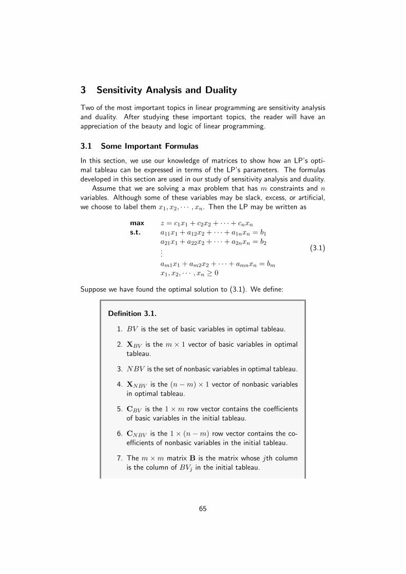
3 Sensitivity Analysis and Duality
Two of the most important topics in linear programming are sensitivity analysisand duality. After studying these important topics, the reader will have anappreciation of the beauty and logic of linear programming.
3.1 Some Important Formulas
In this section, we use our knowledge of matrices to show how an LP’s opti-mal tableau can be expressed in terms of the LP’s parameters. The formulasdeveloped in this section are used in our study of sensitivity analysis and duality.
Assume that we are solving a max problem that has m constraints and nvariables. Although some of these variables may be slack, excess, or artificial,we choose to label them x1, x2, · · · , xn. Then the LP may be written as
max z = c1x1 + c2x2 + · · ·+ cnxns.t. a11x1 + a12x2 + · · ·+ a1nxn = b1
a21x1 + a22x2 + · · ·+ a2nxn = b2...am1x1 + am2x2 + · · ·+ amnxn = bmx1, x2, · · · , xn ≥ 0
(3.1)
Suppose we have found the optimal solution to (3.1). We define:
Definition 3.1.
1. BV is the set of basic variables in optimal tableau.
2. XBV is the m × 1 vector of basic variables in optimaltableau.
3. NBV is the set of nonbasic variables in optimal tableau.
4. XNBV is the (n −m) × 1 vector of nonbasic variablesin optimal tableau.
5. CBV is the 1 ×m row vector contains the coefficientsof basic variables in the initial tableau.
6. CNBV is the 1 × (n −m) row vector contains the co-efficients of nonbasic variables in the initial tableau.
7. The m ×m matrix B is the matrix whose jth columnis the column of BVj in the initial tableau.
65
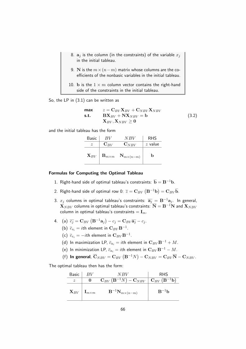
8. aj is the column (in the constraints) of the variable xjin the initial tableau.
9. N is the m× (n−m) matrix whose columns are the co-efficients of the nonbasic variables in the initial tableau.
10. b is the 1 ×m column vector contains the right-handside of the constraints in the initial tableau.
So, the LP in (3.1) can be written as
max z = CBV XBV + CNBV XNBV
s.t. BXBV + NXNBV = bXBV ,XNBV ≥ 0
(3.2)
and the initial tableau has the form
Basic BV NBV RHS
z CBV CNBV z value
XBV Bm×m Nm×(n−m) b
Formulas for Computing the Optimal Tableau
1. Right-hand side of optimal tableau’s constraints: b = B−1b.
2. Right-hand side of optimal row 0: z = CBV
(B−1b
)= CBV b.
3. xj columns in optimal tableau’s constraints: aj = B−1aj . In general,XNBV columns in optimal tableau’s constraints: N = B−1N and XNBV
column in optimal tableau’s constraints = Im.
4. (a) cj = CBV
(B−1aj
)− cj = CBV aj − cj .
(b) csi = ith element in CBV B−1.
(c) cei = −ith element in CBV B−1.
(d) In maximization LP, cai = ith element in CBV B−1 + M .
(e) In minimization LP, cai = ith element in CBV B−1 −M .
(f) In general, CNBV = CBV
(B−1N
)−CNBV = CBV N−CNBV .
The optimal tableau then has the form:
Basic BV NBV RHS
z 0 CBV
(B−1N
)−CNBV CBV
(B−1b
)XBV Im×m B−1Nm×(n−m) B−1b
66

Formulas Derivation:
1. To expressing the constraints in any tableau in terms of B−1 and theoriginal LP, we observe that
BXBV + NXNBV = b
Multiplying both sides from the left by B−1, we obtain
B−1BXBV + B−1NXNBV = B−1b
which implies that
XBV + B−1NXNBV = B−1b
2. To determining the optimal tableau’s Row 0 in terms of the initial LP, werewrite the original objective function, z = CBV XBV + CNBV XNBV as
z −CBV XBV −CNBV XNBV = 0 (3.3)
Also, we multiply the constraints expressed in the form BXBV +NXNBV =b through by the vector CBV B
−1 to obtain
CBV XBV + CBV B−1NXNBV = CBV B
−1b (3.4)
By adding equation (3.3) to equation (3.4), we obtain
z +(CBV B
−1N−CNBV
)XNBV = CBV B
−1b
Example 3.1. For the following LP, the optimal basis is BV = {x2, s2}. Com-pute the optimal tableau.
max z = x1 + 4x2s.t. x1 + 2x2 ≤ 6
2x1 + x2 ≤ 8x1, x2 ≥ 0
Solution: After adding slack variables s1 and s2, the LP in standard form
max z = x1 + 4x2s.t. x1 + 2x2 + s1 = 6
2x1 + x2 + s2 = 8x1, x2, s1, s2 ≥ 0
Since BV = {x2, s2} and NBV = {x1, s1}, then
CBV =[4 0
], CNBV =
[1 0
], b =
[68
]B =
[2 01 1
], B−1 =
[1/2 0−1/2 1
], N =
[1 12 0
]67
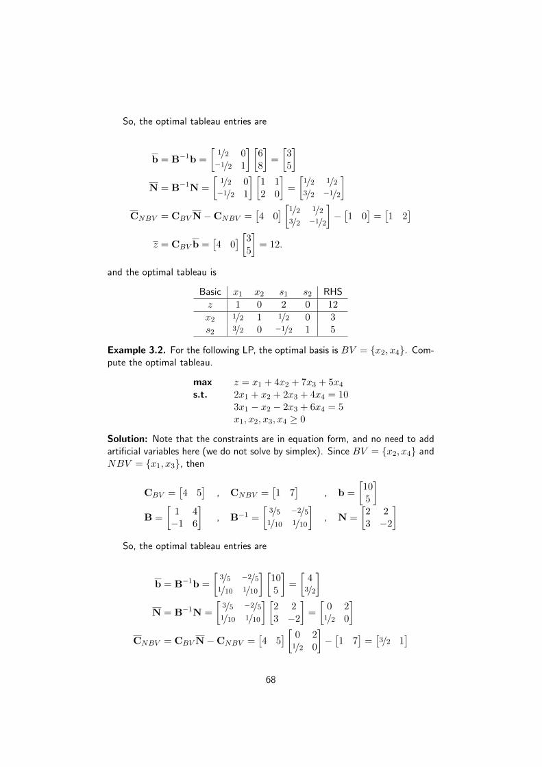
So, the optimal tableau entries are
b = B−1b =
[1/2 0−1/2 1
] [68
]=
[35
]N = B−1N =
[1/2 0−1/2 1
] [1 12 0
]=
[1/2 1/23/2 −1/2
]CNBV = CBV N−CNBV =
[4 0
] [1/2 1/23/2 −1/2
]−[1 0
]=[1 2
]z = CBV b =
[4 0
] [35
]= 12.
and the optimal tableau is
Basic x1 x2 s1 s2 RHS
z 1 0 2 0 12
x2 1/2 1 1/2 0 3s2 3/2 0 −1/2 1 5
Example 3.2. For the following LP, the optimal basis is BV = {x2, x4}. Com-pute the optimal tableau.
max z = x1 + 4x2 + 7x3 + 5x4s.t. 2x1 + x2 + 2x3 + 4x4 = 10
3x1 − x2 − 2x3 + 6x4 = 5x1, x2, x3, x4 ≥ 0
Solution: Note that the constraints are in equation form, and no need to addartificial variables here (we do not solve by simplex). Since BV = {x2, x4} andNBV = {x1, x3}, then
CBV =[4 5
], CNBV =
[1 7
], b =
[105
]B =
[1 4−1 6
], B−1 =
[3/5 −2/51/10 1/10
], N =
[2 23 −2
]So, the optimal tableau entries are
b = B−1b =
[3/5 −2/51/10 1/10
] [105
]=
[43/2
]N = B−1N =
[3/5 −2/51/10 1/10
] [2 23 −2
]=
[0 21/2 0
]CNBV = CBV N−CNBV =
[4 5
] [ 0 21/2 0
]−[1 7
]=[3/2 1
]
68

z = CBV b =[4 5
] [ 43/2
]=
47
2.
and the optimal tableau is
Basic x1 x2 x3 x4 RHS
z 3/2 0 1 0 47/2
x2 0 1 2 0 4x4 1/2 0 0 1 3/2
Note 11. We have used the formulas of this section to create an LP’s optimaltableau, but they can also be used to create the tableau for any set of basicvariables.
Exercise 3.1.
1. For the following LP, x1 and x2 are basic variables in the optimal tableau.Use the formulas of matrices to determine the optimal tableau.
max z = 3x1 + x2s.t. 2x1 − x2 ≤ 2
−x1 + x2 ≤ 4x1, x2 ≥ 0
2. For the following LP, x2 and s1 are basic variables in the optimal tableau.Use the formulas of matrices to determine the optimal tableau.
max z = −x1 + x2s.t. 2x1 + x2 ≤ 4
x1 + x2 ≤ 2x1, x2 ≥ 0
3. Consider the following LP model:
max z = 5x1 + 2x2 + 3x3s.t. x1 + 5x2 + 2x3 ≤ b1
x1 − 5x2 − 6x3 ≤ b2x1, x2, x3 ≥ 0
The following optimal tableau corresponds to specific values of b1 and b2:
Basic x1 x2 x3 s1 s2 RHS
z 0 a 7 d e 150
x1 1 b 2 1 0 30s2 0 c −8 −1 1 10
Determine the elements a, b, c, d, e, b1 and b2.
69

4. For the following LP, x1 and x2 are basic variables in the optimal tableau.Determine the optimal tableau using the laws of matrices.
min w = 50x1 + 100x2s.t. 7x1 + 2x2 ≥ 28
2x1 + 12x2 ≥ 24x1, x2 ≥ 0
3.2 Sensitivity Analysis
We now explore how changes in an LP’s parameters (objective function co-efficients, right-hand sides, and technological coefficients) change the optimalsolution. The study of how an LP’s optimal solution depends on its parametersis called sensitivity analysis. Our discussion focuses on maximization problemsand relies heavily on the formulas of Section 3.1. (The modifications for minproblems are straightforward; see Exercise 3.2 at the end of this section.)
As in Section 3.1, we let BV be the set of basic variables in the optimaltableau. Given a change (or changes) in an LP, we want to determine whetherBV remains optimal. The mechanics of sensitivity analysis hinge on the follow-ing important observation. From Chapter 2, we know that a simplex tableau(for a max problem) for a set of basic variables BV is optimal if and only ifeach constraint has a nonnegative right-hand side and each variable has a non-negative coefficient in row 0. This implies that whether a tableau is feasibleand optimal depends only on the right-hand sides of the constraints and on thecoefficients of each variable in row 0.
Suppose we have solved an LP and have found that BV is an optimal basis.We can use the following procedure to determine if any change in the LP willcause BV to be no longer optimal.
Step 1: Using the formulas of Section 3.1, determine how changes in the LP’sparameters change the right-hand side and row 0 of the optimal tableau(the tableau having BV as the set of basic variables).
Step 2: If each variable in row 0 has a non-negative coefficient and each con-straint has a nonnegative right-hand side, then BV is still optimal. Oth-erwise, BV is no longer optimal.
We will discuss how 6 types of changes on LP’s parameters change theoptimal solution:
1. Changing the objective function coefficient of a nonbasic variable:If the objective function coefficient for a nonbasic variable xj is changed,the current basis remains optimal if cj ≥ 0. If cj < 0, then the currentbasis is no longer optimal, and xj will be a basic variable in the newoptimal solution.
70
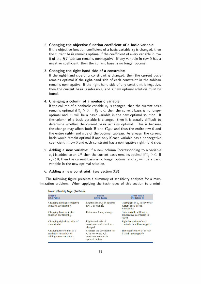
2. Changing the objective function coefficient of a basic variable:If the objective function coefficient of a basic variable xj is changed, thenthe current basis remains optimal if the coefficient of every variable in row0 of the BV tableau remains nonnegative. If any variable in row 0 has anegative coefficient, then the current basis is no longer optimal.
3. Changing the right-hand side of a constraint:If the right-hand side of a constraint is changed, then the current basisremains optimal if the right-hand side of each constraint in the tableauremains nonnegative. If the right-hand side of any constraint is negative,then the current basis is infeasible, and a new optimal solution must befound.
4. Changing a column of a nonbasic variable:If the column of a nonbasic variable xj is changed, then the current basisremains optimal if cj ≥ 0. If cj < 0, then the current basis is no longeroptimal and xj will be a basic variable in the new optimal solution. Ifthe column of a basic variable is changed, then it is usually difficult todetermine whether the current basis remains optimal. This is becausethe change may affect both B and CBV and thus the entire row 0 andthe entire right-hand side of the optimal tableau. As always, the currentbasis would remain optimal if and only if each variable has a nonnegativecoefficient in row 0 and each constraint has a nonnegative right-hand side.
5. Adding a new variable: If a new column (corresponding to a variablexj) is added to an LP, then the current basis remains optimal if cj ≥ 0. Ifcj < 0, then the current basis is no longer optimal and xj will be a basicvariable in the new optimal solution.
6. Adding a new constraint. (see Section 3.8)
The following figure presents a summary of sensitivity analyses for a max-imization problem. When applying the techniques of this section to a mini-
71

mization problem, just remember that a tableau is optimal if and only if eachvariable has a nonpositive coefficient in row 0 and the right-hand side of eachconstraint is nonnegative.
Example 3.3. Consider the following LP:
max z = 60x1 + 30x2 + 20x3s.t. 8x1 + 6x2 + x3 ≤ 48
4x1 + 2x2 + 32x3 ≤ 20
4x1 + 32x2 + 1
2x3 ≤ 8x1, x2, x3 ≥ 0
After adding slack variables s1, s2, and s3, the optimal tableau is:
Basic x1 x2 x3 s1 s2 s3 RHS
z 0 5 0 0 10 10 280
s1 0 −2 0 1 2 −8 24x3 0 −2 1 0 2 −4 8x1 1 5/4 0 0 −1/2 3/2 2
1. Suppose we change the objective function coefficient of x2 from 30 to30 + ∆. For what values of ∆ will the current set of basic variablesremain optimal ?
Solution: From the optimal tableau we know that BV = {s1, x3, x1}and NBV = {x2, s2, s3}, then
CBV =[0 20 60
], CNBV =
[30 0 0
], b =
48208
B =
1 1 80 3/2 40 1/2 2
, B−1 =
1 2 −80 2 −40 −1/2 3/2
, N =
6 0 02 1 03/2 0 1
Because x2 is a nonbasic variable, CBV has not changed. Thus, BV willremain optimal if
CNBV = CBV B−1N−CNBV
=[0 20 60
] 1 2 −80 2 −40 −1/2 3/2
6 0 02 1 03/2 0 1
− [30 + ∆ 0 0]
=[5−∆ 10 10
]≥ 0
∴ ∆ ≤ 5
72

2. Suppose we change the objective function coefficient of x1 from 60 to60 + ∆. For what values of ∆ will the current set of basic variablesremain optimal ?
Solution: The BV will remain optimal if
CNBV = CBV B−1N−CNBV
=[0 20 60 + ∆
] 1 2 −80 2 −40 −1/2 3/2
6 0 02 1 03/2 0 1
− [30 0 0]
=[5 + 5
4∆ 10− 12∆ 10 + 3
2∆]≥ 0
∴ ∆ ∈ [−4, 20]
3. Suppose we change the right-hand-side of the second constraint from 20to 20 + ∆. For what values of ∆ will the current set of basic variablesremain optimal ?
Solution: The BV will remain optimal if
b = B−1b
=
1 2 −80 2 −40 −1/2 3/2
4820 + ∆
8
=
24 + 2∆8 + 2∆2− 1
2∆
≥ 0
∴ ∆ ∈ [−4, 4]
4. Suppose we change the elements of the column for x2 from
30
62
3/2
to
43
522
. Would this change the optimal solution to the problem ?
Solution: Thus, BV will remain optimal if CNBV ≥ 0. But
CNBV = CBV B−1N−CNBV
=[0 20 60
] 1 2 −80 2 −40 −1/2 3/2
5 0 02 1 02 0 1
− [43 0 0]
=[−3 10 10
]6≥ 0
∴ The current basis is no longer optimal.
73
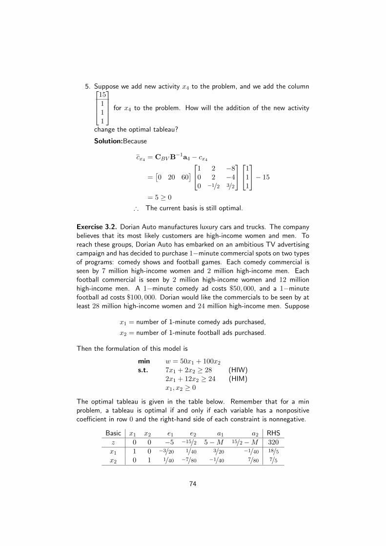
5. Suppose we add new activity x4 to the problem, and we add the column15
111
for x4 to the problem. How will the addition of the new activity
change the optimal tableau?
Solution:Because
cx4 = CBV B−1a4 − cx4
=[0 20 60
] 1 2 −80 2 −40 −1/2 3/2
111
− 15
= 5 ≥ 0
∴ The current basis is still optimal.
Exercise 3.2. Dorian Auto manufactures luxury cars and trucks. The companybelieves that its most likely customers are high-income women and men. Toreach these groups, Dorian Auto has embarked on an ambitious TV advertisingcampaign and has decided to purchase 1−minute commercial spots on two typesof programs: comedy shows and football games. Each comedy commercial isseen by 7 million high-income women and 2 million high-income men. Eachfootball commercial is seen by 2 million high-income women and 12 millionhigh-income men. A 1−minute comedy ad costs $50, 000, and a 1−minutefootball ad costs $100, 000. Dorian would like the commercials to be seen by atleast 28 million high-income women and 24 million high-income men. Suppose
x1 = number of 1-minute comedy ads purchased,
x2 = number of 1-minute football ads purchased.
Then the formulation of this model is
min w = 50x1 + 100x2s.t. 7x1 + 2x2 ≥ 28 (HIW)
2x1 + 12x2 ≥ 24 (HIM)x1, x2 ≥ 0
The optimal tableau is given in the table below. Remember that for a minproblem, a tableau is optimal if and only if each variable has a nonpositivecoefficient in row 0 and the right-hand side of each constraint is nonnegative.
Basic x1 x2 e1 e2 a1 a2 RHS
z 0 0 −5 −15/2 5−M 15/2−M 320
x1 1 0 −3/20 1/40 3/20 −1/40 18/5x2 0 1 1/40 −7/80 −1/40 7/80 7/5
74
1. Find the range of values of the cost of a comedy ad (currently $50,000)for which the current basis remains optimal.
2. Find the range of values of the number of required HIW exposures (cur-rently 28 million) for which the current basis remains optimal. If 40 millionHIW exposures were required, what would be the new optimal solution?
3. Suppose an ad on a news program costs $110,000 and reaches 12 millionHIW and 7 million HIM. Should Dorian advertise on the news program?
3.3 Finding the Dual of an LP
Associated with any LP is another LP, called the dual. Knowing the relationbetween an LP and its dual is vital to understanding advanced topics in linearand nonlinear programming. This relation is important because it gives usinteresting economic insights. Knowledge of duality will also provide additionalinsights into sensitivity analysis.
When taking the dual of a given LP, we refer to the given LP as the primal.The two problems are closely related, in the sense that the optimal solution ofone problem automatically provides the optimal solution to the other. If theprimal is a max problem, then the dual will be a min problem, and vice versa.We begin by explaining how to find the dual of a max problem in which allvariables are required to be nonnegative and all constraints are (≤) constraints(called a normal max problem). A normal max problem may be written as
max z = c1x1 + c2x2 + · · ·+ cnxns.t. a11x1 + a12x2 + · · ·+ a1nxn ≤ b1
a21x1 + a22x2 + · · ·+ a2nxn ≤ b2...am1x1 + am2x2 + · · ·+ amnxn ≤ bmx1, x2, · · · , xn ≥ 0
(3.5)
The dual of a normal max problem such as (3.5) is defined to be
min w = b1y1 + b2y2 + · · ·+ bmyms.t. a11y1 + a21y2 + · · ·+ am1ym ≥ c1
a12y1 + a22y2 + · · ·+ am2ym ≥ c2...a1ny1 + a2ny2 + · · ·+ amnym ≥ cny1, y2, · · · , ym ≥ 0
(3.6)
A min problem such as (3.6) that has all (≥) constraints and all variablesnonnegative is called a normal min problem. If the primal is a normal minproblem such as (3.6), then we define the dual of (3.6) to be (3.5).
75
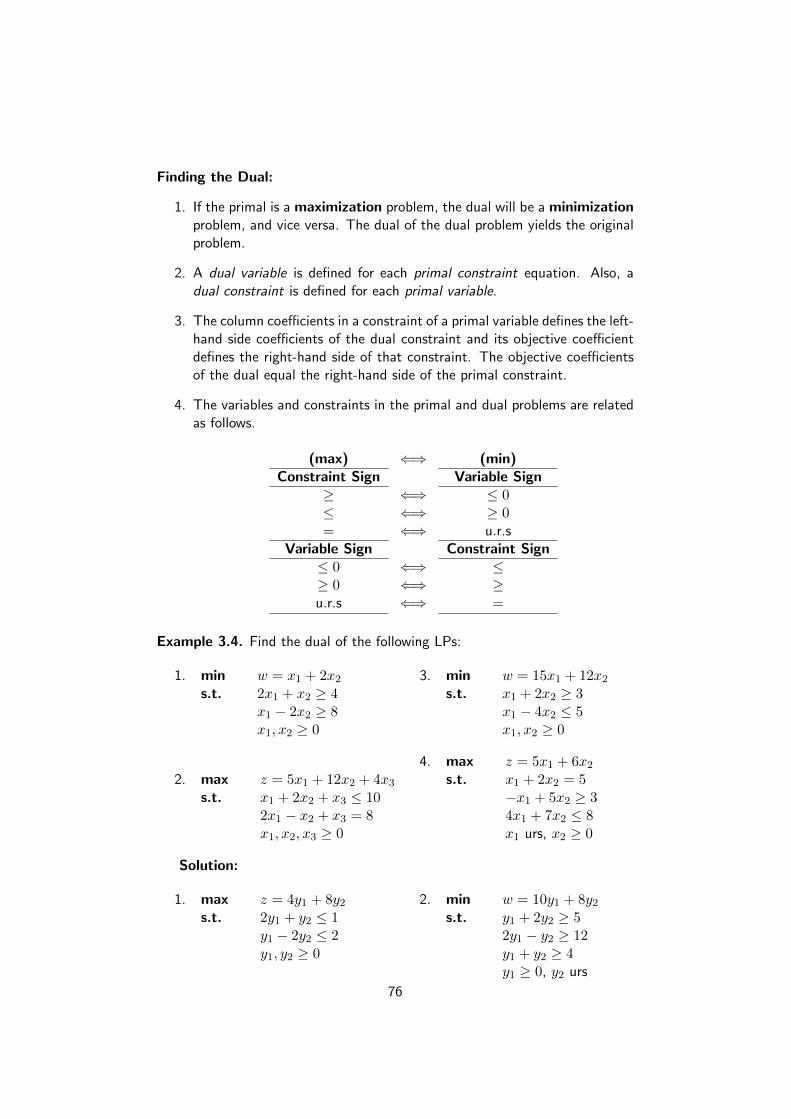
Finding the Dual:
1. If the primal is a maximization problem, the dual will be a minimizationproblem, and vice versa. The dual of the dual problem yields the originalproblem.
2. A dual variable is defined for each primal constraint equation. Also, adual constraint is defined for each primal variable.
3. The column coefficients in a constraint of a primal variable defines the left-hand side coefficients of the dual constraint and its objective coefficientdefines the right-hand side of that constraint. The objective coefficientsof the dual equal the right-hand side of the primal constraint.
4. The variables and constraints in the primal and dual problems are relatedas follows.
(max) ⇐⇒ (min)Constraint Sign Variable Sign
≥ ⇐⇒ ≤ 0≤ ⇐⇒ ≥ 0= ⇐⇒ u.r.s
Variable Sign Constraint Sign≤ 0 ⇐⇒ ≤≥ 0 ⇐⇒ ≥u.r.s ⇐⇒ =
Example 3.4. Find the dual of the following LPs:
1. min w = x1 + 2x2s.t. 2x1 + x2 ≥ 4
x1 − 2x2 ≥ 8x1, x2 ≥ 0
2. max z = 5x1 + 12x2 + 4x3s.t. x1 + 2x2 + x3 ≤ 10
2x1 − x2 + x3 = 8x1, x2, x3 ≥ 0
3. min w = 15x1 + 12x2s.t. x1 + 2x2 ≥ 3
x1 − 4x2 ≤ 5x1, x2 ≥ 0
4. max z = 5x1 + 6x2s.t. x1 + 2x2 = 5
−x1 + 5x2 ≥ 34x1 + 7x2 ≤ 8x1 urs, x2 ≥ 0
Solution:
1. max z = 4y1 + 8y2s.t. 2y1 + y2 ≤ 1
y1 − 2y2 ≤ 2y1, y2 ≥ 0
2. min w = 10y1 + 8y2s.t. y1 + 2y2 ≥ 5
2y1 − y2 ≥ 12y1 + y2 ≥ 4y1 ≥ 0, y2 urs
76

3. max z = 3y1 + 5y2s.t. y1 + y2 ≤ 15
2y1 − 4y2 ≤ 12y1 ≥, y2 ≤ 0
4. min w = 5y1 + 3y2 + 8y3s.t. y1 − y2 + 4y3 = 5
2y1 + 5y2 + 7y3 ≥ 6y1 urs, y2 ≤ 0, y3 ≥ 0
Exercise 3.3. Find the dual of the following LPs:
1. max z = 2x1 + x2s.t. −x1 + x2 ≤ 1
x1 + x2 ≤ 3x1 − 2x2 ≤ 4x1, x2 ≥ 0
2. min w = y1 − y2s.t. 2y1 + y2 ≥ 4
y1 + y2 ≥ 1y1 + 2y2 ≥ 3y1, y2 ≥ 0
3. max z = 4x1 − x2 + 2x3s.t. x1 + x2 ≤ 5
2x1 + x2 ≤ 72x2 + x3 ≥ 6x1 + x3 = 4x1 ≥ 0, x2, x3 urs
4. min w = 4y1 + 2y2 − y3s.t. y1 + 2y2 ≤ 6
y1 − y2 + 2y3 = 8y1, y2 ≥, y3 urs
3.4 The Dual Theorem and its Consequences
In this section, we discuss one of the most important results in linear program-ming: the Dual Theorem. In essence, the Dual Theorem states that the primaland dual have equal optimal objective function values (if the problems haveoptimal solutions).
If we choose any feasible solution to the max LP and any feasible solutionto the min LP (one is primal and the other is dual), the value for the min LPfeasible solution will be at least as large as the value for the max LP feasiblesolution. This result is formally stated in Lemma 3.1. Observe that the followingtwo results say nothing about which problem is primal and which is dual. Theobjective function type, max or min, that matters in this case.
Lemma 3.1. The objective values in a pair of primal-dualproblems must satisfy the following relationships:
1. For any pair of feasible primal and dual solutions,(objective valuein MAX LP
)≤
(objective valuein MIN LP
)2. At the optimum solution for both problems,(
objective valuein MAX LP
)=
(objective valuein MIN LP
)
77
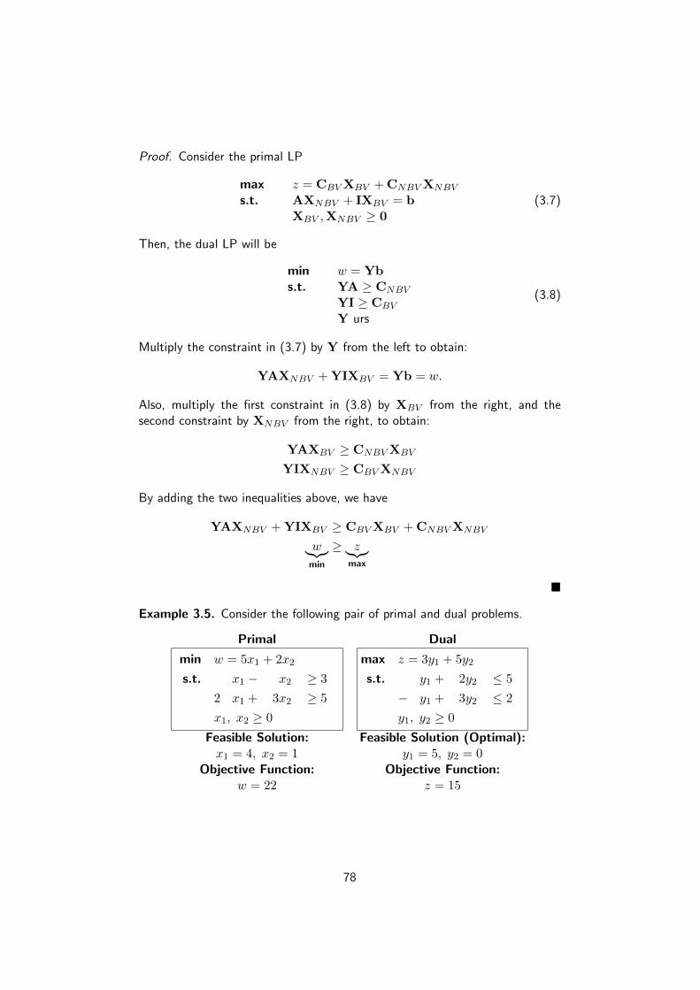
Proof. Consider the primal LP
max z = CBV XBV + CNBV XNBV
s.t. AXNBV + IXBV = bXBV ,XNBV ≥ 0
(3.7)
Then, the dual LP will be
min w = Ybs.t. YA ≥ CNBV
YI ≥ CBV
Y urs
(3.8)
Multiply the constraint in (3.7) by Y from the left to obtain:
YAXNBV + YIXBV = Yb = w.
Also, multiply the first constraint in (3.8) by XBV from the right, and thesecond constraint by XNBV from the right, to obtain:
YAXBV ≥ CNBV XBV
YIXNBV ≥ CBV XNBV
By adding the two inequalities above, we have
YAXNBV + YIXBV ≥ CBV XBV + CNBV XNBV
w︸︷︷︸min
≥ z︸︷︷︸max
�
Example 3.5. Consider the following pair of primal and dual problems.
Primal Dual
min w = 5x1 + 2x2
s.t. x1 − x2 ≥ 3
2 x1 + 3x2 ≥ 5
x1, x2 ≥ 0
max z = 3y1 + 5y2
s.t. y1 + 2y2 ≤ 5
− y1 + 3y2 ≤ 2
y1, y2 ≥ 0
Feasible Solution: Feasible Solution (Optimal):x1 = 4, x2 = 1 y1 = 5, y2 = 0
Objective Function: Objective Function:w = 22 z = 15
78
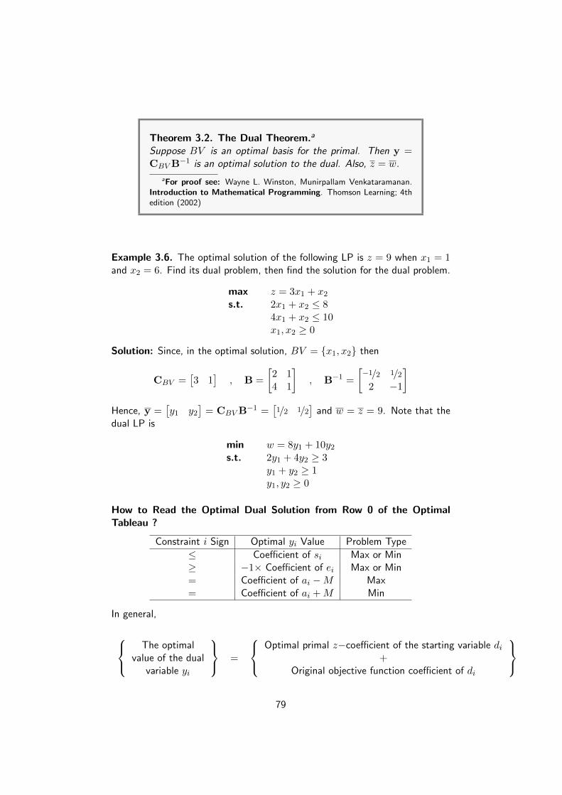
Theorem 3.2. The Dual Theorem.a
Suppose BV is an optimal basis for the primal. Then y =CBV B
−1 is an optimal solution to the dual. Also, z = w.
aFor proof see: Wayne L. Winston, Munirpallam Venkataramanan.Introduction to Mathematical Programming. Thomson Learning; 4thedition (2002)
Example 3.6. The optimal solution of the following LP is z = 9 when x1 = 1and x2 = 6. Find its dual problem, then find the solution for the dual problem.
max z = 3x1 + x2s.t. 2x1 + x2 ≤ 8
4x1 + x2 ≤ 10x1, x2 ≥ 0
Solution: Since, in the optimal solution, BV = {x1, x2} then
CBV =[3 1
], B =
[2 14 1
], B−1 =
[−1/2 1/2
2 −1
]Hence, y =
[y1 y2
]= CBV B
−1 =[1/2 1/2
]and w = z = 9. Note that the
dual LP is
min w = 8y1 + 10y2s.t. 2y1 + 4y2 ≥ 3
y1 + y2 ≥ 1y1, y2 ≥ 0
How to Read the Optimal Dual Solution from Row 0 of the OptimalTableau ?
Constraint i Sign Optimal yi Value Problem Type
≤ Coefficient of si Max or Min≥ −1× Coefficient of ei Max or Min= Coefficient of ai −M Max= Coefficient of ai + M Min
In general,
The optimal
value of the dualvariable yi
=
Optimal primal z−coefficient of the starting variable di
+Original objective function coefficient of di
79

Example 3.7. Consider the following LP.
max z = −2x1 − x2 + x3s.t. x1 + x2 + x3 ≤ 3
x2 + x3 ≥ 2x1 + x3 = 1x1, x2, x3 ≥ 0
1. Find the dual of this LP.
Solution: The dual LP is
min w = 3y1 + 2y2 + y3s.t. y1 + y3 ≥ −2
y1 + y2 ≥ −1y1 + y2 + y3 ≥ 1y1 ≥ 0, y2 ≤ 0, y3 urs
2. After adding slack variable s1, subtracting excess variable e2, and addingartificial variables a2 and a3, the Row 0 of the LP’s optimal tableau isfound to be
z + 4x1 + e2 + (M − 1)a2 + (M + 2)a3 = 0.
Find the optimal solution of the dual problem.
Solution: The starting primal variables s1, a2 and a3 uniquely correspondto the dual variables y1, y2 and y3, respectively. Thus, the optimum dualsolution is w = z = 0, and
Using the Table Using the General Formulay1 = 0
y2 = −1
y3 = (M + 2)−M = 2
y1 = 0 + 0 = 0
y2 = −M + (M − 1) = −1
y3 = −M + (M + 2) = 2
3. Suppose we change the right-hand side of the third constraint from 1 to2, what is the change on the z−value will be? Assume the current basisremains optimal.
Solution: znew = CBV B−1︸ ︷︷ ︸
y
bnew =[0 −1 2
] 322
= 2.
4. Repeat part (3) if we change the right-hand side of the second constraintfrom 2 to 5.
Solution: znew = CBV B−1︸ ︷︷ ︸
y
bnew =[0 −1 2
] 351
= −3.
80

Corollary 3.3. The primal problem is infeasible if and only ifthe normal form of the dual problem is unbounded (and viceversa).
Note 12. With regard to the primal and dual linear programming problems,exactly one of the following statements is true:
1. Both possess optimal solutions.
2. One problem has an unbounded optimal objective value, in which casethe other problem must be infeasible.
3. Both problems are infeasible.
From this note we see that duality is not completely symmetric. The best wecan say is that (here optimal means having a finite optimum, and unboundedmeans having an unbounded optimal objective value):
Primal Optimal ⇔ Dual OptimalPrimal (Dual) Unbounded ⇒ Dual (Primal) InfeasiblePrimal (Dual) Infeasible ⇒ Dual (Primal) Unbounded or InfeasiblePrimal (Dual) Infeasible ⇔ Dual (Primal) Unbounded in normal form
Note 13. The relationship between degeneracy and multiplicity of the primaland the dual optimal solutions is formulated in Theorem 3.4. Recall that de-generacy and multiplicity always refer to LP models with inequality constraints,and that degeneracy is defined for basic feasible solutions. In this theorem,the term nondegenerate in the expression “multiple and nondegenerate” meansthat there are multiple optimal solutions, and that there exists an optimal basicfeasible solution that is nondegenerate.
Theorem 3.4. Duality relationships between degeneracyand multiplicity.For any pair of primal and dual standard LP-models whereboth have optimal solutions, the following implications hold:
Primal optimal solution Dual optimal solutionMultiple ⇒ DegenerateUnique and nondeg. ⇒ Unique and nondeg.Multiple and nondeg. ⇒ Unique and degenerateUnique and degenerate ⇒ Multiple
81

Exercise 3.4.
1. Find the optimal value of the objective function for the following LP usingits dual. (Do NOT solve the dual using the simplex algorithm)
min w = 10y1 + 4y2 + 5y3
s.t. 5y1 − 7y2 + 3y3 ≥ 50
y1, y2, y3 ≥ 0
2. Consider the following LP.
max z = 2x1 + 4x2 + 4x3 − 3x4
s.t. x1 + x2 + x3 = 4
4x2 + x4 = 8
x1, x2, x3, x4 ≥ 0
(a) Write the associated dual problem.
(b) Show that the basic solution x1 and x2 is not optimal.
(c) Using x3 and x4 as starting variables, the optimal tableau is givenbelow. Determine the dual optimal solution in TWO ways, usingthe tableau.
Basic x1 x2 x3 x4 RHS
z 2 0 0 3 16
x3 3/4 0 1 −1/4 2x2 1/4 1 0 1/4 2
3. For the following LP,
max z = −x1 + 5x2
s.t. x1 + 2x2 ≤ 0.5
−x1 + 3x2 ≤ 0.5
x1, x2 ≥ 0
row 0 of the optimal tableau is z + 0.4s1 + 1.4s2 = ? . Determine theoptimal z−value for the given LP.
4. Consider the following linear programming problem:
max z = 4x1 + x2
s.t. 3x1 + 2x2 ≤ 6
6x1 + 3x2 ≤ 10
x1, x2 ≥ 0
Suppose that in solving this problem, row 0 of the optimal tableau is
found to be z + 2x2 + s2 =20
3. Use the Dual Theorem to prove that the
computations must be incorrect.
82

5. Solve the dual of the following problem, and then find its optimal solu-tion from the solution of the dual. Does the solution of the dual offercomputational advantages over solving the primal directly?
min w = 50x1 + 60x2 + 30x3
s.t. 5 x1 + 5x2 + 3 x3 ≥ 50
x1 + x2 − x3 ≥ 20
7 x1 + 6x2 − 9 x3 ≥ 30
5 x1 + 5x2 + 5 x3 ≥ 35
2 x1 + 4x2 − 15x3 ≥ 10
12x1 + 10x2 ≥ 90
x2 − 10x3 ≥ 20
x1, x2, x3 ≥ 0
6. Consider the following LP:
max z = 5x1 + 2x2 + 3x3
s.t. x1 + 5x2 + 2x3 = 15
x1 − 5x2 − 6x3 ≤ 20
x1, x2, x3 ≥ 0
Given that the artificial variable a1 and the slack variable s2 form thestarting basic variables and that M was set equal to 100 when solving theproblem, the optimal tableau is given as:
Basic x1 x2 x3 a1 s2 RHS
z 0 23 7 105 0 75
x1 1 5 2 1 0 15s2 0 −10 −8 −1 1 5
Write the associated dual problem, and determine its optimal solution intwo ways.
83

3.5 Shadow Prices
It is often important for managers to determine how a change in a constraint’sright-hand side changes the LP’s optimal z−value.
Definition 3.2. The shadow price of the ith constraint is theamount by which the optimal value of the objective function isimproved (improved means increased in max LP and decreasedin min LP) if we increase bi (the RHS of that constraint) by1 (from bi to bi + 1).
Note 14.
1. The previous definition assumes that after the RHS of constraint i hasbeen changed to bi + 1, the current basis remains optimal.
2. The shadow price of the ith constraint of a max LP is the optimal valueof the ith dual variable yi. Also, the shadow price of the ith constraintof a min LP is −1× the optimal value of the ith dual variable yi
znew = Yb =[y1 · · · yi · · · ym
]
b1...
bi + 1...bm
= y1b1 + · · ·+ yi (bi + 1) + · · ·+ ymbm
= (y1b1 + · · ·+ yibi + · · ·+ ymbm) + yi
= zold + yi
∴ znew − zold = yi
3. In max LP, the shadow price for a (≤) constraint is nonnegative, for a(≥) is nonpositive, and for (=) is urs. Also, in min LP, the shadow pricefor a (≤) constraint is nonpositive, for a (≥) is nonnegative, and for (=)is urs.
4. In general, if the RHS of the ith constraint is increased by an amount∆bi, then
znew = zold + (∆bi) yi if the LP is max
znew = zold − (∆bi) yi if the LP is min
84
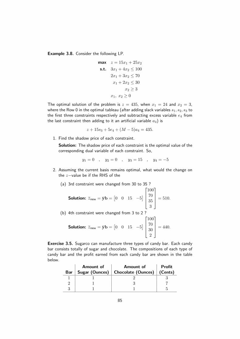
Example 3.8. Consider the following LP.
max z = 15x1 + 25x2
s.t. 3x1 + 4x2 ≤ 100
2x1 + 3x2 ≤ 70
x1 + 2x2 ≤ 30
x2 ≥ 3
x1, x2 ≥ 0
The optimal solution of the problem is z = 435, when x1 = 24 and x2 = 3,where the Row 0 in the optimal tableau (after adding slack variables s1, s2, s3 tothe first three constraints respectively and subtracting excess variable e4 fromthe last constraint then adding to it an artificial variable a4) is
z + 15s3 + 5e4 + (M − 5)a4 = 435.
1. Find the shadow price of each constraint.
Solution: The shadow price of each constraint is the optimal value of thecorresponding dual variable of each constraint. So,
y1 = 0 , y2 = 0 , y3 = 15 , y4 = −5
2. Assuming the current basis remains optimal, what would the change onthe z−value be if the RHS of the
(a) 3rd constraint were changed from 30 to 35 ?
Solution: znew = yb =[0 0 15 −5
] 10070353
= 510.
(b) 4th constraint were changed from 3 to 2 ?
Solution: znew = yb =[0 0 15 −5
] 10070302
= 440.
Exercise 3.5. Sugarco can manufacture three types of candy bar. Each candybar consists totally of sugar and chocolate. The compositions of each type ofcandy bar and the profit earned from each candy bar are shown in the tablebelow.
Amount of Amount of ProfitBar Sugar (Ounces) Chocolate (Ounces) (Cents)
1 1 2 32 1 3 73 1 1 5
85

Fifty oz of sugar and 100 oz of chocolate are available. After defining xi tobe the number of Type i candy bars manufactured, Sugarco should solve thefollowing LP:
max z = 3x1 + 7x2 + 5x3
s.t. x1 + x2 + x3 ≤ 50
2x1 + 3x2 + x3 ≤ 100
x1, x2, x3 ≥ 0
After adding slack variables s1 and s2, the optimal tableau is as shown in thetable below.
Basic x1 x2 x3 s1 s2 RHS
z 3 0 0 4 1 300
x3 1/2 0 1 3/2 −1/2 25x2 1/2 1 0 −1/2 1/2 25
Using this optimal tableau, answer the following questions:
1. Find the shadow prices for the Sugarco problem.
2. If 60 oz of sugar were available, what would be Sugarco’s profit?
3.6 Duality and Sensitivity Analysis
From the dual theorem we demonstrate the following: Assuming that a set ofbasic variables BV is feasible, then BV is optimal if and only if the associateddual solution CBV B
−1 is dual feasible.
Unbounded =⇒ infeasible, then feasible =⇒ bounded
This result can be used for an alternative way of doing the following types ofsensitivity analysis:
1. Changing the objective function coefficient of a nonbasic variable.
2. Changing a column of a nonbasic variable.
3. Adding a new variable.
Since primal optimality and dual feasibility are equivalent, the above changes willleave the current basic optimal if and only if the current dual solution CBV B
−1
remains dual feasible.
Example 3.9. Consider the following LP.
max z = 60x1 + 30x2 + 20x3
s.t. 8x1 + 6x2 + x3 ≤ 48
86

4x1 + 2x2 +3
2x3 ≤ 20
2x1 +3
2x2 +
1
2x3 ≤ 8
x1, x2, x3 ≥ 0
The dual of the problem is:
min w = 48y1 + 20y2 + 8y3
s.t. 8y1 + 4y2 + 2 y3 ≥ 60
6y1 + 2y2 +3
2y3 ≥ 30
y1 +3
2y2 +
1
2y3 ≥ 20
y1, y2, y3 ≥ 0
The optimal solution for the primal was z = 280, s1 = 24, x3 = 8, x1 = 2︸ ︷︷ ︸Basic
,
x2 = s2 = s3 = 0︸ ︷︷ ︸NonBasic
. Also, the optimal dual solution (constraint shadow prices)
are y1 = 0, y2 = 10, y3 = 10.
1. Let c2 be the coefficient of x2 in the objective function. For what valuesof c2 will the current basis remain optimal?
Solution: If y1 = 0, y2 = 10, y3 = 10 remains dual feasible, then thecurrent basis and the values of all the variables are unchanged. Note thatif the objective function coefficient for x2 is changed, then the first andthird dual constraints remain unchanged, but the second dual constraint
is changed to 6y1 + 2y2 +3
2y3 ≥ c2. Thus, the current basis remains
optimal if c2 satisfies 6(0) + 2(10) +3
2(10) ≥ c2, or c2 ≤ 35.
2. Suppose we change the elements of the column for x2 from
30
62
3/2
to
43
522
, does the current basis remain optimal?
Solution: Changing the column for the nonbasic variable leaves the firstand third dual constraints unchanged but changes the second to
5y1 + 2y2 + 2y3 ≥ 43
87
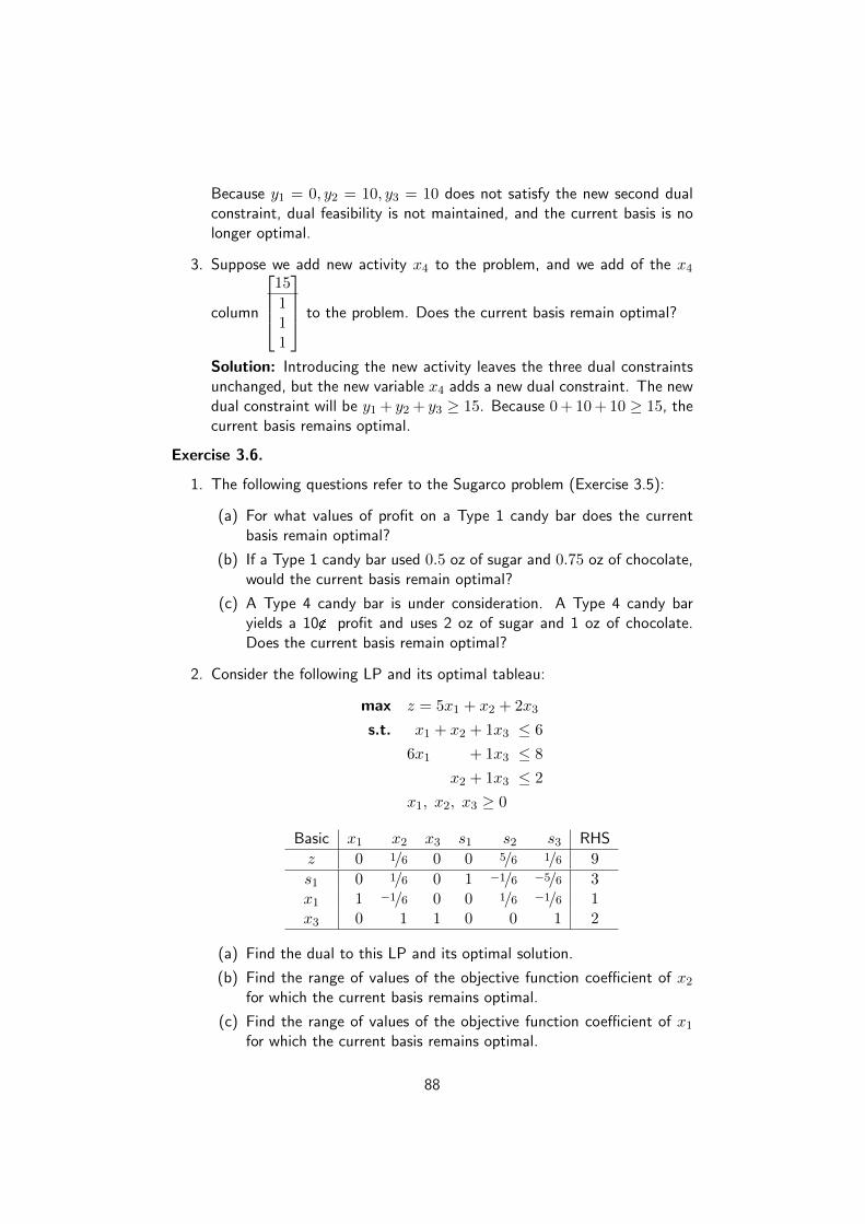
Because y1 = 0, y2 = 10, y3 = 10 does not satisfy the new second dualconstraint, dual feasibility is not maintained, and the current basis is nolonger optimal.
3. Suppose we add new activity x4 to the problem, and we add of the x4
column
15
111
to the problem. Does the current basis remain optimal?
Solution: Introducing the new activity leaves the three dual constraintsunchanged, but the new variable x4 adds a new dual constraint. The newdual constraint will be y1 + y2 + y3 ≥ 15. Because 0 + 10 + 10 ≥ 15, thecurrent basis remains optimal.
Exercise 3.6.
1. The following questions refer to the Sugarco problem (Exercise 3.5):
(a) For what values of profit on a Type 1 candy bar does the currentbasis remain optimal?
(b) If a Type 1 candy bar used 0.5 oz of sugar and 0.75 oz of chocolate,would the current basis remain optimal?
(c) A Type 4 candy bar is under consideration. A Type 4 candy baryields a 10� profit and uses 2 oz of sugar and 1 oz of chocolate.Does the current basis remain optimal?
2. Consider the following LP and its optimal tableau:
max z = 5x1 + x2 + 2x3
s.t. x1 + x2 + 1x3 ≤ 6
6x1 + 1x3 ≤ 8
x2 + 1x3 ≤ 2
x1, x2, x3 ≥ 0
Basic x1 x2 x3 s1 s2 s3 RHS
z 0 1/6 0 0 5/6 1/6 9
s1 0 1/6 0 1 −1/6 −5/6 3x1 1 −1/6 0 0 1/6 −1/6 1x3 0 1 1 0 0 1 2
(a) Find the dual to this LP and its optimal solution.
(b) Find the range of values of the objective function coefficient of x2for which the current basis remains optimal.
(c) Find the range of values of the objective function coefficient of x1for which the current basis remains optimal.
88

3.7 Complementary Slackness
The Theorem of Complementary Slackness is an important result that relatesthe optimal primal and dual solutions. To state this theorem, we assume thatthe primal is a normal max problem with variables x1, x2, · · · , xn and m of (≤)constraints. Then the dual is a normal min problem with variables y1, y2, · · · , ymand n of (≥) constraints.
max z = c1x1 + · · ·+ cnxn
s.t. a11 x1 + · · ·+ a1nxn ≤ b1
a21 x1 + · · ·+ a2nxn ≤ b2...
......
am1x1 + · · ·+ amnxn ≤ bm
xi ≥ 0, ∀i = 1, 2, · · · , n
min w = b1y1 + · · ·+ bmym
s.t. a11y1 + · · ·+ am1ym ≥ c1
a12y1 + · · ·+ am2ym ≥ c2...
......
a1ny1 + · · ·+ amnym ≥ cn
yj ≥ 0, ∀j = 1, 2, · · · ,m
Let s1, s2, · · · , sm be the slack variables for the primal, and e1, e2, · · · , enbe the excess variables for the dual.
max z = c1x1 + · · ·+ cnxn
s.t. a11 x1 + · · ·+ a1nxn + s1 = b1
a21 x1 + · · ·+ a2nxn + s2 = b2...
......
am1x1 + · · ·+ amnxn + sm = bm
xi ≥ 0, ∀i = 1, 2, · · · , nsj ≥ 0, ∀j = 1, 2, · · · ,m
min w = b1y1 + · · ·+ bmym
s.t. a11y1 + · · ·+ am1ym − e1 = c1
a12y1 + · · ·+ am2ym − e2 = c2...
......
a1ny1 + · · ·+ amnym − en = cn
yj ≥ 0, ∀j = 1, 2, · · · ,mei ≥ 0, ∀i = 1, 2, · · · , n
Theorem 3.5. Let x =
x1...xn
be a feasible primal solution
and y =[y1 · · · ym
]be a feasible dual solution. Then x is
primal optimal and y is dual optimal, (z = w), if and only if
xiei = 0 , ∀i = 1, 2, · · · , nyjsj = 0 , ∀j = 1, 2, · · · ,m
89

In other words, if a constraint in either the primal or dual isnon binding (sj > 0 or ei > 0), then the corresponding (com-plementary) variable in the other problem must equal 0.
Proof. Multiply each constraint in the primal in standard form by its corre-sponding (complementary) dual variable:
a11x1y1 + · · ·+ a1n xny1 + s1y1 = b1y1
a21x1y2 + · · ·+ a2n xny2 + s2y2 = b2y2...
......
am1x1ym + · · ·+ amnxnym + smym = bmym
Add all the constraints above together:
(a11x1y1 + · · ·+ a1nxny1 + · · ·+am1x1ym + · · ·+ amnxnym)
+ (s1y1 + · · ·+ smym)
= b1y1 + · · ·+ bmym
= w
(3.9)
Now, multiply each constraint in the dual in standard form by its corresponding(complementary) primal variable:
a11y1x1 + · · ·+ am1 ymx1 − e1x1 = c1x1
a12y1x2 + · · ·+ am2 ymx2 − e2x2 = c2x2...
......
a1ny1xn + · · ·+ amnymxn − enxn = cnxn
Add all the constraints above together:
(a11y1x1 + · · ·+ am1ymx1 + · · ·+a1ny1xn + · · ·+ amnymxn)
− (e1x1 + · · ·+ enxn)
= c1x1 + · · ·+ cnxn
= z
(3.10)
Subtract equation (3.10) from equation (3.9) to obtain:
s1y1 + s2y2 + · · ·+ smym + e1x1 + e2x2 + · · ·+ enxn = w − z (3.11)
If x is primal optimal and y is dual optimal, then z = w, and then
s1y1 + s2y2 + · · ·+ smym + e1x1 + e2x2 + · · ·+ enxn = 0
90

Since, all x’s, y’s, s’s, and e’s are all nonnegative, then
xiei = 0 , ∀i = 1, 2, · · · , nyjsj = 0 , ∀j = 1, 2, · · · ,m
Also, if
xiei = 0 , ∀i = 1, 2, · · · , nyjsj = 0 , ∀j = 1, 2, · · · ,m
then 0 = z − w and hence z = w. So, x is primal optimal and y is dualoptimal. �
Example 3.10. Consider the following LP.
max z = 5x1 + 3x2 + x3
s.t. 2x1 + x2 + x3 ≤ 6
x1 + 2x2 + x3 ≤ 7
x1, x2, x3 ≥ 0
The optimal solution to the problem is z =49
3, x1 =
5
3, x2 =
8
3, and x3 =
s1 = s2 = 0. Use complementary slackness theorem to find the optimal dualsolution of the problem.Solution: The dual LP is
min w = 6y1 + 7y2
s.t. 2y1 + y2 ≥ 5
y1 + 2y2 ≥ 3
y1 + y2 ≥ 1
y1, y2 ≥ 0
Because x1 > 0 and x2 > 0 then the optimal dual solution must have e1 = 0and e2 = 0. This means that for the optimal dual solution, the first and secondconstraints must be binding. So we know that the optimal values of y1 andy2 may be found by solving the first and second dual constraints as equalities.Thus, the optimal values of y1 and y2 must satisfy
2y1 + y2 = 5
y1 + 2y2 = 3
Solving these equations simultaneously shows that the optimal dual solution
must have y1 =7
3and y2 =
1
3, with w = z =
49
3.
91

Exercise 3.7. Consider the following LP.
max z = 3x1 + 4x2 + x3 + 5x4
s.t. x1 + 2x2 + x3 + 2x4 ≤ 5
2x1 + 3x2 + x3 + 3x4 ≤ 8
x1, x2, x3, x4 ≥ 0
The optimal solution to the problem is z = 13, x1 = 1, x2 = x3 = 0, andx4 = 2. Use complementary slackness theorem to find the optimal dual solutionof the problem.
3.8 The Dual−Simplex Method
In the simplex algorithm presented in Chapter 2 the problem starts at a (basic)feasible solution. Successive iterations continue to be feasible until the optimalis reached at the last iteration. The algorithm is sometimes referred to as theprimal simplex method.
This section presents two additional algorithms: The dual simplex and thegeneralized simplex.
� In the dual simplex, the LP starts at a better than optimal infeasible(basic) solution. Successive iterations remain infeasible and (better than)optimal until feasibility is restored at the last iteration.
� The generalized simplex combines both the primal and dual simplex meth-ods in one algorithm. It deals with problems that start both non-optimaland infeasible. In this algorithm, successive iterations are associated withbasic feasible or infeasible (basic) solutions. At the final iteration, thesolution becomes optimal and feasible (assuming that one exists).
Dual Simplex Algorithm: The crux of the dual simplex method is to startwith a better than optimal and infeasible basic solution. The optimality andfeasibility conditions are designed to preserve the optimality of the basic solutionswhile moving the solution iterations toward feasibility.
� To start the LP optimal and infeasible, two requirements must be met:
– The objective function must satisfy the optimality condition of theregular simplex method.
– All the constraints must be of the type (≤), regardless the type ofproblem either max or min. This condition requires converting any(≥) to (≤) simply by multiplying both sides of the inequality (≥)by −1. If the LP includes (=) constraints, the equation can bereplaced by two inequalities. For example, x1 +x2 = 1 is equivalent
to
{x1 + x2 ≤ 1
x1 + x2 ≥ 1or
{x1 + x2 ≤ 1
−x1 − x2 ≤ −1
92

� After converting all the constraints to (≤), the starting solution is infea-sible if at least one of the right-hand sides of the inequalities is strictlynegative.
� Dual feasibility condition. The leaving variable, xr is the basic variablehaving the most negative value (ties are broken arbitrarily). If all the basicvariables are nonnegative, the algorithm ends.
� Dual optimality condition. Given that xr is the leaving variable, letcj be the reduced cost of nonbasic variable xj and arj the constraintcoefficient in the xr−row and xj−column of the tableau. The enteringvariable is the nonbasic variable with arj < 0 that corresponds to
minNonBasic xj
{∣∣∣∣ cjarj∣∣∣∣ , arj < 0
}Note that
1. Ties are broken arbitrarily.
2. If arj ≥ 0 for all nonbasic xj , the problem has no feasible solution.
Example 3.11. Use the dual−simplex algorithm for solving the following LPproblem.
min w = 5x1 + 6x2
s.t. x1 + x2 ≥ 2
4x1 − x2 ≥ 4
x1, x2 ≥ 0
Solution: After converting all the constraints to (≤), then adding slack variabless1 and s2 to the constraints, the LP in standard form is
min w − 5x1 − 6x2 = 0
s.t. − x1 − x2 + s1 = −2
−4x1 + x2 + s2 = −4
x1, x2, s1, s2 ≥ 0
The initial tableau and all following tableaus, using the dual-simplex algorithm,are shown below.
↓Iteration [0] Basic x1 x2 s1 s2 RHS Optimal
w −5 −6 0 0 0 but nots1 −1 −1 1 0 −2 feasible
← s2 −4 1 0 1 −4
93

↓Iteration [1] Basic x1 x2 s1 s2 RHS Optimal
w 0 −29/4 0 −5/4 5 but not← s1 0 −5/4 1 −1/4 −1 feasible
x1 1 −1/4 0 −1/4 1
Iteration [2] Basic x1 x2 s1 s2 RHS Optimalw 0 −1 −5 0 10 ands2 0 5 −4 1 4 feasiblex1 1 1 −1 0 2
Example 3.12. Use the dual−simplex algorithm for solving the following LPproblem.
max z = −4x1 − 2x2
s.t. x1 + x2 = 1
− 3x1 + x2 ≥ 2
x1, x2 ≥ 0
Solution: After converting all the constraints to (≤), then adding slack variabless1, s2 and s3 to the constraints, the LP in standard form is
max z + 4x1 + 2x2 = 0
s.t. x1 + x2 + s1 = 1
− x1 − x2 + s2 = −1
3x1 − x2 + s3 = −2
x1, x2, s1, s2, s3 ≥ 0
The initial tableau and all following tableaus, using the dual-simplex algorithm,are shown below.
↓Iteration [0] Basic x1 x2 s1 s2 s3 RHS Optimal
z 4 2 0 0 0 0 but nots1 1 1 1 0 0 1 feasibles2 −1 −1 0 1 0 −1
← s3 3 −1 0 0 1 −2
Iteration [1] Basic x1 x2 s1 s2 s3 RHS Since s1 leavesz 10 0 0 0 2 −4 with no entering
← s1 4 0 1 0 1 −1 variable, then thes2 −4 0 0 1 −1 1 solution is infeasiblex2 −3 1 0 0 −1 2
94

Note 15. The dual simplex method is often used to find the new optimalsolution to an LP after a constraint is added. When a constraint is added, oneof the following three cases will occur:
1. The current optimal solution satisfies the new constraint.
2. The current optimal solution does not satisfy the new constraint, but theLP still has a feasible solution.
3. The additional constraint causes the LP to have no feasible solutions.
Example 3.13. Consider the following LP and its optimal tableau.
max z = 6x1 + x2
s.t. x1 + x2 ≤ 5
2 x1 + x2 ≤ 6
x1, x2 ≥ 0
Basic x1 x2 s1 s2 RHS
z 0 2 0 3 18
s1 0 1/2 1 −1/2 2x1 1 1/2 0 1/2 3
Find the optimal solution to this LP if we add the constraint
1. 3x1 + x2 ≤ 10.
Solution: After converting the constraint to (=) by adding s3 to theconstraint, we obtain:
Basic x1 x2 s1 s2 s3 RHS
z 0 2 0 3 0 18
s1 0 1/2 1 −1/2 0 2x1 1 1/2 0 1/2 0 3
s3 3 1 0 0 1 10
Basic x1 x2 s1 s2 s3 RHS The solutionz 0 2 0 3 0 18 is optimals1 0 1/2 1 −1/2 0 2 and feasiblex1 1 1/2 0 1/2 0 3s3 0 −1/2 0 −3/2 1 1
2. x1 − 2x2 ≥ 6.
Solution: After converting the constraint to (≤) then adding s3 to theconstraint, we obtain:
Basic x1 x2 s1 s2 s3 RHS
z 0 2 0 3 0 18
s1 0 1/2 1 −1/2 0 2x1 1 1/2 0 1/2 0 3
s3 −1 2 0 0 1 −6
95

Basic x1 x2 s1 s2 s3 RHS Since s3 leavesz 0 2 0 3 0 18 with no enterings1 0 1/2 1 −1/2 0 2 variable, then thex1 1 1/2 0 1/2 0 3 solution is infeasibles3 0 5/2 0 1/2 1 −3
3. 8x1 + x2 ≤ 12.
Solution: After converting the constraint to (=) by adding s3 to theconstraint, we obtain:
Iteration [0] Basic x1 x2 s1 s2 s3 RHSz 0 2 0 3 0 18s1 0 1/2 1 −1/2 0 2x1 1 1/2 0 1/2 0 3
s3 8 1 0 0 1 12
↓Iteration [0] Basic x1 x2 s1 s2 s3 RHS The solution
z 0 2 0 3 0 18 is optimals1 0 1/2 1 −1/2 0 2 but infeasiblex1 1 1/2 0 1/2 0 3
← s3 0 −3 0 −4 1 −12
Iteration [1] Basic x1 x2 s1 s2 s3 RHS The solutionz 0 0 0 1/3 2/3 10 is optimals1 0 0 1 −7/3 1/6 0 and feasiblex1 1 0 0 −1/6 1/6 1x2 0 1 0 4/3 −1/3 4
Generalized Simplex Algorithm: The (primal) simplex algorithm starts fea-sible but not optimal. The dual simplex starts (better than) optimal but infeasi-ble. What if an LP model starts both not optimal and infeasible? The followingexample illustrates what we call the generalized simplex algorithm for solvingLP problems with this situation.
Example 3.14. Consider the following LP.
max z = x1 − 3x2
s.t. x1 − x2 ≤ 2
x1 + x2 ≥ 4
2x1 + 2x2 ≥ 3
x1, x2 ≥ 0
96

The model can be put in the following tableau form in which the starting basicsolution (s1, s2, s3) is both non-optimal (because x1 has a negative reducedcost) and infeasible (because s2 = −4, s3 = −3).
↓Iteration [0] Basic x1 x2 s1 s2 s3 RHS The solution
z −1 3 0 0 0 0 is not optimals1 1 −1 1 0 0 2 and infeasible
← s2 −1 −1 0 1 0 −4s3 −2 −2 0 0 1 −3
Remove infeasibility first by applying a version of the dual simplex feasibilitycondition that selects s2 as the leaving variable. To determine the enteringvariable, all we need is a nonbasic variable whose constraint coefficient in thes2−row is strictly negative. The selection can be done without regard to opti-mality, because it is nonexistent at this point anyway. In the present example,x1 and x2 have negative coefficient in the s2−row and x1 is selected as theentering variable. The result is the following tableau:
↓Iteration [1] Basic x1 x2 s1 s2 s3 RHS The solution
z 0 4 0 −1 0 4 is not optimal← s1 0 −2 1 1 0 −2 and infeasible
x1 1 1 0 −1 0 4s3 0 0 0 −2 1 5
At this point, s1 leaves the solution and x2 have negative coefficient in thes1−row and is selected as the entering variable. The result is the followingtableau:
Iteration [2] Basic x1 x2 s1 s2 s3 RHS The solutionz 0 0 2 1 0 0 is optimalx2 0 1 −1/2 −1/2 0 1 and feasiblex1 1 0 1/2 −1/2 0 3s3 0 0 0 −2 1 5
The solution in the preceding tableau is now feasible and fortunately optimal.
Dual Simplex with Artificial Constraints: In example (3.14), the dual sim-plex is not applicable directly, because x1 does not satisfy the maximizationoptimality condition. Show that by adding the artificial constraint x1 ≤ M(where M is sufficiently large not to eliminate any feasible points in the originalsolution space), and then using the new constraint as a pivot row, the selectionof x1 as the entering variable (because it has the most negative objective coeffi-cient) will render an all-optimal objective row. Next, carry out the regular dualsimplex method on the modified problem. All the iterations are shown below.
97
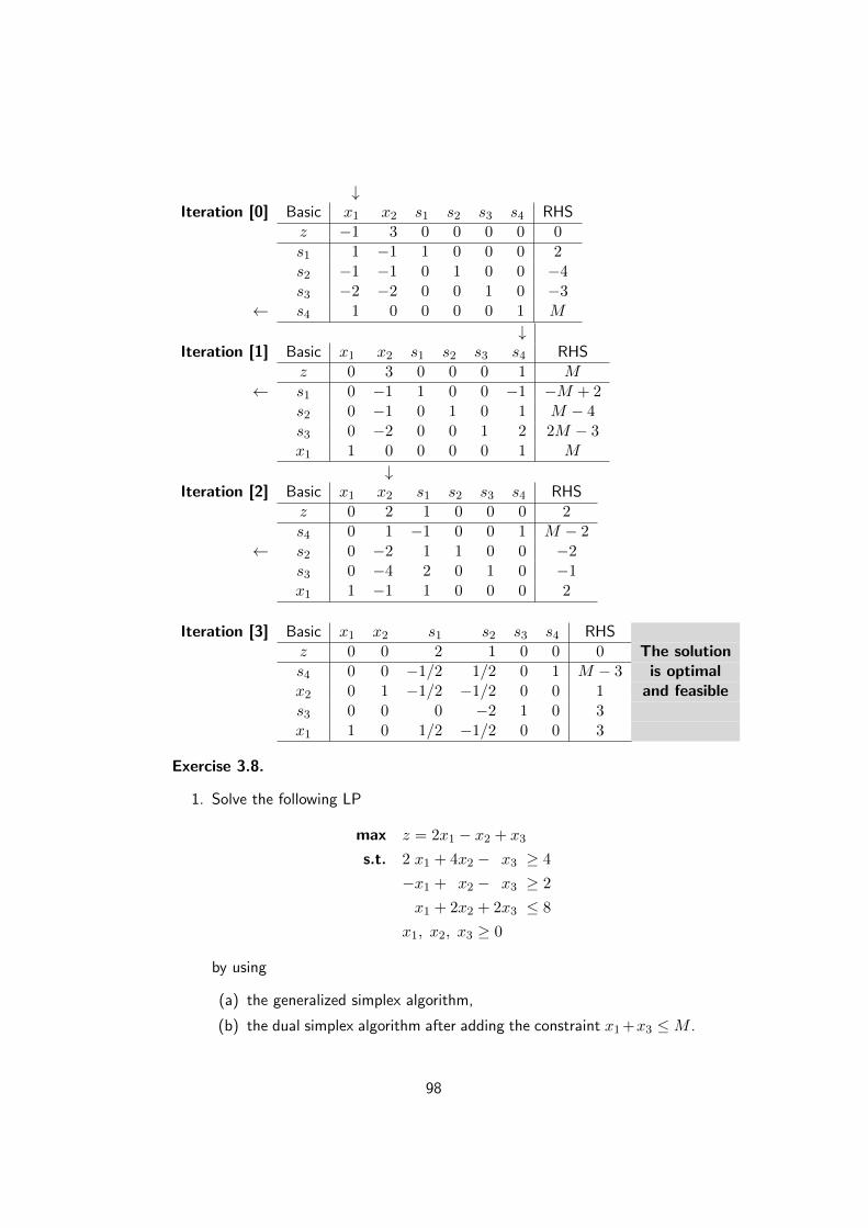
↓Iteration [0] Basic x1 x2 s1 s2 s3 s4 RHS
z −1 3 0 0 0 0 0s1 1 −1 1 0 0 0 2s2 −1 −1 0 1 0 0 −4s3 −2 −2 0 0 1 0 −3
← s4 1 0 0 0 0 1 M
↓Iteration [1] Basic x1 x2 s1 s2 s3 s4 RHS
z 0 3 0 0 0 1 M← s1 0 −1 1 0 0 −1 −M + 2
s2 0 −1 0 1 0 1 M − 4s3 0 −2 0 0 1 2 2M − 3x1 1 0 0 0 0 1 M
↓Iteration [2] Basic x1 x2 s1 s2 s3 s4 RHS
z 0 2 1 0 0 0 2s4 0 1 −1 0 0 1 M − 2
← s2 0 −2 1 1 0 0 −2s3 0 −4 2 0 1 0 −1x1 1 −1 1 0 0 0 2
Iteration [3] Basic x1 x2 s1 s2 s3 s4 RHSz 0 0 2 1 0 0 0 The solutions4 0 0 −1/2 1/2 0 1 M − 3 is optimalx2 0 1 −1/2 −1/2 0 0 1 and feasibles3 0 0 0 −2 1 0 3x1 1 0 1/2 −1/2 0 0 3
Exercise 3.8.
1. Solve the following LP
max z = 2x1 − x2 + x3
s.t. 2 x1 + 4x2 − x3 ≥ 4
−x1 + x2 − x3 ≥ 2
x1 + 2x2 + 2x3 ≤ 8
x1, x2, x3 ≥ 0
by using
(a) the generalized simplex algorithm,
(b) the dual simplex algorithm after adding the constraint x1+x3 ≤M .
98

2. Use the dual simplex method to solve the following LP:
max z = −2x1 − x3
s.t. x1 + x2 − x3 ≥ 5
x1 − 2x2 + 4x3 ≥ 8
x1, x2, x3 ≥ 0
3. Solve the following LP in three different ways. Which method appears tobe the most efficient computationally?
min w = 6x1 + 7x2 + 3x3 + 5x4
s.t. 5x1 + 6x2 − 3x3 + 4x4 ≥ 12
x2 − 5x3 − 6x4 ≥ 10
2x1 + 5x2 + x3 + x4 ≥ 8
x1, x2, x3, x4 ≥ 0
4. Instead of solving a problem using all of its constraints, we can start byidentifying the so called secondary constraints. These are the constraintsthat we suspect are least restrictive in terms of the optimum solution.The model is solved using the remaining (primary) constraints. We maythen add the secondary constraints one at a time. A secondary constraintis discarded if it satisfies the available optimum. The process is repeateduntil all the secondary constraints are accounted for. Apply the proposedprocedure to the following LP:
max z = 5x1 + 6x2 + 3x3
s.t. 5 x1 + 5x2 + 3x3 ≤ 50
x1 + x2 − x3 ≤ 20
7 x1 + 6x2 − 9x3 ≤ 30
5 x1 + 5x2 + 5x3 ≤ 35
12x1 + 6x2 ≤ 90
x2 − 9x3 ≤ 20
x1, x2, x3 ≥ 0[Hint: Start with the first, third, and fourth constraint. The associated
solution is x1 = 0, x2 = 6.2, x3 = 0.8. This solution automaticallysatisfies the second, fifth, and sixth constraint. Hence, these conditionsare discarded as redundant and the optimal solution for the problem is
x1 = 0, x2 = 6.2, x3 = 0.8, z = 39.6.]
99

Answers
DON’T EVEN DARE PEEK AT THE SOLUTIONS TO AN EXERCISE UNTILYOU’VE GENUINELY TRIED TO SOLVE THE EXERCISE !!
Chapter 1 Exercise 1.1
1. Let x1 = number of desks produced per day, x2 = number of chairsproduced per day. Then, the formulation of the problem is
max z = 50x1 + 100x2
s.t.1
200x1 +
1
80x2 ≤ 1
1
150x1 +
1
110x2 ≤ 1
x1 ≤ 120x2 ≤ 60x1 ≥ 0, x2 ≥ 0
2. Let x1 = number of Type 1 Trucks produced daily, x2 = number of Type2 Trucks produced daily. Then, the formulation of the problem is
max z = 300x1 + 500x2
s.t.1
800x1 +
1
700x2 ≤ 1
1
500x1 +
1
200x2 ≤ 1
x1 ≥ 0, x2 ≥ 0
3. Let x1 = number of hours spent working, x2 = number of hours spentplaying. Then, the formulation of the problem is
max z = x1 + 5x2s.t. x1 − 3x2 ≥ 0
x1 + x2 ≤ 8x1 ≥ 0, x2 ≥ 0
4. Let x1 = number of hours of Process 1, x2 = number of hours of Process2. Then, the formulation of the problem is
min w = 4x1 + x2s.t. 3x1 + x2 ≥ 10
x1 + x2 ≥ 5x1 ≥ 3x1 ≥ 0, x2 ≥ 0
100

5. Let x1 = number of units of A, x2 = number of units of B. Then, theformulation of the problem is
max z = 20x1 + 50x2
s.t.x1
x1 + x2≥ 0.80
x1 ≤ 1002x1 + 4x2 ≤ 240x1 ≥ 0, x2 ≥ 0
6. Let x1 = number of rectangular tables, x2 = number of round tables.Then, the formulation of the problem is
min w = 28x1 + 52x2s.t. 6x1 + 10x2 ≥ 250
x1 + x2 ≤ 35x1 ≤ 15x1 ≥ 0, x2 ≥ 0
7. Let x1 = number of units of food F1 to be eaten, x2 = number of unitsof food F2 to be eaten. Then, the formulation of the problem is
min w = 0.05x1 + 0.03x2s.t. 2x1 + x2 ≥ 400
x1 + 2x2 ≥ 5004x1 + 4x2 ≥ 1400x1 ≥ 0, x2 ≥ 0
8. Let x1 = number of appliances shipped to terminal A, x2 = number ofappliances shipped to terminal A. Then, the formulation of the problemis
min w = 12x1 + 16x2s.t. x1 + x2 ≤ 1200
x1 ≥ 400x2 ≥ 500x1 ≥ 0, x2 ≥ 0
9. Let x1 = pounds of food A purchased, x2 = pounds of food B purchased.Then, the formulation of the problem is
min w = 1.3x1 + 0.8x2s.t. 5x1 + 2x2 ≥ 60
3x1 + 2x2 ≥ 454x1 + x2 ≥ 30x1 ≥ 0, x2 ≥ 0
101

Chapter 1 Exercise 1.2
1.
2. Hyperplane: (a), (e). Half-Space: (b). Neither: (c), (d), (f)
3. Convex: (A), (B), (F), (H)
4. (a)(1 + t, 3 + t, 2− 3t
); 0 ≤ t ≤ 1
(b)(1 + t, 3 + t, 2− 3t
)=(1.5, 3.5, 0.5
)if t = 0.5 ∈
[0, 1]
Chapter 1 Exercise 1.3
1. (a) IV (b) II (c) I (d) III
2. If there are > and or < constraints, then a problem may have no optimalsolution. Consider the problem max z = x subject to x < 1. Clearly, thisproblem has no optimal solution (there is no largest number smaller than1!!)
3. (a) 16 (b) 55 (c) 84 (d) 90
4. (a) 32 (b) 55 (c) 36 (d) 32
102

5. (a) 2a < b
(b)a
3< b < 2a
(c) b <a
3(d) b = 2a
(e) b =a
3
6. (a) south-east (down-right)
(b) south-west (down-left)
(c) north-west (up-left)
7. (a) north-west (up-left) (b) south-east (down-right)
8. The constraints x + y ≤ 6 and x + y ≤ 4 are redundant.
9. The redundant constraint is y ≤ 3
−x + y ≤ 1
x + y ≤ 5
x− 2y ≤ 2
y ≤ 3
x ≥ 1
x, y ≥ 0
10.
103

11. No feasible region
12. x1 = 2, x2 = 3 by solving the two constraint-equations.
13. (a) w = 12, x1 = 3, x2 = 0
(b) unbounded optimal solution
(c) w = 6, x1 = 0, x2 = 6
(d) z = 4, x1 = 0, x2 = 6
(e) z = 16, x1 = 6, x2 = 2
(f) w = 14, x1 = 3, x2 = 2
Chapter 2 Exercise 2.1
1. max z = 2x1 + 3x2 + 5y3 + 5y4s.t. −x1 − x2 + y3 + y4 + s1 = 5
−6x1 + 7x2 − 9y3 − 9y4 + s2 = 4x1 + x2 + 4y3 + 4y4 = 10x1, x2, y3, y4, s1, s2 ≥ 0
2. 22x1 − 4x2 ≥ −7⇒ 22x1 − 4x2 − e1 = −7⇒ −22x1 + 4x2 + e1 = 7
22x1 − 4x2 ≥ −7⇒ −22x1 + 4x2 ≤ 7⇒ −22x1 + 4x2 + s1 = 7
3. x y1 y2−6 0 610 10 00 0 6
Chapter 2 Exercise 2.2
1. (a) max z = 2x1 + 3x2s.t. x1 + 3x2 + s1 = 12
3x1 + 2x2 + s2 = 12x1, x2, s1, s2 ≥ 0
104
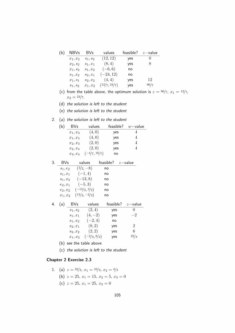
(b) NBVs BVs values feasible? z−value
x1, x2 s1, s2 (12, 12) yes 0x2, s2 s1, x1 (8, 4) yes 8x1, s2 s1, x2 (−6, 6) nos1, x2 s2, x1 (−24, 12) nox1, s1 s2, x2 (4, 4) yes 12s1, s2 x1, x2 (12/7, 24/7) yes 96/7
(c) from the table above, the optimum solution is z = 96/7, x1 = 12/7,x2 = 24/7.
(d) the solution is left to the student
(e) the solution is left to the student
2. (a) the solution is left to the student
(b) BVs values feasible? w−value
x1, x3 (4, 0) yes 4x1, x4 (4, 0) yes 4x2, x3 (2, 0) yes 4x2, x4 (2, 0) yes 4x3, x4 (−4/7, 16/7) no
3. BVs values feasible? z−value
s1, e2 (3/2,−8) nos1, x1 (−1, 4) nos1, x2 (−13, 8) noe2, x1 (−5, 3) noe2, x2 (−13/2, 3/2) nox1, x2 (13/3,−2/3) no
4. (a) BVs values feasible? z−value
s1, s2 (2, 4) yes 0s1, x1 (4,−2) yes −2s1, x2 (−2, 4) nos2, x1 (8, 2) yes 2s2, x2 (2, 2) yes 6x1, x2 (−2/3, 8/3) yes 22/3
(b) see the table above
(c) the solution is left to the student
Chapter 2 Exercise 2.3
1. (a) z = 32/3, x1 = 10/3, x2 = 4/3
(b) z = 25, x1 = 15, x2 = 5, x3 = 0
(c) z = 25, x1 = 25, x2 = 0
105

(d) z = 12, x1 = 4, x2 = 4, x3 = 4
2. BVs values feasible? z−value
x1 30 yes 150x2 10 yes −60x3 6 yes 18x4 5 yes −25x5 10 yes 120s1 30 yes 0
Chapter 2 Exercise 2.4
1. w = −5, x1 = 0, x2 = 5
2. w = −2, x1 = 0, x2 = 2
3. w = −7.5, x1 = 0, x2 = 1.5
4. w = −9, x1 = 3, x2 = 0
5. w = −48, x1 = 0, x2 = 4, x3 = 0, x4 = 8
Chapter 2 Exercise 2.5
1. (a) w = 1, x1 = 0, x2 = 0, x3 = 1
(b) w = 2, x1 = 2, x2 = 0, x3 = 0
(c) w = 4, x1 = 2, x2 = 0
(d) z = 5, x1 = 1, x2 = 2
2. w = 214/7, x1 = 66/7, x2 = 8/7, x3 = 0, x4 = 0
3. z = 10, x1 = 4, x2 = 0, x3 = 2
Chapter 2 Exercise 2.6
1. (a) iterations 2 and 3 are degenerate, and degeneracy is removed initeration 4.
(b) the solution is left to the student
(c) 3 iterations
2. z = 4, x1 = 4, x2 = 0, x3 = 0
3. z = 10 when: x1 = 0, x2 = 0, x3 = 10/3
x1 = 0, x2 = 5, x3 = 0
x1 = 1, x2 = 4, x3 = 1/3
106
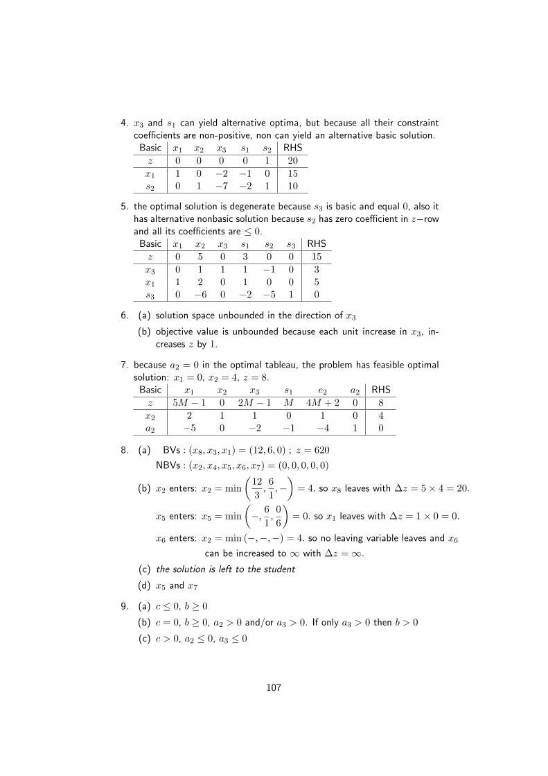
4. x3 and s1 can yield alternative optima, but because all their constraintcoefficients are non-positive, non can yield an alternative basic solution.
Basic x1 x2 x3 s1 s2 RHS
z 0 0 0 0 1 20
x1 1 0 −2 −1 0 15s2 0 1 −7 −2 1 10
5. the optimal solution is degenerate because s3 is basic and equal 0, also ithas alternative nonbasic solution because s2 has zero coefficient in z−rowand all its coefficients are ≤ 0.
Basic x1 x2 x3 s1 s2 s3 RHS
z 0 5 0 3 0 0 15
x3 0 1 1 1 −1 0 3x1 1 2 0 1 0 0 5s3 0 −6 0 −2 −5 1 0
6. (a) solution space unbounded in the direction of x3
(b) objective value is unbounded because each unit increase in x3, in-creases z by 1.
7. because a2 = 0 in the optimal tableau, the problem has feasible optimalsolution: x1 = 0, x2 = 4, z = 8.
Basic x1 x2 x3 s1 e2 a2 RHS
z 5M − 1 0 2M − 1 M 4M + 2 0 8
x2 2 1 1 0 1 0 4a2 −5 0 −2 −1 −4 1 0
8. (a) BVs : (x8, x3, x1) = (12, 6, 0) ; z = 620
NBVs : (x2, x4, x5, x6, x7) = (0, 0, 0, 0, 0)
(b) x2 enters: x2 = min
(12
3,6
1,−)
= 4. so x8 leaves with ∆z = 5× 4 = 20.
x5 enters: x5 = min
(−, 6
1,0
6
)= 0. so x1 leaves with ∆z = 1× 0 = 0.
x6 enters: x2 = min (−,−,−) = 4. so no leaving variable leaves and x6
can be increased to ∞ with ∆z =∞.
(c) the solution is left to the student
(d) x5 and x7
9. (a) c ≤ 0, b ≥ 0
(b) c = 0, b ≥ 0, a2 > 0 and/or a3 > 0. If only a3 > 0 then b > 0
(c) c > 0, a2 ≤ 0, a3 ≤ 0
107
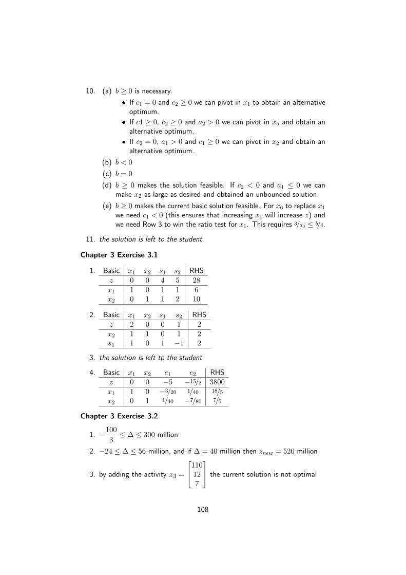
10. (a) b ≥ 0 is necessary.
� If c1 = 0 and c2 ≥ 0 we can pivot in x1 to obtain an alternativeoptimum.
� If c1 ≥ 0, c2 ≥ 0 and a2 > 0 we can pivot in x5 and obtain analternative optimum.
� If c2 = 0, a1 > 0 and c1 ≥ 0 we can pivot in x2 and obtain analternative optimum.
(b) b < 0
(c) b = 0
(d) b ≥ 0 makes the solution feasible. If c2 < 0 and a1 ≤ 0 we canmake x2 as large as desired and obtained an unbounded solution.
(e) b ≥ 0 makes the current basic solution feasible. For x6 to replace x1we need c1 < 0 (this ensures that increasing x1 will increase z) andwe need Row 3 to win the ratio test for x1. This requires 3/a3 ≤ b/4.
11. the solution is left to the student
Chapter 3 Exercise 3.1
1. Basic x1 x2 s1 s2 RHS
z 0 0 4 5 28
x1 1 0 1 1 6x2 0 1 1 2 10
2. Basic x1 x2 s1 s2 RHS
z 2 0 0 1 2
x2 1 1 0 1 2s1 1 0 1 −1 2
3. the solution is left to the student
4. Basic x1 x2 e1 e2 RHS
z 0 0 −5 −15/2 3800
x1 1 0 −3/20 1/40 18/5x2 0 1 1/40 −7/80 7/5
Chapter 3 Exercise 3.2
1. −100
3≤ ∆ ≤ 300 million
2. −24 ≤ ∆ ≤ 56 million, and if ∆ = 40 million then znew = 520 million
3. by adding the activity x3 =
110127
the current solution is not optimal
108

Chapter 3 Exercise 3.3
1. min w = y1 + 3y2 + 4y3s.t. −y1 + y2 + y3 ≥ 2
y1 + y2 − 2y3 ≥ 1y1, y2, y3 ≥ 0
2. max z = 4x1 + x2 + 3x3s.t. 2x1 + x2 + x3 ≤ 1
x1 + x2 + x3 ≤ −1x1, x2, x3 ≥ 0
3. min w = 5y1 + 7y2 + 6y3 + 4y4s.t. y1 + 2y2 + y4 ≥ 4
y1 + y2 + 2y3 = −1y3 + y4 = 2y1, y2 ≥ 0, y3 ≤ 0, x4 urs
4. max z = 6x1 + 8x2s.t. x1 + x2 ≤ 4
2x1 − x2 ≤ 22x2 = −1x1 ≤, x2 urs
Chapter 3 Exercise 3.4
1. w = 250/3.
2. (a) the solution is left to the student
(b) CNBV = CBV B−1N−CNBV =
[−2 7/2
](c) � y = CBV B
−1 =[4 0
]=[y1 y2
]� Using the general formula: y1 = 0 + 4 = 4
y2 = 3 + (−3) = 0
3. z = CBV B−1︸ ︷︷ ︸
y
b =[0.4 1.4
] [0.50.5
]= 0.9
4. since y =[0 1
]then w = 10 6= 20/3
5. x1 = 0, x2 = 20, x3 = 0, z = 1200
6. the solution is left to the student
Chapter 3 Exercise 3.5
1. y1 = 4, y2 = 1
2. znew = zold + 10× 4 = 340
Chapter 3 Exercise 3.6
1. (a) dual constraint for x1 is y1 + 2y2 ≥ c1. since y1 = 4 and y2 = 1 thecurrent basis is still optimal if c1 ≤ 6
(b) dual constraint for Type 1 Candy Bar is nowy12
+3y24≥ 3. since
y1 = 4 and y2 = 1 does not satisfy this constraint, the current basisis no longer optimal
109
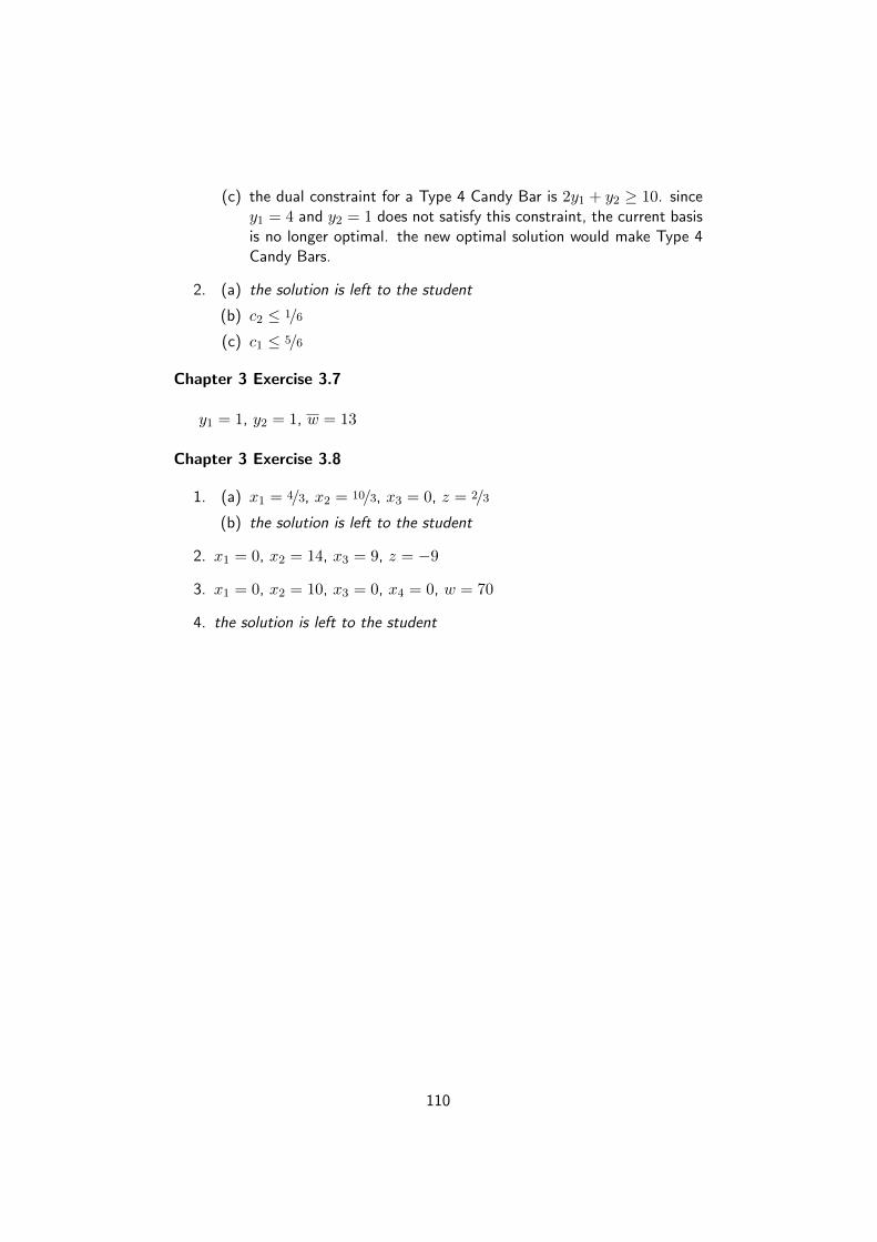
(c) the dual constraint for a Type 4 Candy Bar is 2y1 + y2 ≥ 10. sincey1 = 4 and y2 = 1 does not satisfy this constraint, the current basisis no longer optimal. the new optimal solution would make Type 4Candy Bars.
2. (a) the solution is left to the student
(b) c2 ≤ 1/6
(c) c1 ≤ 5/6
Chapter 3 Exercise 3.7
y1 = 1, y2 = 1, w = 13
Chapter 3 Exercise 3.8
1. (a) x1 = 4/3, x2 = 10/3, x3 = 0, z = 2/3
(b) the solution is left to the student
2. x1 = 0, x2 = 14, x3 = 9, z = −9
3. x1 = 0, x2 = 10, x3 = 0, x4 = 0, w = 70
4. the solution is left to the student
110