linear programming applied to dairy cattle selection
TRANSCRIPT

Retrospective Theses and Dissertations Iowa State University Capstones, Theses andDissertations
1992
Linear programming applied to dairy cattleselectionBevin Lyal HarrisIowa State University
Follow this and additional works at: https://lib.dr.iastate.edu/rtd
Part of the Agriculture Commons, and the Genetics Commons
This Dissertation is brought to you for free and open access by the Iowa State University Capstones, Theses and Dissertations at Iowa State UniversityDigital Repository. It has been accepted for inclusion in Retrospective Theses and Dissertations by an authorized administrator of Iowa State UniversityDigital Repository. For more information, please contact [email protected].
Recommended CitationHarris, Bevin Lyal, "Linear programming applied to dairy cattle selection " (1992). Retrospective Theses and Dissertations. 9997.https://lib.dr.iastate.edu/rtd/9997

INFORMATION TO USERS
This manuscript has been reproduced from the microfilm master. UMI
films the text directly from the original or copy submitted. Thus, some
thesis and dissertation copies are in typewriter face, while others may
be from any type of computer printer.
The quality of this reproduction is dependent upon the quality of the
copy submitted. Broken or indistinct print, colored or poor quality
illustrations and photographs, print bleedthrough, substandard margins,
and improper aligimient can adversely affect reproduction.
In the unlikely event that the author did not send UMI a complete
manuscript and there are missing pages, these will be noted. Also, if
unauthorized copyright material had to be removed, a note will indicate
the deletion.
Oversize materials (e.g., maps, drawings, charts) are reproduced by
sectioning the original, beginning at the upper left-hand corner and
continuing from left to right in equal sections with small overlaps. Each
original is also photographed in one exposure and is included in
reduced form at the back of the book.
Photographs included in the original manuscript have been reproduced xerographically in this copy. Higher quality 6" x 9" black and white
photographic prints are available for any photographs or illustrations
appearing in this copy for an additional charge. Contact UMI directly to order.
University Microfilms International A Bell & Howell Information Company
300 Nortfi Zeeb Road, Ann Arbor, IVII48106-1346 USA 313/761-4700 800/521-0600

Order Number 9234812
Linear programming applied to dairy cattle selection
Harris, Bevin Lyal, Ph.D.
Iowa State University, 1992
U M I 300N.ZeebRd. Ann Arbor, MI 48106

Linear programming applied to dairy cattle selection
by
Bevin Lyal Harris
A Dissertation Submitted to the
Graduate Faculty in Partial Fulfillment of the
Requirements for the Degree of
DOCTOR OF PHILOSOPHY
Department: Animal Science
Major: Animal Breeding
Approved:
In Charge of Major Work
For the Major Department
For the Gradume CqMe$e
Iowa State University
Ames, Iowa
1992
Signature was redacted for privacy.
Signature was redacted for privacy.
Signature was redacted for privacy.

ii
TABLE OF CONTENTS
GENERAL INTRODUCTION 1
Explanation of Dissertation Format 2
PART I. LINEAR PROGRAMMING—A REVIEW 3
Introduction 4
Definition of a linear programming problem 4
Geometric solution to the linear programming problem 5
Simplex method for solving linear programs 8
Obtaining an initial basic feasible solution 11
Phase I 11
Phase II 12
An illustration of the simplex method 14
Duality 16
Further computational considerations 19
References 21
PART II. THE ECONOMIC VALUE OF RESPONSE TO SELECTION FROM DAIRY
SIRE SELECTION 22
INTRODUCTION 23
LITERATURE REVIEW 24
Response to selection 24
Calculation of genetic gain from multistage selection 26
An example of multistage selection index 29
Economic weights for selection index 31
Parameter estimates for production and non-productiontraits for Holstein dairy cattle 37
Introduction 37
Production and somatic cell count 37
Fertility 42
Linear type and liveweight 44
PAPER 1. PREDICTION OF RESPONSE WITH OVERLAPPING GENERATIONS ACCOUNTING
FOR MULTISTAGE SELECTION 48
Summary 48
Introduction 48
Prediction of response with overlapping generations 49
iii
Response to selection with overlapping generations accounting for
multistage selection 52
Asymptotic response to selection 55
Application: Modelling genetic gain from dairy progeny testing scheme 58
Appendix 63
PAPER 2. ECONOMIC VALUE OF RESPONSE FROM SIRE SELECTION IN DAIRY CATTLE—
A LINEAR PROGRAMMING MODEL 65
Abstract • 65
Introduction 65
Literature Reveiw 66
Methods 68
Linear programming model 68
Response to selection constraints 68
Herd nutrition and liveweight constraints 72
Milk production, mastitis, and somatic cell score constraints 74
Salvage value and calf value constraints 75
Cash flow constraints 75
Objective Function 76
Derivation of the economic value of response to selection 76
Results and discussion 77
Conclusions 81
Appendix 82
REFERENCES 86
PART III. APPLICATION OF LINEAR PROGRAMMING TO LONGEVITY IN
DAIRY CATTLE 94
LITERATURE REVIEW 95
Introduction 96
Genetics of longevity 96
Relationships between longevity and milk production 98
Relationships between longevity and type 101
Indirect evaluation of longevity 104
Conclusions 106
PAPER 3. ANALYSIS OF HERDLIFE IN GUERNSEY DAIRY CATTLE 107
Abstract 107
Introduction 107

iv
Materials and methods 108
Herdlife data 108
Herdlife and milk production 110
Herdlife and linear type data 110
Prediction of 48-mo herdlife from linear type data 111
Results and discussion 112
Conclusions 117
Acknowledgements 119
PAPER 4. OPTIMIZATION OF LINEAR TYPE TRAITS FOR HERDLIFE 120
Abstract 120
Introduction 120
Materials and methods 121
Results and discussion 125
Holstein 72 mo herdlife 125
Guernsey 48 mo herdlife 129
Conclusions 131
Acknowledgements 132
REFERENCES 133
GENERAL SUMMARY 137
APPENDIX 1. DETAILED ACCOUNT OF DAIRY FARM LINEAR
PROGRAMMING MODEL 140
Response to selection constraints 140
Metabolizable energy, protein requirements, and live weight constraints 141
Metabolizable energy 141
Protein Requirements 142
Metabolic liveweight 143
Young stock rearing requirements 145
Formulation of metabolizable energy, protein requirements, and
liveweight constraints 146
Milk production, somatic cell score and mastitis constraints 148
Salvage value and calf value constraints 150
Cashflow constraints 151
Objective function 152
Numerical Example of the dairy herd constraints 152

V
References 156
APPENDIX 2. LINEAR PROGRAMMING MODEL PARAMETERS 157
APPENDIX 3. GENEFLOW FORTRAN 77 PROGRAM l6l
Notes l6l
Program listing l6l
Example Input 181
Example output 183
APPENDIX 4. MATHEMATICA PROGRAM FOR COMPUTING LINEAR CONSTRAINTS
FROM BIVARIATE NORMAL CONTOURS 184
Example Output 188

vi
Figure 1
PAPER 1
Figure 1.
Figure 2.
PAPER 2
Figure 1.
Figure Al.
PAPER 3
Figure 1.
Figure 2.
PAPER 4
Figure 1.
Figure 2.
LIST OF FIGURES
PART I
The boundaries of the half-planes defined by the inequality constraints in the
diet problem example. The solid lines represent the boundry of the feasible
region. The dashed lines represent the part of each constraint which is
outside the feasible region, xl = kg of bread, x2 = kg of meat, and x3 = kg
of vegetables 6
PART II
Response to a single cycle of selection for protein yield 6l
Response to cumulative selection for protein yield 6l
Constraints computed from the 75% bivariate normal density
for the relationship between the rates of genetic gain for milkfat
and milk protein and a density plot of the observations for
response to selection per year from the gene-flow simulation 73
Bivariate normal contour with four tangent linear constraints 84
PART III
Scatter plot of true herdlife predicted transmitting abilities,
PTAs, for 124 Guernsey sires computed from multiple trait
mixed model and linear type trait predicted transmitting abilities 117
Scatter plot of functional herdlife predicted transmitting abilities,
PTAs, for 124 Guernsey sires computed from multiple trait mixed
model and linear type trait predicted transmitting abilities 118
The bounding constraints for foot angle and rear legs side view
(genetic correlation .34) used in the Holstein linear programming
models and transmitting abilities for 617 Holstein sires 124
The bounding constraints for stature and strength (genetic
correlation .74) used in the Guernsey linear programming
models and transmitting abilities for 124 Guernsey sires 125

vil
Figure 3. The loss in optimal 72 month true (THL) and functional herdlife
(FHL) resulting from changing transmitting abilities for
individual linear type traits from their minimum (left) to
maximum value (right) and to a value of zero ( #) in grade
Holstein cattle
Figure 4. Relationship between udder depth and true and functional
herdlife transmitting abilities in grade Holstein cattle
Figure 5. The loss in optimal 72 month true (THL) and functional herdlife
(FHL) resulting from changing transmitting abilities for
individual linear type traits from their minimum (left) to
maximum value (right) and to a value of zero (•) in registered
Guernsey cattle
Figure 6. Relationship between udder depth and true and functional
herdlife transmitting abilities in registered Guernsey cattle
127
128
130
131

viii
LIST OF TABLES
PART I
Table 1. Food composition and costs for the diet problem
PART 11
LITERATURE REVIEW
Table 1. Means, number of records, standard deviations, SD, and
heritabilities, h^, for first parity milk, fat and protein yield
Table 2. Genetic and phenotypic correlations between individual
production traits for first parity
Table 3. Repeatability estimates for milk production from Welper (1991)
Table 4. Means, number of records, standard deviations, SD, and
heritabilities, h^, for somatic cell count
Table 5. Genetic and phenotypic correlations between production traits
and somatic cell score surveyed from the literature
Table 6. Means, number of records, standard deviations, SD, and
heritabilities, h^, for days open
Table 7. Repeatability estimates for days open
Table 8. Genetic and phenotypic correlations between production
and days open
Table 9. Means, number of records, standard deviations, SD, and
heritabilities, h^, for linear type
Table 10. Genetic and phenotypic correlations between linear type traits
Table 11. Means, number of records, standard deviations, SD,
and heritabilities, h~, for liveweight
Table 12. Genetic and phenotypic correlations between production
and liveweight
PAPER 1
Table 1. Population parameters.
Table 2. Proportion of animals used as breeders in the four
reproductive pathways for the numerical example of a progeny
testing scheme
5
38
39
40
40
41
42
43
43
45
46
46
47
57
58

ix
Table 3.
Table 4.
Table 5.
PAPER 2
Table 1.
Table 2.
Table 3.
Table 4.
Table 5
Table 6.
Table 7.
LITERATURE
Table 1
Table 2
PAPER 3
Table 1.
Means, genetic standard deviations (SD) and heritabilities (h^)
genetic correlations , phenotypic correlations, repeatabilities (R)
and economic weights (EW) for milk, fat and protein yield (kg) 59
Genetic gain (kg) for the three traits and the asymptotic
response to selection calculated using Eq. 24 60
Response to a single cycle of selection for the three production traits for
model 1 and model 2 (all amounts in kg) 62
Genetic correlations (above diagonal), phenotypic correlations
(below diagonal) and heritabilities used in the geneflow
simulation (on diagonal)
Maximum, minimum, mean, and standard deviation (SD) for the
response to selection per year from the gene-flow simulation
The correlations between response to selection per year from
the gene-flow simulation
Price, cost, and interest rate parameters representative of
Iowa, USA from 1970 to 1989
Optimal rates of genetic gain for four planning horizons
Relative economic value of a unit standard deviation genetic
gain for production and non-production traits under four
planning horizions
Coefficients for use in economic sire selection index
PART III
REVIEW
Genetic and phenotypic correlations among stayability and
milk and fat yield from the literature
Genetic correlations among herdlife and linear type traits
from the literature
Unadjusted means and standard deviations, heritability
estimates with approximate standard errors 1 sire variance
estimates (a^), and error variance estimates (o^) for herdlife traits
70
71
71
78
79
81
82
100
103
113

113
114
114
115
116
122
126
129
157
158
159
160
160
X
Genetic (above diagonal) and phenotypic correlations between
Guernsey herdlife traits
Phenotypic and genetic correlations between Guernsey herdlife
and production traits
Phenotypic and genetic correlations between Guernsey type
and herdlife traits for registered Guernsey cows
Weights for predicting true and functional herdlife from
Guernsey linear type and 95% lower bound confidence
intervals, CI, for the weights
Direct and indirect predicted transmitting abilities, PTA, for
true and functional herdlife for 5 randomly choosen sires
Weights to predict transmitting abilities for true and functional
herdlife from transmitting abilities for linear traits in grade
holstein and registered Guernsey cattle
Optimal transmitting abilities for linear traits for predicting
true and functional herdlife transmitting abilities in grade
holstein cattle
Optimal transmitting abilities for linear traits for predicting
true and functional herdlife transmitting abilities in registered
Guernsey cattle
Geneflow parameters for milk, fat, protein yield, and liveweight and
somatic cell score
Herdlife parameters for milk, fat, protein yield, and liveweight,
salvage value and calf value
Days open parameters for milk, fat, and protein yield
Liveweight gain parameters for salvage value
Feed characteristics for the linear programming model

xi
DEDICATION
This thesis is dedicated to my parents, Lyal and Nilla Harris and my wife. Erica whose
encouragement and support made this endeavor possible.

xii
ACKNOWLEGDEMENTS
I would like to thank my advisor Dr. A. E. Freeman for his support, guidance and friendship.
I would also like to acknowledge the following: the members of my committee Drs R. L. Willham,
G. W. Ladd, L. C. Christian, D. A. Harville and the late V. A. Sposito; the research team at the
Livestock Improvement Corporation, Hamilton, New Zealand, in particular Dr. B. W. Wickham,
Dr. P. Shannon, and R. G. Jackson; the staff and graduate students in the Animal Breeding
Department; lastly Drs A. L. Rae, H. T. Blair and R. D. Anderson of Massey University, New
Zealand. All have given assistance, friendship and encouragement either at Iowa State University
or in the planning of my Ph.D study.
Financial support for this study was provided in part by the Livestock Improvement
Corporation, New Zealand and a William Geogetti sholarship.
This dissertation was produced electronically using Aldus PageMaker® on an Apple®
Macintosh® computer. Mathematical equations were typeset using Design Science's MathType®.
Illustrations and graphs were created in Mathematica® and enhanced with Aldus Freehand®.
Text was set in ITC® Garamond and Helevetica. Mathematical text was set in Times and Belmont.
1
GENERAL INTRODUCTION
Application of modelling to livestock production research has increased over recent years.
Modelling enables the estimation of parameters that can not be estimated by other methods.
Models are an important tool in the understanding of livestock production systems, since they
provide a way of representing existing knowledge, the components of the system and their
interactions, and the inputs and outputs. Specific models fall into two categories, statistical and
economic. The economic model category contains areas: cost benefit analysis, decision analysis,
linear and dynamic programming, Markov decision analysis and system simulation. Linear
programming is a technique for determining the optimal allocation of resources to competing
activities. Linear programming has been used extensively in agriculture for farm planning
resource allocation and least cost diet formulation. The objective of this dissertation is apply
linear programming to two areas within dairy cattle breeding, namely, determination of
economic weights for selection indices and optimization herd life using linear type traits.
Linear programming procedures are reviewed in Part I of the dissertation. The simplex
method for solving linear programming problems is discussed in detail. Also covered are
concepts of duality and computational aspects of solving large scale linear programs.
Linear programming methods are used to determine the economic value of response to
selection at the farm level in Part IL A method for predicting response to selection with multiple
stage selection and overlapping generations is outlined. This method is used to compute rates
of response to selection for nine traits from a dairy cattle progeny testing scheme. The responses
to selection per year are inputs to the farm level linear programming model. The objective of
the linear programing model is to maximize the accrued net income over a predetermined
planning horizon. The linear programming model is used to determine the optimal rates of
response to selection for four planning horizons. Further, relative economic weights for nine
traits for each planning horizon are computed utilizing the results from the linear programming
model. The use of linear a programming model allows the animals within the system and
management of the farm system to be optimized simultaneously, optimization ensures resources
available to the system are efficiently used, and the effect of response to selection over a number
of years can modelled.
In Part III linear programming methods are applied to modelling herd life in Holstein and
Guernsey dairy cattle. Genetic and phenotypic (co)variances between herd life and linear type
traits in Guernsey cattle are computed. The genetic covariances are used to estimate weights
for indirect prediction of herd life transmitting abilities from linear type transmitting abilities. The
weights and the genetic covariances among individual linear type traits are used to build a linear
programming model. The objective of the linear programming model is compute the values for
the linear type trait transmitting abilities that maximize herd life for both registered Guernsey
2
and grade Holsteins. Further, the linear programming models are used to determine the effect
of individual type traits on herd life.
Explanation of Dissertation Format
The dissertation is divided into four parts. Part I is a review of linear programming pertinent
to Parts II, III and Appendix 1. Part's II and III each contains an introduction, literature reviews
and two papers that report the authors work. Each of the papers in Parts II and III is intended
for publication.The references for the papers and the literature reviews are combined at the end
of each part.
The first paper in Part II has been published in Theoretical and Applied Genetics. Paper 2
in Part II has different organization because it is written for publication in a different scientific
journal. Papers 3 and 4 in Part III have the same organization that differs from the organization
of papers 1 and 2 in Part II because they are written for publication in a third scientific journal.
The following list gives the publication details for each paper:
1. Prediction of response with overlapping generations accounting for multiple stage
selection. Published in Theoretical and Applied Genetics (1991) 82:329.
2. Economic value of response to selection from sire selection in dairy cattle—A linear
programming model. Submitted for publication in Agricultural Systems.
3. Analysis of herd life in Guernsey Dairy Cattle. Accepted for publication in the Journal
of Dairy Science.
4. Optimization of linear type traits for herd life. Submitted for publication in the Journal
of Dairy Science.

3
PART I. LINEAR PROGRAMMING—A REVIEW

4
Introduction
Linear programming was primarily developed by George B. Dantzig in 1947 as a technique
for studying the diversified activities of the U. S. Air Force (Dorfman et al., 1958). Dantzig
developed the simplex method for solving large linear programs while working on Air Force
research projects in the late 1940's (Dantzig, 1951). Linear programming is concerned with
finding feasible plans that are optimal with respect to a given linear objective function. Linear
programming is now widely used in many disciplines. The mathematical definition of linear
programming is the analysis of a problem in which a linear function of a number of variables
is to be maximized (or minimized) when those variables are subject to a number of constraints
in the form of linear inequalities and/or linear equalities. The details of linear programming have
appeared in numerous publications for example, Heady and Chandler (1958), Hadley (1962) and
Murtagh (1981). The purpose of this section is to summarize briefly the theory of linear
programming. The following publications will be utilized: Dorfman etal. (1958), Pfaffenberger
and Walker (1976), Saaty (1988), and Sposito (1989).
Definition of a iinear programming problem
The linear programming problem may be stated mathematically as: Find the values
(X;,.that maxlmlzc the linear equation:
Z = ,V,C,+...+.Y„C„ [1]
such that the conditions:
n
^ûyXy{<,=,>}6; i = [2] j=i
A y > 0 7 = 1 n [ 3 ]
are satisfied, where a,y, Cj, and 6^ are constants. The function [1] is the objective in terms of the
variables XjS. The constraints [2] reflect the restrictions placed on the variables in the objective
function. The non-negativity constraints [31 are consistent with most linear programming
problems. A simple diet problem will be used as an example to illustrate the formation of a linear
programming problem. The problem is to find the minimum cost diet which meets given calorie
and vitamin standards. The calorie and vitamin composition and the costs of each food item are
given in Table 1. Let .Vj, a^, and .V3 denote the amounts in kg of bread, meat and vegetables in
the diet. Assume that the diet must contain at least 200 calories and 100 mg of vitamins. The
formulation as a linear program is:

5
min 2 = 2x1+3x2+2^:3
s. t . 24x1+32x2 + 16x3^200
8x1 +20x2 + 12x3 ^ 100
Xi,X2,X3 >0
Geometric solution to the linear programming problem
Geometrically, a solution of a linear programming problem is a vertex (extreme point) of
the convex set defined by the constraints which also maximize (or minimize) the objective
function. A linear programming problem can be solved geometrically when n<3 and where m
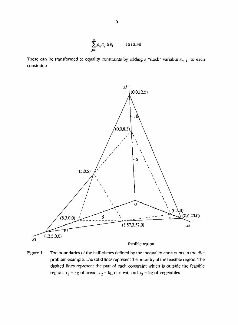
is small. Figure 1 gives the boundaries of the half-planes defined by the inequality constraints
in the diet problem example. The feasible region is generated by the intersection of a finite
number of half planes that form a closed, convex polyhedral set. If the objective function is
evaluated at each of the extreme points of the feasible region in Figure 1 then the extreme point
(3.57,3.57,0) yields the minimum value for the objective function of 17.85 and is thus, the
optimum solution for the diet problem. The optimum solution gives a minimum cost diet which
contains 3.57 kg of bread, 3.57 kg of meat and 0.00 kg of vegetables. This diet provides 200
calories and 400 mg of vitamins at a cost of $17.85. This example illustrates two important
features of linear programs: first the optimal feasible solution will always occur at an extreme
point if a feasible solution exists; second, a basic feasible solution is a feasible solution with no
more than m non-zero Xj. For example, in Figure 1 all the feasible extreme points have no more
than two non-zero values.
The theories relating to linear programming depend on the model being represented in a
normal form where the all the constraints are represented as linear equalities and the variables
are all non-negative. This enables the procedure based on Gauss-Jordan elimination to be used
to solve linear programming problems. Any linear problem's inequality constraints can be
transformed into an equality constraint by the addition of slack or the subtraction of surplus
variables to the original inequality constraints. The cost coefficients in the objective function for
the slack and surplus variables are given a value of zero. Consider the following set of inequality
constraints:
Table 1. Food composition and costs for the diet problem
calories per kg vitamin mg per kg cost per kg
Bread 24 8 2
Meat 32 20 3
Vegetable 16 12 2
6
n
^aijXj<bi l</<wl ;=i
These can be transformed to equality constraints by adding a "slack" variable to each
constraint:
(0,0,12.5)
(0,0,8.3)
(5,0,5)
(0,10) (0,6.25,0) (8.3,0,0) '
(3.57,3.57,0)
(12.5,0,0)
feasible region
Figure 1. The boundaries of the half-planes defined by the inequality constraints in the diet
problem example. The solid lines represent the boundry of the feasible region. The
dashed lines represent the part of each constraint which is outside the feasible
region. .Vj = kg of bread, x^ = kg of meat, and .V3 = kg of vegetables

7
% OijXj + x„+i = bi \<i<ml [4] v=i
where is considered to have taken up the slack in the original inequality constraint. Similarly,
consider the set of inequality constraints:
n
^ aijXj > bi ml +1 < / < ml
M
These can be transformed by subtracting a "surplus" variable to give:
n
^OijXj - x„+i = bj ml + l<i<m2 [5] 7=1
where is considered to have removed the surplus in the original inequality constraint.
Variables in the original linear programming problem which are not subject to the non-negativity
constraints can be expressed as the difference between to positive variables to transform the
linear program to normal form. For example:
if Xi e91 thenx; =X2-x^ 3X2,xi>Q
To transform the linear program, X2 and A'3 are substituted for x^ in the original linear
programming problem. For example, in the diet problem the linear program may be expressed
in normal form as:
min z = 2xi+ 3x2 + 2x3
s. t. 24 + 31X2 +1 6a'3-X4 = 200
8^1 +20A.'2 + 12A'3 — Xg = 100
A-i,X2,.V3,;f4,JC5 > 0
where x^ and Aj are surplus variables.
The linear programming problem is written in matrix notation in normal form as:
min z = c'x
s.t. Ax = b
x > 0 [ 6 ]
where c is an (jx x 1) vector, A is an (m x /;) matrix, b is an (w x 1) vector, and x is an (/i x 1)
vector of variables including surplus and slack variables. The feasible set S can be denoted as:
5 = {x|Ax = b,x>0} [7]

8
which allows an n dimensional extreme point, say x, to be defined mathematically as:
x.y.zeSandzTiy thenx?iay+(l-a)z 0<a<l [8]
Several methods are available for solving linear programs such as complete description
(Pfaffenberger and Walker, 1976), simplex method (Dantzig, 1951), Lagrangian multipliers
(Sposito, 1989), and Karmarkar's procedure (Karmarkar, 1984). Only the simplex method and
Karmarkar's procedure are suitable computational tools for large linear programming problems.
Karmarkar's procedure is an interior algorithm that is claimed to be faster than the simplex
method (Karmarkar, 1984). The procedure involves finding an interior feasible solution which
is transformed such that the solution is near the center of the transformed feasible region. Then
a projection in the direction of steepest descent is used to identify a new interior solution close
to the boundary of the feasible region which improves the objective function. Then new interior
feasible solution is transformed and the procedure continues iteratively until the projection
distance is sufficiently small indicating that the interior feasible solution is at the optimal extreme
point. Variants on Karmarkar's original algorithms have been suggested by Gray (1987) and Todd
(1988). There is no evidence to suggest that this method is computationally more efficient than
the simplex method for large practical linear programming problems.
The simplex method has been widely used for solving large linear programs. It was used
to solve the linear programs in this study and is therefore discussed in detail.
Simplex method for solving linear programs
The simplex method is based on solving a system of over-determined equations using Gauss-
Jordan elimination. The simplex method consists of constructing a feasible solution first and then
finding a maximum (or minimum) feasible solution.
Define ay as the yth column vector of A, and denote B as an (m x m) nonsingular matrix whose
columns are any set of m linearly independent columns vectors of A, say vectors to a„,. The
columns of B form a basis in w-dimensional space, hence B is denoted as the basis and any
column of A can be expressed as a linear combination of the column vectors in B. If a feasible
solution exists with m non-zero points then this is defined as a basic feasible solution. A basic
feasible A can be partitioned into A = [B B] where B is a matrix containing the non-basic
columns of A, a„,+i to a„. In addition there exist scalars such that:
m a^ = %.a/ m<k<n [91
(=1
If A, is the basic feasible solution associated with the basis B then:

9
AA,=[B B]A,=[B B] ^6 = b
where = 0 since X is a basic feasible solution and hence, BA,^ = b. The cost vector c' can be
partitioned into [c{, c^] where c'^ is the costs corresponding to the basic column vectors in A
and c'„ is the costs associated with the non-basic column vectors in A. Now the objective function
IS:
z — c A, — [10]
A scalar Zj can be defined such that:
^j=^XijCi, j=c'i , \ j 1=1
where Xj is the vector of the elements Xjj, / = 1 to m. The reduced cost for the j th column is then
Zj - Cj which will be used for choosing which column enters a new basis.
Assume that X is also a basic solution. A new basic solution is generated by removing a
column vector from B and replacing it with a column vector from B. If ay is in B then from Eq.
19]:
(=1
[11]
For ay to replace a vector in B to form the new basis in m-dimensional space (new basis is
nonsingular) ,Y,y must be non-zero. Assuming ay replaces a^ then from Eq. [11]:
m ax; =——
^kj ,tl Xkj m< j<n,\<k<m [12]
i^k
Since BX^ = b, by substituting Eq. [12] for a^ gives:
m
1=1
M
^bi^i —
Xkj Xkj m< j<n,\<k<m
which specifies the new basic solution. The new basic solution must be non-negative to be
feasible, hence:

10
^kj [13]
[14] ^kj
The vector moving into the basis must have a coefficient, < 0 for Eqs. [131 and [14] to hold.
If Xjj > 0 for at least one / * k then the choice of column k to be removed from the basis is:
to ensure that Eq. [13] is satisfied.
If the new basic solution is chosen using rule [15] it will be feasible. However to be a useful
solution the objective function must be improved. The new objective function will be:
therefore, the new basic feasible solution will increase the objective (maximizing) if and only
if ~^/t) < 0 since, / Xf-j > 0. Three outcomes are possible when selecting the kth column
to enter the basis:
1. <0 for some k with a,;. > 0 for at least one /—a new basic feasible solution
can be obtained using Eq. [14] which will improve the objective function.
2. {zk~Ck) < 0 for some k, and < 0 for i = 1 m and < 0 for at least one /—
then z will increase without bound. The linear programming problem is unbounded.
3 . ( z ^ - c & ) > 0 f o r a l l k. The current basic feasible solution is optimal.
[15]
[16]

11
Obtaining an initiai basic feasible solution
In the discussion of the simplex method it has been assumed that a basic feasible solution
exists and is known. In many practical linear programs an initial basic feasible solution must be
computed before the simplex method can be used to find the optimal solution. For example,
the diet problem has no obvious initial basic feasible solution. To use the simplex method an
initial feasible solution must be identified. If wj linearly independent (LIN) columns of A can be
identified then, the inverse of the columns multiplied by b will yield an initial feasible solution
provided the resulting values of x are greater or equal to zero. For problems of moderate size
finding m LIN columns which will yield an initial feasible solution by this approach would be
complex and computationally difficult requiring matrix inversion. If there exists m constraints
which form an m x m identity matrix the initial feasible solution can be obtained by setting the
values of x corresponding to the columns in the m x m identity matrix equal to values of b. An
initial basis is formed by the addition of artificial variables to the original problem. The objective
is to form an initial (m x m) basis which is an identity matrix. This is achieved by adding artificial
variables to the equality constraints and to ">" inequality constraints as well as the surplus
variables. The slack variables added to the "<" inequality constraints have coefficients of 1. These
slack variables can be used to form an initial basis without the need for artificial variables. Thus,
any linear programming problem with only "<" inequality constraints will have an initial basis
which can be formed from the slack variables, hence the simplex method can be directly applied
to find an optimal solution with these problems.
A two phase method is widely used to solve linear programs. This dichotomizes the problem
into two phases, with phase I concerned with obtaining a basic feasible solution and phase II
with finding an optimal solution.
Phase I
Assume that the linear programming problem is in normal form and h artificial variables have
been added to identify an initial basic feasible solution, where h is the number of equality and
greater than or equal constraints. The objective of phase I is to use the simplex method to remove
the artificial variables from the basis, thus identifying a basic feasible solution containing the
variables of the original problem. To achieve this objective a pseudo objective function is used:
Z = 0'Xi -rX2 =c'x
where the vector Xj corresponds to the variables in the original problem and the vector *2
corresponds to artificial variables. If this pseudo objective function is maximized then the
maximum will be obtained when X2 = 0. As the pseudo objective function reaches the value of
zero the artificial variables will either have been removed from the basis or be in the basis at
zero level. Three possibilities can occur at the termination of phase I:
12
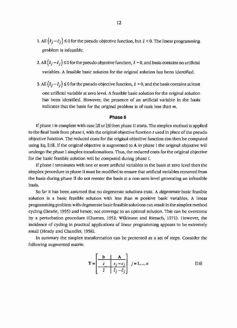
1. All (zy -cy ) < 0 for the pseudo objective function, but z < 0. The linear programming
problem is infeasible.
2. All (zy -cjj<0 for the pseudo objective function, z = 0, and basis contains no artificial
variables. A feasible basic solution for the original solution has been identified.
3. All (zy - cy ) < 0 for the pseudo objective function, z = 0, and the basis contains at least
one artificial variable at zero level. A feasible basic solution for the original solution
has been identified. However, the presence of an artificial variable in the basis
indicates that the basis for the original problem is of rank less than m.
Phase II
If phase I is complete with case [2] or [31 then phase II starts. The simplex method is applied
to the final basis from phase I, with the original objective function z used in place of the pseudo
objective function. The reduced costs for the original objective function can then be computed
using Eq. [10]. If the original objective is augmented to A in phase I the original objective will
undergo the phase I simplex transformations. Thus, the reduced costs for the original objective
for the basic feasible solution will be computed during phase I.
If phase I terminates with one or more artificial variables in the basis at zero level then the
simplex procedure in phase II must be modified to ensure that artificial variables removed from
the basis during phase II do not reenter the basis at a non-zero level generating an infeasible
basis.
So far it has been assumed that no degenerate solutions exist. A degenerate basic feasible
solution is a basic feasible solution with less than m positive basic variables. A linear
programming problem with degenerate basic feasible solutions can result in the simplex method
cycling (Bearle, 1955) and hence, not converge to an optimal solution. This can be overcome
by a perturbation procedure (Charnes, 1952; Wilkinson and Riensch, 1971). However, the
incidence of cycling in practical applications of linear programming appears to be extremely
small (Heady and Chandler, 1958).
In summary the simplex transformation can be presented as a set of steps. Consider the
following augmented matrix:
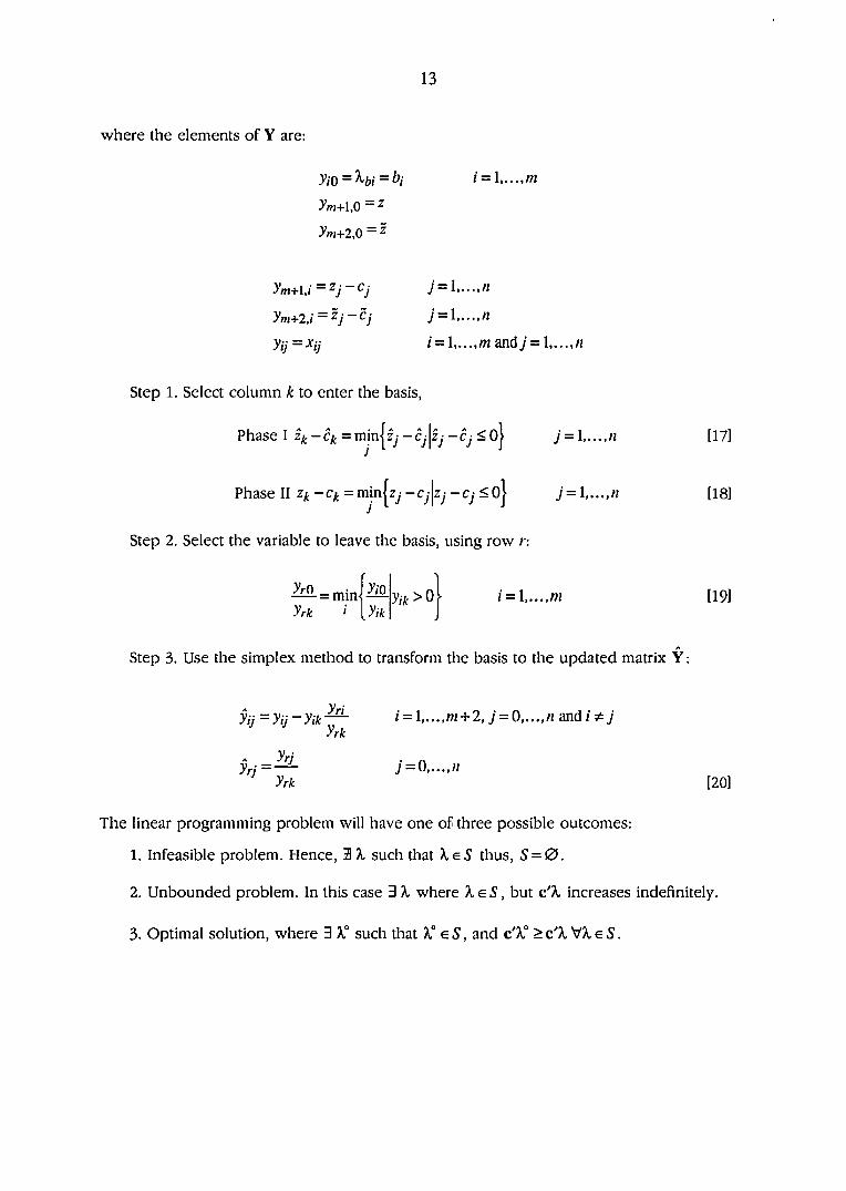
13
where the elements of Y are:
yiO = '^bi=t>i i =
ym+lO=^
ym+2,0 = z
ym+u=^j-Cj y = i n
ym+2 , i=^ j -C j J = yij=Xij i = and; =
Step 1. Select column k to enter the basis,
Phase I Zk-Cfr = minjzy-cy|zy-cj <o| j = [17]
Phase II zi^-Cf. = minjzy -cj zj -cy < o| j = [18]
Step 2. Select the variable to leave the basis, using row n
•^ = mini — yrk ' [yik
i = [191
Step 3. Use the simplex method to transform the basis to the updated matrix Y :
y i j = y i j - y i k — i = l , . . . ,m + 2,j = 0,. . . ,n andi^j yrk
yrj . n yrj=— J = 0.. . . ,n yrk [20]
The linear programming problem will have one of three possible outcomes:
1. Infeasible problem. Hence, 3 X such that thus, S = 0.
2. Unbounded problem. In this case 3 X where X g 5, but c'^ increases indefinitely.
3. Optimal solution, where 3 A,° such that X° eS , and c'A,° >c 'X \ /XeS .

14
An Illustration of the simplex method
Consider the diet problem example:
min z = 2xi + 3x2 + 2x3
s. t. 24jci + 32j:2 +16x3 > 200
8J + 20%2 + 12x3 ^ 100
%i,%2,A:3 ^0
The first step in solving this problem using the two phase simplex method is to represent the
problem in normal form and as maximization problem:
max z = —2xi — 3x2 ~ 2x3
s. t. 24 A'l +32%2+l 6.V3 = 200
8^1 + 20A'2 ^2x3 — Xg =100
A1,-V2,-Ï3,.V4,J:5 >0
Two surplus variables x^ andxg have been included to allow both of the constraints to be written
as equality constraints. It is not possible to identity an initial feasible solution by inspection. Two
artificial variables and Xy are required to find an initial basic feasible solution. The artificial
variables are added to each of the constraints giving:
max z = -2xi- 3-^2 ~ 2x3
s . t. 24,Vi +32^2+16.Y3+%6 = 200
8A'i + 20%2 +12%3 — A'5 + A7 = 100
Xi, A2,JC3,X4,A-5,.V6,A7 > 0
A pseudo objective function for phase I is f = -A'7-A^.To illustrate the simplex transformations,
Tableaus representing the Y matrix will be used. The initial Tableau is:
Tableau 1
basis b ^1 X2 -V3 A4 ^5 ^6 Xl
^6 200 24 32 16 -1 0 1 0
100 8 20 12 0 -1 0 1
z 0 2 3 2 0 0 0 0
z -300 -32 -52 -28 1 1 0 0

15
where the reduced costs for jCj tox-y for the pseudo objective function are computed using Eq.
[10].
First, select the column to enter the basis using Eq. [17]. The column corresponding to X2
has the minimum reduced cost of -52, thus X2 selected to enter the basis. Second, identify the
variable to leave the basis from Eq. [19]. This involves finding the minimum for yiQ / >>22 ( = 1,2,
(i.e., min { 200/32, 100/20 ) ). The row corresponding to Xy is selected to leave the basis. Last,
transform Tableau 1 using Eqs. [20] and [21] where k=2 and r=2 giving:
Tableau 2
basis b ^3 X4 Z5 X6
X6 40 11.2 0 -3.2 -1 1.6 1 -1.6
Xl 5 0.4 1 6 0 -.05 0 .05
z 15 8 0 2 0 .15 0 -.15
z -40 -11.2 0 3.2 1 -1.6 0 2.6
where the new basis consists of xg and Xg Two columns are candidates to enter the basis in
Tableau 2—columns corresponding to Xj, and X5 Choose the column responding to x^ then,
xg is the variable to leave the basis (row 1). Now, transform Tableau 2 with k = 5 and r = 1 giving:
Tableau 3
basis b ^1 -^3 A-4 ^5 ^6
'^6 25 7 0 -2 -.625 1 ^25 -1
^5 6.25 .75 1 .5 -.031 0 .031 0
z 18.75 -.25 0 0.5 .094 0 -.094 0
z 0 0 0 0 0 0 1 1
where the new basis consists of Xg andX2- Observe that there are no artificial variables in the basis
in Tableau 3 and that the pseudo objective function has value zero. This indicates that a basic
feasible solution to the initial problem has been identified, hence phase I is complete. It is no
longer necessary to include the pseudo objective function row or the artificial variable columns
in the Tableau for Phase II. The simplex procedure continues, with the original objective row
used to determine the column to enter the basis.
The column corresponding to is the only candidate to enter the basis and row 2
corresponding to Xg will leave the basis. The transformed Tableau is:
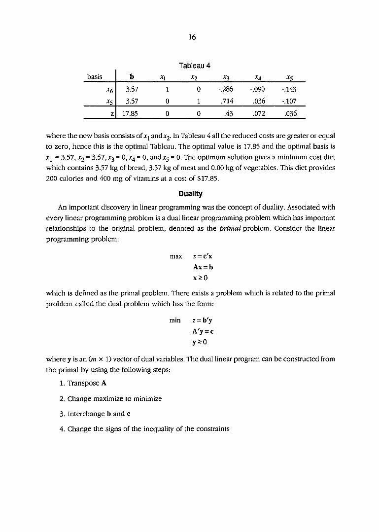
16
Tableau 4
basis b ^1 ^3 H
^6 3.57 1 0 -.286 -.090 -.143
^5 3.57 0 1 .714 .036 -.107
z 17.85 0 0 .43 .072 .036
where the new basis consists of and j:2. In Tableau 4 all the reduced costs are greater or equal
to zero, hence this is the optimal Tableau. The optimal value is 17.85 and the optimal basis is
Xi = 3.57, = 3.57, X) = 0, j:4 = 0, andxg = 0. The optimum solution gives a minimum cost diet
which contains 3.57 kg of bread, 3.57 kg of meat and 0.00 kg of vegetables. This diet provides
200 calories and 400 mg of vitamins at a cost of $17.85.
Duality
An important discovery in linear programming was the concept of duality. Associated with
every linear programming problem is a dual linear programming problem which has important
relationships to the original problem, denoted as the primal problem. Consider the linear
programming problem:
max z = c'x
Ax = b
x > 0
which is defined as the primal problem. There exists a problem which is related to the primal
problem called the dual problem which has the form:
min z = by
A'y = c
y > 0
where y is an (jni x 1) vector of dual variables. The dual linear program can be constructed from
the primal by using the following steps:
1. Transpose A
2. Change maximize to minimize
3. Interchange b and c
4. Change the signs of the inequality of the constraints

17
For example, if the diet problem is considered as the dual problem then, there exists a primal
problem. Using steps [1] to [4] the primal problem for the diet example would be:
max z = 200>'i +100>'2
s.t. 24)'i+83'2^2
32yi +20y2 ^ 3
16^1 +12^2 — 2
Using steps [1] to [4] it can be observed that the dual of the dual problem is the primal problem
and vice-versa. Furthermore, if xe{x|Ax<b,x>0}, y G{y|A'y>c,y>0}, and c'x = b'y then it
can be shown that x is the optimal solution to the primal problem and y is the optimal solution
to the dual problem.
Duality is important in the development of the duality theorem and the existence theorem
of linear programming. These theorems establish sufficient conditions that ensure the dual and
primal problems both have optimal solutions. A relationship exists between the ith primal
constraint and the /th dual variable and vice-versa which known as complementary slackness.
Complementary slackness states that feasible vectors x and y are optimal if and only if:
y/ > 0 then (Ax)y = 6, [21]
and:
xi > 0 then (A'y). = c/ [22]
This relationship can be derived as part of the Kuhn-Tucker optimal ity conditions (Kuhn and
Tucker, 1950) which are the conditions required for the existence of a saddle point solution to
the saddle value problem related to the primal and dual problems. The Lagrangian of the primal
problem is:
<E)(x,y) = c'x + y'(b-Ax) [23]
and the associated saddle value problem is:
find vectors x° > 0, and y° > 0 such that
o(x,y°)<ct)(x°,y°)<<[)(x°,y) x,y>0
If x° and y° are saddle point solutions then:

18
a. x°>0
b. />0
c. b-Ax'>Q
d . c - A y < 0
e. y°{b-Ax''^ = 0
f . A ' > ' ° j = 0
where [a] though \f\ are identical to the Kuhn-Tucker optimality conditions derived using the
Lagrangian multipliers of classical optimization. The conditions [e] and [f\ are complementary
slackness conditions. If a saddle value solution exists then the Kuhn-Tucker optimality
conditions will be satisfied. Also the saddle value solution is the optimal solution to the primal
and dual problems. Furthermore, with the use of Karlin's Lemma (Karlin, 1959) in conjunction
with the saddle value problem it is possible to show that if there exists an optimal solution to
either the dual or primal problem then there necessarily exists a solution to the corresponding
primal or dual problem and the optima are equal. A full discussion and proofs of the duality
theorem and the existence theorem of linear programming are given by Sposito (1989).
The dual variables have an economic interpretation. Consider the primal problem where the
b denotes the availability of resources. If the ith resource, bj, is increased by A the dual objective
function becomes:
m {bi+A)yi+'^bjyj
e
where the dual variable y,- is the rate of change in the primal objective function from a unit
increase in the /th resource. The dual variable y^can be considered as the marginal cost or return
for a A increase in the /th resource. If a resource is not completely utilized by the system, that
is, there is surplus resource over requirements, then the law of supply and demand would
suggest that the marginal value of a unit increase in that resource should be zero. This
relationship holds under duality via complementary slackness:
y° (b-Ax°j = 0

19
since b-Ax° >0 when there is a resource surplus, hence y° =Ofor complementary slackness
to hold.
Linear duality theory has lead to the development of the primal-dual and the dual simplex
methods for solving linear programming problems. These methods avoid the need for a two
phase implementation of the simplex algorithm by simultaneously finding a feasible solution
and an optimal solution. These methods may be computational more efficient for certain classes
of linear programming problems. For example, the dual simplex is more efficient than the
simplex method for problems that are in the dual form such as the diet problem. However, the
dual simplex offers no advantage over the simplex method if the simplex method is used to
solve the primal form of the diet problem.
It is desirable to maximize the computational efficiency of the algorithms used to solve large
linear programming problems. This section will discuss three improvements to the simplex
method: optimal pivoting, identification of redundant non-basic variables and transformation
of lower bounds.
The choice of column to enter the basis only requires that the reduced cost is less than zero.
In most practical situations there may be a number of columns which meet these criteria. Optimal
pivoting provides an objective procedure for choosing which column should enter the basis.
The criterion is to choose the column which will result in the largest gain in the objective function
for a given iteration. The change in the objective function from the kth column entering the basis
is:
from Eq. [l6]. This can be maximized by choosing k such that:
Optimal pivoting will increase computational effort for each iteration, by requiring the
calculation of "^bk^^kj * where (z^.-Cyt)<0. However, optimal pivoting usually
substantially reduces the total number of iterations required to solve the problem which
increases the overall computational efficiency.
The optimal solution has n-m variables that are non-basic. If variables which will be non-
basic in the optimal solution could be identified and eliminated during the simplex procedure,
Further computational considerations
[24]
20
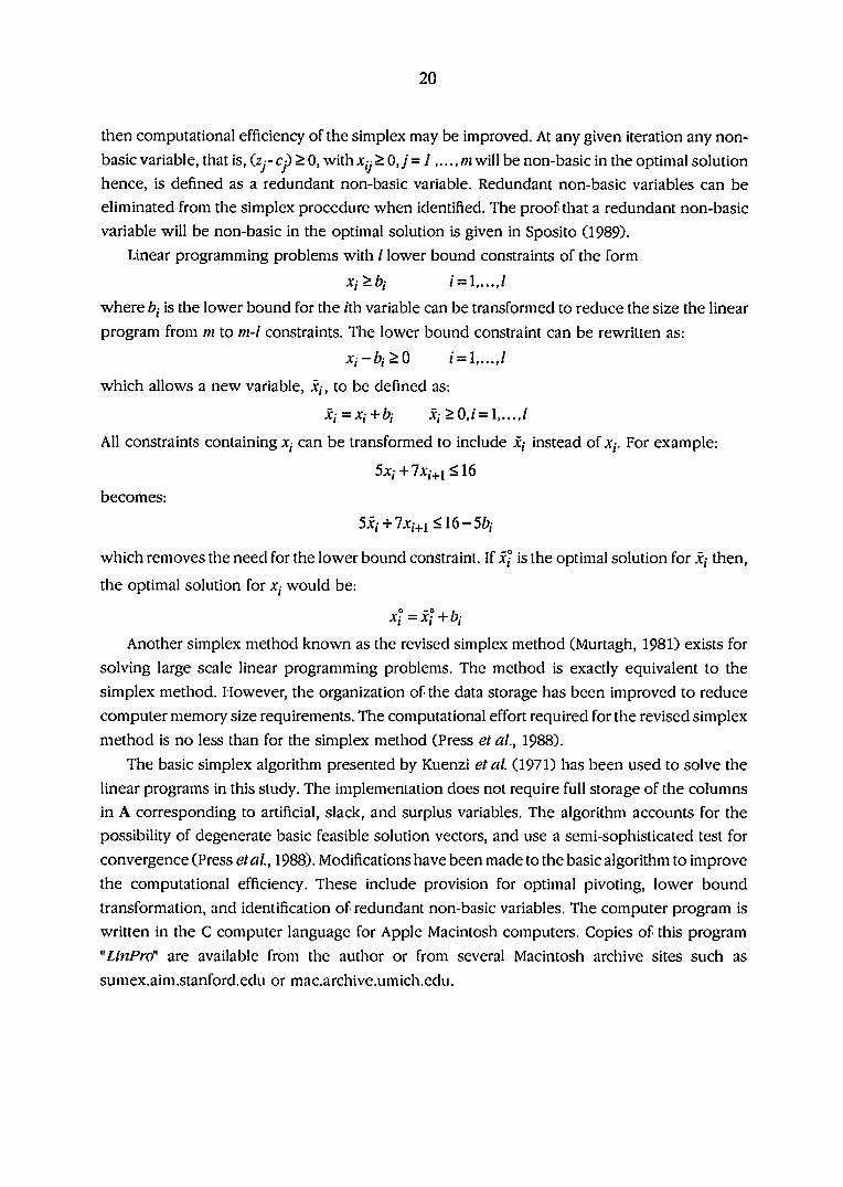
then computational efficiency of the simplex may be improved. At any given iteration any non-
basic variable, that is, (zy- Cy) > 0, with > 0,y = 7 , m will be non-basic in the optimal solution
hence, is defined as a redundant non-basic variable. Redundant non-basic variables can be
eliminated from the simplex procedure when identified. The proof that a redundant non-basic
variable will be non-basic in the optimal solution is given in Sposito (1989).
Linear programming problems with / lower bound constraints of the form
Xi>bi / =
where 6, is the lower bound for the ith variable can be transformed to reduce the size the linear
program from m to m-l constraints. The lower bound constraint can be rewritten as:
xi—bi^O i =
which allows a new variable, x,-, to be defined as:
Xi = Xi + bi Xi>0,i = l,...,l
All constraints containing x, can be transformed to include Jf,- instead of Xj. For example:
5xi+lxi+i <16
becomes:
Sx j 4- I x - f ^ i < 16—56/
which removes the need for the lower bound constraint. If x} is the optimal solution for then,
the optimal solution for would be:
x} = x°i + bj
Another simplex method known as the revised simplex method (Murtagh, 1981) exists for
solving large scale linear programming problems. The method is exactly equivalent to the
simplex method. However, the organization of the data storage has been improved to reduce
computer memory size requirements. The computational effort required for the revised simplex
method is no less than for the simplex method (Press et ai, 1988).
The basic simplex algorithm presented by Kuenzi et al. (1971) has been used to solve the
linear programs in this study. The implementation does not require full storage of the columns
in A corresponding to artificial, slack, and surplus variables. The algorithm accounts for the
possibility of degenerate basic feasible solution vectors, and use a semi-sophisticated test for
convergence (Press etal., 1988). Modifications have been made to the basic algorithm to improve
the computational efficiency. These include provision for optimal pivoting, lower bound
transformation, and identification of redundant non-basic variables. The computer program is
written in the C computer language for Apple Macintosh computers. Copies of this program
"LinPro" are available from the author or from several Macintosh archive sites such as
sumex.aim.stanford.edu or mac.archive.umich.edu.

21
References
Bearle, E. M. L. 1955. Cycling in the dual simplex algorithm. Nav. Res. Logist. Quarterly. 2:269.
Charnes, A. 1952. Optimality and degeneracy in linear programming. Ecotiometrica.
2:160.
Dantzig, G. B. 1951. Maximization of a linear function of variables subject to linear inequalities.
In Activity Analysis of Production Allocation. John Wiley and Sons, Inc., New York.
Dorfman, R., P. A. Samuelson, and R. W. Solow. 1958. Linear programming and economic
analysis. McGraw Hill, New York.
Gray, D. 1987. A variant of Karmarkar's linear programming algorithm for problems in standard
form. Mathematical Programming. 37:81.
Hadley, G. 1962. Linear Programming. Addison-Wesley, Reading, Mass.
Heady, E. O., and E. O. Chandler. 1958. Linear programming Metljods. Iowa State Press, Ames,
lA.
Karmarkar, N. 1984. A new polynomial algorithm for linear programming. Combinatorica. 4:373.
Karlin, S. 1959. Mathematical methods and theory of games, programming and economics.
Addison-Wesley, Reading, Mass.
Kuhn, H. W, and A. W. Tucker. 1950. Nonlinear programming. Second Symp. Proc. on
Mathematical Statistics and Probability. Univ. of California Press, Berkeley, Calif.
Kuenzi, H. P., H. G. Tzschach, and C. A. Zehnder. 1971. Numerical Methods of Mathematical
Optimization. Academic Press, New York.
Murtagh, B. A. 1981. Advanced linear programming. McGraw Hill, New York.
Pfaffenberger, R. C., and D. A. Walker. 1976. Mathematical Programming for Economics and
Business. Iowa State Press, Ames, lA.
Press, W. H., B. P. Flannery, S. A. Teukolsky, and W. T. Vetterling. 1988. Numerical Recipes in
C. ne Art of Scientific Computing. Cambridge Univ. Press, Cambridge, UK
Saaty, T. L. 1988. Mathematical Methods of Operations Research. Dover Publ. Inc., New York.
Sposito, V. A. 1989. Linear Programming with Statistical Applications. Iowa State Press, Ames, lA.
Todd, M.J. 1988 Polynomial algorithms for linear programming. In Advances in Optimization and
Control, ed Eisett, H. A., and G. Pederzoli. Springier Verlag, Berlin.
Wilkinson, J. H., and C. Reinsch. 1971. Linear Algebra, vol II of Handbook for Automatic
Computation. Springier Verlag, Berlin.

22
PART II. THE ECONOMIC VALUE OF GENETIC GAIN FROM DAIRY
SIRE SELECTION
23
INTRODUCTION
Part II of this dissertation describes a method for determining the economic value of
response to selection utilizing a farm level linear programming model. To enable modelling
response to selection at the farm level methods for estimating response to selection and genetic
and phenotypic (co)variances are required. The literature review summarizes methods for
estimating the response to selection, multiple stage selection index and methods that have been
used to derive economic weights for selection index. Paper 1 derives general equations for
predicting response to selection accounting for multiple stage selection with overlapping
generations. A example application of these methods to a dairy progeny testing scheme is
discussed. A FORTRAN 77 computer program which uses these equations to compute the
response to selection accounting for multiple stage selection with overlapping generations is in
Appendix 3.
Nine traits were included in the linear programming farm model, namely: milk yield, fat
yield, protein yield, somatic cell score, liveweight, days open, stature, body depth and udder
depth. Milk, fat and protein yields were selected because they represent the primary produce
of the enterprise. Somatic cell score was selected because it is considered a useful selection
criterion for the incidence of mastitis. Liveweight was considered because it is an important
component of economic efficiency of dairy cattle. Days open was considered since it is one of
the best documented of the fertility traits and is a measure for efficiency of female fertility. Finally,
the three linear type traits were valued by their actions on herdlife. To predict responses to
selection for the nine traits using the equations outlined in Paper 2 estimates of genetic and
phenotypic (co)variance components are required. Recent estimates of genetic and phenotypic
(co)variances for the nine traits are summarized in the literature review.
Paper 2 describes the farm level linear programming model. The model is used to determine
optimal rates of genetic gain for each of the nine traits for four planning horizons. The linear
programming model is used to determine relative economic weights for the nine traits.
Appendices 1 and 2 give a detailed account of the linear programming model with a numerical
example of the constraints. Appendix 4 provides a Mathematica program for computing
constraints from bivariate normal contours.
24
LITERATURE REVIEW
Response to selection
The change in a population mean produced by artificial selection is known as the response
to selection denoted, by R. The selection response is defined as the difference in mean
phenotypic value between the offspring of selected parents and the phenotypic mean of all
possible parents. The mean of individuals selected as parents expressed as a deviation from the
population mean is known as the selection differential (5). When the parents are ranked from
highest to lowest phenotype and the highest 1 to/: individuals being selected then S is defined
as:
k
ly:
5 = - f c | X [ 1 1 k
where >>,• is the phenotypic value of the selected ith parent and y is the population mean.
Assuming there is no natural selection, and the fertility and viability of the individuals are not
correlated with the phenotypic value of the character of interest, the response to mass selection
is given by (Falconer, 1989):
^ ~ [2]
where is b^p the regression of offspring on mid-parent phenotypic value. Equivalently the
response to mass selection can be defined as:
R = h^S [3]
where is the heritability in the narrow sense, defined as the ratio of additive genetic variance
to phenotypic variance:
h~=^- [4] Op
The selection differential can be predicted in advance provided that two conditions hold—
selection is by truncation, and the phenotypic values are normally distributed. The standardized
selection intensity is defined as:

25
where Xi is the standardized order statistic xi=(yi-y.)ICp. The approximate predicted
selection intensity can be found for large k from the expected values of the truncated normal
distribution. Let X be a standard normal variate truncated at z (values below z being discarded).
The density function of X is:
where p is the proportion selected:
•(x>z) [6]
-i,
and:
E(x) = [8] P
The expected values for order statistics have been extensively tabulated (see Fisher and Yates,
1953). For small values of k Eq. [8] overestimates /. A better approximation for i is obtained by
defining p (Bulmer, 1981) as:
p = (k+^)l(n + -^) [9] 2 2/1
where n is the number selected. The expected response to selection from Eq. [2] can then can
expressed as:
R = ih~ap=ihc5a [11]
Equation [11] assumes selection on individual performance and discrete generations. Dickerson
and Hazel (1944) provided original formulae for predicting the rate of response to selection in
overlapping generations which were generalized by Rendel and Robertson (1950). Selection in
the male and female are further sub-divided to distinguish four intensities of selection and four
generation intervals according to the following reproductive pathways:
1. males to produce males
2. males to produce females
3. females to produce females
4. females to produce males
26
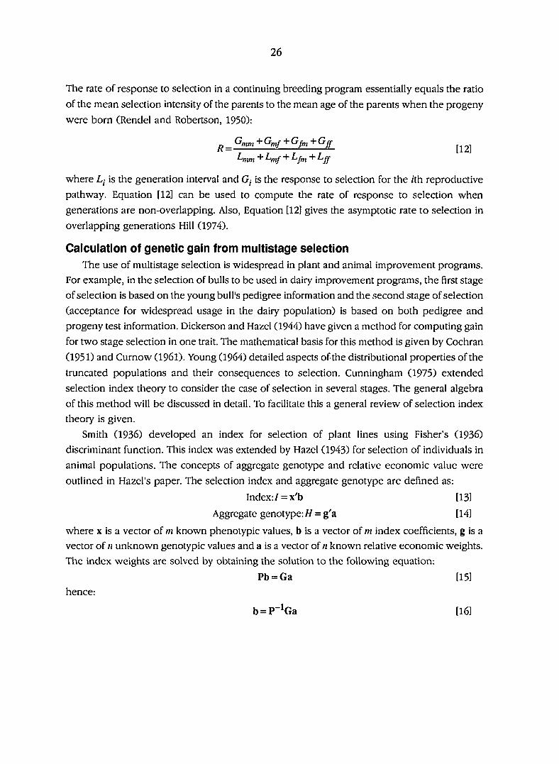
The rate of response to selection in a continuing breeding program essentially equals the ratio
of the mean selection intensity of the parents to the mean age of the parents when the progeny
were born (Rendel and Robertson, 1950):
where L, is the generation interval and G,- is the response to selection for the /th reproductive
pathway. Equation [12] can be used to compute the rate of response to selection when
generations are non-overlapping. Also, Equation [12] gives the asymptotic rate to selection in
overlapping generations Hill (1974).
Calculation of genetic gain from multistage selection
The use of multistage selection is widespread in plant and animal improvement programs.
For example, in the selection of bulls to be used in dairy improvement programs, the first stage
of selection is based on the young bull's pedigree information and the second stage of selection
(acceptance for widespread usage in the dairy population) is based on both pedigree and
progeny test information. Dickerson and Hazel (1944) have given a method for computing gain
for two stage selection in one trait. The mathematical basis for this method is given by Cochran
(1951) and Curnow (1961). Young (1964) detailed aspects of the distributional properties of the
truncated populations and their consequences to selection. Cunningham (1975) extended
selection index theory to consider the case of selection in several stages. The general algebra
of this method will be discussed in detail. To facilitate this a general review of selection index
theory is given.
Smith (1936) developed an index for selection of plant lines using Fisher's (1936)
discriminant function. This index was extended by Hazel (1943) for selection of individuals in
animal populations. The concepts of aggregate genotype and relative economic value were
outlined in Hazel's paper. The selection index and aggregate genotype are defined as:
where x is a vector of m known phenotypic values, b is a vector of m index coefficients, g is a
vector of n unknown genotypic values and a is a vector of n known relative economic weights.
The index weights are solved by obtaining the solution to the following equation;
_ G„,„, + G„,f + Gf„t + Gff
^mm + + fm + % [12]
Index:/= x'b
Aggregate genotype:// = g'a
[13]
[14]
Pb = Ga [15]
hence:
b = p-^Ga [16]
27
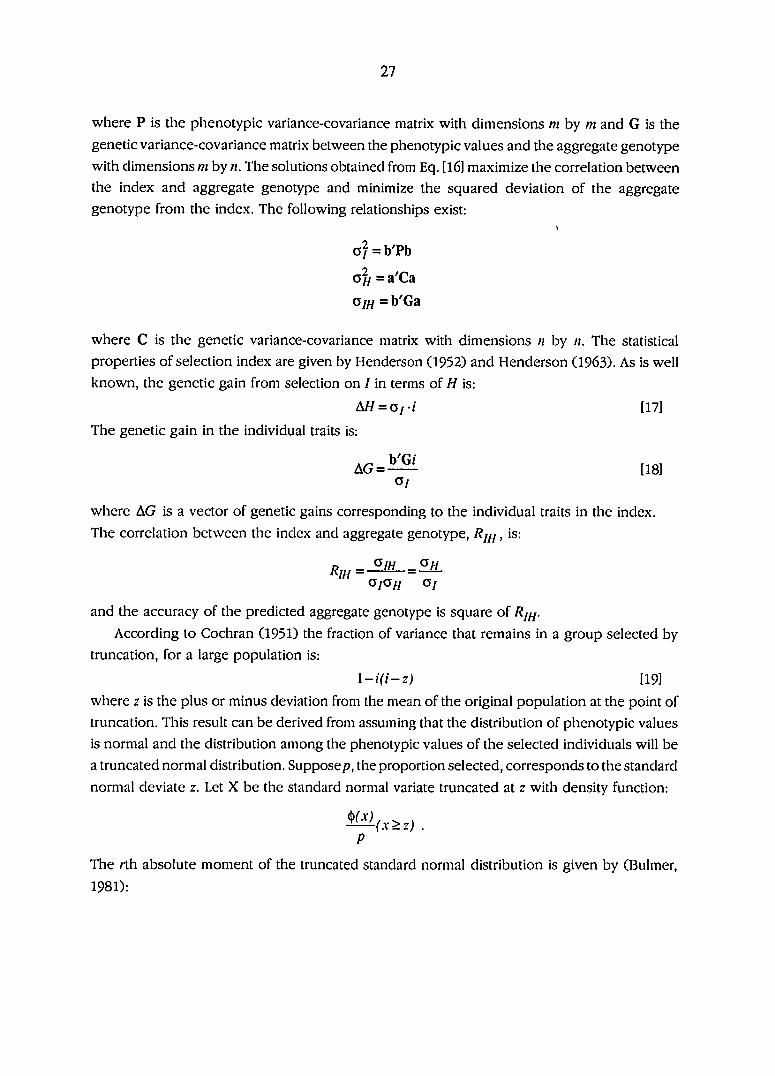
where P is the phenotypic variance-covariance matrix with dimensions m by m and G is the
genetic variance-covariance matrix between the phenotypic values and the aggregate genotype
with dimensions m by n. The solutions obtained from Eq. [l6] maximize the correlation between
the index and aggregate genotype and minimize the squared deviation of the aggregate
genotype from the index. The following relationships exist: t
G/=b'Pb
= a'Ca
a/// =b'Ga
where C is the genetic variance-covariance matrix with dimensions ii by n. The statistical
properties of selection index are given by Henderson (1952) and Henderson (1963). As is well
known, the genetic gain from selection on I in terms of H is:
AH = aj-i [17]
The genetic gain in the individual traits is:
AG = -^ [18]
where AG is a vector of genetic gains corresponding to the individual traits in the index.
The correlation between the index and aggregate genotype, , is:
and the accuracy of the predicted aggregate genotype is square of Rj^.
According to Cochran (1951) the fraction of variance that remains in a group selected by
truncation, for a large population is:
[19]
where z is the plus or minus deviation from the mean of the original population at the point of
truncation. This result can be derived from assuming that the distribution of phenotypic values
is normal and the distribution among the phenotypic values of the selected individuals will be
a truncated normal distribution. Supposep, the proportion selected, corresponds to the standard
normal deviate z. Let X be the standard normal variate truncated at z with density function:
p
The /th absolute moment of the truncated standard normal distribution is given by (Bulmer,
1981):
28
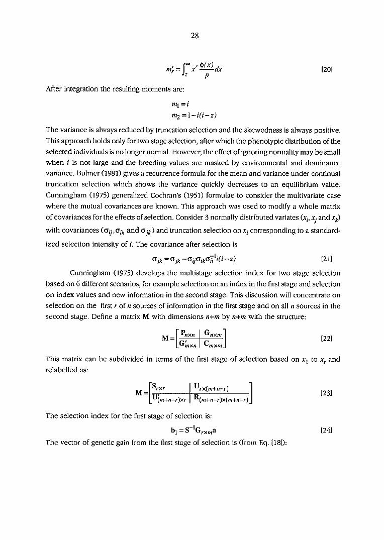
J z p [20]
After integration the resulting moments are:
nil - '
m2 = l-i(i-z)
The variance is always reduced by truncation selection and the skewedness is always positive.
This approach holds only for two stage selection, after which the phenotypic distribution of the
selected individuals is no longer normal. However, the effect of ignoring normality may be small
when i is not large and the breeding values are masked by environmental and dominance
variance. Bulmer (1981) gives a recurrence formula for the mean and variance under continual
truncation selection which shows the variance quickly decreases to an equilibrium value.
Cunningham (1975) generalized Cochran's (1951) formulae to consider the multivariate case
where the mutual covariances are known. This approach was used to modify a whole matrix
of covariances for the effects of selection. Consider 3 normally distributed variates (x,-, Xj and X/)
with covariances (G,y,a,/. and Oy/.) and truncation selection onx, corresponding to a standard
ized selection intensity of /. The covariance after selection is
Cunningham (1975) develops the multistage selection index for two stage selection
based on 6 different scenarios, for example selection on an index in the first stage and selection
on index values and new information in the second stage. This discussion will concentrate on
selection on the first r of n sources of information in the first stage and on all n sources in the
second stage. Define a matrix M with dimensions n+m by n+m with the structure:
^nxn ^nxm
^n ixn ^mxm
This matrix can be subdivided in terms of the first stage of selection based on a'| to x^. and
relabelled as:
O j k i p i k ^ n ^ ( i - z ) [21]
Urx(m+n-r) [23]
•(ni+n-r)x(ni+n-r)
The selection index for the first stage of selection is:
bj — S 'G;.x„,a rxni^ [24]
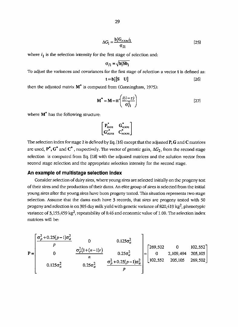
The vector of genetic gain from the first stage of selection is (from Eq. [18]):
29
G/1 [251
where /j is the selection intensity for the first stage of selection and:
O/i =^b'iSbi
To adjust the variances and covariances for the first stage of selection a vector t is defined as:
t = b'i[S U] [26]
then the adjusted matrix M* is computed from (Cunningham, 1975):
M =M-tt'
where M* has the following structure:
o/i [27]
P* G* *^nxn ^nxm G'„ mxn ••mxni
The selection index for stage 2 is defined by Eq. [16] except that the adjusted P, G and C matrices
are used, P*, G* and C* , respectively. The vector of genetic gain, AG2, from the second stage
selection is computed from Eq. [18] with the adjusted matrices and the solution vector from
second stage selection and the appropriate selection intensity for the second stage.
An example of multistage selection index
Consider selection of dairy sires, where young sires are selected initially on the progeny test
of their sires and the production of their dams. An elite group of sires is selected from the initial
young sires after the young sires have been progeny tested. This situation represents two stage
selection. Assume that the dams each have 3 records, that sires are progeny tested with 50
progeny and selection is on 305 day milk yield with genetic variance of 820,419 kg^, phenotypic
variance of 3,155,459 kg^, repeatability of 0.46 and economic value of 1.00. The selection index
matrices will be:
aj+0.25(p-l)o^
P =
P
0
0.125o^
0^(1 +(/i-l)/-)
0.25a;
0A25a~â
0.25al
al+0.25{ p -l)al
269,502 0 102,552
0 2,109,494 205,105
102,552 205,105 269,502

30
'0.25GI' '205,105' G = O.Sal = 410,209
0.5Oo 410,209
C = [a2] = [820,419]
where p is the number of progeny in a progeny test, n is the number of lactations for the dam,
and r is the repeatability. The matrix M is formed as:
'269,502 0 102,552 205,105
P G 'S u' 0 2,109,494 205,105 410,209
G' C U' R 102,552
205,105
205,105
410,209
269,502
410,209
410,209
820,419
where S represents the phenotypic covariance matrix between the sire progeny test, the dam's
average production and the young sires breeding value. Tlie index coefficients for the first stage
of selection from Eq. [24] are:
b] =
The correlation between the aggregate genotype and the index is 0.54 giving the selection index
an accuracy of 0.29. Assume the first stage selection intensity is 2.268, with a point of truncation
of 1.881 and the second stage selection intensity is 1.553. The genetic gain from the first stage
of selection from Eq. [25] is:
'0.761" '269,502 0 " -1 205,105
0.203 0 2,109,494 410,209
AGi =[0.761 0.203] 205,105
410,209 2.268
489.30 = 1110 Isg.
To adjust the genetic and phenotypic covariances for the first stage of selection Eq. [26] is used
to compute the vector t;
t = [0.761 0.203] "269,502 0 102,552
0 2,109,494 269,502
then the matrix M* is computed from Eq. [27] as:
= [205,105 410,209 119,709 239,419]

31
(489.30r
• 115,277 -308,450
-308,450 1,402,595
12,539 25,078
25,078 50,155
12,539 25,078'
25,078 50,155
216,966 305,136
305,136 610,263
The index coefficients for the selection index including all information on the young sires
accounting for the reduction covariance from first stage selection are:
bo =
The correlation between the index and aggregate genotype is 0.84 giving an accuracy for the
selection index of 0.71. The genetic gain from second stage selection is computed from Eq. [18]
as:
"0.234" " 115,277 -308,450 12,539 • -1 '25,078
0.062 = -308,450 1,402,595 25,078 50,155
1.386 12,539 25,078 216,966 305,136
AG2 =[0.234 0.062 1.386]
• 25,078•
50,155
305,136
1.553 657.20
= 1021 kg
Economic weights for selection index
The definition of the aggregate genotype in the review of selection index procedures
required a vector of known relative economic weights. This section will concentrate on the
reviewing the derivation of economic weights used in the selection index.
A breeding objective can be considered as a function used as the basis of genetic evaluation
hence, if livestock are to be selected as parents of the next generation based on their aggregate
genotype then the aggregate genotype can be considered more broadly as a breeding objective.
Thus, it is necessary to establish whose economic benefit will be improved by the selection
process. Selection decisions which maximize the national or industry level economic benefit
may be less than ideal for the individual producer (Harris, 1970; Moav, 1973; Wilton et cil., 1978;
Miller and Pearson, 1979).
Genetic progress in dairy cattle in the United States is produced by Artificial Insemination
(AI) organizations which are either farmer owned cooperatives or privately owned as opposed
to nationally operated schemes. In a nationally operated scheme, the objective would be to
maximize the net welfare to the nation whilst, ensuring the economic viability of the individual
producer enterprises. This is not the main objective for a cooperative or privately owned

32
breeding scheme. Ultimately, genetic gain made by the AI organizations benefit the dairy
producer as well as the consumer. AI organizations are selling technological change to
producers, primarily semen from highly selected bulls. The adoption of genetic improvement
constitutes a continuous process of change which will affect the net income of the producer
throughout the life of the farm business.
There have been several reports of economic selection indices for dairy cattle, most of which
have been concerned with economic values for milk components. The reported selection
indices fall into two categories (Gibson, 1987): those which omitted the costs of production
(Wilton and Van Vleck, 1968; Brascamp and Minkema, 1972; Anderson etal., 1978; Millers, 1984;
dejager and Kennedy, 1987) overestimating the economic values of the traits, or those which
included these costs (Hanna and Cunningham, 1974; Dommerholt and Wilmink, 1986; Groen
1989a,b; Dado era/., 1990). Compared to the number of reports of economic selection indices
there have been few reports which attempt to formally derive economic weights for a selection
index.
Hazel (1943) when describing an economic weight, stated:
the relative valuefor each trait depends upon the amount by which profit may be
expected to increase for each unit of improvement in that trait
Hazel then suggested a good approximation may be obtained from long-time price or cost
averages. Hazel (1956) redefined this concept of an economic weight, he emphasized that the
economic weight should reflect the net profit which accaies from a unit change in that trait and
that this value should not include net profit accruing from changes in correlated traits.
Moav (1966a, b and c) and Moav and Hill (1966) were among the first to clarify the
relationship between profit functions and selection index. Graphical techniques were used to
express profit as a conditional function of production and reproduction. These graphs were used
to determine the most profitable parental combinations for crossbreeding purposes. Also, the
graphical procedures were used to determine optimal index weights. This showed that the
economic weights for the aggregate genotype could be determined from a profit function.
Gibson (1976) derived economic weights for swine with a full economic model and
optimized the profit by linear programming. The weights were derived from sensitivity analysis.
The sensitivity analysis involved changing the linear program coefficients to represent genetic
improvement in the trait. An economic weight was defined as the change in the profit to the
swine firm per unit of improvement in that trait. Procedures for deriving economic weights when
the optimal mix of activities for the swine enterprise changed due to genetic improvement in
the trait were discussed. The basic procedure was to compute the difference between the
optimal solution for the linear program accounting for genetic change and the optimal solution
for the linear program without genetic change. This difference was divided by the average
number of animals with the trait change to present the economic weight on a per unit basis.
33
Melton et al. (1979) proposed a procedure for estimating economic values where the profit
was expressed as a function of all the inputs. The inputs fall into two categories, those supplied
by the producer and those embodied in the animal. They assumed that the producer wished to
maximize profits. This assumed that the producer chooses an optimal mix of animal traits and
supplied inputs in order to maximize the profit. Profit was differentiated with respect to all the
traits and these partial derivatives were equated to zero. The resulting series of equations
involved the economic values of the traits and their mean values. Assuming the producer knew
the mean levels for the traits then, the economic weights could be derived. Thompson (1980)
discussed the model of Melton etal. (1979), however, the discussion was concerned with Melton
et al.'s numerical example and the sufficient conditions for finding optima. He discussed
procedures for insuring that profit maximization had occurred since equating the partial
derivatives to zero does not guarantee this. However, this added nothing new to the basic
concepts of the original model. The results produced by Melton etal. (1979) could have been
obtained by examining profit expressed as a function of producer supplied inputs and products
from animal production, rather than including animal traits as inputs with implied prices.
Ladd (1982) outlined a product-characteristics approach for deriving economic weights
where genetic improvement was analyzed as technical change. The economic weight for a trait
was determined by considering the change in profit, outputs, and inputs due to per unit genetic
change in the trait assuming prices and costs and all other traits remained constant. Ladd (1982)
found that if the enterprise was maximizing profit before the introduction of new genetic
material (technical change) and one trait is increased through the introduction of the improved
genetic material then the enterprise would adopt this genetic material and continue to maximize
profits. The change in profit divided by the number of units introduced (i.e., number of animals
where the animal is the unit of production sold) was the economic weight for that trait. This was
found to equal the marginal product of the trait improved divided by the number units adopted.
The marginal product was defined as the product of the price for the output and the partial
derivative of the output function with respect to the trait.
James (1982) considered the consequences of deriving economic weights from two
economic measures—returns less costs and returns divided by costs. The relative economic
weights can be derived from examining the partial derivatives. James (1982) found that relative
economic weights derived from the function, returns divided by costs, were dependent on the
means of the inputs and output but not prices and costs and that they were also affected by the
addition of fixed costs. In contrast, the relative economic weights derived from the function,
returns - costs, were dependent on the prices and costs, and not affected by the addition of
fixed costs.
The concept of normal profit was used by Brascamp et al. (1985) to show that economic
weights derived from profit function describing different sectors of the industry gave equivalent
34
economic weights. The procedure involved equating the profit function to zero taking partial
derivatives of the profit function with respect to the trait of interest. Smith et al. (1986) found
that the equivalence between economic weights reported by Brascamp etal. (1985) was a special
case of a more general equivalence between economic weights. Smith etal. (1986) showed that
differences in relative economic weights reported by James (1982) and Moav (1973) could be
eliminated by imposing two conditions on the profit function when deriving the economic
weights:
1. Profit generated by changes in the scale of the enterprise should not be consid
ered when deriving economic weights
2. Resources are used efficiently—changes in output will require proportional
changes in inputs. Fixed costs are assumed to increase with increases in output.
They suggested that economic weights should be derived with either the outputs fixed, inputs
fixed, profit fixed or profit zero. Smith et al. (1986) stated that these conditions underline the
concept that the change in net income from genetic improvement comes from reducing the cost
of production per unit of output not from increases of enterprise scale nor from improvement
of management practices.
Groen (1988) outlined a deterministic static model for the derivation of economic weights
in Dutch dairy cattle. The model considered the selection for milk and beef production traits.
Revenues were generated from the sale of fat, protein and carrier, surplus newborn calves and
cull cows. Costs were from feed concentrates, roughage, labor and fixed costs. Groen (1989a)
derived the economic weight for a trait as the change in profit per average cow lactation year
as a consequence of per unit change in the genetic merit of the herd for that trait. Groen (1989a,
b) discussed the sensitivity of these economic weights to varying production levels and output
restrictions, such as quotas on milk production.
Gibson (1989a) discussed methods for deriving economic weights for milk components
using the Canadian milk market as an example. The procedure was developed for situations
where output restrictions exist in the market place and incorporated the concepts of rescaling
discussed by Smith etal. (1986). The rescaling under fixed output required the total output to
remain constant. The economic weights were derived as the change in profit resulting from a
unit change in yield. Gibson (1989b) noted that in a free market (no output restrictions) the
rescaling was not required. The economic weights were found to vary widely depending
whether a restricted or a free market was assumed.
Keller and Allaire (1990) used a herd production model to derive economic weights for fat,
protein, lactose and carrier for five dairy breeds. Keller and Allaire (1990) stated that the herd

35
model predicted costs and returns while accounting for herd age distribution, phenotypic level
of different age groups and factors such as calving interval and culling rate. The economic
weights were computed as the change in profit or change in returns divided by costs per
kilogram change in herd level of a given milk production trait. It was found that the economic
weights derived from the profit function changed linearly with increases or decreases in costs.
Whereas, the economic weights derived from the returns divided by costs changed non-linearly
and the changes were greater in magnitude.
The studies reviewed for the derivation of economic weights have largely equated the
marginal economic value of unit genetic improvement with varying complexity of economic
models. Little or no work has been reported on the development of economic weights for non
productive traits. A one unit increase in a productive trait due to genetic gain will effect the levels
of genetic gain achieved for other correlated traits non-production traits, such as: herd life,
reproductive traits and health traits. These changes must be considered simultaneously when
evaluating the economic worth of that one unit change. The methods reviewed have only
considered the short term costs and returns from genetic improvement when deriving economic
weights. When evaluating the economic value of genetic gain the flow of genetic improvement
through the producer herd over time should be taken into account. The long term consequences
of selection on all traits of economic importance which will affect future net income of the
enterprise and the ultimate value of the accrued genetic gain for traits being selected. A model
which accounts for the flow of genetic improvement in productive and non-productive traits
overtime is required.
Ideally the model of a farm enterprise should include all sources of revenue and cost so that
the net income (profit) would be accurately predicted. Gibson (1987) criticized economic
weights which had not considered the concepts of rescaling or the use of normal profit, or fixed
input discussed by Smith et al. (1986). Gibson considered these weights to be technically
incorrect. These conditions require assumptions to be made about the optimum number of
animals for the enterprise. When output restrictions are functioning in the industry then
increasing production via genetic gain and as a consequence of this, decreasing animal numbers
can not be assumed to maximize net income. There may be immediate optima with lower rates
of genetic gain for production traits—this needs further investigation. Furthermore, Smith et al.
(1986) state that resources should be used efficiently which requires optimization of the
producer system being modeled. Lastly, increasing fixed costs with increases in productive
output may be inappropriate. Since, decisions concerning structural developments in the
industry which allow expansion in the enterprise size are detached from decisions concerning
optimum use of genetic improvement and changes in productive efficiency. The assumption of
Smith et al. (1986) that increases in production via genetic improvement can be achieved by
increases in animal numbers may be incorrect. For example, a producer maybe unable to
36
increase herd size because of physical limitations on the farm (milking parlor, housing used to
capacity) and the unavailability of capital funds to overcome these limitations.
All the methods reviewed in this section for deriving economic weights make the assumption
that the marginal products for production are near constant, for example the amount of resources
(i.e., labor) required to produce milk remains constant over all levels of production. The linear
programming approach of Gibson (1976) may partially account for changing marginal products
by allowing for different production systems for different production levels. Since genetic gain
accrues over time assuming marginal products remain constant may overestimate the value
genetic gain in the longer term. Equating the marginal net income or profit (net income per one
unit genetic change) to an economic weight assumes the value of the unit genetic gain is
constant.
Modelling of the producer enterprise is necessary since the breeding objective via the
aggregate genotype is to maximize a function of net income of the producer enterprise (Allaire
and Thraen, 1985). For this model to be realistic, constraints on the available resources and
constraints concerning production processes will be required. Genetic improvement is a
continuous process thus, any economic analysis of genetic gain can not be done with a static
model, an intertemporal model will be required. A linear programming approach would enable
the results of selection to be combined with the economics of a producer dairy farm over a
predefined planning horizon. Jansen and Wilton (1984) have discussed the general use of linear
programming to selection in livestock. The authors considered linear programming approach
to have several advantages over profit functions for defining breeding objectives and deriving
economic weights—linear programming allows the identification of the most profit combination
of production processes, linear programming could identify multiperiod optimal decisions
which can account for long term consequences of selection. However, no formal model was
suggested by the authors for solving the problems discussed. The objective function for the
linear program would be the directly related to the breeding objective—maximize a function
of net income of the dairy enterprise. The optimal solution would identify the optimum rates
of genetic improvement in productive and non-productive traits which maximize the producer
net income while optimizing the other processes in the production system. Also the linear
programming model could be used to estimate the economic weights for the aggregate genotype
as the contribution to the net income per unit genetic gain. Optimization of the production
system using a linear programming model will ensure resources are used efficiently and may
partially account for changing marginal products (Gibson, 1976).

37
Parameter estimates for production and non-production traits for Hoistein
dairy cattle
Introduction
To compute the genetic gain for stages of selection from the multistage selection indexes,
genetic, phenotypic covariances and repeatabilities for the nine traits are required. Recent
estimates for Hoistein Friesian dairy cattle were surveyed from the literature. The following
sections summarize this information for production traits including somatic cell score, fertility
traits, type traits and liveweight.
Production and somatic cell score
There are numerous estimates of genetic parameters for lactation yield in various dairy cow
populations reported in the literature. Maijala and Hanna (1974) have summarized "reliable
estimates" for milk and fat yield for first, second and third parities. The overall genetic value of
cow is determined by her lifetime production, however, most dairy sire selection is based on
first parity genetic and phenotypic estimates. Investigations by Hoque and Hodges (1980) and
Swalve and Van Vleck (1987) report that first parity yield is a good indicator of lifetime
production. Many studies prior to the 1980's have been concerned with the estimation of milk
yield. Changes in the pricing systems resulting in higher premiums for protein yield than for fat
or milk yield have resulted in increased interest in the genetics of protein production. A review
of recent heritability estimates for first parity Hoistein dairy cattle is given in Table 1. Recent
estimates for heritability from paternal halfsib analysis have ranged from 0.16 to 0.35, 0.14 to
0.40 and, 0.13 to 0.41 for milk, fat and protein, respectively. Recent genetic and phenotypic
correlations between yield traits are summarized in Table 2. The genetic correlations ranged
from 0.23 to 0.92 and the phenotypic correlations ranged from 0.68 to 0.96. Generally, milk yield
appears more associated with protein yield than fat yield. There are relatively few recent
estimates of repeatability. Welper etal. (1991) have reported repeatability estimates these are
given in Table 3
Mastitis results in an economic loss to the dairy industry, Blosser (1976) estimated an annual
loss in 1976 of 1294 million dollars due mastitis. Susceptibility to mastitis differs among cows
(Monardes and Hayes, 1985) and because somatic cells are associated with mastitis, somatic cell
count in milk is considered a useful criterion for selection for incidence of mastitis (Legates and
Grinnells, 1952; Wilton etal., 1972; Coffey etal., 1985). Although selection for SCS may reduce
the incidence of mastitis the physiological effect of reducing somatic cell score by selection on
disease resistance and other health traits is not well understood. Further research in these areas
is required before national selection programs for SCS should be commenced. Miller (1984)
reviewed the estimates of heritability for somatic cell count and reported an average estimate
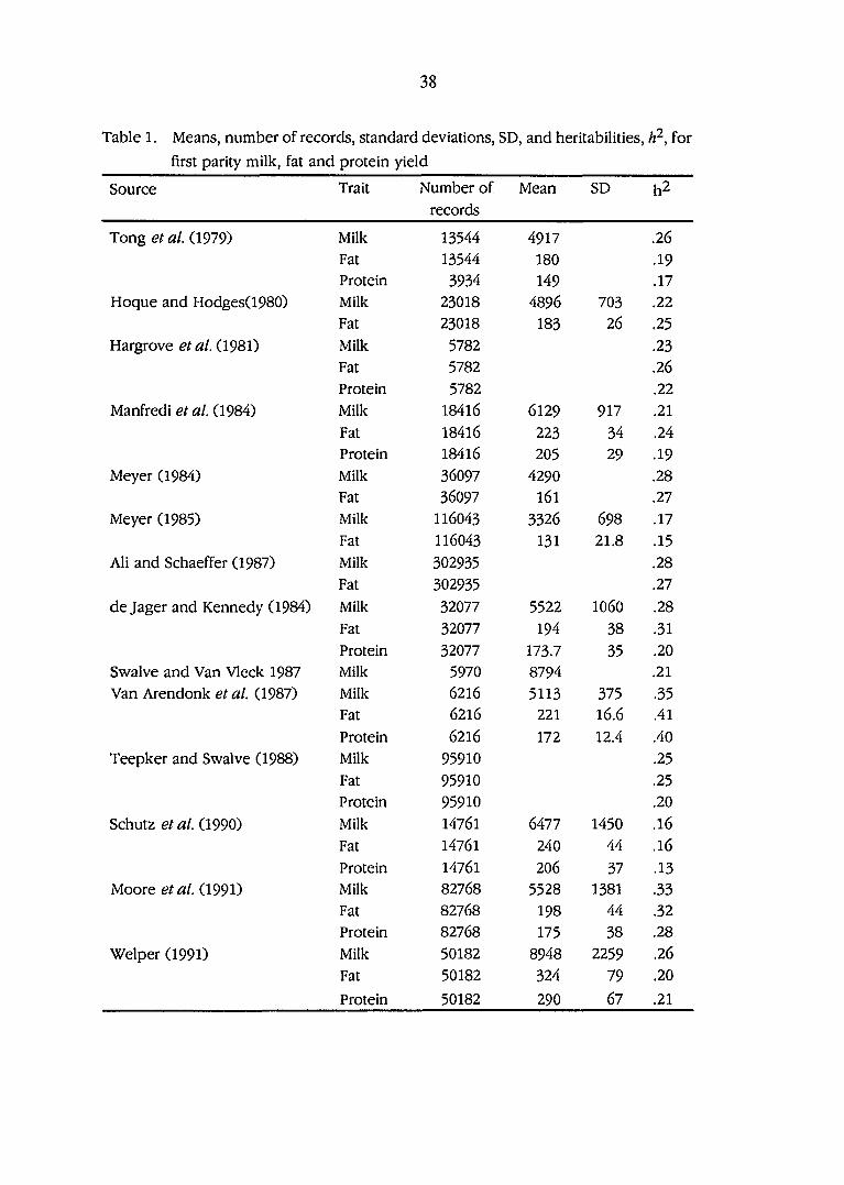
38
Table 1. Means, number of records, standard deviations, SD, and heritabilities, h^, for
first parity milk, fat and protein yield
Source Trait Number of
records
Mean SD h2
Tong et al. (1979) Milk 13544 4917 .26 Fat 13544 180 .19 Protein 3934 149 .17
Hoque and Hodges(1980) Milk 23018 4896 703 .22 Fat 23018 183 26 .25
Hargrove et al. (1981) Milk 5782 .23 Fat 5782 .26 Protein 5782 .22
Manfredi et al. (1984) Milk 18416 6129 917 .21
Fat 18416 223 34 .24 Protein 18416 205 29 .19
Meyer (1984) Milk 36097 4290 .28 Fat 36097 161 .27
Meyer (1985) Milk 116043 3326 698 .17
Fat 116043 131 21.8 .15 Ali and Schaeffer (1987) Milk 302935 .28
Fat 302935 .27
de Jager and Kennedy (1984) Milk 32077 5522 1060 .28
Fat 32077 194 38 .31
Protein 32077 173.7 35 .20 Swalve and Van Vleck 1987 Milk 5970 8794 .21
Van Arendonk et al. (1987) Milk 6216 5113 375 .35 Fat 6216 221 1&6 .41
Protein 6216 172 12.4 .40 Teepker and Swalve (1988) Milk 95910 .25
Fat 95910 .25 Protein 95910 .20
Schutz et al. (1990) Milk 14761 6477 1450 .16
Fat 14761 240 44 .16
Protein 14761 206 37 .13 Moore et al. (1991) Milk 82768 5528 1381 .33
Fat 82768 198 44 .32 Protein 82768 175 38 .28
Welper (1991) Milk 50182 8948 2259 .26
Fat 50182 324 79 .20
Protein 50182 290 67 .21

39
Table 2. Genetic and phenotypic correlations between individual production traits for first
parity
Source Trait 1 Trait 2 Number of Genetic Phenotypic
records correlation correlation
Hoque and Hodges (1980) Milk Fat 23018 .49 .82
Hargrove etal. (1981) Milk Fat 5782 .40 .78
Milk Protein 5782 .83 .94
Fat Protein 5782 .69 .84
Manfredi et al. (1984) Milk Fat 18416 .43 .73
Milk Protein 8747 .79 .90
Fat Protein 8747 .80 .80
Meyer (1985) Milk Fat 116043 .76 .90
Milk Protein 116043 .91 .95
Fat Protein 116043 .71 .91
Ali and Schaeffer (1987) Milk Fat 302935 .54
de Jager and Kennedy (1987) Milk Fat 32077 .57 .74
Milk Protein 32077 .82 .90
Fat Protein 32077 .66 .80
Teepker and Swalve (1987) Milk Fat 95910 .54 .78
Milk Protein 95910 .83 .91
Fat Protein 95910 .65 .81
Schutz et al. (1990) Milk Fat 14761 .23 .68
Milk Protein 14761 .56 .88
Fat Protein 14761 .63 .77
Moore et al. (1991) Milk Fat 82768 .61 .78
Milk Protein 82768 .86 .92
Fat Protein 82768 .71 .84
Welper (1991) Milk Fat 50182 .70 .82
Milk Protein 50182 .92 .95
Fat Protein 50182 .78 .85
of 0.20. The genetic correlations between measures of mastitis and somatic cell count reported
in the literature have been positive and of moderate magnitude, on average (Emanuelson etal.,
1988; Coffey etal., 1985). Declines in milk yield with increases in somatic cell concentration have

40
Table 3. Repeatability estimates for milk production (from Welper,
1991)
Trait Number of Records Repeatability
Milk 78163 .455
Fat 78163 .382
Protein 78163 .419
been reported by Raubertas and Shook (1982) and Bartlett et al. (1990). For the estimation of
genetic and phenotypic parameters the somatic cell count concentration (SCC, number per 10"
^ 1) is transformed to a logarithmic base. The logarithmic transformation has been shown to
reduce the heterogeneity and improve the normality of the data (Ali and Shook, 1979). Two
logarithmic transformations are common in the literature:
1) Log somatic cell count (LNSC) is logg(SCC), and
2) Somatic cell score (SCS) is log2(SCS/100)+3.
The somatic cell score rounded to the nearest integer and reported on a 1 to 9 scale (Shook,
1982; Sechrist, 1985). This review will concentrate on SCS. SCS is the measure reported by Dairy
Herd Improvement Association (DHIA) and reports by Dabdoub and Shook (1984) and Bartlett
Table 4. Means, number of records, standard deviations, SD, and heritabilities, h~, for somatic
cell score
Source Parity Number of
records
Mean SD h2
Coffey et al. (1985) 1 8659 .09
2 6122 .10
3+ 10217 .29
Banos and Shook (1990) 1 80069 2.66 1.09 .13
2 56677 2.83 1.16 .11
3+ 39362 3.15 1.17 .10
Schutz et al. (1990) 1 14761 3.07 1.21 .10
2 7806 3.34 1.27 .13
3+ 12617 3.98 1.30 .12
Welper (1991) 1 5246 2.85 .16
All 7496 2.94 .13

41
Table 5. Genetic and phenotypic correlations between production traits and somatic cell
score surveyed from the literature
Source Trait Parity Number of
records
Genetic
correlation
Phenotypic
correlation
Banos and Shook (1990) Milk 1 80069 .24 -.05
Milk 2 56677 -.17 -.16
Milk 3+ 39362 -.12 -.16
Schutz etal. (1990) Milk 1 14761 .13 -.07
Milk 2 7806 -.21 -.13
Milk 3+ 12617 -.06 -.17
Fat 1 14761 .13 -.09
Fat 2 7806 -.31 -.16
Fat 3+ 12617 -.19 -.20
Protein 1 14761 .29 -.04
Protein 2 7806 -.14 -.10
Protein 3+ 12617 .09 -.13
Welper (1991) Milk 1 5246 .15 -.04
Fat 1 5246 .12 -.07
Protein 1 5246 .18 -.04
et al. (1990) have quantified the loss in milk production from increases in SCS that will be
important in determining the economic value of somatic cell count genetic gain. The genetic
and phenotypic estimates for LNSC are consistent in direction and magnitude with recent
estimates for SCS (Monardes etal, 1983; Cue etal., 1987; Emanuelson etal., 1988). A summary
of means, standard deviations and heritabilities for SCS from the literature is given in Table 4.
Table 5 gives a summary of genetic and phenotypic correlations with milk, fat and protein, yields.
These estimates are consistent with genetic and phenotypic correlations estimated for mastitis
susceptibility and milk yield (Gonyon et al., 1982; Kennedy et al., 1982). In general, genetic
correlations between SCS and milk, fat and protein yield in later lactations were found to be
negative. Schutz et al. (1990) suggest that exposure to mastitis in the first parity might cause
deterioration in milk production in later lactations, which would account for the change in
direction of the genetic correlations. For this reason average heritabilities and correlations are
computed from parity 1 estimates only. Welper (1991) estimated a repeatability for SCS of 0.27.
This result is consistent with repeatabilities estimated for LNSCC by Monardes and Hayes (1985)
which ranged from 0.13 to 0.40.

42
Table 6. Means, number of records, standard deviations, SD, and heritabilities,
h^, for days open
Source Parity Number of
records
Mean SD h2
Kragelund et al. (1979) All 4539 100 51 .06
Berger et al. (1981) 1 72187 135 77 .02
2 72187 136 76 .03
3+ 72187 148 81 .05
Hansen et al. (1983a) 1 47710 98 35 .01
2 31162 97 35 .01
3 22389 99 35 .01
Seykora and McDaniel (1983) 1 4819 .05
Jansen (1987) 1 14951 98 42 .03
2 11996 93 38 .02
3 9039 92 39 .07
Van Arendonk et al. (1989) 1 5764 95 34 .01
2 4480 94 46 .01
3 3187 93 38 .03
Moore et al. (1991) 1 63643 101 46 .04
Fertility
Reproduction efficiency in dairy cattle is considered to be of economic importance. Breeding
efficiency is measured as services per conception, days open, days from parturition to first
breeding and similar measures (Freeman, 1976). These measures are highly related (Vinson,
1982) and largely influenced by management practices. In dairy herds it is necessary to have
cows calving at regular intervals in desirable seasons. There have been several reviews on
genetic aspects of fertility in dairy cattle (Maijala, 1976; Philipsson, 1981; Freeman, 1984;
Freeman, 1986;Janson, 1985). It is well known that a number of reproductive measures of female
fertility can show considerable genetic variation (Maijala, 1964), but the heritabilities are low,
usually ranging from 1 to 5%. It is thought that the low heritability estimates may be due to,
reduced genetic variation occurring from natural selection, or, non-additive genetic effects
(Philipsson, 1981). This review will concentrate on genetic and phenotypic estimates for one
measure of reproductive efficiency, namely, days open. This trait can be considered as a
combination of days between parturition and first insemination and conception rate.

43
Table 7. Repeatability estimates for days open
Source Parities Number of Repeatability
records
Hansen et al. (1983a) 1 - 2 56869 .10
2 - 3 34296 .13
1 - 3 34188 .08
Jansen (1987) 1- 2 6307 .06
2 - 3 4985 .07
1 - 3 2796 .23
A summary of means, standard deviations and heritabilities for days open from the literature
is given in Table 6. Hansen etal. (1983a) reported repeatabilities for days open between adjacent
parities that ranged from 0.05 to 0.14. Similar results have been reported byjansen etal. (1987).
These estimates are summarized in Table 7. In recent years a number of studies have investigated
the relationship between production and reproduction. The measures appear to be greatly
Table 8. Genetic and phenotypic correlations between production and days open
Source Trait Parity Number of Genetic Phenotypic
records correlation correlation
Hansen et al. (1983b) Milk 1 47710 .37 .25
2 31162 .43 .29
3 22389 .39 .29
Seykora and McDaniel (1983) Milk All 4819 .54 .24
Fat All 4819 .44 .24
Van Arendonk et al. (1987) Milk 1 5764 .64 .17
2 4480 .65 .16
3 3187 .27 .16
Fat 1 5764 .95 .19
2 4480 .76 .13
3 3187 .61 .18
Protein 1 5764 1.02 .19
2 4480 .48 .15
3 3187 .58 .19

44
dependent on the measure of production used. The genetic and phenotypic correlations
increase with the length of lactation over which the production is accrued (Philipsson, 1981;
Hansen et ai, 1983b). Although some results from the literature are conflicting, in general, the
relationship between days open and milk yield appears antagonistic (Freeman, 1984). Table 8
gives a summary of genetic and phenotypic correlations with 305 day milk, fat and protein,
yields.
Linear type and liveweight
Linear type traits scoring replaced categorical type traits scoring in the Holstein Friesian
breed in the United States on January 1,1983, (Lawstuen etal., 1988). Thompson etal., (1983)
summarized the advantages of the linear type trait scoring system. Several studies have reported
estimates for and the genetic and phenotypic relationships between pairs of type traits. Three
type traits will be reviewed, stature, udder depth and body depth. Stature is a measure of the
overall height of the cow with high score indicating very tall. Udder depth is a measure of the
depth of udder measured relative to the hocks of the cow a high score indicates extremely
shallow. Body depth is measure of the depth of rib in relation to the rest of the cow with a high
score indicating extreme depth.
Early reports estimated genetic and phenotypic parameters across different age groups of
cows with adjustment for age in the statistical model as a fixed effect —Thompson et al. (1980,
1981 and 1985). Recent reports have estimated these parameters within age groups — Meyer
et al. (1987) and Lawstuen et al. (1988). While Foster et al. (1988) and Boldman et al. (1992)
analyzed first parity records. In all studies reviewed, a 50 point range of scoring was used with
the exception of Schaeffer etal. (1985) and Meyer etal. (1987) where the range was 9 points.
Although, Meyer et al. (1987) analyzed British Holstein Friesian, this study is included in this
review because this is the only report that provides measures of the genetic and phenotypic
relationship between type and production traits. A summary of means, standard deviations and
heritabilities for three type traits from the literature is given in Table 9. Recent genetic
correlations have ranged from -0.22 to 0.65,0.29 to 0.41, and -0.39 to 0.80 between stature and
body depth, stature and udder depth, and udder depth and body depth, respectively. Similar
trends were observed for the phenotypic correlations but they were of lower magnitude. Table
10 summarizes genetic and phenotypic correlations between stature, body depth and udder
depth.
Meyer etal. (1987) is the only study to report genetic and phenotypic correlations between
milk production traits and linearly scored type traits. The weighted average of genetic and
phenotypic correlations across parity 1 and 2 between stature and milk, fat and protein were
of small magnitude close to zero — all phenotypic correlations were less than 0.10 and genetic
correlations less than 0.03 in absolute value. The weighted average of genetic correlations across
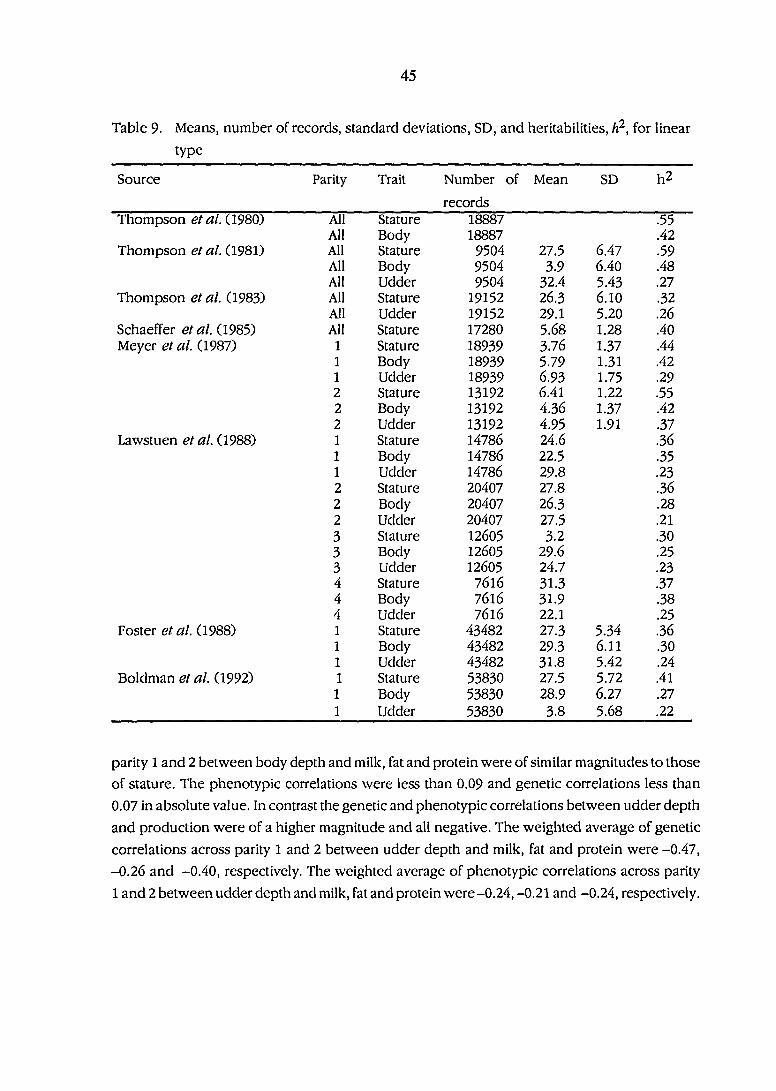
45
Table 9. Means, number of records, standard deviations, SD, and heritabilities, h^, for linear
type
Source Parity Trait Number of
records
Mean SD h2
Thompson et al. (1980) AH Stature 18887 .55 Ail Body 18887 .42
Thompson et al. (1981) Ail Stature 9504 27.5 6.47 .59 Ail Body 9504 3.9 6.40 .48 AU Udder 9504 32 j 5^3 .27
Thompson et al. (1983) AU Stature 19152 2&3 6.10 .32 AU Udder 19152 29.1 5.20 .26
Schaeffer et al. (1985) AU Stature 17280 5.68 1.28 .40 Meyer et al. (1987) 1 Stature 18939 3.76 1.37 .44
1 Body 18939 5.79 1.31 .42 1 Udder 18939 &93 1.75 .29 2 Stature 13192 6.41 1.22 .55 2 Body 13192 436 1.37 .42 2 Udder 13192 4.95 1.91 .37
Lawstuen et al. (1988) 1 Stature 14786 24^ 36 1 Body 14786 22.5 .35 1 Udder 14786 29.8 .23 2 Stature 20407 27.8 .36 2 Body 20407 26.3 .28 2 Udder 20407 27.5 .21 3 Stature 12605 3.2 .30 3 Body 12605 2^6 .25 3 Udder 12605 24.7 .23 4 Stature 7616 31.3 .37 4 Body 7616 31.9 .38 4 Udder 7616 22.1 .25
Foster et al. (1988) 1 Stature 43482 27.3 534 .36 1 Body 43482 293 6.11 .30 1 Udder 43482 31.8 5.42 .24
Boldman et al. (1992) 1 Stature 53830 27.5 5.72 .41 1 Body 53830 28.9 6.27 .27 1 Udder 53830 3.8 5.68 .22
parity 1 and 2 between body depth and milk, fat and protein were of similar magnitudes to those
of stature. The phenotypic correlations were less than 0.09 and genetic correlations less than
0.07 in absolute value. In contrast the genetic and phenotypic correlations between udder depth
and production were of a higher magnitude and all negative. The weighted average of genetic
correlations across parity 1 and 2 between udder depth and milk, fat and protein were -0.47,
-0.26 and -0.40, respectively. The weighted average of phenotypic correlations across parity
1 and 2 between udder depth and milk, fat and protein were-0.24, -0.21 and -0.24, respectively.

46
Table 10. Genetic and phenotypic correlations between linear type traits
Source Trait 1 Trait 2 Number of Genetic Phenotypic
records correlation correlation
Thompson et al. (1980) Stature Body 18887 -.09 .07
Thompson et al. (1981) Stature Body 9504 -.22 .02
Stature Udder 9504 .41 .11
Udder Body 9504 -.37 .28
Thompson et al. (1983) Stature Udder 19152 .36 .16
Meyers et al. (1987) Stature Body 18939 .65 .16
Stature Udder 18939 .27 .15
Udder Body 18939 .08 -.10
Stature Body 13192 .58 .42
Stature Udder 13192 .29 .18
Udder Body 13192 -.15 -.10
Foster et al. (1988) Stature Body 43482 .08 .14
Stature Udder 43482 .37 .16
Udder Body 43482 -.39 -.20
Lawstuen et al. (1988) Stature Body 14786 .78 .62
Stature Udder 14786 .29 .16
Udder Body 14786 -.10 -.03
Boldman et al. (1992) Stature Body 53830 .11 .14
Stature Udder 53830 .41 .16
Udder Body 53830 -.35 -.20
Table 11. Means, number of records, standard deviations, SD, and heritabilities,
h", for liveweight
Source Parity Number of Mean SD
records
Miller et al. (1981) 1 503 533 45 .57
Badinga et al. (1985) AU 2263 587 49 .25
Lin et al. (1985) 1 994 462 51 .28
Moore et al. (1991) 1 112371 504 86 .18

47
Table 12. Genetic and phenotypic correlations between production and liveweight
Source Trait 1 Trait 2 Number of Genetic Phenotypic
records correlation correlation
Miller etal 1981 Milk Liveweight 503 .51
Fat Liveweight 503 .47
Protein Liveweight 503 .45
Lin etal 1983 Milk Liveweight 994 .76 .72
Fat Liveweight 994 .84 .60
Protein Liveweight 994 .48 .60
Moore et al 1991 Milk Liveweight 82768 -.22 .11
Fat Liveweight 82768 -.27 .12
Protein Liveweight 82768 -.18 .14
Very similar genetic correlations between the three type traits and milk, fat and protein have been
found for North American Holstein (Law!or unpubl., 1991).
Miller et al. (1981) summarized results from the literature for the heritability of liveweight
in dairy cattle. Recent studies by Badinga et at. (1985), Lin etal. (1985) and Moore etal. (1990
and 1991) have reported estimates for Holstein dairy cattle. A summary of means, standard
deviations and heritabilities from these studies is given in Table 11. A cow's liveweight is
determined by her genotype, age and environmental conditions. Several studies have suggested
larger cows produce greater milk yield (Miller and McGillard, 1959; Clark and Touchberry, 1962;
Harville and Henderson, 1966). The phenotypic correlations reviewed support these observa
tions. Tlie genetic correlations were inconsistent, the studies using records from experimental
herds (Miller et al., 1981; Lin et al., 1985) reported large positive genetic correlations, whereas,
studies using large numbers of field records (Badinga etal, 1985; Moore etal, 1991) reported
low negative genetic correlations. A summary of genetic and phenotypic correlations between
production traits and liveweight is given in Table 12. Repeatability of 0.53 for liveweight has been
reported by Badinga et al (1985). Moore et al (1991) also reported genetic and phenotypic
correlations between liveweight and days open of -0.17 and -0.10, respectively.
48
PAPER 1. PREDICTION OF RESPONSE WITH OVERLAPPING
GENERATIONS ACCOUNTING FOR MULTISTAGE SELECTION
Summary
A generalization of Hill's equations predicting response to selection is developed that
accounts for multiple stage selection in either or both sexes. The method accounts for the flow
of genes for animals selected at later stages. This allows for the use of genetic gains from later
stages, which explain the reduction in variance due to previous selection. Genetic gains from
different selection differentials in each reproductive pathway are incorporated into the
equations. The asymptotic response to a single cycle of selection is shown to agree with classical
selection theory.
The method is applied to a dairy progeny testing scheme representative of an artificial
insemination organization in the USA. Two models were compared 1) the first accounted for
two stage selection of males, the first stage was based on pedigree information and whose
second stage on both pedigree and progeny test information and 2) the second model assumed
single stage male selection. Selection was based on milk volume, fat and milk protein yields.
The predicted asymptotic rates to a single cycle of selection were overestimated by 6% and the
cumulative response to continuous selection over 20 years was overestimated by 8% when single
stage male selection was assumed.
Keywords: iVIultistage selection. Response, Overlapping generations. Dairy cattle
Introduction
With discrete generations, selected individuals are mated at approximately the same time. The
generation interval is the interval between matings in successive generations, or when
replacements for the next generation are born. When generations overlap, the replacement of
parents by selected offspring approaches a continuous process. The generation interval in a
population with overlapping generations can be calculated as the average age of parents at the
birth of their selected offspring. The original formulae for predicting the rates of response to
selection in overlapping generations were obtained by Dickerson and Hazel (1944) and
generalized by Rendel and Robertson (1950). In addition to identifying the intensities of
selection and changes in genetic variation due to two stage selection Dickerson and Hazel (1944)
distinguished between selection in the male and female populations. The rate of response to
selection in a continuing breeding program essentially equals the ratio of the mean selection
intensity of the parents to the mean age of parents when progeny are born.
49
A number of authors have computed predictions of response to selection before the
asymptotic rates have been reached. Searle (1961) examined the improvement in genetic gain
from the use of herd testing and artificial insemination (AI). Alternative methods were described
by Brascamp (1973), McClintock and Cunningham (1974), and Hill (1974). The methods are of
two kinds. The first, attributed to McClintock and Cunningham (1974), considers the number,
genetic contribution (1/2 to progeny, 1/4 to grand progeny, etc.), and the year of birth of
descendants derived from an insemination by a single male. The total number of expressions
of an individual genotype up to a specified time is computed. These expressions can be
discounted. This method is useful when considering the dissemination of genes from a single
animal. The second formulation considers the change in the mean breeding value of each age
group in the population. Hill (1974) and Elsen and Mocquot (1974) independently described
a matrix method for modeling the response to selection with overlapping generations. Several
simplifying assumptions were made, most of which were reasonable, for computing the
response to selection from artificial selection programs in large domestic species. The
heritabilities and genetic correlations were assumed unchanged, and thus the phenotypic and
genotypic selection differentials remained constant over time. Single stage selection was
assumed in both sexes. Dentine and McDaniel (1987) used a matrix approach to compute short
term genetic gain for milk yield, for USA. The method was deterministic and based on the
methods of Hill (1974). Ducrocq and Quaas (1988) described a method for optimizing truncation
selection across distributions as well as an application of this procedure utilizing the matrix
methods of Hill (1974) in dairy AI breeding plans. These approaches have assumed a single stage
of selection occurs within the population. If multiple stage selection is not taken into account
then these methods may overestimate the selection response. The purpose of this paper is
outline a procedure which can be used when multistage selection occurs.
Prediction of response with overlapping generations
This discussion will use Hill's (1974) matrix notation. An iterative process can be used to
compute the proportion of genes at timer that were derived from animals at time 0. Assume those
h male age groups and k female age groups are present in the population. The equation is then
(Hill, 1974; Eq. 2):
m, =Pm,_i [1]
where P is an ih+k) by (/»+/:) matrix corresponding to the paths of gene transmission via
reproduction and aging, is an ih+k) x 1 column vector, with element m,(() being the
proportion of genes, in males of age / (/ < h) in year t, or in females of age i - h (/ > /j) in year
t, originating from males in year 0. A similar equation to Eq. 1 can be derived for the genes
originating from females in year 0 in animals in born year t by substituting f, for m, in Eq. 1

50
Because an animal has all of its own genes at time f = 0, the vectors fg and iiiq are defined broadly
as:
fo=[Ou 1 Oi./,_i] and nio = [l
The blocks of P correspond to the pathways of genes;
' males to males | females to males ' — ^ males to females [ females to females
The resulting structure of P is:
Pu • ••• P{,h Plh+\ • ••• Plh+k 1 0 •• ... Q 0 • ••• 0 0 1 : : ;
0 0 •• • 1 0 0 • ••• 0 Ph+u • P/I+l./I Ph+\,h+l • "• Ph+lMk
0 ... 0 1 0 •• • ••• 0 : I 0 1 :
0 ... 0 0 0 •• • 1 0
The matrix P combines information on reproduction and aging. Tlie tth element of the first row
refers to proportion of genes transferred to males (/ < A) or to females Q > K) in year t from males
of age / in year t-1. Similarly, The /th element of the h+1 row refers to proportion of genes
t r a n s f e r r e d t o m a l e s ( / < h ) o r t o f e m a l e s ( / > h ) i n y e a r t f r o m f e m a l e s o f a g e i i n y e a r t - 1 .
The response to selection is the contribution of genes by reproduction alone. To remove the
contribution of genes by aging a matrix Q is defined from P by setting the elements of rows 1
and /i + i of P to zero.
The response in year t to one cycle of selection occurring at year 1 is (Hill, 1974; Eq. 5):
'/=CP*-Q^Cmogm+fo5/>' [2]
where and iyare the genetic gains from male and female selection respectively. The genetic
gain vector s can be defined as:
s = Cmogw+fog/) [3]

51
Equation [2] assumes that the same females and males are used to breed replacements for
both sexes. This is not normally the case in dairy cattle AI programs. Two additional matrices
are required to specify the passage of genes by reproduction to males only (Em) and the passage
of genes by reproduction to females only (Ef). These two matrices of dimensions ih+k) by ih+K)
are formed from:
and;
-•Ir respectively. To compute the response to selection, a genetic gain vector for each sex, for
male and s/ for females, needs to be defined as:
~ (^oSmnt fm )
S f = ( m Q g „ t f + Î Q g f f )
where gi is the genetic gain for the ith pathway. The response to selection in the first time period
is:
i\ = Ems„, + Efsy ^ [61
and, in general for t >1 (Hill, 1974; Eq. 22):
r, = + EmQ'-^s„, + EfQ'-^s y [7]
The response to continued selection, whether Eqs. [31 or [6] and [7l are used, is best computed
using:
n
f=l
Equation [8] is an approximation for response to continuous selection in the short term (less than
20 years). Because the effects of inbreeding are ignored, phenotypic and genetic (co)variances
are assumed constant over time, and the realized genetic gain is assumed to equal the expected
genetic gain. For longer periods, the effects of inbreeding depression must be considered. A
simple method that accounts for inbreeding depression is:
r,'=r,-Wi, [91
where i, is the vector of percentage inbreeding for male and female age groups at time t and
where B (A + A) hyCh + k) matrix which is the product of the regression coefficient of percentage
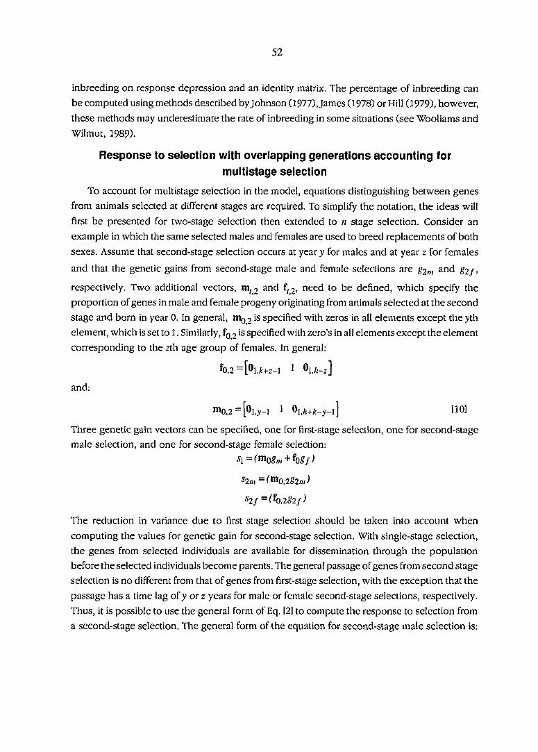
52
inbreeding on response depression and an identity matrix. The percentage of inbreeding can
be computed using methods described byjohnson (1977), James (1978) or Hill (1979), however,
these methods may underestimate the rate of inbreeding in some situations (see Wooliams and
Wilmut, 1989).
Response to selection with overlapping generations accounting for
multistage selection
To account for multistage selection in the model, equations distinguishing between genes
from animals selected at different stages are required. To simplify the notation, the ideas will
first be presented for two-stage selection then extended to n stage selection. Consider an
example in which the same selected males and females are used to breed replacements of both
sexes. Assume that second-stage selection occurs at year y for males and at year z for females
and that the genetic gains from second-stage male and female selections are g2„, and g2f,
respectively. Two additional vectors, m, 2 and f,2, need to be defined, which specify the
proportion of genes in male and female progeny originating from animals selected at the second
stage and born in year 0. In general, mQ 2 is specified with zeros in all elements except theyth
element, which is set to 1. Similarly, fg 2 is specified with zero's in all elements except the element
corresponding to the zth age group of females. In general:
*0,2 =[Ol,/fc+z-l 1 Ol,/f-z]
and:
™0,2=[Olj-l 1 110]
Three genetic gain vectors can be specified, one for first-stage selection, one for second-stage
male selection, and one for second-stage female selection:
^2m -(^0,2S2m)
•^2/ =^^0,2^2/^
The reduction in variance due to first stage selection should be taken into account when
computing the values for genetic gain for second-stage selection. With single-stage selection,
the genes from selected individuals are available for dissemination through the population
before the selected individuals become parents. The general passage of genes from second stage
selection is no different from that of genes from first-stage selection, with the exception that the
passage has a time lag of >> or z years for male or female second-stage selections, respectively.
Thus, it is possible to use the general form of Eq. [2] to compute the response to selection from
a second-stage selection. The general form of the equation for second-stage male selection is;

53
, . 2 m _ Q l - y + l t > y [ 1 1 ]
and for female second-stage selection:
r, 2/ _ /p/-z+l = rP'-^^^-Q™;52/ f>z [12]
The total response to a single cycle of selection, assuming >> > z, is an extension of Eq. [4] that
incorporates Eqs. [11] and [12];
'•/ =
( P ' - Q ' M t < z
( P ' - Q ' ) s i + ( ¥ ' - ' - Q ' - ' ^ ^ ) S 2 f t > z [13]
rP' - Q' ) S 2 f + f)S2m t > )'
when there is «-stage selection in males and Mi-stage selection in females, the general form of
Eq. [13] holds. In Eq. [13], the quantity (the response for males from second-stage selection)
is added to the first-stage selection responses for both males and females and to the second-
stage selection response for females during the year the male second-stage selection occurred.
If a third-stage selection of males had taken place, the response from this selection would be
added to the cumulative responses from preceding years for both males and females in the year
it occurred and in subsequent years. Thus, the general form of Eq. [13] for n and m stage selection
occurring at year and Cz„ < y^) in males and females, respectively, is:
CP'-Q'M t < z
( P ' t > z
/} = i(P ' - Q ' f P ' - ) '+^-t>y [14]
The same principles are used to define the response to selection for multistage selection
when different selection intensities are used to breed replacements for each sex. The only
difference is the need extend for the four different genetic gain vectors, namely, S2„,y, s^,,
and S2ff, in the case of two-stage selection, where;
^Imm =(^0,28lmm)
Slmf =(^Q.282fin)
^ 2 f f = ( h 2 8 2 f f )

54
where simni'^lmf ^Iff correspond to the genetic gain from second stage selection for
each of the four reproductive pathways. The response to selection from stage two can be defined
directly from the single stage Eqs. [4] and [5], allowing for the time lag between stage 1 and stage
2 selections and for the appropriate genetic gain vectors. The response to the second stage male
selection is:
ri^"'=Ems„,„, + Efs„,f t = y
r?"' = P/-,lT + + EfQ'-^s„,y t > y [15]
with the selection occurring at yearj. Similar equations can be derived for second-stage female
selection by replacing y (the year second stage female selection occurs) with z, s^with S2w^and
^2fm with ^2nmv total response to a single cycle of selection, assuming two-stage selection
only, is:
^ r j \ < t < z r, = r , + r f ^ z > t < y [16]
r , + + r f " * y > t
where r} is the response to selection from stage one in year t. Equation [16] can easily be
extended to n stage selection. Assume that male selection occurs after female selection for each
stage, with stage t occurring at years z, and y, and with n stage occurring in years tj and p for
females and males, respectively. Then the response to selection is:
ft =•{
r , + r y
r, + + /•/ 2m
1 < / < Z2
Z 2 < t < y 2
y 2 ^ t < z ^ [17]
r, -h t-y + rf"' + i-y + rj"'+,---,+rf pm yp ^ t < z „
To compute the cumulative response from n multiple stage selection Eqs. [15] or [17] are used
in Eq. [8]. It has been assumed that the elements of Pare constant over time. Ducrocq and Quaas
(1988) suggest taking into account the genetic merit of different age groups when deriving the
elements of P. This results in a P matrix which varies over time. The equations derived here can
easily account for a P matrix which varies with time. Extensions to Eqs. [14] and [15] are given
in the Appendix.

55
Asymptotic response to selection
The total response achievable from a single cycle of selection, using the equations
developed in the previous sections, can be shown to agree with the methods of Dickerson and
Hazel (1944) and Rendel and Robertson (1950), which are commonly used. To compute the
asymptotic response, the limit lim r, must be evaluated. Two general results are required:
//mQ'=0 [18] / —>CX3
when t exceeds h or k, and (Hill, 1974; Eqs. 9 and 11):
limP'=^ [19] /->oo 2L
where Lis the average generation interval (i.e., CL„,„, + L„,^ + Ly„, +Lj^)/4), where 1 is a vector
of I's with dimensions 1 and h+k and where visa vector of the expected gene contribution of
the ith age group. The vector v of dimension h+k, is defined from the elements of the matrix
P (Hill, 1974) as:
• h ^ ( P l j + P h + l j ) i = l , . . . , h
^ ( P i j + P h + i j ) i = h + l h + k
The asymptotic response to single-stage selection with same selected males and females
breeding replacements for both sexes is (Hill, 1974; Eq. 12):
lim r, = lim (P' -Q' )s = [20] >oo t—^oo ZL,
which is identical to Rendel and Robertson's formulation with and With
multistage selection the asymptotic response is:
t—^oo /—>00
_ Iv'CSl+,•••,+s„/+s^, J rn.i - ^
which, for two stage selection, is identical to the formulation given in Dickerson and Hazel
(1944), using and Rendel and Robertson's (1950) notation, with Gff= Gf,,, and G,„„, = Gmf-

56
Equation [21] can be written in terms of Rendel and Robertson's formula for two-stage selection
as:
, . G l , + G f + + p f G f km I't = ——
^mm ^mf ^fm [22]
/—>oo
where Gj is the expected genetic gain from the jth sex and ith stage of selection and where
Pj is the proportion of the /th sex bred from animals selected at the second stage.
When different selection differentials are used for breeders of males and females, the
asymptotic response is the same for both sexes. If v„, and vy are vectors defined as the
reproductive values of male and female breeders, respectively, these are given (Hill, 1974; Eq.
25) as:
r h
I p u j
h+k
[m
i = h + \,...,h + k
and:
r It
y=i h+k
Y^Ph+lj j=l
i —
i = h + \,...,h + k
The asymptotic response for single stage selection is (Hill, 1974; Eq. 24):
1 . Urn r, = t—^oo
VmS„,+vyS/
2L [23]
Equation [23] is identical to Rendel and Robertson's response to selection formula Extension
of this result to «-stage selection is straightforward and can be derived directly from Eq. [23], as:
lint r, = /—>oo
Vffi CS/ ? I + • • • • • + Sn,mm ) + Jhi)
2L 1. [24]

57
Table 1. Population parameters.
Number of young sires selected 70
Proportion of young sires bred to females in the population 6%
Total cow population size 300,000
Selection Intensities
1. Young sires (first stage, top 3.00%) model 1. 2.268
2. Bull dams (top 5.00%) 2.063
3. Sires of males (10 from 70) model 1. 1.553
4. Sires of females (25 from 70) model 1. 1.032
5. Sires of males (top 0.43%) model 2 2.947
6. Sires of females (top 1.00%) model 2 2.665
Average number daughters for sires, grand and maternal grand sires 500
Average number of records for bull dam's dam 5.00
Average number of records for young sires dam 1.90
Average number of daughters for progeny test of young sires 50
This can be written in the form of Dickerson and Hazel's response to two-stage selection [using
and Rendel and Robertson's (1950) notation] as:
Urn y - ^ Pninfimm + Pff^ff + Pmpmf + PfinGj„, ' ^mm + mf + + %
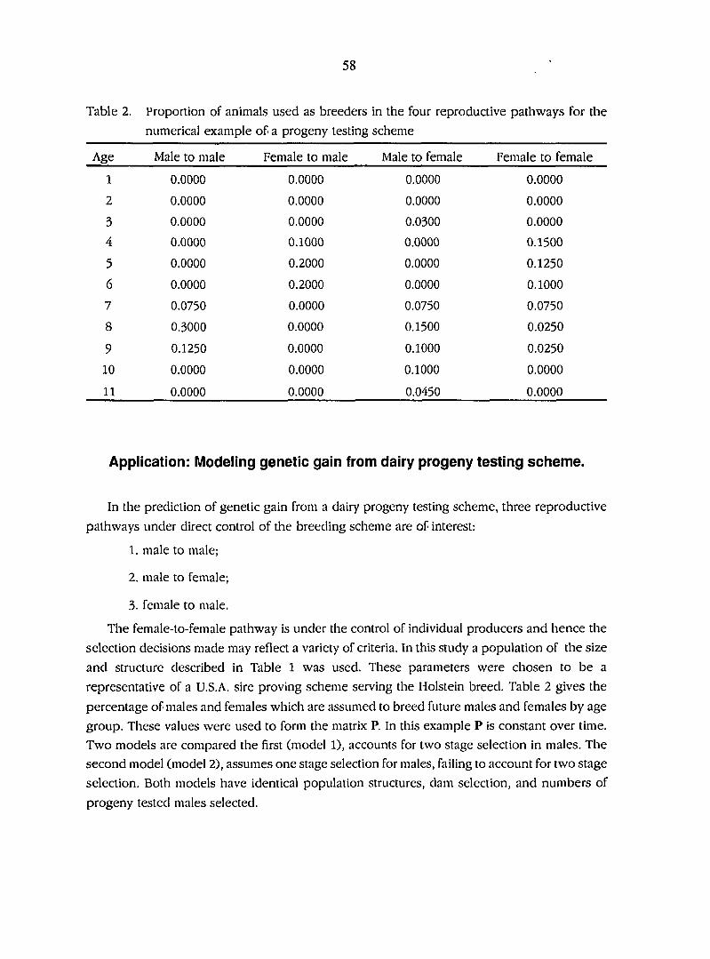
58
Table 2. Proportion of animals used as breeders in the four reproductive pathways for the
numerical example of a progeny testing scheme
Age Male to male Female to male Male to female Female to female
1 0.0000 0.0000 0.0000 0.0000
2 0.0000 0.0000 0.0000 0.0000
3 0.0000 0.0000 0.0300 0.0000
4 0.0000 0.1000 0.0000 0.1500
5 0.0000 0.2000 0.0000 0.1250
6 0.0000 0.2000 0.0000 0.1000
7 0.0750 0.0000 0.0750 0.0750
8 0.3000 0.0000 0.1500 0.0250
9 0.1250 0.0000 0.1000 0.0250
10 0.0000 0.0000 0.1000 0.0000
11 0.0000 0.0000 0.0450 0.0000
Application: Modeling genetic gain from dairy progeny testing scheme.
In the prediction of genetic gain from a dairy progeny testing scheme, three reproductive
pathways under direct control of the breeding scheme are of interest:
1. male to male;
2. male to female;
3. female to male.
The female-to-female pathway is under the control of individual producers and hence the
selection decisions made may reflect a variety of criteria. In this study a population of the size
and structure described in Table 1 was used. These parameters were chosen to be a
representative of a U.S.A. sire proving scheme serving the Holstein breed. Table 2 gives the
percentage of males and females which are assumed to breed future males and females by age
group. These values were used to form the matrix P. In this example P is constant over time.
Two models are compared the first (model 1), accounts for two stage selection in males. The
second model (model 2), assumes one stage selection for males, failing to account for two stage
selection. Both models have identical population structures, dam selection, and numbers of
progeny tested males selected.
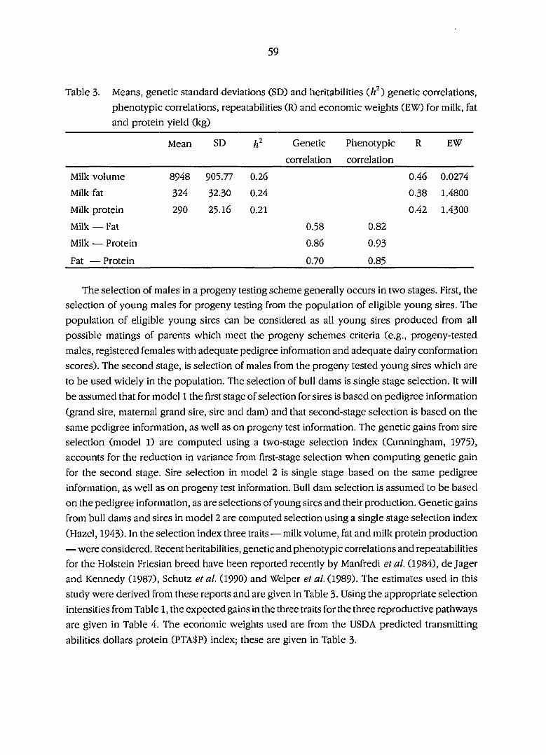
59
Table 3. Means, genetic standard deviations (SD) and heritabilities genetic correlations,
phenotypic correlations, repeatabilities (R) and economic weights (EW) for milk, fat
and protein yield (kg)
Mean SD h' Genetic
correlation
Phenotypic
correlation
R EW
Milk volume 8948 905.77 0.26 0.46 0.0274
Milk fat 324 32.30 0.24 0.38 1.4800
Milk protein 290 25.16 0.21 0.42 1.4300
Milk — Fat 0.58 0.82
Milk — Protein 0.86 0.93
Fat — Protein 0.70 0.85
The selection of males in a progeny testing scheme generally occurs in two stages. First, the
selection of young males for progeny testing from the population of eligible young sires. The
population of eligible young sires can be considered as all young sires produced from all
possible matings of parents which meet the progeny schemes criteria (e.g., progeny-tested
males, registered females with adequate pedigree information and adequate dairy conformation
scores). The second stage, is selection of males from the progeny tested young sires which are
to be used widely in the population. The selection of bull dams is single stage selection. It will
be assumed that for model 1 the first stage of selection for sires is based on pedigree information
(grand sire, maternal grand sire, sire and dam) and that second-stage selection is based on the
same pedigree information, as well as on progeny test information. The genetic gains from sire
selection (model 1) are computed using a two-stage selection index (Cunningham, 1975),
accounts for the reduction in variance from first-stage selection when computing genetic gain
for the second stage. Sire selection in model 2 is single stage based on the same pedigree
information, as well as on progeny test information. Bull dam selection is assumed to be based
on the pedigree information, as are selections of young sires and their production. Genetic gains
from bull dams and sires in model 2 are computed selection using a single stage selection index
(Hazel, 1943). In the selection index three traits — milk volume, fat and milk protein production
— were considered. Recent heritabilities, genetic and phenotypic correlations and repeatabilities
for the Holstein Friesian breed have been reported recently by Manfredi et al. (1984), dejager
and Kennedy (1987), Schutz et al. (1990) and Welper et al. (1989). The estimates used in this
study were derived from these reports and are given in Table 3. Using the appropriate selection
intensities from Table 1, the expected gains in the three traits for the three reproductive pathways
are given in Table 4. The economic weights used are from the USDA predicted transmitting
abilities dollars protein (PTA$P) index; these are given in Table 3.

60
Table 4. Genetic gain (kg) for the three traits and the asymptotic response to selection calculated
using Eq. 24
Model 1
Milk volume Milk fat Milk protein
Male to male first stage 1216.85 29.52 30.82
Male to female first stage 1216.85 2&52 30.82
Male to male second stage 972.09 22.40 23^4
Male to female second stage 735^8 16.94 17.89
Female to male first stage 1358.13 32.17 3437
Asymptotic rate 200.05 4.75
Model 2
5.00
Milk volume Milk fat Milk protein
Male to male first stage 2336.91 55.67 58.51
Male to female first stage 2140.41 5&43 52.91
Female to male first stage 1358.13 32.17 34.37
Asymptotic rate 213.91 5.06 543
To predict the response to selection over time with overlapping generations and which two
stage selection (model 1), Eq. [17] is used. More specifically, if two-stage male selection occurs
at the start of year 7 (when young sires are 6 years old), then the equations are:
/•} = Ems„, + Efs f
r j = + EmQ'~'s„, + EfQ'"^s y
r f " ' = E m s 2 „ , „ , + E f s 2 „ , / t = 7 [27]
r f " ' = P/f-i' + EinQ'-^S2„,„, + EfQ'-''s2„,/ / > 7
P, Em and Ef can be formed from Table 2. The genetic gain vectors s„,, Sy, S2„,yand S2„,„, have
dimension 22, with the following form (values for milk are from Table 4):
(1) 4 =[1216.85 Oi.,io 1216.85 Oi,io],

61
Model 2 Model 1 T3
•a
10 20 30 40 50 Year
Figure 1 Response to a single cycle of selection for protein yield
100 Model 2 Model 1
>> c
5 10 15 20 Year
Figure 2. Response to cumulative selection for protein yield
(2) 4 =[735.48 0i.,2i],
C3) 52m/;»=[0u-6 972.09 Oi^^-isj.and
C4)s'2„,f=[0ue 735.48
The response to selection for model 2 is computed using Eqs. [6] and [7], where the appropriate
genetic gains vectors are (values for milk are from Table 4):

62
Table 5. Response to a single cycle of selection for the three production traits for model 1 and
model 2 (all amounts in kg)
Model 1 Model 2
Year Milk Fat Protein Milk Fat Protein
1 0.0 0.00 0.00 0.00 0.00 0.00
2 0.0 0.00 0.00 0.00 0.00 0.00
3 3&5 0.89 0.92 64.21 1.51 1.59
4 0.0 0.00 0.00 0.00 0.00 0.00
5 0.0 0.00 0.00 0.00 0.00 0.00
6 0.0, 0.00 0.00 0.00 0.00 0.00
7 156.0 3.71 3^9 174.13 4.10 4.31
8 305.6 7.27 7j& 337.01 T93 834
9 207.0 4^3 5.17 22839 5.37 5.65
10 203.0 4^3 5.07 224.38 5J8 5.55
11 142.3 3.38 3.55 155.64 3.66 3.85
12 115.4 2.74 289 122.81 2.90 3.06
13 159.5 3.79 4.01 166.44 393 4.16
14 193.4 4.59 4^6 202.83 4.78 5.06
15 2333 5.54 5.84 248.28 5.85 6.17
16 2663 6.32 6.65 285.73 6J3 7.09
17 225.7 5.36 5.64 243.57 5J3 6.04
18 192.3 4.57 4.80 207.45 4.88 5.14
19 173.1 4.11 433 185.59 437 4.61
20 164.9 3.92 4.13 175.15 4J3 4.36
(1) a;, = [2366.91 Oi^lO 2140.41 Olalo],
(2) a}: = [735.48 0ia-2I]>
The cumulative response to continuous cycles of selection for both models is computed
using Eq. [8]. The models were run for 20 years and the results for both responses to a single
cycle of selection and cumulative responses to continuous selection for the three traits and two
models are given in Table 5.
63
The responses to selection for the three traits and both models show considerable oscillation
in the first few years before the asymptotic rate are reached. This is clearly seen in Figure 1 for
protein yield and in Table 5 for all traits. If the model 1 is allowed to run until the response from
a single cycle of selection stabilizes, the following values are obtained: 200.5, 4.75 and 5.00 for
milk, fat and protein, respectively. These values are identical to those calculated (Table 4) in the
terms of classical selection theory. Assuming single stage selection for males (model 2) the
asymptotic rates obtained are: 213.74, 5.04 and 5.31 for milk, fat and protein respectively: which
over estimate the predicted rates accounting for two stage selection by at least 6%.
The cumulative response to selection for protein yield for both models is illustrated in Figure
2. Calculating the cumulative response to selection from the model 2 rather than model 1, results
in cumulative responses for 20 years of 3022, 71 and 75 kg compared to 2774, 66 and 69 kg for
milk, fat and protein, respectively, which would over-estimate the response by at least 8% for
all traits. The extent of overestimation depends upon the nature of selection and the generation
intervals in the four reproductive pathways. Because multistage selection increases the
generation interval, which increases the degree of over-estimation from assuming single stage,
the breeding equations presented should be used to compute the response to selection. The
overestimation of response results from the failure to account for the flow of genes from animals
selected in different stages and reduction of variance caused by prior selection in the estimation
of genetic gains. The methods of Cunningham (1975) used here to compute genetic gains for
two-stage sire selection are only valid for two stages of selection. After two stages of selection,
the distribution of selected individuals is no longer normal. For situations where selection
involves more than two stages the effect of the departure from normality on the computation
of genetic gains from later stages will require consideration when applying the breeding
equations.
Appendix
Equations [14] and [15] are presented assuming P is constant over time. In situations where
P is known a priori to vary with time or truncation selection across distributions of individuals
is applied (see Durcoq and Quaas, 1988) the a simple extension to these equations can be used.
Define P*' as:
P*' =P, XP,_IX,...,XPI [Al]
where P/ is the P matrix at time t. The extension to Eq. [14] is:

64
C P ^ ' - Q ' M t < z
(P*' - Q' - Q'-:+l )s2f t > z
/; = •( fp*' - Q' f )S2 f+rp*'"^""^ - j,2m f ^ y [A2]
/P*' )Snm t>y^
The extension to Eq. [15] requires P, Em and Ef to be indexed in time:
/f'" = Ein,s^,„,+Ef,s„,/ t = y
rr"' = P,/ilT + Ein,Q'-^s„,„, + Ef,Q'-^s„,y. / > y
Equations [A2] and [A3] can be substituted for Eqs. [14] and [15] and used in Eqs. [17] and
[8].

65
PAPER 2. ECONOMIC VALUE OF RESPONSE FROM SIRE SELECTION IN DAIRY CATTLE—A LINEAR PROGRAMMING
MODEL
Abstract
A linear programming model that accounts for the economic consequences of response to
selection to the producer enterprise over a given planning horizon is described. A procedure
is given in detail for defining upper and lower bounds constraints on variables that are correlated
in the linear programming model. This procedure enabled the linear programming model to
construct a feasible hyperspace that reflects the relationship between the variables in terms of
the trend in the relationship and the variation around this trend. The linear programming model
was used to compute optimal rates of response to selection for four planning horizons. The
optimal response to selection per year for the production traits was closest to the maximums
achievable from a gene-flow model. Of all the non-production traits, days open had the greatest
proportion of its maximum achievable from a gene-flow model. The linear programming model
was used to compute relative economic weights (REV) for the nine traits for each planning
horizon. The REVs for milk, fat, and protein production were considerably larger than the REVs
for the non-production traits for all planning horizons. Somatic cell score had the largest REVs
of the non-production traits in all planning horizons.
Introduction
Definition of the breeding objective is the first requirement for development of a selection
program. Selection for multiple traits requires that the breeding objective define the relative
merits of each trait under selection. Selection of livestock is an investment for which the future
benefits accrue from the descendents of the selected group. The first consideration in defining
the breeding objective is to decide who should benefit from the genetic improvement. Different
segments of the industry may have conflicting goals (Miller and Pearson, 1979). The choices of
the breeding objectives are dependent on the level of system being modelled—national, farm
enterprise or animal level. In the case of the dairy industry, artificial insemination organizations
are selling technological change to producers, primarily semen from highly selected sires. The
adoption of genetic improvement constitutes a continuous process of technological change that
affects net income of producers throughout the life of their farm business. Therefore, the
development of selection objectives that maximize net income to producers will be beneficial
to both producers and artificial insemination (AI) organizations. The benefit to AI organizations,
both cooperative and private, will result from providing a superior product that should aid in
increasing the total number of cows bred artificially; hence, modeling at the producer level can
66
define breeding objectives beneficial to both producers and AI organizations.
Literature review
The definition of a profit function has been the first step in determining the economic value
of a number of traits. Profit functions have generally been concerned with formulating a function
representing the producer enterprise—labor, capital, housing, feeding, production, and
reproduction. This function is then used to determine the profitability on an individual animal
basis or on an individual animal per unit time basis. The profit per animal or profit per animal
per unit time can be used as a selection criterion or used in a selection index approach to derive
economic weights (Norman and Dickerson, 1971). Andrus and McGillard (1975) advocated the
use of the profit function over selection index when the genetic correlations among traits are
unknown. Gill and Allaire (1976a, b) developed a lifetime profit equation for dairy cattle. The
lifetime economic merit for a cow was computed from the cow's production, reproduction and
liveweight traits and expressed as profit per day of herd life. It was shown that the heritability
of profit per day of herd life was greater than various milk yield expressions. Lin and Allaire
(1977,1978) used a profit function to directly develop a pseudo selection index. The aggregate
genotype was equated to profit per animal per unit time. Lin and Allaire (1977,1978) used a profit
function based on first lactation information to predict long-term profitability. Balaine et al.
(1981) extended the work of Lin and Allaire (1977,1978) by considering the repeatability of net
profitability measures. They found that the repeatability of total profit, profit per day of herd life,
and profit per unit investment was approximately 0.4, 0.3, and 0.3, respectively. The
repeatabilities of profitability measures were lower than for production traits.
If the breeding objective is to maximize the economic benefits of genetically improved
livestock to the producer, then the use of a profit function as the selection criterion has several
limitations. When relative changes in the prices and costs occur, genetic and phenotypic
variances and covariances would require re-estimation (Pearson and Miller, 1979). Dairy sire
selection is most efficient when selection is based on first lactation information. Because the
repeatability of profit functions is low (Balaine etal., 1981), there could be increased inaccuracy
in meeting the breeding objective. The profit function only considers the profit from the lifetime
of an individual cow, which does not consider the cumulative effect of the flow of genes over
time. The use of profit per day of herd life fails to account for differences in herd life and the
economic value of these differences over the producer's planning horizon.
An alternative approach is to use selection index procedures that use economic weights to
determine the relative merit of different traits. Selection index procedures have been reviewed
by Lin (1978). There have been several reports of economic selection indices for dairy cattle,
most of which have been concerned with economic values for milk components. The reported
selection indices fall into two categories (Gibson, 1987): omitting the costs of production (thus

67
overestimating the economic values of the traits), or including the costs. Hazel (1956)
emphasized that the economic weight should reflect the net profit to the enterprise that accrues
from a unit change in a trait and that this value should not include net profit accruing from
changes in correlated traits.
Brascamp et al. (1985) used the concept of normal profit to show that economic weights
derived from a profit function describing different economic perspectives were equivalent. The
concept of normal profit is based on the theory of competitive equilibrium of firms. The theory
relies upon having a large number of producers producing a homogeneous product in a market
that allows free entry at any time. The long-term real profit (normal profit) for all producers is
zero since the operating profit is considered a cost of production. Smith etal. (1986) stated that
these conditions underline the concept that the change in net income from genetic improvement
comes from reducing the cost of production per unit of output, not from increases in enterprise
scale nor from improvement of management practices.
Gibson (1989a) discussed methods for deriving economic weights for milk components
using the Canadian milk market as an example. The procedure suggested was developed for
situations in which output restrictions exist in the market place and incorporated the concepts
of rescaling discussed by Smith etal. (1986). The economic weights were derived as the change
in profit resulting from a change in yield. Gibson (1989b) noted that, in a free market (no output
restrictions), the rescaling was not required. The economic weights were found to vary widely,
depending on whether a restricted or a free market was assumed.
The methods reviewed for the derivation of economic weights have largely equated the
marginal economic value of unit product improvement with the varying complexity of the
economic models. The economic weights derived have been concerned with productive traits,
whereas little or no work has been reported on the development of economic weights for non
productive traits. These methods have not accounted for the flow of genetic improvement from
sire selection through the producer herd over time. A one-unit increase in a product due to
genetic gain will affect the levels of genetic gain achieved for other correlated traits, and these
changes must be considered simultaneously when evaluating the economic worth of that one
unit change. The studies reviewed did not consider the economic consequences of selection on
correlated traits of economic importance. Such indirect selection will affect the future net income
of the enterprise and the ultimate value of the accrued genetic gain for all traits being selected.
A model that accounts for the flow of genetic improvement in productive and non-productive
traits over time is required. James (1982) notes that the purpose of economic weights is to
maximize profit. Similarly, Gibson (1987) states that animal breeders should use economic
selection indices to optimize the genetic improvement of the economic merit of dairy cattle. If
the breeding goal is to maximize a function of net income of the dairy enterprise then a key
question is—what is the economic contribution of unit genetic improvements in productive and

68
non-productive traits to the accrued producer net income?
Jansen and Wilton (1984) have discussed the general the use of linear programming to
selection in livestock. The authors considered a linear programming approach to have several
advantages over profit functions for defining selection objectives that maximize profit. A linear
programming model would allow maximization of the producer objective, whereas constraints
could be used to model the production system. Constraints specifying the productive and non
productive traits for the herd could model the system over a number of years, which would allow
the economic implications from the flow of genetic improvement to be assessed. Also,
constraints could be used to model the effect of production quotas on the economics of genetic
improvement. Furthermore, robust methods are widely available for solving large-scale linear
programs. The objectives of this study were to develop a linear programming model to 1)
determine the optimal rates of genetic gain and 2) determine the economic contribution of unit
genetic improvements in productive and non-productive traits in dairy cattle.
Methods
Linear programming model
A linear program has the general form:
max z = ci-Vi + cixi+• • • +c„x„
s.t. aiiXi + ai2X2+---+ai„Xn=bi i =
O j i X i + a j 2 X 2 + - • • + O j „ x „ < b j 7 = w l + 1 m l
k = m2 + \,...,m3
X i > O f o r a l l i / =
where z is the objective function, and {Ax{=,>,<}b} are the set of constraints where A is a
matrix of constraint coefficients for the vector of activities x, c is vector of costs or prices and
b is vector of resources for the constraints. For a complete description of linear programming
and methods for solving linear programs see Sposito (1989). The following sections will describe
the individual constraints and the objective function that define the linear program.
Response to selection constraints
Nine traits were considered; milk yield, fat yield, protein yield, somatic cell score (SCS),
liveweight, days open, stature, body depth, and udder depth. Milk, fat and protein yields were
selected because they represent the primary produce of the enterprise. SCS was selected because
it is considered a useful selection criterion for the incidence of mastitis (Coffey et ai, 1985),
which is a large economic cost to the US dairy industry (Blosser, 1979). Selection for linear type
69
in dairy cattle is concerned with improving the functionality of dairy cattle and, hence, the
longevity these of animals. This provides a criterion to value linear type traits via their actions
on herd life. The three linear type traits, stature, body depth, and udder depth, were selected
because they provide the greatest accuracy for prediction of herd life of any combination of any
three types calculated from Boldman et al. (1992). Liveweight was considered because
liveweight and milk production are the largest components contributing to feed costs and,
hence, is an important component of economic efficiency of dairy cattle. Finally, days open was
considered since it is one of the best documented of the fertility traits and is considered one of
the measures for efficiency of female fertility (Freeman, 1986).
The genetic and phenotypic parameters surveyed from the literature for Holstein dairy cattle
since 1980 were used to compute the potential genetic gain from, selection of young sires,
progeny tested sires, and sire dams. The assumed heritabilities and genetic and phenotypic
correlations among the nine traits are given in Table 1. The genetic and phenotypic correlation
matrices are positive definite. In the prediction of genetic gain from a dairy progeny testing
scheme, three reproductive pathways were assumed under direct control of the breeding
scheme: male to male, male to female, and female to male. The female to female pathway is
under the control of individual producers, and hence, the selection decisions made may reflect
a variety of criteria. The selection of males in a progeny testing scheme generally occurs in two
stages. First, the selection of young males for progeny testing and second, the selection of males
from the progeny-tested young sires to be used widely in the population. In this study, it was
assumed that the first stage of selection is based on pedigree information (grand sire, maternal
grand sire, sire, and dam) and that second-stage selection is based on the same pedigree
information, as well as on progeny-test information. Bull dam selection is assumed to be based
on her pedigree information and her own production. The genetic gains from male selection
were computed by using a two stage selection index (Cunningham, 1975), which accounts for
the reduction in variance due to first stage selection, whereas genetic gains from bull dam
selection were computed by using a single stage selection index.
The response to selection over time with overlapping generations and two-stage selection
assuming that two stage male selection occurs at the start of year 7 (when young sires are 6 years
old), was predicted by using equations:
/j =Eins„, +Efsy
/•/ = P/-,_i + EmQ'-^s„, + EfQ'-^s ;
/•f = Ems2„w, + Efs2„,/ t = 7
r}"' = P/f-î +

70
\ < t < l [ 1 ] t > 7
where r, is the response to selection in year t, r| is the response to selection in year t, rf"* is
the response to second-stage male selection in year t, matrix P contains elements for
reproduction and ageing, matrix Q contains elements for ageing (Hill, 1974), matrix Em specifies
the passage of genes by reproduction to males only, matrix Ef specifies the passage of genes
by reproduction to females only, s,- is the genetic gain vector for pathway i of selection where
i has values m = male, /= female, 2mtn = 2nd stage male to male, and 2mf = 2nd-stage male
to female (Harris and Freeman, 1991). The responses to selection per year were computed for
the nine traits. A large number of combinations of economic values were used with the selection
index equations to achieve a wide range of potential genetic gain in the nine traits. The purpose
of the simulation was to define the covariance structure among the rates of response for the nine
traits. Defining the covariance structure is needed to facilitate the modeling of a feasible
hyperspace from which the optimal response to selection can be determined. Economic weights
were derived to ensure that the simulation would produce a sample of genetic gains having a
distribution similar the set of all genetic gains. The economic weights were generated by using
a uniform random distribution on a scale from -1 to +1. Tliese values were standardized relative
to milk volume by multiplication by the ratio of the genetic standard deviation for the given trait
and the genetic standard deviation for milk volume. Responses to selection for the nine traits
were generated for 50,000 combinations of the economic weights . The mean, maximum and
minimum, and the standard deviations of the responses to selection from the gene-flow
Table 1. Genetic correlations (above diagonal), phenotypic correlations (below diagonal) and
heritabilities used in the geneflow simulation (on diagonal)
Trait 1 2 3 4 5 6 7 8 9
1 Milk volume 0.26 0.58 0.86 0.22 0.00 -0.50 -0.03 -0.20 0.42
2 Milk fat 0.81 0.25 0.70 0.13 0.01 -0.26 -0.07 -0.25 0.71
3 Milk protein 0.93 0.85 0.22 0.26 0.03 -0.40 -0.09 -0.17 0.74
4 see -0.05 -0.08 -0.04 0.12 0.00 0.00 0.00 0.00 0.00
5 Stature 0.07 0.09 0.10 0.00 0.41 0.36 0.21 0.00 0.00
6 Udder depth -0.25 -0.21 -0.24 0.00 0.16 0.25 -0.27 0.00 0.00
7 Body depth 0.03 0.04 0.05 0.00 0.19 -0.13 0.33 0.00 0.00
8 Liveweight 0.12 0.13 0.15 0.00 0.00 0.00 0.00 0.18 -0.17
9 Days open 0.26 0.19 0.18 0.00 0.00 0.00 0.00 -0.10 0.03
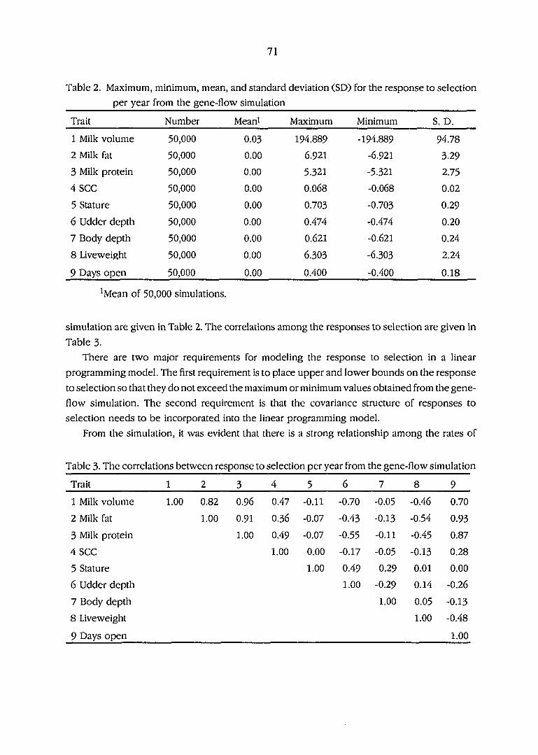
71
Table 2. Maximum, minimum, mean, and standard deviation (SD) for the response to selection
per year from the gene-flow simulation
Trait Number Meani Maximum Minimum S. D.
1 Milk volume 50,000 0.03 194.889 -194.889 94.78
2 Milk fat 50,000 0.00 6.921 -6.921 3.29
3 Milk protein 50,000 0.00 5.321 -5.321 2.75
4 see 50,000 0.00 0.068 -0.068 0.02
5 Stature 50,000 0.00 0.703 -0.703 0.29
6 Udder depth 50,000 0.00 0.474 -0.474 0.20
7 Body depth 50,000 0.00 0.621 -0.621 0.24
8 Liveweight 50,000 0.00 6.303 -6.303 2.24
9 Days open 50,000 0.00 0.400 -0.400 0.18
^Mean of 50,000 simulations.
simulation are given in Table 2. The correlations among the responses to selection are given in
Table 3.
There are two major requirements for modeling the response to selection in a linear
programming model. The first requirement is to place upper and lower bounds on the response
to selection so that they do not exceed the maximum or minimum values obtained from the gene-
flow simulation. The second requirement is that the covariance structure of responses to
selection needs to be incorporated into the linear programming model.
From the simulation, it was evident that there is a strong relationship among the rates of
Table 3. The correlations between response to selection per year from the gene-flow simulation
Trait 1 2 3 4 5 6 7 8 9
1 Milk volume 1.00 0.82 0.96 0.47 -0.11 -0.70 -0.05 -0.46 0.70
2 Milk fat 1.00 0.91 0.36 -0.07 -0.43 -0.13 -0.54 0.93
3 Milk protein 1.00 0.49 -0.07 -0.55 -0.11 -0.45 0.87
4 see 1.00 0.00 -0.17 -0.05 -0.13 0.28
5 Stature 1.00 0.49 0.29 0.01 0.00
6 Udder depth 1.00 -0.29 0.14 -0.26
7 Body depth 1.00 0.05 -0.13
8 Liveweight 1.00 -0.48
9 Days open 1.00

72
genetic gain for milk volume, fat, milk protein, somatic cell score, udder depth, liveweight, and
days open and also among the responses to selection for the three linear type traits. The objective
of developing constraints to mimic these relationships, is to restrict the feasible region of the
linear program to include only combinations of response to selection that are biologically
possible. Upper and lower bounds that enclose the feasible region among any two rates of
genetic gain were defined. Contours of the bivariate normal density function were used to
compute the upper and lower bounds for all correlations greater than 0.25 in absolute value.
Correlations of less than 0.25 in absolute value would have upper and lower bounds defining
the feasible region that were outside or close to the bounds defining the maximum or minimum
responses. The mathematical equations for this procedure are given in Appendix 1. Two
constraints were computed parallel to the major axis of the density ellipse and tangent to
ellipsoid at the intersection of the minor axis and the contour line. Eight further constraints were
computed tangent to the ellipse at the intersection of four lines parallel to the minor axis (see
Figure 1 A). The distances along the major axes from the intersection of the major and minor axes
for the four parallel lines were set to ±1/2 and ±1/3 of the length of the major axis. The constraints
were computed by using the upper 75% percentile of a chi-square distribution and were found
to provide a good approximation to the feasible region of the data from the simulation. At least
87% of the data from the simulation were contained within the bounding constraints for all pairs
of traits. Figure 1 illustrates the contours formed from the ten constraints used to model the
relationship between the rates of genetic gain for fat and protein production, (correlation 0.91).
Herd nutrition and liveweight constraints
The nutritional requirements for maintenance were modeled by using growth curves. The
liveweight at each start of lactation was computed from the von Bertanlanffy equation (Bakker
and Koops, 1978). To calculate liveweight profiles within lactation, cows were assumed to lose
0.46 kg of liveweight per day for the first 9 weeks of lactation (Satter and Roffler, 1975) and
assumed to gain weight linearly during the rest of the lactation and the subsequent dry period.
The gain in liveweight enabled cows to reach the projected liveweight at start of the next
lactation defined by the von Bertanlanffy equation. These liveweight profiles were used to
determine the average metabolic liveweight of the herd within parity for cows in different
physiological states—milking, dry, pregnant, and gaining and losing liveweight—these were
used in computing the nutritional requirements of the herd from NRC (1989) equations.
The response to selection in liveweight directly effects the metabolic liveweight. To account
for this, a constraint was included to compute the change in metabolic liveweight due to the
response to selection in liveweight.
A number of constraints were used to compute the herd metabolic liveweight for each year
of the planning horizon. The correlated response to selection for herd life was taken in account.
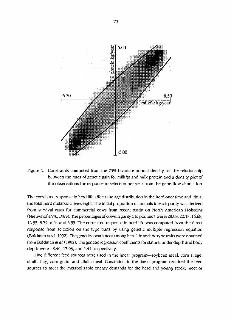
73
milkfat kg/year
Figure 1. Constraints computed from the 75% bivariate normal density for the relationship
between the rates of genetic gain for milkfat and milk protein and a density plot of
the observations for response to selection per year from the gene-flow simulation
The correlated response in herd life affects the age distribution in the herd over time and, thus,
the total herd metabolic liveweight. The initial proportion of animals in each parity was derived
from survival rates for commercial cows from recent study on North American Holsteins
(Nieuwhofe/a/., 1989). The percentages of cows in parity 1 to parities 7 were: 28.08,22.13,16.68,
12.33, 8.79, 6.04 and 5.95. The correlated response in herd life was computed from the direct
response from selection on the type traits by using genetic multiple regression equation
(Boldman etal., 1992). The genetic covariances among herd life and the type traits were obtained
from Boldman etal. (1992). The genetic regression coefficients for stature, udder depth and body
depth were -8.40, 17.03, and 1.44, respectively.
Five different feed sources were used in the linear program—soybean meal, corn silage,
alfalfa hay, corn grain, and alfalfa meal. Constraints in the linear program required the feed
sources to meet the metabolizable energy demands for the herd and young stock, meet or
74
exceed the demands for digestible protein, and provide a diet between 19% and 25% acid
detergent fiber. General recommendations from NRC (1989) suggest that this range of acid
detergent fiber in the diet of dairy cattle does not inhibit the feed intake of the cows nor adversely
effect milk production. Constraints also limited the amount of alfalfa hay and meal feed to 40%
on a kg dry-matter basis of the diet to avoid consumption of large amounts of these feeds, which
could inhibit intake owing to their bulkiness. The coefficients of the metabolizable energy
requirements for maintenance were calculated from NRC (1989) nutrition equations. The
coefficients of the metabolizable energy and digestible protein requirements (DPR) for milk
volume, fat, and milk protein production were taken from theoretical calculations reported by
Dado et al. (1990), assuming that 5% of the glucose requirements is provided by amino acids
and a 4.96% lactose concentration. The DPR requirement in kilograms for pregnancy, liveweight
gain and loss, and maintenance were computed by using ARC (1981) recommendations because
these emphasize the need to consider separately the nitrogen requirements of the microbial
population and the host animal in relation to energy intake.
The effects of correlated responses in herd life on the young stock feed requirements were
also taken into account when computing the total nutrient requirements of the herd, including
the herd replacements. A change in the age distribution of the herd in year t due to response
to selection for herd life will change the proportions of females replacements reared in years
t-1 and t-2, in as much as the replacements are reared over a 24-month period. Decreases or
increases in the proportions of replacements reared will reduce or increase the metabolizable
energy requirements for rearing replacements.
Milk production, mastitis, and somatic cell score constraints
The constraints for milk production (milk volume, fat, and protein) in year t accounted for
the response to selection for the milk production traits and the change in the milk production
traits due to genetic changes in herd life, SCS, and days open. The responses to selection for
milk, fat, and protein yields were transformed from mature equivalent (ME) production,
standardized for age, breed, region and month of calving to actual production by using USDA
adjustment factors (USDA 1974) for Holstein dairy cattle in the mid western region.
The effects of days open can affect herd milk production in two ways. First, days open may
effect the lactation yield. Thompson et al. (1982) have reported yield increases with increases
in days open. Funk etal. (1987) documented the affects of previous and present days open on
lactation yield. They derived correction factors for days open where a range of 9 consecutive
days open had the same correction factor. In this study, the maximum change in days open, due
solely to response to selection after 20 years of selection was approximately 9 days, and thus
should have little effect on lactation yield. The second effect of days open is to change the flow
of milk production over time. As days open increase, the time between the current and
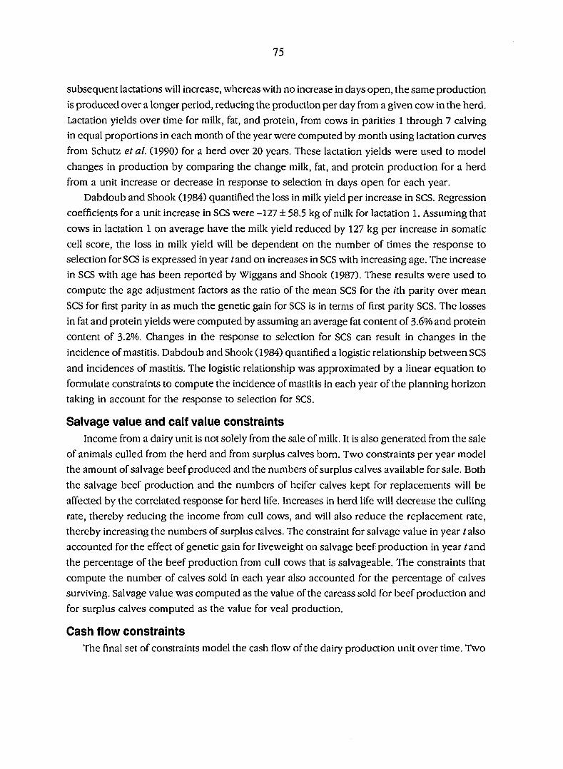
75
subsequent lactations will increase, whereas with no increase in days open, the same production
is produced over a longer period, reducing the production per day from a given cow in the herd.
Lactation yields over time for milk, fat, and protein, from cows in parities 1 through 7 calving
in equal proportions in each month of the year were computed by month using lactation curves
from Schutz etal. (1990) for a herd over 20 years. These lactation yields were used to model
changes in production by comparing the change milk, fat, and protein production for a herd
from a unit increase or decrease in response to selection in days open for each year.
Dabdoub and Shook (1984) quantified the loss in milk yield per increase in SCS. Regression
coefficients for a unit increase in SCS were -127 ± 58.5 kg of milk for lactation 1. Assuming that
cows in lactation 1 on average have the milk yield reduced by 127 kg per increase in somatic
cell score, the loss in milk yield will be dependent on the number of times the response to
selection for SCS is expressed in year fand on increases in SCS with increasing age. The increase
in SCS with age has been reported by Wiggans and Shook (1987). These results were used to
compute the age adjustment factors as the ratio of the mean SCS for the ith parity over mean
SCS for first parity in as much the genetic gain for SCS is in terms of first parity SCS. The losses
in fat and protein yields were computed by assuming an average fat content of 3.6% and protein
content of 3.2%. Changes in the response to selection for SCS can result in changes in the
incidence of mastitis. Dabdoub and Shook (1984) quantified a logistic relationship between SCS
and incidences of mastitis. The logistic relationship was approximated by a linear equation to
formulate constraints to compute the incidence of mastitis in each year of the planning horizon
taking in account for the response to selection for SCS.
Salvage value and calf value constraints
Income from a dairy unit is not solely from the sale of milk. It is also generated from the sale
of animals culled from the herd and from surplus calves born. Two constraints per year model
the amount of salvage beef produced and the numbers of surplus calves available for sale. Both
the salvage beef production and the numbers of heifer calves kept for replacements will be
affected by the correlated response for herd life. Increases in herd life will decrease the culling
rate, thereby reducing the income from cull cows, and will also reduce the replacement rate,
thereby increasing the numbers of surplus calves. The constraint for salvage value in year / also
accounted for the effect of genetic gain for live weight on salvage beef production in year /and
the percentage of the beef production from cull cows that is salvageable. The constraints that
compute the number of calves sold in each year also accounted for the percentage of calves
surviving. Salvage value was computed as the value of the carcass sold for beef production and
for surplus calves computed as the value for veal production.
Cash flow constraints
The final set of constraints model the cash flow of the dairy production unit over time. Two

76
cost constraints must be considered: fixed costs and variable cost per cow. Fixed costs are
defined as costs that are fixed regardless of the herd size and productive ability of the enterprise,
such as debt servicing, farm insurance, and farm maintenance. Variable costs refer to the costs
per cow such as breeding costs, housing costs, and labor, not costs due to feeding, and treatment
of mastitis.
The cash flow constraints compute the surplus or deficit in cash returns in each year and
account for the accrual of the surplus or deficit over time and the time value of money. The use
of a discount rate is the most common method for accounting for the time value of money
(Anderson et ah, 1977). In most animal breeding applications (McMahon etal., 1985), a nominal
interest rate is preferred. The purpose of using a discount rate is to account for the nominal
increase in the value of money, earned in the present year, in year t. This result can be achieved
by compounding the value each year by the appropriate interest rate. The approach used in this
model was to inflate cost and prices over time and account for the interest earned on a surplus
from year t-1 to year t or the cost of interest payments for a deficit from year t-1 to year t. The
procedure has the benefit of allowing the use of different inflation rates for costs and prices and
the use of different interest rates for surpluses and deficits.
Objective function
The objective function for the linear program was to maximize the accrued net income of
the dairy production enterprise at the end of the planning horizon. Because the cash flows for
each year are modeled as constraints in the linear program the objective function constisted of
maximizing the accrued cash flow surplus or minimizing the accrued cash flow deficit at the end
of the planning horizon.
Derivation of the economic value of response to selection
The linear programming model can be used to determine the amount of accrued net income
contributed from the cumulative response to selection due to sire selection. The economic
values could be used to rank sires in a selection index in terms of contributions to accrued net
producer income.
The economic values for the a trait can be derived as the change in accrued net income per
unit change in response to selection accounting for the effects of the response to selection for
the other eight traits simultaneously. These economic values can be obtained from the linear
programming model by using an extra constraint. If Gain/"^' and Gain/"'" denote the
allowable absolute value of the maximum and minimum response to selection per year for the
fth trait, then the extra constraint is
Gaiiii = Gain^"^ - UGainf"^'' + Gainf"" ) [31
where Xisa constant, which can take values from 0.00 to 1.00. The values used for X were 0.00

77
to 1.00 in 0.25 steps. The constraint in Eq. [3] is used to form separate linear programs for each
value of X and each of the nine traits, resulting in 45 linear programs. The results from each of
the 45 linear programs give the change in accrued net income from a restriction on one of the
responses to selection per year and the optimal values of the other eight responses to selection
given the restriction. These results can be used to derive the economic values by using the linear
model;
y = // + b'X + e [4]
where y is the vector of accrued net incomes, p, is the accrued net income when there is zero
response to selection in all traits, X is matrix of cumulative responses to selection, b is the vector
of unknown economic values, and e is the vector of residuals. The cumulative responses to
selection are computed as the rates of response to selection multiplied by the planning horizon.
The values for b can be solved from the normal equations using least squares (Snedecor and
Cochran, 1989).
Results and discussion
The linear programming model was used to compute optimal rates of response to selection
for four planning horizons; 1970-1989 (20 year), 1975-1989 (15 year), 1980-1989 (10 year), and
1985-1989 (5 year). A herd size of 80 milking cows was assumed. The price, cost, and interest
parameters used were representative for dairy production in the State of Iowa, USA. These
parameters are summarized in Table 4. The optimal response to selection per year for the four
planning horizons are given in Table 5. Tlie optimal response for herd life was computed directly
from the optimal responses for the three linear type traits. For all planning horizons, the optimal
responses to selection per year for individual traits were less than the maximum response to
selection per year achievable from the gene-flow simulation. The optimal responses per year
of genetic gain for the production traits was closest to the maximum acheivable rate. The rate
for fat was closest to its possible maximum value achieving 0.96 of the maximum rate for the
20, 15, and 10 planning horizons. Whereas the optimal response to selection per year for milk
and protein were closest to their possible maximum values achieving 0.94 and 0.92 of the
maximum rates, respectively, for the 5-year planning horizon. Of all the non-production traits,
days open had the greatest proportion of its maximum (0.73) due to its high correlations with
the production traits. The optimal responses per year were identical for the 20-, 15- and 10-year
planning horizons. This was due to payment for milk volume and fat content dominating the
net income for the first 17 years out of the 20 years studied. For each of the traits the optimal
responses per year for fat and liveweight (absolute value) were lower, whereas the optimal rate
for protein was greater for the 5-year planning honzon compared with the 20-, 15-, and 10-year
planning horizons. This due to drop in milk and fat payments and the increase in protein

Table 4. Price, cost, and interest rate parameters representative of Iowa, USA from 1970 to 1989^
Year 1970 1971 1972 1973 1974 1975 1976 1977 1978 1979 1980 1981 1982 1983 1984 1985 1986 1987 1988 1989
Prices Redeved
Milk $/I00kg 5.60 5.84 5.62 6.52 9.12 7.41 9.12 7.96 9.04 11.90 11.46 12.85 12.12 11.11 10.47 9.39 8.42 7.82 6.70 9.63
Fat S/kg 1.65 1.76 1.76 1.81 1.65 1.98 2.34 2.49 2.78 3.09 3.53 3.75 3.75 3.72 3.77 3.57 3.66 3.55 3.37 3.26
Protein $/kg 0.00 0.00 0.00 0.29 0.73 0.88 0.88 0.88 0.88 0.88 0.90 1.10 1.10 1.54 1.54 1.54 1.54 1.87 2.20 2.42
Calf veal $/kg 0.73 0.76 0.95 1.19 0.81 0.65 0.80 0.83 1.25 1.86 1.72 1.40 1.33 1.34 1.31 1.37 1.36 1.66 1.95 2.00
Beef S/kg 0.62 0.67 0.75 0.94 0.84 0.81 0.78 0.82 1.12 1.45 1.44 1.28 1.26 1.26 1.25 1.20 1.18 1.36 1.48 1.56
Costs of Production
Mastitis treatment S 30 35 39 47 59 63 74 76 85 98 104 115 117 122 125 125 127 131 134 145
Feed costs 2.12 2.18 1.95 2.96 4U3 4.07 4.04 3.95 3.81 4.15 4.17 5.15 4.22 4.70 5.07 4.33 4.07 4.07 4.28 5.41
S/lOOMcal
Variable costs $/cow 167 199 215 238 270 298 348 365 412 485 545 609 622 608 638 598 606 646 668 750
Fixed Costs $ 4921 4863 5257 5382 6479 7719 6914 7662 8416 9711 11232 13589 14882 15196 13561 12692 12091 11008 11631 11942
Interest Rates
Loan Payment % 7-91 5.72 5.25 8.02 10.8 7.86 6.84 6.82 9.06 12.67 15.26 18.87 14.86 10.79 12.04 9.93 8.33 8.22 9.32 10.87
Received % 5.95 4.88 4.50 6.44 7.83 6.25 5.50 5.46 7.46 10.28 11.77 13.41 11.02 8.50 8.80 7.69 6.33 5.66 6.20 6.93
^Source Iowa Agricultural Statistics (1972 through 1990) and Dunklee (1991)

79
Table 5 Optimal rates of genetic gain for four planning horizons
Planning Horizon
1970-1989 1975-1989 1980-1989 1985-1989
Milk kgy^ 183.52 183.52 183.52 183.30
Milkfat kgy^ 6.61 6.61 6.61 6.22
Protein kgy^ 4.49 4^9 449 4.88
Stature^ LTSy^ -0.57 -0.57 -0.57 -0.57
Udder Depth LTSy^ -0.16 -0.16 -0.16 -0.16
Body Depth LTSy^ -0.13 -0.13 -0.13 -0.13
Herd life daysy^ 1.92 1.92 1.92 1.92
SCS2 SCSy^ 4.8E-03 4.8E-03 4.8E-03 4.7E-03
Days Open days y 0.29 0.29 0.29 0.27
Liveweight kgy^ -3.58 -3.58 -3.58 -1.39
Accrued Net Income $U.S. 629104 685619 583606 275197
^LTS = Linear type score unit
-SCS = Somatic cell score
payments in the final 3 years of the 5 year planning horizon.
The relative economic value (REV) of a unit response to selection for each trait was
computed for each of the planning horizons. The value of the response is expressed as the value
of a unit genetic standard deviation gain relative to that for milk (value = 1.00) within each
planning horizon. Expression on a genetic standard deviation unit allows comparison of the
relative values free from the individual trait measurement units; e.g. kilograms versus days. The
REV for herd life was computed by including the cumulative response to selection for herd life
instead of the individual type traits in Eq. [4] . The REVs are given in Table 6. The REVs for
production traits are considerably larger than the REVs for the non-production traits for all
planning horizons. SCS had the largest REVs of the non-production traits in all planning horizons.
The REV of SCS was stable with the different lengths of planning horizon. This could be
attributable to the direct relationship between value of discarded milk from mastitis treatment,
milk prices, and the steady increase in mastitis treatment costs over time.
The cost and revenues in the first years of the planning horizon have the greatest impact on
accrued net income and also on the optimal rates of genetic gain and the REVs. For the
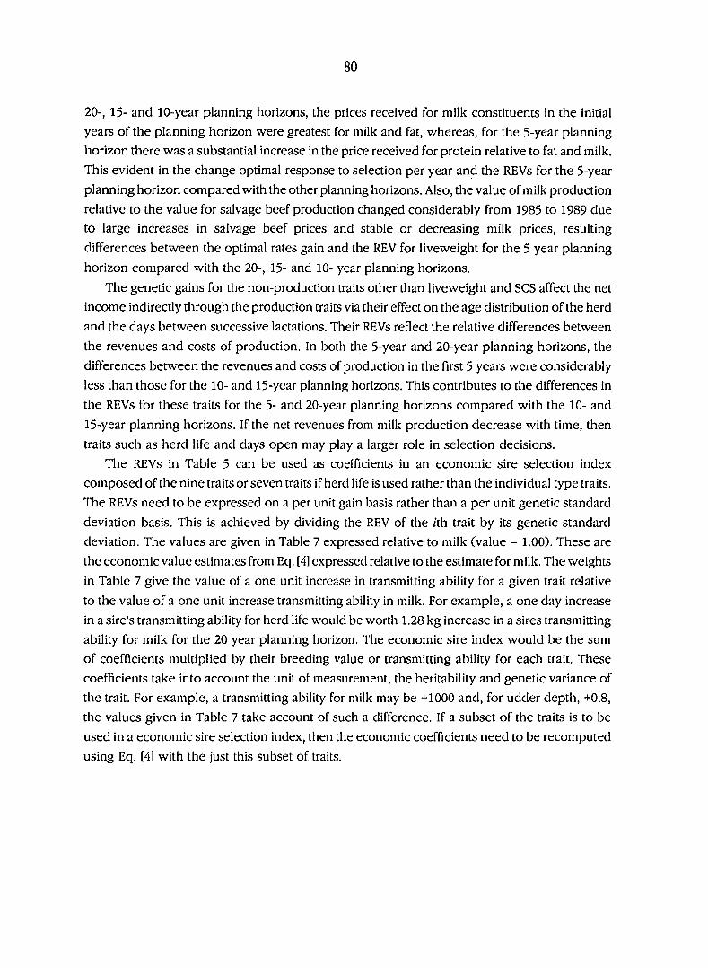
80
20-, 15- and 10-year planning horizons, the prices received for milk constituents in the initial
years of the planning horizon were greatest for milk and fat, whereas, for the 5-year planning
horizon there was a substantial increase in the price received for protein relative to fat and milk.
This evident in the change optimal response to selection per year and the REVs for the 5-year
planning horizon compared with the other planning horizons. Also, the value of milk production
relative to the value for salvage beef production changed considerably from 1985 to 1989 due
to large increases in salvage beef prices and stable or decreasing milk prices, resulting
differences between the optimal rates gain and the REV for liveweight for the 5 year planning
horizon compared with the 20-, 15- and 10- year planning horizons.
The genetic gains for the non-production traits other than liveweight and SCS affect the net
income indirectly through the production traits via their effect on the age distribution of the herd
and the days between successive lactations. Their REVs reflect the relative differences between
the revenues and costs of production. In both the 5-year and 20-year planning horizons, the
differences between the revenues and costs of production in the first 5 years were considerably
less than those for the 10- and 15-year planning horizons. This contributes to the differences in
the REVs for these traits for the 5- and 20-year planning horizons compared with the 10- and
15-year planning horizons. If the net revenues from milk production decrease with time, then
traits such as herd life and days open may play a larger role in selection decisions.
The REVs in Table 5 can be used as coefficients in an economic sire selection index
composed of the nine traits or seven traits if herd life is used rather than the individual type traits.
The REVs need to be expressed on a per unit gain basis rather than a per unit genetic standard
deviation basis. This is achieved by dividing the REV of the /th trait by its genetic standard
deviation. The values are given in Table 7 expressed relative to milk (value = 1.00). These are
the economic value estimates from Eq. [4] expressed relative to the estimate for milk. The weights
in Table 7 give the value of a one unit increase in transmitting ability for a given trait relative
to the value of a one unit increase transmitting ability in milk. For example, a one day increase
in a sire's transmitting ability for herd life would be worth 1.28 kg increase in a sires transmitting
ability for milk for the 20 year planning horizon. The economic sire index would be the sum
of coefficients multiplied by their breeding value or transmitting ability for each trait. These
coefficients take into account the unit of measurement, the heritability and genetic variance of
the trait. For example, a transmitting ability for milk may be +1000 and, for udder depth, +0.8,
the values given in Table 7 take account of such a difference. If a subset of the traits is to be
used in a economic sire selection index, then the economic coefficients need to be recomputed
using Eq. [4] with the just this subset of traits.
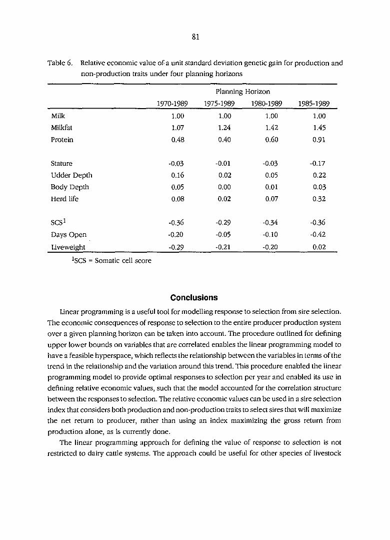
81
Table 6. Relative economic value of a unit standard deviation genetic gain for production and
non-production traits under four planning horizons
1970-1989
Planning Horizon
1975-1989 1980-1989 1985-1989
Milk 1.00 1.00 1.00 1.00
Milkfat 1.07 1.24 1.42 1.45
Protein 0.48 0.40 0.60 0.91
Stature -0.03 -0.01 -0.03 -0.17
Udder Depth 0.16 0.02 0.05 0.22
Body Depth 0.05 0.00 0.01 0.03
Herd life 0.08 0.02 0.07 0.32
scsi -0.36 -0.29 -0.34 -0.36
Days Open -0.20 -0.05 -0.10 -0.42
Liveweight -0.29 -0.21 -0.20 0.02
^SCS = Somatic cell score
Conclusions
Linear programming is a useful tool for modelling response to selection from sire selection.
The economic consequences of response to selection to the entire producer production system
over a given planning horizon can be taken into account. The procedure outlined for defining
upper lower bounds on variables that are correlated enables the linear programming model to
have a feasible hyperspace, which reflects the relationship between the variables in terms of the
trend in the relationship and the variation around this trend. This procedure enabled the linear
programming model to provide optimal responses to selection per year and enabled its use in
defining relative economic values, such that the model accounted for the correlation structure
between the responses to selection. The relative economic values can be used in a sire selection
index that considers both production and non-production traits to select sires that will maximize
the net return to producer, rather than using an index maximizing the gross return from
production alone, as is currently done.
The linear programming approach for defining the value of response to selection is not
restricted to dairy cattle systems. The approach could be useful for other species of livestock
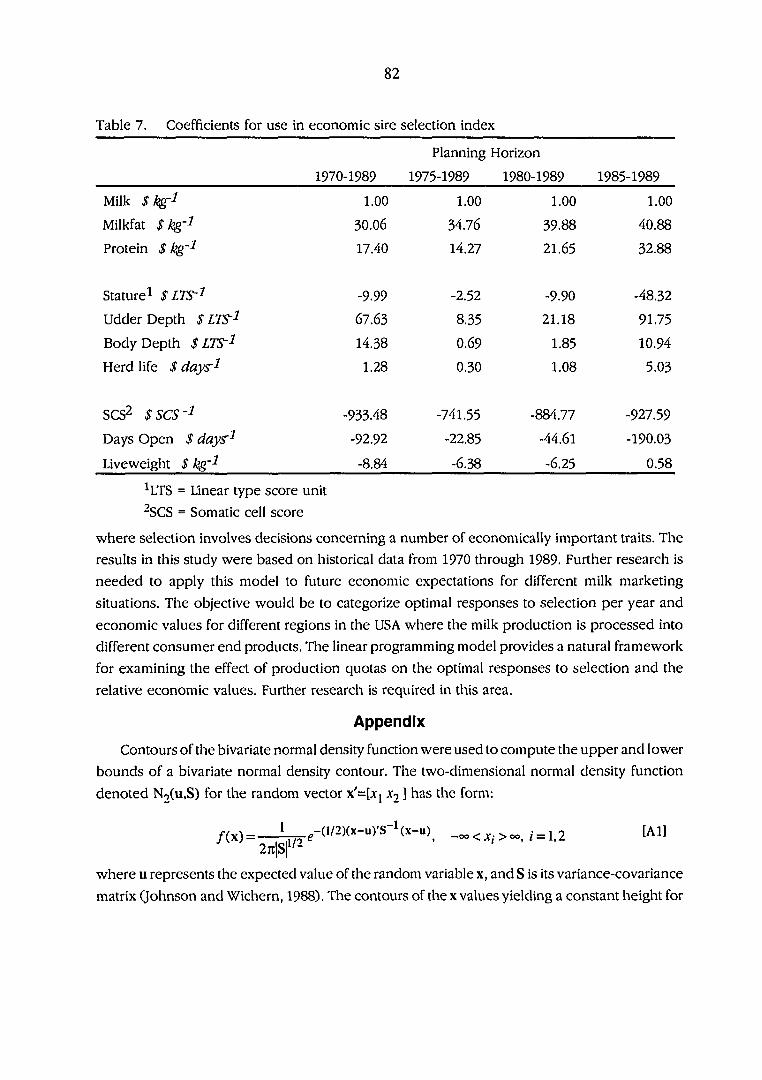
82
Table 7. Coefficients for use in economic sire selection index
Planning Horizon
1970-1989 1975-1989 1980-1989 1985-1989
Milk $ kg-^ 1.00 1.00 1.00 1.00
Milkfat $ kg'^ 30.06 34.76 39.88 40.88
Protein $ kg'^ 17.40 14.27 21.65 32.88
Stature! $ LTS-^ -9.99 -2.52 -9.90 -48.32
Udder Depth $ LTS-^ 67.63 8.35 21.18 91.75
Body Depth $ LTS'^ 14.38 0.69 1.85 10.94
Herd life $ clays'^ 1.28 0.30 1.08 5.03
SCS2 $SCS-^ -933.48 -741.55 -884.77 -927.59
Days Open $ ciays"^ -92.92 -22.85 -44.61 -190.03
Liveweight S kg'^ -8.84 -6.38 -6.25 0.58
^LTS = Linear type score unit
"SCS = Somatic cell score
where selection involves decisions concerning a number of economically important traits. The
results in this study were based on historical data from 1970 through 1989. Further research is
needed to apply this model to future economic expectations for different milk marketing
situations. The objective would be to categorize optimal responses to selection per year and
economic values for different regions in the USA where the milk production is processed into
different consumer end products. The linear programming model provides a natural framework
for examining the effect of production quotas on the optimal responses to selection and the
relative economic values. Further research is required in this area.
Appendix
Contours of the bivariate normal density function were used to compute the upper and lower
bounds of a bivariate normal density contour. The two-dimensional normal density function
denoted NjCu.S) for the random vector ^ ] has the form;
/(X) = 1 g-(l/2)(x-uyS-l(x-u)^ -oo<;C,.>oo, / = l,2 [Al] 27clSf'-
where u represents the expected value of the random variable x, and S is its variance-covariance
matrix (Johnson and Wichern, 1988). The contours of the x values yielding a constant height for
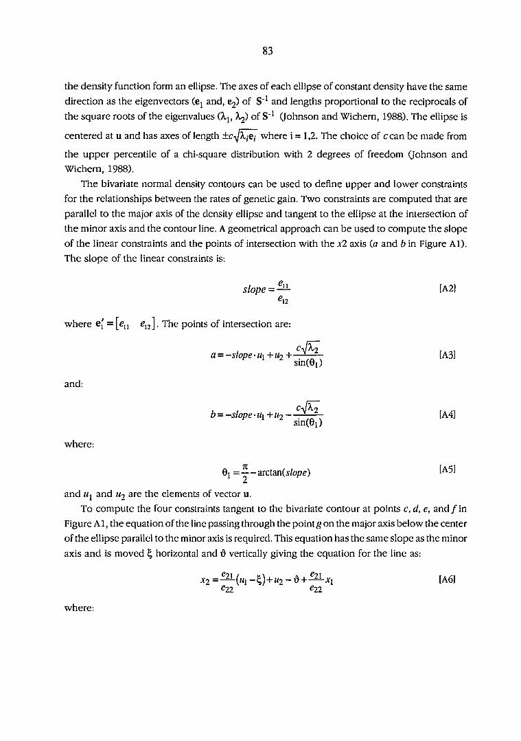
83
the density function form an ellipse. The axes of each ellipse of constant density have the same
direction as the eigenvectors (ej and, 62) of S'^ and lengths proportional to the reciprocals of
the square roots of the eigenvalues (A,|, of S"^ (Johnson and Wichern, 1988). The ellipse is
centered at u and has axes of length ±c-^A,/e/ where i = 1,2. The choice of ccan be made from
the upper percentile of a chi-square distribution with 2 degrees of freedom (Johnson and
Wichern, 1988).
The bivariate normal density contours can be used to define upper and lower constraints
for the relationships between the rates of genetic gain. Two constraints are computed that are
parallel to the major axis of the density ellipse and tangent to the ellipse at the intersection of
the minor axis and the contour line. A geometrical approach can be used to compute the slope
of the linear constraints and the points of intersection with the x2 axis (a and t> in Figure Al).
The slope of the linear constraints is:
slope - — [A2] 12
where e[ = [g,, g,;]. The points of intersection are:
sin(0i)
c u r a = -slope • Ml + «2 + . [A3]
and:
sin(0i)
where:
01 = Y-arctan(s/ope)
c \X~ b = -slope • Ml +1(2 —. "• [A4]
[A5]
and «1 and «2 ^re the elements of vector u.
To compute the four constraints tangent to the bivariate contour at points c, d, e, and/in
Figure Al, the equation of the line passing through the point g on the major axis below the center
of the ellipse parallel to the minor axis is required. This equation has the same slope as the minor
axis and is moved ^ horizontal and û vertically giving the equation for the line as:
A'2 ='^^(mi —^)+M2 —iS'H—— 1 [A6] ^22 " ^22
where:
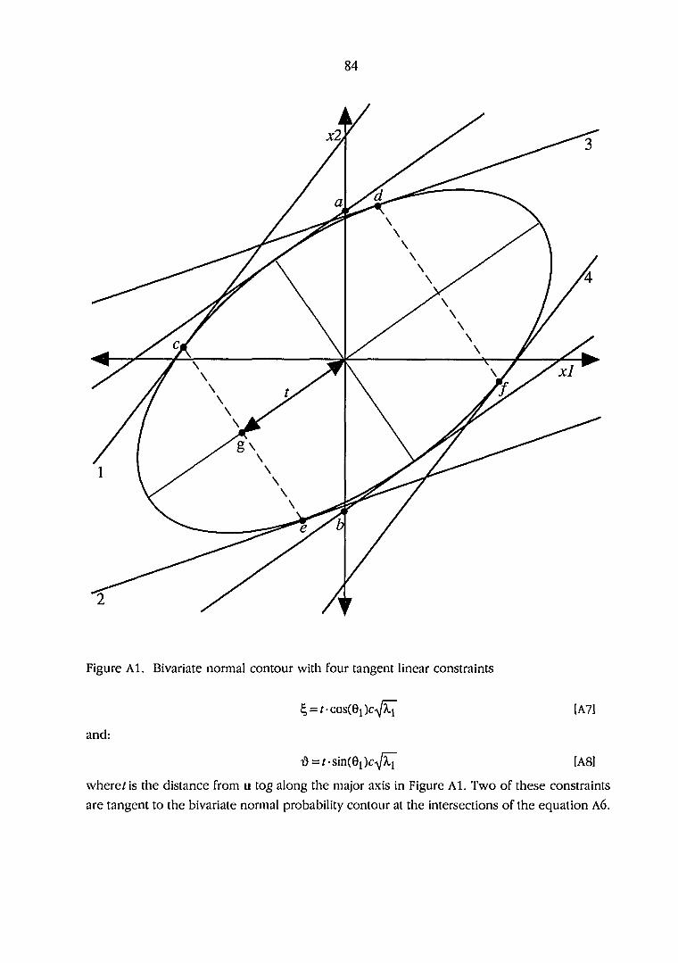
84
Figure Al. Bivariate normal contour with four tangent linear constraints
^ = t^cos{Ql)c^|ï^ [A7]
and:
û = t-sm(Qi)c^m [A8]
where^ is the distance from u tog along the major axis in Figure Al. Two of these constraints
are tangent to the bivariate normal probability contour at the intersections of the equation A6.

85
The points of intersection are obtained by solving the following two sets of equations
simultaneously:
f { \ ) = (x - u)'S~^(x - u) - ,
—^Xi + A'2 = — %) + «2 [A9] ^22 ^22
obtaining two solutions for the vector x, say, Yi and yj, corresponding to the two points of
intersection, c and e in Figure Al. The slope of a point on the contour can be found be examining
the first derivative of the bivariate normal probability contour. The slopes at c and e are:
3F(x)/3A-2
and:
[AlO] yi
[All] y i d f (x ) ldx2
The ellipsoid is symmetric therefore constraints 1 and 4 and constraints 2 and 3 in Figure Al have
the same slope. Because yj, y2, slope^ and slope2 have been defined, giving the equations for
constraints 1 and 2 in Figure Al, a geometric approach can be used to derive the equations for
constraints 3 and 4 from the symmetrical nature of the bivariate normal probability contour. The
equations for the four constraints are.
constraint 1:X2 = slopei -yn +yi2 +slopei-xi
constraint 2 : X2 = -slopei • >"21 + >"22 + slope2 • X\
constraint 3 : X2=-slopei(yii +2^)+yi2+2û+slopei -Xi
constraint 4 : = -5/0/7^2(>"21 +2^)+>>22 + 2û+slope2-xi
where is the yth element of y,- vector, and /= 1,2.

86
REFERENCES
Ali, A. K. A., and G. E. Shook. 1979- An optimum transformation for somatic cell concentration
in milk. /. Dairy. Set 63:487.
Ali, T. E., and L. R. Schaeffer. 1987. Sire-son correlations of genetic evaluations for fat percentage
in Holstein-Friesians. Can.J. Anim. Set 67:631.
Allaire, F. R., and C. S. Thaen. 1985. Perspectives for genetic improvement in economic efficiency
of dairy cattle. J. Dairy Sci. 68:3110.
Anderson, J. R., J. L. Dillion, and J. B. Hardaker. 1977. Agricultural decision analysis. Iowa State
University Press, Ames.
Anderson, R. D., R. W. Miller, and L. D. VanVleck. 1978. Economic analysis of protein testing for
selection. / Dairy Sci. 61:102.
Andrus, D. F., and L. D McGillard. 1975. Selection of dairy cattle for overall excellence./. Dairy
Sci. 58:1876
ARC 1981. The nutrient requirements of ruminant livestock. Commonwealth Agricultural
Bureaux. Gresham Press, Surrey UK.
Badinga, L, R.J. Collier, C.J. Wilcox, and W. W. Thatcher. 1985. Interrelationships of milk yield,
body weight and reproductive performance. /. Dairy. Sci. 68:1828.
Bakker, H., and W. J. Koops. 1978. An approach to the comparison of growth curves of Dutch
Friesian, British Friesian and Holstein Friesian cows. Patterns of growth and development
in cattle., Ed H. de Boor and J Martin, Martin Nijhoff Publ. The Hague, Tlie Netherlands.
Balaine, D. S., R. E. Pearson, and R. H. Miller. 1981. Repeatability of net economic efficiency in
dairy cattle and the role of some economic variables as its predictors. / Daily Sci. 64:96.
Bancs, G., and G. E. Shook. 1990. Genotype by environment interaction and genetic correlation
for somatic cell count and milk yield. / Dairy Sci. 73:2563.
Bartlett, P. C., G. Y. Miller, C. R. Anderson, andj. H. Kirk. 1990. Milk production and somatic cell
count in Michigan dairy herds. /. Dairy Sci. 73:2794.
Berger, P. J., R. D. Shanks, A. E. Freeman, and R. C. Laben. 1981. Genetic aspects of milk yield
and reproductive performance. J. Dairy. Sci. 64:114.
Blosser, T. H. 1979. Economic losses from and the national research program on mastitis in the
United States. /. Dairy Sci. 62:119.
Boldman, K. G., A. E. Freeman, B. L. Harris, and A. L. Kuck. 1992. Prediction of sire transmitting
abilties for linear type score. /. Dairy Sci. (in press)
Brascamp, E. W. 1973. Model calculations concerning economic optimization of A. I. breeding
cattle. Z. Tierz. Zuechtimgsbiol. 90:1.
Brascamp, E. W., and Minkema, D. 1972. Economic aspects of selection for milk, fat%, and
protein% in a dairy cow AI population. Z. Tierzttcbtg. Zûchtgsblol. 89:99.

87
Brascamp, E. W., C. Smith, and D. R. Guy. 1985. Derivation of Economic weights from profit
equations. Anim. Prod. 40:1975.
Bulmer, M. G. 1980. Tlje mathematical tbeoty of quantitative genetics. Clarendon Press, Oxford
U.K.
Clark, R. D., and R. W. Touchberry. 1962. The effect of body weight and age at calving on milk
production in Holstein cattle. J. Dairy Sci. 45:1500.
Coffey, E. M., W. E. Vinson, and R. E. Pearson. 1985. Heritabilities for lactation average somatic
cell counts in first, second, third and later parities. J. Dairy Sci. 68:3360.
Cochran, W. G. 1951. Improvement by means of selection. InProc. 2nd Berkeley Symp. Math. Stat.
Prob. (ed. J. Newman) pp. 449-70. University of California Press, Berkeley.
Cue, R. I., H. G. Monardes, andJ. F. Hayes. 1987. Correlations between production traits in first
lactation Holstein cows. J. Dairy Sci. 70:2132.
Cunningham, E. P. 1975. Multi-stage index selection. Vjeor. andAppl. Genet. 74:753.
Curnow, R. N. 1961. The estimation of repeatability and heritability from records subject to culling.
Biometrics 17:553.
Dabdoub, A., and G. E. Shook. 1984. Phenotypic relationships among milk yield, somatic cell
count, and clinical mastitis./. Dairy Sci. Suppl. 1. 67:234,
Dado, A. A., D. R. Mertens, and G. E. Shook. 1990. Theoretical metabolizable energy and protein
requirements for milk component production. J. Dairy Sci. Suppl. 73:248.
Dentine, M. R., and B. T. McDainel. 1987. Expected genetic gain for milk yield in diary cattle.
Theor. and Appt. Gen. 74: 753
de Jager, D., and B. W. Kennedy. 1987. Genetic parameters of milk yield and composition and
their relationships with alternative breeding goals. / Dairy Sci. 70:1258.
Dickerson, G. E., and L. N. Hazel. 1944. Effectiveness of selection on progeny performance as a
supplement to earlier culling in livestock. J. Agric. Res. 69, 459-76.
Donimerholt, J. and J. B. M. Wilmink. 1986. Optimal selection responses under varying milk prices
and margins for milk production. Livest. Prod. Sci. 14:109
Ducrocq, V., and R. L. Quaas. 1988. Prediction of genetic response to truncation selection across
generations. J. Dairy Sci. 71: 2543.
Elsen,J. M., and J. C. Mocquot. 1974. Recherches pour une rationalisation technique des schémas
desélection des bovins et ovins. Bulletin Tech. Dep. Génét. Animal Inst. Natl. Rech. Agron.
17, Jouy-en-Josas. France.
Emanuelson, U., B. Danell, and J. Philipsson. 1988. Genetic parameters for clinical mastitis,
somatic cell counts, and milk production estimated by multiple-trait restricted maximum
likelihood./. Dairy Sci. 71:467.
Falconer, D. S. 1989. Introduction to quantitative genetics. Longman Scientific and Technical,

88
Longman Group UK LTD., Essex, U.K.
Fisher, R.A. 1936. The use of multiple measurements in taxonomic problems. Annals Eugenics
(London) 7:240.
Fisher, R. A., and F. Yates. 1953. Statistical tables for biological, agricultural and medical research.
4th edn. Oliver and Boyd, London, U.K.
Foster, W. W., A. E. Freeman, P.J. Berger, and A. Kuck. 1988. Linear type trait analysis with genetic
parameter estimation./. Dairy Sci. 71:223.
Freeman, A. E. 1976. Management traits in dairy cattle, dystocia, udder characteristics related to
production, and a review of other traits. Livest. Prod. Sci. 3:13.
Freeman, A. E. 1984. Secondary traits: Sire evaluation and the reproductive complex./. Dairy Sci.
67:449.
Freeman, A. E. 1986. Genetic control of reproduction and lactation in dairy cattle. Proc. of the
World Congress to Applied Livestock Production, Ed. G. E. Dickerson and R. K. Johnson,
University of Nebraska, Lincoln NE, 11:3.
Funk, D. A., A. E. Freeman, and P.J. Berger. 1987. Effects of previous days open, previous days
dry and present days open on lactation yield. /. Dairy Sci. 70:2366.
Gibson, C. D. 1976. An economic model for deriving economic values for the use in selection
indexes. M. Sc. Thesis, Iowa State Univ., Ames.
Gibson, J. P. 1987. The options and prospects for genetically altering milk composition in dairy
cattle. Anim. Breed. Abstr. 55:231.
Gibson, J. P. 1989a. Selection on the major components of milk: alternative methods for deriving
economic weights. /. Dairy Sci. 72:3176.
Gibson, J. P. 1989b. The effects of pricing systems, economic weights, and population parameters
on economic response to selection on milk components. /. Daity Sci. 72:3314.
Gill, G. S., and F. R. Allaire. 1976a. Relationship of age at first calving, days open, days dry, and
herd life to a profit function for dairy cattle. /. Daity Sci. 64:1131.
Gill, G. S., and F. R. Allaire. 1976b. Genetic and phenotypic parameters for profit function and
selection method for optimizing profit in dairy cattle. /. Daity Sci. 64:1325.
Gonyon, D. S., D. O. Everson, and R. E. Christian. 1982. Heritability of mastitis score in Pacific
Northwest dairy herds. /. Daity Sci. 65:1269.
Greon, A. F. 1988. Derivation of economic values in cattle breeding: A model at the farm level.
Agricultural Systettis 27:195.
Greon, A. F. 1989a. Economic values in cattle breeding. I. Influences of production circumstances
in situations without output limitations. Livest. Prod. Sci. 22:1.
Greon, A. F. 1989b. Economic values in cattle breeding. II. Influences of production circumstances
in situations with output limitations. Livest. Prod. Sci. 22:17.
Hanna, M. V., and E. P. Cunningham. 1974. Selection alternatives for improving the yield of milk
89
and its constituents in Irish dairy cattle. Irish J. Agrlc. Res. 13:239.
Hansen, L. B., A. E. Freeman, and P. J. Berger. 1983a. Variances, repeatabilities, and age
adjustments of yield and fertility in dairy cattle./. Dairy Set. 66:281.
Hansen, L. B., A. E. Freeman, and P.J. Berger. 1983b. Yield and fertility relationships in dairy cattle.
J. Dairy Sci. 66:293.
Hargrove, G. L., D. A. Mbah, and J. L. Rosenberger. 1981. Genetic and environmental influences
on milk and milk component production./. Dairy Sci. 64:1593.
Harris, B. L., and A. E. Freeman. 1991. Prediction of response with overlapping generations
accounting for multistage selection. Theor. and Appl. Genet. 82:329.
Harris, D. L. 1970. Breeding for efficiency in livestock production: Defining the economic
objectives. Anini. Sci. 30:860
Harville, D. A. and C. R. Henderson. 1966. Interrelationships among age, body weight and
production traits during first lactation of dairy cattle. /. Dairy Sci. 49:1249.
Hazel, L. N. 1943. The genetic basis for constructing selection indexes. Genetics 28:476.
Hazel, L. N. 1956. Selection Indexes. Mimeographed. Department of Animal Science, Iowa State
University, Ames.
Henderson, C. R. 1952. Specific and general combining ability. Heterosis. Iowa State University
Press, Ames.
Henderson, C. R. 1963. Selection indexes and expected genetic advance. Statistical Genetics and
Plant Breeding, NAS-NRC 9S2:\
Hill, W. G. 1974. Prediction and evaluation of response to selection with overlapping generations.
Anitn. Prod. 18:124.
Hill, W. G. 1979. A note on effective population size with overlapping generations. Genetics
92:317.
Hillers, J. K. 1984. Sire selection under alternative systems of milk pricing. /. Dairy Sci. 67:444.
Hoque, M., and J. Hogdes. 1980. Genetic and phenotypic parameters of lifetime production traits
in Holstein cows./. Dairy Sci. 63:1900.
James, J. W. 1978. Effective population size in open nucleus breeding schemes. Acta Agriculturœ
Scandinavica 28:388.
James, J. W. 1982. Economic aspects of developing breeding objectives: General considerations.
Future developments in the genetic improvement of Animals. Academic Press, Sydney,
Australia
Johnson, D. L. 1977. Inbreeding in populations with overlapping generations. Genetics SI:5Sl.
Johnson, R. A., and , D. W. Wichern. 1988. Applied multivariate statistical analysis. 2nd Edition.
Prentice Hall, Englewood Cliffs, New Jersey, USA.
Jansen, G. B., and, J. W. Wilton. 1984. Linear programming in livestock. /. Dairy Sci. 67:897.

90
Jansen, J. 1985. Genetic aspects of fertility in dairy cattle based on analysis of A. I. data-A review
with emphasis on areas for further research. Livest. Prod. Set. 12:1.
Jansen, J., J. Van Der Werf, and W. Boer. 1987. Genetic relationships between fertility traits for
dairy cows in different parities. Livest. Prod. Sci. 17:337.
Keller, D. S., and F. R. Allaire. 1990. Economic weights for genetic changes in milk component
yields at the herd level. / Dairy Sci. 73:1631.
Kennedy, B. W., M. S. Sethar, J. E Moxely, and B. R. Downey. 1982. Heritability of somatic cell
count and its relationship to milk yield and composition in Holsteins./. Dairy Sci. 65:843.
Kragelund, K., J. Hillel, and K. Kalay. 1979. Genetic and phenotypic relationships between
reproduction and milk production. 5c/. 62:468.
Ladd, G. W. 1982. A product-characteristic approach to technical change: with application to
animal breeding. In Economic analysis and agricultural policy. Ed. R. Day. Iowa State
University Press, Ames.
Lawstuen, D. A., L. B. Hansen, G. R. Steuernagel, and L. P. Johnson. 1988. Management traits
scored linearly by dairy producers./. Dairy Sci. 71:788.
Legates, J. E. and C. D. Grinnells. 1952. Genetic relationships in resistance to mastitis in dairy cattle.
/. Dairy Sci. 35:289.
Lin, C. Y. 1978. Selection index for genetic improvement of quantitative characters. Tfjeor. and
Appl. Genet., 52:49.
Lin C. Y., and F. R. Allaire. 1977. Relative efficiency of selection methods for profit in dairy cattle.
/ Daily Sci. 60:1970.
Lin C. Y., and F. R. Allaire. 1978. Efficiency of selection on milk yield to a fixed age. / Dairy Sci.
61:489.
Lin, C. Y., A.J. McAllister, and A.J. Lee. 1985. Multitrait estimation of relationships of first lactation
yields to body weight changes in Holstein heifers. / Dairy Sci. 63:1900.
Maijala, K. 1964. Fertility as a breeding problem in artificially bred populations of dairy cattle. I.
Registration and heritability. Ann. Agric. Fenn., 3- Siippl. 1:94.
Maijala, K. 1976. Possibilities for improved reproduction in cattle by selection. World Rev. Anim.
Prod. 12:69.
Maijala, K., and M. Hanna. 1974. Reliable phenotypic and genetic parameters in dairy cattle. Proc.
1st World Congress on Genet. Appl. Livest. Prod., Madrid. Vol. 1:541.
Manfredi, E. J., R. W. Everett, and S. R. Searle. 1984. Phenotypic and genetic statistics of
components of milk and two measures of somatic cell concentration./ Dairy Sci. 67:2028.
McClintock, A. E., and E. P. Cunningham. 1974. Selection in dual purpose cattle populations: effect
of beef crossing and cow replacement rates. Annals Genêt. Sél. Animal 6:227.
McMahon, R. T., R. W. Blake, C. R. Shumway, D.J. Leathem, M. A. Tomaszewski, and K. R. Butcher.
1985. Effects of planning horizon and conception rates on profit maximizing selection of
91
artificial insemination sires. J. Dairy Sci. 68:2295.
Melton, B. E., O. Heady and R. L. Willham. Estimation of economic values for selection indices.
Anim. Prod. 28:279
Meyer, K. 1984. Estimates of genetic parameters for milk and fat yield for the first three lactations
in British Friesian Cows. Anim. Prod. 38:313.
Meyer, K. 1985. Genetic parameters of dairy production of Australian black and white cows. Livest.
Prod. Sci. 12:205.
Meyer, K., Brotherstone, S., W. G. Hill, and M. R. Edwards. 1987. Inheritance of linear type traits
in dairy cattle and correlations with milk production. Anim. Prod. 44:1.
Miller, R. H. 1984. Traits for sire selection related to udder health and management. / Dairy Sci.
67:459.
Miller, R. H., and L. D. McGillard. 1959. Relations between weight at first calving and milk
production during first lactation./. Dairy Sci. 42:1932.
Miller, R. H., and R. E. Pearson. 1979. Economic aspects of selection. Anim. Breeding Abstr. 47:281.
Miller, R. H., M. Lukaszewick, and R. E. Pearson. 1981. Dual-purpose selection in dairy cattle. Z.
Tierzilchtg. Zûcbtgsbiol. 98:108.
Moav, R. 1966a. Specialised sire and dam lines. I. Economic evaluation of crossbreds. Anim. Prod.
8:193.
Moav, R. 1966b. Specialised sire and dam lines. II. The choice of the most profitable parental
combination when component traits are genetical additive. Anim. Prod. 8:203.
Moav, R. 1966c. Specialised sire and dam lines. III. The choice of the most profitable parental
combination when component traits are genetical non-additive. Anim. Prod. 8:365.
Moav, R. 1973. Economic evaluation of genetic differences. In Agricultural genetics: selected
topics. Ed. by R. Moav. John Wiley and Sons, New York, USA.
Moav, R., and W. G. Hill 1966. Specialised sire and dam lines. IV. Selection within lines. Anim.
Prod. 8:375.
Monardes, H. G., B. W. Kennedy, and J. E. Moxely. 1983. Heritabilities of measures of somatic
cell count per lactation. J. Dairy Sci. 66:1707.
Monardes, H. G., and J. F. Hayes. 1985. Genetic and phenotypic statistics of lactation cell counts
in different lactations of Holstein cows./. Dairy Sci. 68:1449.
Moore R. K., B. W. Kennedy, L. R. Schaeffer, and J. E. Moxely. 1990. Relationships between
reproduction traits, age and body weight at calving in first lactation Ayrshires and Holsteins.
/. Daily Sci. 73:835.
Moore R. K., B. W. Kennedy, L. R. Schaeffer, and J. E. Moxely. 1991. Relationships between age
and body weight and production in first lactation Ayrshires and Holsteins. /. Dairy Sci.
74:269.

92
Nieuwhof G. F., H. D. Norman, and F. N. Dickerson. 1989. Phenotypic trends in herd life of dairy
cows in United States./. Dairy Sci. 72:726.
Norman, H. D., and F. N. Dickerson. 1971. An economic index for determining the relative value
of milk and fat in predicted differences of bulls and cow index values for cows. Dairy Herd
Improvement Lett. 47:1.
NRG 1989. Nutrient requirements of dairy cattle. Sixth revised Edition Update 1989. National
Academy Press, Washington, D. C., USA
Pearson, R. E., and R. E. Miller. 1979. Economic definition of total performance, breeding goals
and breeding values for dairy cattle. J. Dairy Sci. 64:857.
Philipsson, J. 1981. Genetic aspects of female fertility in dairy cattle. Livest. Prod. Sci. 8:307.
Raubertas, R. F., and G. E. Shook. 1982. Relationship between lactation measures of somatic cell
concentration and milk yield. / Dairy Sci. 65:419.
Rendel, J. M., and A. Robertson 1950. Estimation of genetic gain in milk yield by selection in a
close herd of dairy cattle. J. Genetics 50:1.
Schaeffer, G. B., W. E. Vinson, R. E. Pearson, and R. G. Long. 1985. Genetic and phenotypic
relationships among type traits scored linearly in Holsteins. J. Dairy Sci. 68:2984.
Schutz, M. M., L. B. Hansen, G. R. Steuemagel, J. K. Reneau, and A. L. Kuck. 1990. Genetic
parameters for somatic cells, protein, and fat in milk for Holsteins. J. Dairy Sci. 73:494.
Sechrist, R. S. 1985. Summary of NCDHIPpolicies. Natl. Coop. Dairy Herd Improvement Prog.
Handbook, Fact Sheet B-3.
Seykora, A. J., and B. T. McDaniel. 1983. Heritabilities and correlations of lactation yields and
fertility for Holsteins. J. Dairy Sci. 66:1486.
Shook, G. E. 1982. Prvspectsfor genetic improvement in mastitis resistance. Meeting of NC-2 and
S-49 Regional Research projects on dairy cattle breeding. Indianapolis, IN.
Smith, C., J. W. James, and E. W. Brascamp. 1986. On the derivation of economic weights in
livestock improvement. Anirn. Prod. 43:545.
Smith, H. F. 1936. A discriminant function for plant selection. Annuals of Eugenics (London)! :ll^.
Snedecor, G. W., and W. G. Cochran. 1989. Statistical Methods. Eighth edition. Iowa State
University Press, Ames.
Sposito, V. A. 1989. Linearprograrnrning with statistical applications. Iowa State University Press,
Ames.
Swalve, H., and L. D. VanVleck. 1987. Estimation of genetic (co)variances for milk yield in the
first three lactations using an animal model and restricted maximum likelihood./ Dairy Sci.
70:842.
Teepker, G., and H. H. Swalve. 1988. Estimation of genetic parameters for milk production in the
first three lactations. Livest. Prod. Sci. 20:193.
Thompson, J. R., A. E. Freeman, and P.J. Berger. 1980. Variation of traits of a mating appraisal

93
program. / Daiiy Sci. 63:133.
Thompson, J. R., A. E. Freeman, D.J. Wilson, C. A. Chapin, P.J. Berger, and L. P.Johnson. 1981.
Evaluation of a linear type program in Holsteins./. Dairy Sci. 64:l6lO.
Thompson,J. R., A. E. Freeman, and P.J. Berger. 1982. Days open adjusted, annualized, and fat
corrected yield as alternatives to mature equivalent records. / Dairy Sci. 65:1562.
Thompson, J. R., K. L. Lee, A. E. Freeman, and L. P.Johnson. 1983. Evaluation of a linearized type
appraisal system for Holstein cattle. / Dairy Sci. 66:325.
Tong, A. K. W., B. W. Kennedy, and J. E. Moxely. Heritabilities and genetic correlations for the
first three lactations form records subject to culling. / Dairy Sci. 62:1784.
Van Arendonk, J. A. M., R. Hovenier, and W. De Boer. 1989. Phenotypic and genetic association
between fertility and production in dairy cows. Livest. Prod. Sci. 21:1.
Vinson, W. E. 1982. Selection for secondary traits in dairy cattle. In Proc. 2nd World Congr. Livest.
Prod., Madrid. V:370.
Welper, R. D. 1991. Estimation of variance components and response to selection for milk-
composition in Holsteins, including lactose and somatic cell score. Ph.d. Dissertation, Iowa
State Univ, Ames.
Welper, R. D., A. E. Freeman, and A.J. Thelen. 1989. Genetic parameters for production traits
of holsteins, including lactose. Presented at ADSA and ASA joint meeting, University of
Kentucky, Lexington.
Wiggans, G. R., and G. E. Shook. 1987. A lactation measure of somatic cell count. / Dairy Sci.
70:2666.
Wilton, J. W., and L. D. VanVleck. 1968. Selection of dairy cows. / Dairy Sci. 51:1680.
Wilton J. W., and L. D. Van Vleck, R. W. Everett, R. S. Guthrie, and S.J. Roberts. 1972. Genetic
and environmental aspects of udder infections. /. Dairy Sci. 55:183.
Wilton, J. W., B. Lindé, and Holmquist-Arbrant. 1978. Selection indexes for beef cattle. Proc. 29th
Ann. meeting, EAAP. Stockholm, Sweden.
Wooliams, J. A., and I. Wilmut. 1989. Embryo manipulation in cattle breeding and production.
Anim. Prod. 48:3
USDA. 1974. USDA-DHIA factorsfor standardizing 305-day lactation records for age and month
of calving., U.S. Dep. Agric., Agric. Res. Serv. (publ.) ARS-NE-40.
Young, S. S. Y. 1964. Multistage selection for genetic gain. Heredity 19:131.

94
PART III. APPLICATION OF LINEAR PROGRAMMING TO LONGEVITY OF DAIRY CATTLE

95
INTRODUCTION
Linear programming is applied to the understanding the effects of individual linear type traits
on longevity in dairy cattle. Literature pertinent to the genetics of longevity, relationships
between longevity and milk production, and between longevity and dairy cattle type are
reviewed. Also reviewed are methods for indirect prediction of herd life from linear type traits.
In Paper 3 components of variance are estimated for herd life in Guernsey dairy cattle.
Genetic and phenotypic (co)variances among 48 month (mo) herd life and 15 linear type traits
were estimated. The genetic (co)variances were used to compute weights for indirect prediction
of herd-life transmitting abilities from linear type transmitting abilities.
Linear programming models were used to determine the values of the linear type
transmitting abilities which maximized the indirect prediction of herd life for grade Holstein and
registered Guernsey cattle in Paper 4. Tlie linear programming models were developed to take
account of the genetic covariance among the individual type traits. Also, the effect of each linear
type trait on indirect prediction of herd life was modelled.

96
LITERATURE REVIEW
Introduction
Longevity is a measure of a cow's productive life in a herd. A number of traits have been
used as a measure of longevity; number of lactations, age at disposal, stayability and survival
scores (Hoque and Hodges, 1981; Hudson and VanVleck, 1981; Madgwick and Goddard, 1989;
Dentine etal., 1987). The economic importance of longevity has been well documented (Allaire
and Cunningham, 1976; Renkema and Stelwagen, 1979, Harris, 1989; Van Arendonk, 1991). An
increase in longevity reduces the replacement costs, changes the age structure of the herd
increasing the proportions of older higher producing cows and allows increases in voluntary
culling (Harris, 1989).
Genetics of longevity
Robertson and Baker (1966) were among the first to study the genetics of longevity. They
defined the trait of interest as the proportion of a sire's daughters surviving to a given age.
Heritabilities were estimated on 65 AI proven British Friesian sires. The values ranged from .03
to .06. Everett et al. (1976a, b) defined survival to varying ages; 36, 48, 60, 72 and 84 months.
The probability that a cow survives to a predetermined age given the opportunity was defined
as stayabilityio that age. Everett etal. (1976a) computed genetic correlations among the different
stayability measures for North American Holsteins which ranged from .58 to values exceeding
1.00. The genetic correlations among adjacent stayability measures (i.e., 48 month and 60 month,
and 36 month and 48 month) were high with values greater than 0.94. The phenotypic
correlations exhibited the same trends found in the genetic correlations but were smaller in
magnitude (.37 to .85). Hudson and Van Vleck (1981) used New York State data to estimate
heritabilities for 36, 48, 72 and 84 month stayability on 1487 sires with a total of 97,555 records.
The heritabilities ranged from .02 to .05. Genetic correlations among the stayability measures
were high ranging from .72 to 1.00. The genetic correlations were highest among adjacent
stayability measures. The phenotypic correlations were generally lower with values from .18 to
.73 with the higher correlations among adjacent stayability measures. Meyer^ (1983) studied
survival rate from first to second and first to third lactation. Heritabilities estimated on over 600
British Friesian sires with an average of 37 daughters per sire were .03 and .06 for survival to
second and third lactation, respectively. The estimate of the genetic correlation between survival
to second and third lactation was unity. Van Doormaal et al. (1985) estimated heritabilities,
genetic and phenotypic correlations for Canadian Holsteins between a number of stayability
^ Cited by Burnside et al. (1984).
97
measures. The estimates for heritability ranged from .010 to .059. The genetic correlations
between the stayability measures were moderate to highly positively correlated (.210 to 1.210),
where adjacent stayability measures were highly positively correlated. The phenotypic
correlations exhibited the same trends as the genetic correlations, but were lower in magnitude
( .357 to .790 ). Dentine etal. (1987) analyzed stayability to 48,54, and 84 months on 199 widely
used Holstein sires. The analyses were done for the registered and grade daughters separately.
The heritabilities for 48 and 54 month stayability were greater for the grade daughters than those
for registered daughters, for 84 month stayability the converse applied. However, the heritability
estimates in all cases were low with a range of .024 to .044. Madgwick and Goddard (1989)
described a method for evaluating longevity using survival scores. A survival score for the ith
lactations is defined as 1 if the cow survives from lactation / to i+1, else 0. This method was
advocated since in a sire model the residuals for different survival scores are uncorrected
simplifying multiple trait analysis. Survival scores from survival to first lactation up to survival
from lactation 8 to 9 were analyzed. The heritabilities for survival scores were low (.004 to .08).
Genetic correlations were high among survival scores for survival up to lactation 5, and lower
and inconsistent in direction for later survival scores. Dong and Van Vleck (1989) estimated
heritability for survival to second lactation using an animal model on two data sets with 3063
and 3077 animals, respectively. Heritabilities of 0.11 and 0.12 were obtained.
In the studies reviewed longevity is scored as a binomial trait and analyzed using linear
models. Binomial traits are expressed as all or nothing characters in the phenotype (observed
scale) that are an expression of a continuous underlying variable with a critical threshold
(Bulmer 1981). The critical threshold determines whether or not the character is expressed in
the phenotypic. The concept of an underlying continuous distribution is due Wright (1934a, b)
who realized that the number of digits in Guinea pigs did not follow a simple Mendelian
segregation pattern. Rather, the number of digits appeared related to an underlying variable
effected by genetic and environmental variation. Heritabilities computed from data on the
observed scale can be transformed using a probit transformation (Robertson and Lerner, 1949;
Dempster and Lerner, 1950) or by modifications of the probit transfomiation (Shannon, 1984).
The transformation of heritabilities on the observed scale to the underlying scale is necessary
to render the transfonned heritabilities independent from the incidence (Falconer, 1989). Harris
(1989) reported inter- and intra-herd estimates for survival to second, third lactation and total
productive life on both the observed and underlying scale. Heritabilities on the observed scale
estimated from binomial data using a linear model were low ranging from .0440 to .0131. The
estimates on the underlying scale were greater in magnitude than those on observed scale with
values of .191 to .084. Five basic problems have been identified with the use of linear models
for estimation of variance and prediction of random effects with binomial data (Foulley et al.,
1990; Thompson, 1990);
98
1. No restriction in the estimation space, thus predicted values are not constrained in
the interval [0,1].
2. Possibility of heterogeneous variance on the observed scale.
3. Genetic variance dependent on the mean incidence in sub-populations.
4. Non-additive genetic variance on the observed scale.
5. Optimal ranking of best linear prediction is lacking.
There have been several methods suggested for dealing with binomial data (Gianola and
Foulley, 1983; Gilmour etal, 1985). These methods have been reviewed by Thompson (1990)
and Smith (1990). Analysis of binomial data by a non-linear model is more theoretically sound
(Gianola and Foulley, 1983) than using a linear model. DeLorenzo and Everett (1986) used a
logistic linear model to analyze 41 and 54 month stayability on over 600 sires. Heritability
estimates from the logistic linear model were .28 and .26 on the underlying scale and .12 and
.15 on the observed scale. Madgwick and Goddard (1989) attempted to use a logistic linear
model for the first survival score, however, the model did not converge.
Two studies have expressed longevity as days of herd life to a predefined age (Foster etal,
1989; Boldman etal., 1992) which overcomes classifying longevity as a binomial trait. If a cow
survives to the predefined age (i.e., 72 months) then she receives the value of the predefined
age or else she receives the number of days she survived in the herd. This method can introduce
bias from truncation of the data at the predefined age when analyzed by least square methods.
However, the approach overcomes the need to use complex non-linear models or the use of
linear models to analyze data scored on a binomial scale and the method of least squares is
known to be quite robust to departures from normality (Ghosh and Sinha, 1980; Knott, 1975).
Boldman etal. (1992) estimated heritability for herd life to 72 months on 53,830 grade Holsteins
for two definitions of herd life. The heritabilities were both .03.
Recently, Ducrocq etal. (1988b), Smith and Quaas (1986), and Smith (1990) have provided
methods which utilize censored data. This enables infomiation on cows which are still alive at
the time of analysis to be included. Direct selection for longevity is hampered by low
heritabilities on the observed scale, and time interval required to accumulate sufficient longevity
data to accurately estimate sire breeding values. Even with the use of methods which use
censored data the major obstacle will still be the increase in generation interval required to
collect sufficient data to effectively select sires directly on herd life (Smith and Quaas, 1986).
Relationships between longevity and milk production
Van Vleck (1964) divided Holstein heifers into four groups based on their first lactation
deviation from herd mates. The groups with greater herd mate deviations survived for longer
99
periods in the herd. Relationships between Canadian sire proofs for first lactation and disposal
reasons of daughters were studied by Burnside and Wilton (1970). They found a slight
antagonism between first lactation proofs and disposal for udder break down, however a
positive relationship was found between first lactation proofs and longevity. Schaeffer and
Burnside (1974) reported positive correlations between best linear unbiased predictors (BLUP)
for first lactation production and survival to second and third lactations ranging from 0.31 to 0.41.
In that study, first lactation milk production accounted for approximately 15% of the variation
found in the survival proofs. The relationship between milk production, type and stayability was
studied in Canadian milk recording programs by Van Doormal et al. (1986). Correlations
between breed class average sire evaluations and 17, 30, 43, and 55 month stayability where
moderately positive. Dentine etal. (1987) reported correlations among BLUP sire proofs for 48,
54 and 84 month and predicted differences for milk and fat. Two analyses, one using registered
daughters of sires and one using grade daughters of sires were reported. The correlations were
all positive ranging from .10 to .46 and from .26 to .33 for grade and registered daughters.
Robertson and Baker (1966) estimated genetic correlations among survival to second and
third lactation and first lactation milk yield. They found that survival was moderately to highly
genetically correlated with first lactation milk yield. Survival to second lactation had a greater
genetic correlation, 0.79, than survival to third lactation, 0.69, with first lactation milk yield.
Genetic and phenotypic correlations between various measures of stayability and first lactation
milk and fat yield have been reported by Everett etal. (1976), Hudson and Van Vleck (1981)
and De Lorenzo and Everett (1982) and are summarized in Table 1. The genetic correlations
indicate a moderate to high positive association between all the stayability measures and milk
and fat yield. The genetic correlations were slightly higher among stayability and milk yield than
those among stayability and fat yield. The phenotypic correlations were all positive, however
they were lower in magnitude compared to the genetic correlations. Meyer^ (1983) reported
estimates of genetic correlations between survival to second and third lactation and first lactation
milk, fat and protein yields from multivariate restricted maximum likelihood (REML) analysis.
Genetic correlations among survival to second lactation and first lactation milk, fat and protein
yields (.71, .53, .67) were higher than those between third lactation and first lactation milk, fat
and protein yields (.36, .37, .39), respectively. Madgwick and Goddard (1989) reported genetic
correlations between survival scores and first lactation milk, fat and protein yield. Genetic
correlations between survival scores up to survival to lactation 5 were moderate to high
positively genetic correlated with the first lactation yield traits. Genetic correlations among
survival scores for later lactations and first lactation milk, fat and protein yield were inconsistent
^ Cited by Burnside et al. (1984).

100
Table 1. Genetic and phenotypic correlations among stayability and
milk and fat yield from the literature
genetic correlations among milk
yield and stayability
Source 36 mo 48 mo 60 mo 72 mo 84 mo
Everett et al. (1976) .27 .41 .55 .51 .51
Hudson and VanVleck (1981) .56 .64 .65 .58 .47
DeLorenzo and Everett (1982) .34 .47
genetic correlations among fat yield
and stayability
36 mo 48 mo 60 mo 72 mo 84 mo
Everett et al. (1976) .20 .32 .45 .43 .47
Hudson and VanVleck (1981) .47 .60 .58 .54 .46
DeLorenzo and Everett (1982) .24 .37
phenotypic correlations among milk
yield and stayability
36 mo 48 mo 60 mo 72 mo 84 mo
Everett et al. (1976) .18 .25 .36 .32 .31
Hudson and VanVleck (1981) .22 .27 .25 .22 .17
DeLorenzo and Everett (1982) .27 .35
phenotypic correlations among fat
yield and stayability
36 mo 48 mo 60 mo 72 mo 84 mo
Everett et al. (1976) .13 .21 .29 .27 .29
Hudson and VanVleck (1981) .21 .25 .24 .20 .16
DeLorenzo and Everett (1982) .19 .27
in magnitude and direction, however these correlations were computed from limited amounts
of data (23 to 84 sires).
In summary, there appears to be a positive genetic relationship between longevity and first
lactation milk production. At least part of this relationship is likely to be due to the practice of
voluntary culling of cows with low production. Reasons for cow disposal can be subdivided into
two categories; removal due involuntary culling and removal due to voluntary culling. Van
101
Arendonk (1986) and Harris (1986) have shown that decreases in voluntary culling can improve
producer profitability. Ducrocq et al. (1987a, b) defined two herd life traits;
1. True herd life (THL) which is total longevity.
2. Functional herd life (FHL) which is a measure of herd life if a cow is only subject to
involuntary culling.
Docrocq et al. (1987b) evaluated sires for both THL and FHL. FHL was adjusted for low milk
production to correct for voluntary culling. The traits were analyzed using Weibull models with
time dependent covariates and both had jOjeWo-heritabilities of .085. The correlation between
sire evaluations for the two herd life traits was 0.70, suggesting that the they were different traits.
Recently, Boldman et al. (1992) analyzed 72 month true and functional herd life on grade
daughters of 617 Holstein sires. Functional herd life was computed from THL linearly adjusting
for the cow's rank computed from her last lactation yield expressed relative to herd mates. Both
traits had heritabilities of 0.03 and genetic correlation between THL and FHL was 0.84,
suggesting that although highly genetically correlated they are different traits. An objection to
including longevity in dairy cattle breeding goals is that the positive genetic correlation between
longevity and milk production traits should result in positive correlated response in stayability
from selection on the milk production traits (Burnside et al, 1984). At least part, if not all, of
the relationship between longevity and milk production may be removed by analyzing FHL
rather than THL, and thus, FHL should be considered in dairy cattle breeding goals.
Relationships between longevity and type
Several studies (DeLorenzo and Everett, 1982; Honnette etal., 1980a, b; Van Doormal etal.,
1986) have suggested a relationship between dairy cattle conformation and longevity. Norman
and Van Vleck (1972) related sire AI dairy cattle type proofs from the North-East USA to lifetime
performance. The type traits explained 35% of variation in number of lactations survived.
Honnette etal. (1980a) reported that differences in various descriptive categories for individual
Holstein type traits were significantly (pr < .05) associated with differences in herd life. Norman
et al. (1983) used a multiple regression analysis to find the association between phenotypic
scores for linear type traits and number of lactations survived for Ayrshire, Guernsey and Jersey
cows. It was found that first lactation and the linear type scores accounted for one third to one
half of the total variation exhibited by number of lactations survived. Correlations between sire
evaluations for type and 17, 30,43 and 55 month stayability by Canadian milk recording system
were low to moderate in magnitude and inconsistent in direction (Van Doormal etal., 1986).
In separate analysis of grade and registered daughters of widely used Holstein sires Dentine et
al. (1987) reported correlations between BLUP sire evaluation for 48,54 and 84 month stayability
and predicted difference for type. The correlations ranged from .22 to .27 and 0 to -.12 for

102
registered and grade daughters, respectively. Rogers etal. (1990) reported correlations among
sire evaluations for 54 month stayability and linear type traits from 200 Holstein sires. All
correlations were low to moderate in magnitude with the correlation among foot angle, fore
udder attachment udder depth and teat rear view and 54 month stayability were significantly
different (pr < .05) from zero.
Rogers et al. (1988) presented regressions of BLUP sire evaluations for stayability on
predicted differences for milk production traits, predicted difference type and PTA for individual
linear type traits for grade and registered Holsteins. Stature, body depth, udder depth and teat
rear view had significant (pr < .05) partial linear regression coefficients for 54 month stayability
and udder depth and teat rear view had significant (pr < .05) partial linear regression coefficients
for 84 month stayability in grade Holsteins. Predicted difference type and all of the linear type
traits with the exception of rump width and rear legs side view for 54 month stayability, and
angularity, rump width, body depth and rear legs side view for 84 month stayability, had
significant (pr < .05) partial linear regression coefficients. The regression equations which
included predicted difference milk, fat and type as well as the individual linear type transmitting
abilities accounted for up to 35% of the total variation exhibited by 54 month and 84 month
stayability in both grade and registered Holsteins. Foster etal. (1989) used lifetime performance
to evaluate the phenotypic associations between linear type traits on 17,288 grade Holstein
cows. Two multiple regressions with linear, linear and quadratic regression coefficients for the
individual linear type traits, as well, as herd and predicted difference for milk and fat were used
analyze 72 month herd life. Four linear type traits; stature, udder depth, rump width and milkout;
had significant (pr < .05) partial linear and quadratic regression coefficients. When only linear
regression coefficients included in the model were three type traits; dairyness, disposition, and
deposition; had significant (pr < .05) partial regression coefficients. Brotherstone and Hill (1990)
analyzed the relationships between survival to second, third, fourth and fifth lactations and linear
type classifications for British Holstein Friesians. At the phenotypic level correlations between
linear type and the survival traits were low (0.04 to 0.09 in absolute value). Partial regression
coefficients for linear type sire breeding values on the survival traits were inconsistent and mostly
non-significant (pr < 0.05). However, three linear type traits; stature, foot angle and teat length;
had partial regression coefficients that were significant (pr < 0.05) for survival to third, fourth
and fifth lactations.
Genetic and phenotypic correlations between 36, 48, 60, 72 and 84 month stayability and
predicted difference type were computed by Everett et al. (1976). The genetic and phenotypic
correlations were negative and ranged from -.09 to -.15 and -.11 and -.06, respectively.
Madgwick and Goddard found a genetic correlation of -0.03 between survival to first lactation
and overall type in Australian dairy cattle. Studies by Rogers et al. (1989) and Boldman et al.
(1992) have reported genetic correlations between individual linear type traits and herd life in

103
Table 2. Genetic correlations among herd life and linear type traits from the literature
Breed Holstein Jersey Holstein
Source Rogers et al. (1989)^ Rogers et Boldman et al.
al. (1991) (1992)
Linear type trait 48 mo 54 mo 84 mo 48 mo^ 54 mo^ 84 mo^ 20 mo5 THL'^ FHL"^
Stature -.23 -.32 -.09 -.09 -.18 -.02 -.21 -.23 -.21
Strength -.25 -.35 -.08 -.11 -.20 .01 -.25 -.11 -.02
Body depth -.25 -.36 -.15 -.12 -.23 -.08 -.21 -.20
Rump angle .09 .18 -.06 .00 .08 -.12 -.19
Rump width -.17 -.22 -.10 -.07 -.11 -.03 -.12 -.18
Angularity .18 .14 .07 .06 -.01 .05
Rear legs side view .16 .13 .09 .08 .03 .08 -.13 .07 .08
Foot angle -.01 -.05 .15 .09 .07 .22 .05 -.16 -.12
Fore udder att.^ -.03 -.11 .07 .16 .10 .19 .51 .47 .46
Rear udder height -.05 -.10 .15 .06 .02 -.03 .54 .13 -.01
Rear udder width -.13 -.17 -.12 -.02 -.05 -.02 .45 .13 -.07
Udder support .21 .07 .09 .28 .13 .15 -.01 .22 .05
Teats rear view .20 .11 .18 .29 .20 .25
Udder depth .02 -.05 .14 .24 .20 .27 .44 .38 .47
Dairyness -.15 .00 .07
Rump side view .07 .08
Teat placement .19 .15 .17
Disposition .16 .13
Milkout .32 .39
Basic Form -.16 -.08
Thurl width 0.5
^ Approximate genetic correlations
- Adjusted for predicted difference milk
^ Adjusted for mature equivalent 305 day production, 20 mo after first calving
THL is true 72 month herd life and FHL is 72 month functional herd life
5 Attachment
104
Holsteins. Rogers et al. (1989a) scored 48, 54, and 84 month stayability as a binomial trait on
registered Holsteins and used correlations between sire proofs to compute genetic correlations
using the method of Calo et al. (1973). These genetic correlations should be considered
approximations. Rogers et al. (1989a) presented two sets of genetic correlations one set is
adjusted for first lactation predicted difference milk to account for voluntary culling. In contrast,
Boldman etal. (1992) used a multiple trait REML model to estimate genetic correlations between
linear type traits in grade Holsteins and 72 month FHL and THL. Functional herd life was
computed from THL linearly adjusting for the cow's rank computed from her last lactation yield
expressed relative to herd mates. Rogers et al. (1991) used multiple trait REML to estimated
genetic and phenotypic correlations among 20 mo survival after first calving and linear type for
registered Jerseys. The survival trait was scored as a binomial trait. The model for estimation
included linear and quadratic covariables for first lactation 305 day mature equivalent milk yield
to remove the effects of voluntary culling for low milk production. The genetic correlations from
Rogers et al. (1989), Rogers et al. (1991) and Boldman et al. (1992) are given in Table 2.
When Burnside et al. ( 1984) reviewed the association between type and longevity they were
unable to conclude whether type traits would be useful in predicting longevity in dairy cattle.
Everett etal. (1976) and Brotherstone and Hill (1990) have concluded that measures of overall
type are of little use in predicting longevity. Rogers etal. (1988; 1989b) have suggested selection
for udder traits as a method improving longevity in cattle. In the more recent studies (Rogers
etal., 1989a; Rogers e/a/., 1991; Boldman era/., 1990) individual type appear moderately genetic
correlated with measures of THL and FHL. These genetic relationships can be used to predict
true or functional herd life from the individual type traits which would overcome the problem
the time interval required to accumulate adequate herd life on sires for direct evaluation.
Indirect evaluation of longevity
Indirect prediction allows prediction of herd life on sires with limited or no herd life
information by utilizing the relationships between herd life and other traits. Indirect prediction
enables herd life information tobe available on sires after they have been progeny tested without
increases in generation interval. This allows selection of sires to be applied earlier based on herd
life information. Multiple regression analysis including sire evaluations for individual type traits,
overall type and production traits have been used to predict longevity in a number of studies
(Van Doormat etal., 1986; Rogers etal., 1988; Brotherstone and Hill, 1990). The regressions have
accounted for up to 35% of the variation exhibited by longevity measure. Best models based
on R-squared values included two to four type traits when fitted after milk and fat sire evaluations
(Van Doormal etal., 1986; Roger etal., 1989b). These results can be explained by collinearity
between type trait sire evaluations and the failure to consider FHL thereby, removing the
association between milk production and voluntary culling. Boldman et al. (1992) computed
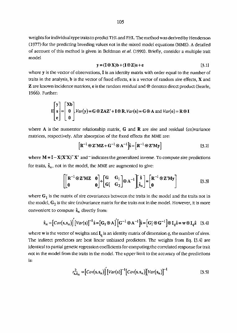
105
weights for individual type traits to predict THL and FHL. The method was derived by Henderson
(1977) for the predicting breeding values not in the mixed model equations (MME). A detailed
of account of this method is given in Boldman et al. (1990). Briefly, consider a multiple trait
model
y = (I®X)b + (I®Z)s+e B.l]
where y is the vector of observations, I is an identity matrix with order equal to the number of
traits in the analysis, b is the vector of fixed effects, s is a vector of random sire effects, X and
Z are known incidence matrices, e is the random residual and ® denotes direct product (Searle,
1966). Further:
, Var{y) = G ® ZAZ' +1 ® R, Var{s) = G ® A and Va/(e) = R ® I
where A is the numerator relationship matrix, G and R are sire and residual (co)variance
matrices, respectively. After absorption of the fixed effects the MME are:
y Xb' s = 0 e 0
R~^ ® Z'MZ + G"^ ® A"^ ]s = [r"^ ® Z'My] [3.2]
V^®Z'MZ 0 +
G Gi ®A"1 s "R~^®Z'My' 0 0 G'l G2. 0
where M = I - X(X'X) X and indicates the generalized inverse. To compute sire predictions
for traits, s„, not in the model, the MME are augmented to give:
[3.3]
where Gj is the matrix of sire covariances between the traits in the model and the traits not in
the model. Go is the sire (co)variance matrix for the traits not in the model. However, it is more
convenient to compute s„ directly from:
= [Cov(s.s„ )] [Vû/(s)]~^ s = [G, ® A]'[g-1 ® A"^ ]s = [g [ ® G"^ ]® I^s = w ® I^s [3.4]
where w is the vector of weights and Iq is an identity matrix of dimension q, the number of sires.
The indirect predictors are best linear unbiased predictors. The weights from Eq. [3.4] are
identical to partial genetic regression coefficients for computing the correlated response for trait
not in the model from the traits in the model. The upper limit to the accuracy of the predictions
is:
'à„ =[Cov(s.s„)] [Ms)] ^[Cov(s.s„)][Vfl/ (s„)] ' [3.5]

106
which would be possible if the predictors for the sire random effects in the model all had
accuracies of 1.00. Boldman et al. (1992) reported that the predictions FHL had upper limit
accuracy of 0.56. Also, it was shown that indirect selection for FHL would be more effective than
direct selection for FHL when the sire have less than 75 effective daughters.
Conclusions
In summary, the possibility for direct selection for longevity in dairy cattle will be limited
by the time required to accumulate sufficient data to accurately estimate sire breeding values.
Direct selection is also further hampered by low heritabilities on the observed scale. Several
studies have found a moderate to high genetic relationship among longevity and milk
production traits. These relationships appear partly due to voluntary culling for low production.
Therefore, there is need to redefine longevity in terms of involuntary culling if, longevity is to
be incorporated into dairy cattle breeding objectives. Genetic relationships between type and
longevity appear to exist in the populations studied. Several studies have used these
relationships to predict longevity. Measures of overall type appear to be of little value in
predicting longevity, however individual linear type traits provide a better basis for predicting
longevity. Much of work on longevity has be confined to the Holstein breed. This study will
investigate the genetics of THL and FHL, relationships among THL and FHL, and linear type and
first lactation milk production in Guernseys with the objective to deriving prediction equations
for indirect selection for 48 month THL and FHL. The second part of this study will apply linear
programming to Guernsey and Holstein herd life prediction equations for to identity which
linear traits optimize THL and FHL.

107
PAPER 3. ANALYSIS OF HERD LIFE IN GUERNSEY DAIRY CATTLE
Abstract
Heritabilities and genetic and phenotypic correlations for 48- and 72-mo herd life were
estimated from multiple-trait REML from sire models incorporating sire relationships. Two traits
were defined for 48- and 72-mo herd life, true herd life and functional herd life, which were
adjusted for milk production prior to culling. Heritabilities for 48- and 72-mo herd-life traits were
low, ranging from .02 to .07; genetic correlations among herd-life traits ranged from .82 to .95,
and phenotypic correlations ranged from .80 to .97. Genetic correlations between the herd-life
traits and first lactation milk, fat, and protein production ranged from .37 to .81. Genetic
correlations were lower between functional herd life and milk, fat, and protein production than
among true herd life and these same variables. Multiple-trait REML from sire models, which
included sire relationships, was used to estimate genetic and phenotypic correlations between
48-mo true or 48-mo functional herd life and linear type traits for registered Guernsey cattle. The
genetic correlations were used to compute weights for indirect prediction of true and functional
herd-life PTA from linear type traits PTA. The predictions are equivalent to multiple-trait BLUP
with no observations for herd life.
Introduction
Longevity, or a cow's productive life in a herd, has been measured in terms of several traits,
e.g., number of lactations, age at disposal, stayability, and survival scores (Dentine et ai, 1987;
Hogue and Hogdes, 1981; Hudson and Van Vleck, 1981; Madgwick and Goddard, 1989). The
economic importance of longevity has been well documented (Allaire and Cunningham, 1980;
Harris 1989; Renkema and Stelwagen, 1978; van Arendonk, 1985).
Direct selection for longevity in dairy cattle is limited by the time required to accumulate
sufficient data to estimate sire breeding values accurately (Smith and Quaas, 1984). Direct
selection is hampered further by low heritabilities on the observed scale (Dentine etal, 1987;
Hudson and Van Vleck, 1981). Several studies found moderate to high genetic relationships
between longevity and milk production traits (DeLorenzo and Everett, 1982; Dentine etal., 1987;
Everett etal., 1976; Hudson and Van Vleck, 1981, Van Doormal etal., 1986). These relationships
appear to be due partly to voluntary culling for low production. Therefore, if longevity is to be
incorporated into dairy cattle breeding objectives, the characteristic should be redefined in terms
of involuntary culling (Ducrocq etal., 1988a,b). Ducrocq etal. (1988a,b) defined two herd-life
traits: true herd life (THL), or total longevity, and functional herd life (FHL), a measure of herd
life when cows are subject to involuntary culling only. Genetic relationships between type and
longevity have been reported (Boldman etal., 1992; Rogers etal., 1989; Rogers etal., 1990;

108
Rogers et al., 1991b). Much of the work on longevity has been confined to the Holstein and jersey
breeds. The objectives of this study were 1) to investigate the genetics of THL and FHL and the
relationships among them, 2) to investigate linear type traits and first lactation milk production
in Guernsey cows, and 3) to derive prediction equations for indirect selection for 48-mo THL
and FHL.
Materials and methods
Herd life data
Production data were extracted from USDA Animal Improvement Program files. The records
consisted of registered and grade daughters of Guernsey sires that had left the herd or had an
opportunity to survive to 48 or 72 mo. The criteria given by Foster etal. (1989) and by Boldman
etal. (1992) were used to determine whether a cow had left the herd. Cows were assigned the
number of days that they remained in the herd from birth; if they were still in the herd at 48 or
72 mo, they were assigned a herd life of 1464 or 2196 d from birth, respectively. The 72-mo herd-
life data were a subset of the 48-mo data. Data for cows with an age at first calving greater than
40 mo were removed. All cows were required to have mature equivalent 305-d (ME305) records
for milk, fat, and protein production and to have sires with a US registration number. Milk, fat,
and protein production was used to compute a measure of FHL. Sires were required to have 10
or more progeny in two or more herds. Data consisted of 39,910 records on daughters of 563
sires for 48 mo and 21,453 records on daughters of 353 sires for 72 mo. The linear model for
THL analysis was:
+ gt + % + ^ijklm [1]
where yp/w 'S the record for THL on daughter m of sire / in group k, age at first calvingy, in herd
birth year /;
hyi is the fixed effect for herd birth year <;
Oj is the fixed effect for age at first calving j;
g;. is the fixed effect for genetic group k-
% is the random effect for sire / in genetic group k-, and
^ijklm's the random residual.
The relationship matrix included sires of the sires and maternal grandsires of the sires and
was computed from the method outlined by Quaas (1976). Sires of sires or maternal grandsires
with no production records and fewer than two relatives were excluded from the relationship
matrix. The sires were assigned to one of five genetic groups by birth year in 5-yr intervals; the

109
first interval was before or in 1965. Age at first calving was assigned in eight 60-d intervals; the
first parity interval was before or on 720 d.
Values for THL reflect both voluntary and involuntary culling. To estimate FHL, Ducrocq et
al. (1988b) used a cow's last lactation production prior to culling. In our study, linear and
quadratic covariables—a cow's standardized milk, fat, and protein production records—were
included in Model [1] to obtain a measure of FHL. Production records were standardized as
follows:
where is the standardization of production record for cow i, trait j (J = milk, fat, or protein)
in herd-year k ;
yijk is the last ME305 record for trait j of a cow / in herd-year k if the cow was culled
before 48- or 72-mo, or if the record began immediately before 48- or 72-mo of age and
the cow remained in the herd after 48- or 72-mo of age;
Xjk is the mean ME305 production of all cows in herd-year k for trait J; and
<5jk is the standard deviation for trait j in herd-year k.
For standardization of production records, at least 5 cows per herd-year were used to estimate
herd-year standard deviations (Hiedues et al., 1961).
Genetic and phenotypic covariances among 48-mo THL and FHL and 72-mo THL and FHL
were estimated using a multiple-trait model similar to Model [1], except that the effects were
nested within traits. Both 48- and 72-mo FHL were preadjusted for estimates of the linear and
quadratic covariables for standardized milk, fat, and protein production to obtain equal
incidence matrices so that a canonical transformation could be used for (co)variance estimation.
The preadjustment of THL to FHL was computed by means of:
where FHLijf^ is the FHL for cow i, trait j (J = milk, fat, or protein) in herd-year k-,
THLiji^ is the THL for cow /, trait j in herd-year k-,
Zjji- is the standardization of production record for cow /, trait J in herd-year k;
z is the mean of the standardization of production records;
Piy is estimate of the linear covariable for trait j; and

110
^2j is estimate of the quadratic covariabie for trait J.
Herd life and milk production
The 72-mo herd-life data were used to estimate genetic and phenotypic covariances among
herd-life traits; 48-mo THL, 48-mo FHL, 72-mo THL, and 72-mo FHL; and ME305 milk, fat, and
protein production. The 48- and 72-mo FHL measures were preadjusted separately for estimates
of linear and quadratic covariables for standardized milk, fat, and protein production. The JVIE305
milk, fat, and protein were preadjusted according to month of calving by the means of estimates
from a multiple-trait linear model: Model [1] reported by Harris et al. (1992). Preadjustment
facilitated the use of a canonical transformation in (co)variance estimation. The linear model for
multiple-trait analysis was:
ytijklm = hyti + + Stk + + ^lijklm f2]
where yiijkim 'S the record for trait t(.t= 1,..., 7) on daughter m of sire / in group k, age at first
calving j, in herd birth year i;
hy,i is the fixed effect for herd birth year / for trait t-,
a,j is the fixed effect for age at first calving j for trait t;
g,(. is the fixed effect for genetic group k for trait f;
s,i^l is the random effect for sire / in genetic group k for trait t- and
Ctijkini is the random residual.
The relationship matrix included sires of the sires and maternal grandsires of the sires. Sires of
sires or maternal grandsires with no records and fewer than two relationship ties were excluded
from the relationship matrix. The criteria for sire group and age at calving assignment were
identical to those applied in Model [1].
Herd-life and linear type trait data
Data from the American Guernsey Association linear type program were merged with 48-
and 72-mo herd-life data. Editing removed data for cows without a US registration number for
the sire. Cows were required to have all 15 linear type traits recorded and to have a stage of
lactation score within 0 to 350 when the traits were scored. For cows with multiple records for
type scores, only the first records were used. Sires were required to have 10 or more progeny
in at least two herds. Data from cows born before 1982 were discarded, because cows born
before that year that were culled early in their productive life may not have had the opportunity
to be type scored. Too few cows had the opportunity to survive 72 mo to permit analysis. Data
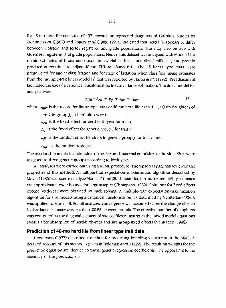
I l l
for 48-mo herd life consisted of 4571 records on registered daugthers of 124 sires. Studies by
Dentine et al. (1987) and Rogers et al. (1989, 1991a) indicated that herd life appears to differ
between Holstein and Jersey registered and grade populations. This may also be true with
Guernsey registered and grade populations. Hence, this dataset was analyzed with Model [1] to
obtain estimates of linear and quadratic covariables for standardized milk, fat, and protein
production required to adjust 48-mo THL to 48-mo FHL. The 15 linear type traits were
preadjusted for age at classification and for stage of lactation when classified, using estimates
from the multiple-trait linear Model [2] that was reported by Harris etal. (1992). Preadjustment
facilitated the use of a canonical transformation in (co)variance estimation. The linear model for
analysis was:
ytijkl = f^yti + Stj + ^tjk + ^tijkl B]
where is the record for linear type traits or 48-mo herd life f(f= 1,...,17) on daughter / of
sire k in group j, in herd birth year /;
hy,i is the fixed effect for herd birth year for trait t;
g,j is the fixed effect for genetic group j for trait /;
Sijk is the random effect for sire k in genetic group j for trait f; and
e,ijf^i is the random residual.
The relationship matrix included sires of the sires and maternal grandsires of the sires. Sires were
assigned to three genetic groups according to birth year.
All analyses were carried out using a REML procedure. Thompson (1982) has reviewed the
properties of this method. A multiple-trait expectation-maximization algorithm described by
Meyer (1986) was used to analyze Models [1] and [2]. The standard errors for heritability estimates
are approximate lower bounds for large samples (Thompson, 1982). Solutions for fixed effects
except herd-year were obtained by back solving. A multiple-trait expectation-maximization
algorithm for sire models using a canonical transformation, as described by VanRaden (1986),
was applied to Model [31. For all analyses, convergence was assumed when the change of each
(co)variance estimate was less than .001% between rounds. The effective number of daughters
was computed as the diagonal element of sire coefficient matrix in the mixed model equations
(MME) after absorption of herd-birth-year and sire group fixed effects (VanRaden, 1986).
Prediction of 48-mo herd life from linear type trait data
Henderson (1977) described a method for predicting breeding values not in the MME. A
detailed account of this method is given in Boldman et al. (1992). The resulting weights for the
prediction equation are identical to partial genetic regression coefficients. The upper limit to the
accuracy of the predictions is:
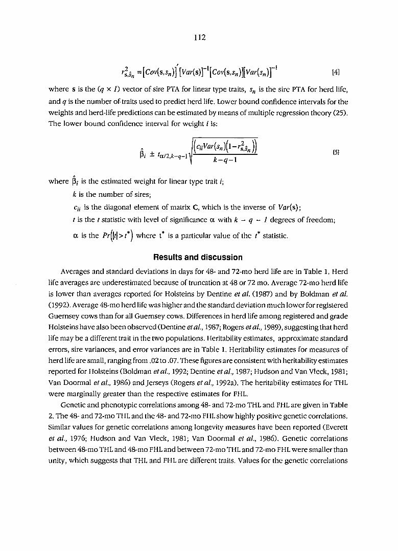
112
>is„ =[Cov(s.s„)] [Vflr(s)] '[Cov(s,j„)][Var(s^)] ^ [4]
where s is the (q x 7) vector of sire PTA for linear type traits, s„ is the sire PTA for herd life,
and <7 is the number of traits used to predict herd life. Lower bound confidence intervals for the
weights and herd-life predictions can be estimated by means of multiple regression theory (25).
The lower bound confidence interval for weight i is:
p,., jspa
where p; is the estimated weight for linear type trait /;
k is the number of sires;
c;; is the diagonal element of matrix C, which is the inverse of Var(s) ;
t is the t statistic with level of significance a with k - q - 1 degrees of freedom;
a is the where t* is a particular value of the t* statistic.
Results and discussion
Averages and standard deviations in days for 48- and 72-mo herd life are in Table 1. Herd
life averages are underestimated because of truncation at 48 or 72 mo. Average 72-mo herd life
is lower than averages reported for Holsteins by Dentine et al. (1987) and by Boldman et al.
(1992). Average 48-mo herd life was higher and the standard deviation much lower for registered
Guernsey cows than for all Guernsey cows. Differences in herd life among registered and grade
Holsteins have also been observed (Dentine et ai, 1987; Rogers et ai, 1989), suggesting that herd
life may be a different trait in the two populations. Heritability estimates, approximate standard
errors, sire variances, and error variances are in Table 1. Heritability estimates for measures of
herd life are small, ranging from .02 to .07. These figures are consistent with heritability estimates
reported for Holsteins (Boldman etal., 1992; Dentine etal., 1987; Hudson and Van Vleck, 1981;
Van Doormal etal., 1986) and Jerseys (Rogers etal., 1992a). The heritability estimates for THL
were marginally greater than the respective estimates for FHL.
Genetic and phenotypic correlations among 48- and 72-mo THL and FHL are given in Table
2. The 48- and 72-mo THL and the 48- and 72-mo FHL show highly positive genetic correlations.
Similar values for genetic correlations among longevity measures have been reported (Everett
et al., 1976; Hudson and Van Vleck, 1981; Van Doormal et al., 1986). Genetic correlations
between 48-mo THL and 48-mo FHL and between 72-mo THL and 72-mo FHL were smaller than
unity, which suggests that THL and FHL are different traits. Values for the genetic correlations
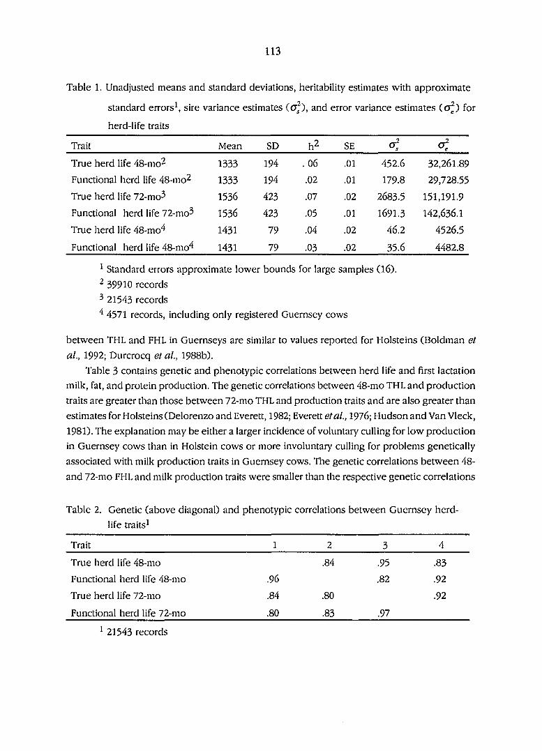
113
Table 1. Unadjusted means and standard deviations, heritability estimates with approximate
standard errors\ sire variance estimates ((T^), and error variance estimates (CT^) for
herd-life traits
Trait Mean SD h2 SE of
True herd life 48-mo2 1333 194 . 06 .01 452.6 32,261.89
Functional herd life 48-mo^ 1333 194 .02 .01 179.8 29,728.55
True herd life 72-mo3 1536 423 .07 .02 2683.5 151,191.9
Functional herd life 72-mo^ 1536 423 .05 .01 1691.3 142,636.1
True herd life 48-mo'^ 1431 79 .04 .02 46.2 4526.5
Functional herd life 48-mo4 1431 79 .03 .02 35.6 4482.8
^ Standard errors approximate lower bounds for large samples (16).
- 39910 records
^ 21543 records
4571 records, including only registered Guernsey cows
between THL and FHL in Guernseys are similar to values reported for Holsteins (Boldman et
al., 1992; Durcrocq et al., 1988b).
Table 3 contains genetic and phenotypic correlations between herd life and first lactation
milk, fat, and protein production. The genetic correlations between 48-mo THL and production
traits are greater than those between 72-mo THL and production traits and are also greater than
estimates for Holsteins (Delorenzo and Everett, 1982; Everett etal., 1976; Hudson and Van Vleck,
1981). The explanation may be either a larger incidence of voluntary culling for low production
in Guernsey cows than in Holstein cows or more involuntary culling for problems genetically
associated with milk production traits in Guernsey cows. The genetic correlations between 48-
and 72-mo FHL and milk production traits were smaller than the respective genetic correlations
Table 2. Genetic (above diagonal) and phenotypic correlations between Guernsey herd-
life traits^
Trait 1 2 3 4
True herd life 48-mo .84 .95 .83
Functional herd life 48-mo .96 .82 .92
True herd life 72-mo .84 .80 .92
Functional herd life 72-mo .80 .83 .97
^ 21543 records

114
Table 3. Phenotypic and genetic correlations between Guernsey herd life and production
traits^
Phenotypic correlations Genetic correlations
Trait Milk Fat Protein Milk Fat Protein
True herd life 48-mo .42 .41 .46 .74 .81 .80
Functional herd life 48-mo .30 .29 .40 .41 .50 .36
True herd life 72-mo .40 .40 .43 .60 .67 .68
Functional herd life 72-mo .30 .29 .30 .37 .41 .37
1 21,543 records.
Table 4. Phenotypic and genetic correlations between Guernsey type and herd life traits for
registered Guernsey cows^
Phenotypic correlations Genetic correlations
Trait 48-mo THL2 48-mo FHL^ 48-mo THL2 48-mo FHL 3
Stature -.05 -.06 -.62 -.69
Strength -.03 -.03 -.74 -.73
Dairy form .04 .01 .13 .02
Foot angle .03 .02 -.10 -.14
Rear legs side view -.02 -.01 .12 .16
Body depth -.02 -.02 -.32 -j5
Rump width -.04 -.04 -.35 -.40
Thurl width -.02 -.03 -.66 -.70
Fore udder attachment .03 .03 .30 .35
Rear udder height .06 .04 .08 .01
Rear udder width .04 .02 -.08 -.15
Udder depth .02 .03 .07 .04
Udder cleft .04 .03 .44 .41
Front teat placement .02 .01 .15 .11
Teat length -.04 -.04 -.55 -.57
^ 4571 records.
^ THL = True herd life.
^ FHL = Functional herd life.

115
between 48- and 72-mo THL and milk production traits. Although correcting herd life for milk
production traits reduced the dependency among herd life and first lactation milk production,
estimating FHL in this manner may still be a crude estimate of the true FHL.
Genetic and phenotypic correlations between 48-mo THL and FHL and linear type traits for
registered Guernsey cows are in Table 4. The phenotypic correlations between linear type traits
and 48-mo THL and FHL are small and close to zero. Values for phenotypic correlations between
linear type traits and herd life were similar for British Holstein Friesians (Brotherstone and Hill,
1990), for Holsteins (Boldman et al, 1992) and for Jerseys (Rogers et al., 1991b). The genetic
correlations are consistent in direction with the genetic correlations for Holsteins (Boldman et
al., 1992; Rogers et al., 1990) and Jerseys (Rogers et al, 1992b) but different in magnitude.
Stature, strength, thurl width, and teat length have moderate to high negative genetic
correlations with both 48-mo THL and 48-mo FHL. In contrast fore udder attachment and udder
cleft are moderately positively genetically correlated with 48-mo THL and FHL herd life.
Table 5. Weights for predicting true and functional herd life from Guernsey linear
type traits and 95% lower bound confidence intervals, (CI), for the weights
48-mo THLl 48-mo FHL 2
Trait Weight CI Weight CI
Stature -.409 .475 -1.321 .480
Strength -2.265 1.661 1.671 1.676
Dairy form 2.412 1.020 .841 1.030
Foot angle .584 .821 .226 ^28
Rear legs side view -1.001 .912 .746 .920
Body deptii .428 .461 -.792 .466
Rump width -.997 .478 -.542 X82
Thurl width -1.638 1.551 -2.153 1.565
Fore udder attachment .356 .757 .381 .764
Rear udder height -.814 1.144 1.717 1.154
Rear udder widtli .288 1.622 -.575 1.637
Udder depth .005 .686 -.608 ^92
Udder cleft .975 .116 1.074 .117
Front teat placement -.104 1.020 .266 1.029
Teat length .501 .807 -.473 .814
^ THL = true herd life
- FHL = functional herd life

116
Differences in magnitude of the genetic correlations between 48-mo THL and 48-mo FHL and
the linear type traits are similar to those between 72-mo THL and 72-mo FHL in Holsteins
(Boldman et al., 1992). The greatest genetic correlation differences occurred for dairyness, rear
udder height, and rear udder width, which are traits that Harris et al. (1992) found to have the
greatest genetic correlation with first lactation milk production traits.
The weights for predicting 48-mo THL and 48-mo FHL from linear type trait PTA and lower
bound confidence intervals for the weights are in Table 5. The lower bound confidence intervals
were computed from Equation [5]. The differences in weights between 48-mo THL and 48-mo
FHL reflect the differences observed among the genetic correlations between 48-mo THL and
48-mo FHL and the linear type traits in Table 4. The weights in Table 5 can be considered as
partial genetic regression coefficients, and, as such, individual weights are difficult to interpret.
All 15 weights must be used in the prediction equation, inasmuch as removal of linear type traits
from the prediction equation would change the values of the weights (Boldman et at., 1992).
Weights from Table 5 were used to compare sire PTA for 48-mo THL and 48-mo FHL from the
multiple-trait analysis. Model [3], with sire PTA that were calculated from linear type trait PTA.
The simple correlations between the sire PTA from the two methods were .989 and .995,
respectively. Figures 1 and 2 illustrate the relation between the sire transmitting abilities
computed from multiple-trait analysis and the weights for THL and for FHL, respectively. The
upper bound r- values for 48-mo THL and 48-mo FHL predictions, computed from Equation [4],
were both .99. The high upper bound r^ values can be attributed to moderate to high genetic
correlations between stature, strength, thud width, teat length, fore udder attachment, and udder
cleft and 48-mo THL and 48-mo FHL. The accuracy of THL and FHL predictions was greater than
Table 6. Direct and PTA, for true and functional herd life for five randomly chosen
sires
MM PTAI PTA 2
Effective number of daughters THL3 FHL^ THL3 FHL^
Sire 25 55.6 -4.23 -5.43 -5.30 -5.58
Sire 49 15.2 .35 1.31 -.10 .68
Sire 51 119.7 -3.89 -1.51 -4.06 -1.42
Sire 70 123 2.08 .89 1.99 .92
Sire 95 8.9 2.16 2.74 1.65 2.58
^MM PTA = PTA from multiple trait mixed model.
ZpTA = PTA computed from linear type trait PTA.
^THL = True herd life.
^FHL = Functional herd life.
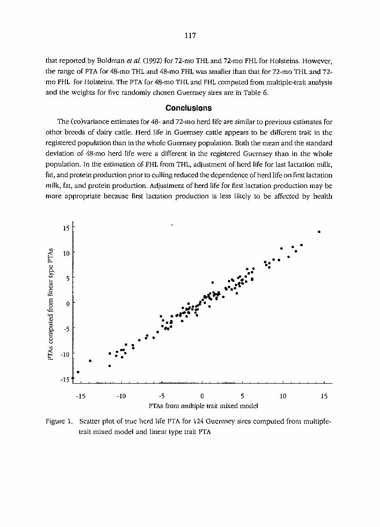
117
that reported by Boldman et al. (1992) for 72-mo THL and 72-mo FHL for Holsteins. However,
the range of PTA for 48-mo THL and 48-mo FHL was smaller than that for 72-mo THL and 72-
mo FHL for Holsteins. The PTA for 48-mo THL and FHL computed from multiple-trait analysis
and the weights for five randomly chosen Guernsey sires are in Table 6.
Conclusions
The (co)variance estimates for 48- and 72-mo herd life are similar to previous estimates for
other breeds of dairy cattle. Herd life in Guernsey cattle appears to be different trait in the
registered population than in the whole Guernsey population. Both the mean and the standard
deviation of 48-mo herd life were a different in the registered Guernsey than in the whole
population. In the estimation of FHL from THL, adjustment of herd life for last lactation milk,
fat, and protein production prior to culling reduced the dependence of herd life on first lactation
milk, fat, and protein production. Adjustment of herd life for first lactation production may be
more appropriate because first lactation production is less likely to be affected by health
15
10
-10
-15
-15
• • ••
• #
. ••
• ' XV. •
•a-®
. •
-10 -5 0 5
PTAs from multiple trait mixed model 10 15
Figure 1. Scatter plot of true herd life PTA for 124 Guernsey sires computed from multiple-
trait mixed model and linear type trait PTA

118
,r>f : r •
• •
-15 -10 10 -5 0 5
PTAs from multiple trait mixed model
Figure 2. Scatter plot of functional herd-life PTA for 124 Guernsey sires computed from
multiple-trait mixed model and linear type trait PTA
15
problems than last lactation production. However, the effectiveness of first lactation production
depends on the ability of first lactation production to predict production in later lactations when
voluntary culling occurs. Functional herd life should be used instead of THL in a selection index
for net profit because at least part of the effects of voluntary culling for milk production will be
reduced.
Genetic correlations between 48-mo THL and FHL and linear type traits in registered
Guernsey cattle were greater in magnitude than those in other breeds (Boldman et al., 1992;
Rogers et al., 1989). Methods for indirect prediction of transmitting abilities not in MME were
used to estimate transmitting abilities for 48-mo THL and 48-mo FHL from transmitting abilities
for linear type traits. The method had a high maximum accuracy for predicting transmitting
abilities for 48-mo THL and 48-mo FHL. This high accuracy can be attributed to the magnitude
of the genetic correlations among 48-mo THL and 48-mo FHL and linear type traits. Equations
for indirect prediction of transmitting abilities for THL and FHL are applicable only to registered
Guernsey cattle, which form the population from which genetic parameters were obtained.

119
Indirect prediction of herd life from linear type traits facilitates the modeling of the economic
value of linear type traits through their association with herd life. Moreover, the weights for
indirect prediction could be used to define the values for individual linear type traits optimizing
either THL or FHL. Genetic correlations among the linear type traits would need to be taken into
account within the optimization procedure.
Acknowledgements
The authors acknowledge K. Meyer for the use of her PK-REML FORTRAN 77 programs, P.
VanRaden for the use of his REMLD FORTRAN 77 program, and the Guernsey Foundation for
partial financial assistance.

120
PAPER 4. OPTIMIZATION OF LINEAR TYPE TRAITS FOR HERD LIFE
Abstract
Linear-programming models were developed to optimize the predicted transmitting abilities
(PTA) for 48-mo true herd life (THL) and functional herd life (FHL) in registered Guernsey cattle
and to optimize 72-mo THL and FHL in grade Holstein cattle by using linear-type traits. Also,
the linear-programming models were used to compute the change in optimal predicted herd life
from changes in individual linear type traits.
The optimal true and functional 48-mo herd-life PTA values for Guernseys were 18.22 and
17.81 days greater than mean PTA value for all Guernseys sires, respectively. The PTA values
for the linear-type traits that optimized 48-mo FHL had intermediate optima, except rear legs side
view and front teat placement. The PTA values for the linear-type traits that optimized 48 mo
THL all had intermediate optima. Strength, thurl width, and udder depth had a large effect on
the optimal THL and FHL 48-mo herd life in registered Guernseys.
The optimal taie and functional 72-mo herd-life PTA values for Holstein were 105.51 and
107.85 days greater than mean PTA value for all Holstein sires, respectively. Three linear-type
traits; suspensory ligament, disposition, and milkout, had optimal PTA values at the extreme
points for 72 mo FHL. All linear-type traits had intermediate optima PTA values for 72 mo THL.
The linear type traits; basic form, strength, stature, udder depth, and suspensory ligament were
found to have a large effect on both 72-mo THL and FHL herd life in grade Holsteins.
The optimal genotypes for FHL, with respect to linear-type PTA values, were not optimal
for THL in Holsteins or Guernseys.
Introduction
Fifty-point linear-type evaluation programs have been implemented by the Ayrshire, Brown
Swiss, Guernsey, Holstein, andjersey Breed Associations. Thompson etal. (1983) described the
advantages of using linear-type scores in preference to descriptive traits for animal evaluation.
Individual linear-type-trait evaluations are used by most breed associations and artificial
insemination organizations as a guide for selecting sires and mating cows. It is, therefore,
important to determine the associations among type traits and herd life. The relationship
between the individual linear-type-trait evaluations and herd-life evaluations will be of value
in selection and mating decisions.
Herd life, or length of productive life, is a trait of economic importance (Allaire and
Cunningham, 1980; Van Arendonk, 1985). Several studies have reported a moderate to high
positive genetic relationship between herd-life and milk-production traits. This relationship may
121
in part be due to voluntary culling for low production. Herd life can be redefined as two traits
(Ducrocq etal, 1988a,b): true herd life (THL), which is total longevity, and functional herd life
(FHL), which is a measure of herd life when a cow is only subject to involuntary culling. Genetic
and phenotypic relationships between linear type and herd life have been investigated in a
number of studies (Boldman et ai, 1992; Foster et ai, 1989; Harris et al., 1992b; Rogers et al.,
1989; Rogers etal., 1990,Rogers, etal., 1991). Recently, Boldman etal. (1992) and Harris etal.
(1992b) reported weights for predicting true and functional herd-life PTAs from linear-type-trait
predicted transmitting abilities (PTA) from Holstein and Guernsey cattle, respectively. These
weights can be used with optimization techniques such as linear programming (LP) to determine
the linear-type-trait PTA values that optimize herd life.
The objectives of this study were to determine the values of linear-type-trait PTA that
maximize THL and FHL PTAs in Holstein and Guernsey cattle and to investigate the optimal
relationships among individual linear-type-trait PTAs and herd-life PTA.
Linear type scores for 18 traits and 72-mo THL, and FHL from 53,830 grade Holstein cows
from 617 sires were previously analyzed by Boldman etal. (1992) by using a multiple-trait REML
algorithm. Weights to predict 72-mo THL and FHL from linear-type evaluations were computed.
Harris etal. (1992b) analyzed 15 linear-type scores, 48-mo THL, and FHL, from 4571 registered
Guernsey cows from 124 sires by using a multiple-trait REML sire model. Weights for predicting
48-mo THL and FHL from linear-type evaluations were computed by using the method described
in detail by Boldman et al. (1992). The predictions of herd life using the weights are equivalent
to multiple-trait BLUP evaluations in which herd life is included in the analysis with zero
observations (Boldman etal., 1992). The weights from Boldman etal. (1992) and Harris etal.
(1992b) are given in Table 1, with the upper bound accuracy for each of the predictions.
Four LP models were developed; grade Holstein 72-mo THL, grade Holstein 72-mo FHL,
registered Guernsey 48- mo THL, and registered Guernsey 48-mo FHL. A linear program has the
general form:
Materials and methods
max z = cjAi + C2X2 +• • • +c„.v„
5 . t . a , i A " ! + 0 , 2 ^ 2 + • • • = b i i = 1 ml
j = ml + l,...,m2
k = m2 + l w3
a^l-vi +aj2x2+- - -+a jnxn^b j
Xi>Q for alii / = ],...,/i
[1]
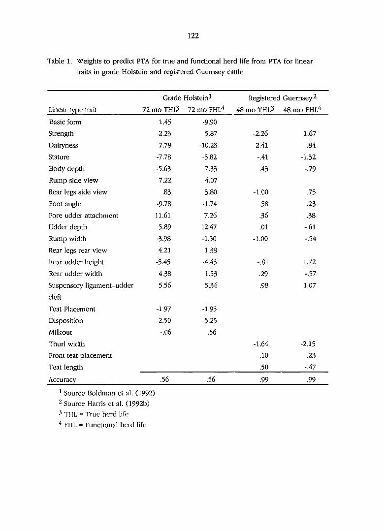
122
Table 1. Weights to predict PTA for true and functional herd life from PTA for linear
traits in grade Holstein and registered Guernsey cattle
Grade Holstein 1 Registered Guernsey 2
Linear type trait 72 mo THL? 72 mo FHl4 48 mo THL3 48 mo FHL4 Basic fomn 1.45 -9.90
Strength 2.23 5.87 -2.26 1.67
Dairyness 7.79 -10.23 2.41 .84
Stature -7.78 -5.82 -.41 -1.32
Body depth -5.63 7.33 .43 -.79
Rump side view 7.22 4.07
Rear legs side view .83 3.80 -1.00 .75
Foot angle -9.78 -1.74 .58 .23
Fore udder attachment 11.61 7.26 .36 .38
Udder deptli 5.89 12.47 .01 -.61
Rump width -3.98 -1.50 -1.00 -.54
Rear legs rear view 4.21 1.38
Rear udder height -5.45 -4.45 -.81 1.72
Rear udder width 4.38 1.53 .29 -.57
Suspensory ligament-udder 5.56 5.34 .98 1.07
cleft
Teat Placement -1.97 -1.95
Disposition 2.50 5.25
Milkout -.06 .56
Thurl width -1.64 -2.15
Front teat placement -.10 .23
Teat length .50 -.47
Accuracy .56 ^56 .99 .99^
^ Source Boldman et al. (1992)
- Source Harris et al. (1992b)
^ THL = True herd life
FHL = Functional herd life

123
where z is the objective function Cj is the ilh coefficient of the objective function, and
{Ax{<,=,>}b} is the set of constraints in which A is a matrix of constraint coefficients for the
vector of activities x and b is a vector of resources for the m3 constraints. For a complete
description of LP and methods for solving linear programs, see Sposito (1989). The weights given
in Table 1 form the basis of the objective functions for the four LP models, the c, s in Eq. [1].
The objective of the LP models was to determine the optimal values of the linear type-trait PTAs
ixis in Eq. [1]) that maximize the predicted herd life. There are two major requirements for
modeling herd-life prediction from linear type in an LP model. First is the placement of upper
and lower bounds on the linear-trait PTA so that they do not exceed the maximum or minimum
PTA obtained from the multiple-trait REML analyses. Second, the genetic covariance structure
among linear type-traits should be incorporated into the LP model.
The maximum and minimum PTA values were from the multiple-trait REML analyses
(Boldman etal., 1992; Harris etal., 1992b). These were used to compute upper and lower bound
constraints for each of the linear type-traits. The objective of developing constraints to mimic
the genetic covariances among linear type-traits, is to restrict the hyperspace of the LP models
to include only combinations of linear-type PTAs that are genetically feasible. Upper and lower
bounds that enclose the feasible region among any two linear-type traits were defined by using
contours of the bivariate normal-density function for linear type-traits with a genetic correlation
greater than 0.25 in absolute value. Genetic correlations of less than 0.25 in absolute value would
have upper and lower bounds defining the feasible region that were outside or close to the
bounds defining the maximum or minimum PTAs. A detailed account of this procedure is given
in Harris etal. (1992c) Appendix 1. The bivariate normal contours were computed by using the
upper 75% percentile of a chi-square distribution and genetic (co)variances obtained from the
multiple-trait analyses. Two constraints were computed parallel to the major axis of the contour
ellipse and tangent to the ellipse at the intersection of the minor axis and the contour line. Eight
further constraints were computed tangent to the contour ellipse at the intersection of four lines
parallel to the minor axis. The distances along the major axes from the intersection of the major
and minor axes for the four parallel lines were set to ±1/2 and ±1/3 of the length of the major
axis. The length of the major and minor axes can be computed from the eigenvectors and
eigenvalues of the genetic (co)variance matrix Qohnson and Wichern, 1988). A simplex-based
algorithm (Sposito, 1989) was used to solve the LP models. The simplex algorithm required the
A', s to be greater or equal to zero. Each linear type PTA was expressed as the difference between
two ,Y,- s in the LP model so that the s would be greater or equal to zero even though the PTA
can have either a positive or negative value. This doubled the number of variables in each model.
The two grade-Holstein LP models had a total of 462 variables (including slack variables) and

124
426 less than or equal constraints, and the two registered-Guernsey LP models had 490 variables
(including slack variables) and 460 less than or equal constraints.
The LP models were used to compute the change in optimal predicted herd life from a
change in an individual linear type-trait. An extra constraint was used, x, = X, where Xj is the /th
linear-type-trait PTA value and X is value of the restriction. This procedure simultaneously
accounts for changes in the other linear-type traits resulting from the restriction on the /th linear-
type-trait PTA by the incorporating the genetic covariances among the linear-type traits in the
LP models. The difference between the optimal herd life PTA with and without the restriction
is the total change in optimal herd life PTA. The optimal change in herd life cannot be obtained
from the weight for predicting herd life for the trait that is restricted because the restriction effects
the possible values that other correlated linear-type traits can have. This procedure, in concept,
maximizes the value of herd life by finding the optimum values for the linear-type traits that are
not restricted. This procedure is repeated for each trait over a range of values for X. The range
from the maximum to the minimum PTA was divided in to 50 divisions for each linear-type trait.
The value of X was set to the value of each division for each linear-type trait. This resulted in
900 linear programs for each of the grade-Holstein 72-mo THL and FHL models, and 750 linear
programs for each of the registered-Guernsey 48-mo THL and FHL models.
3
-3
- 2 - 1 0 1 2 PTA foot angle
Figure 1. The bounding constraints for foot angle and rear legs side view
(genetic correlation .34) used in the Holstein linear programming
models and PTA for 617 Holstein sires
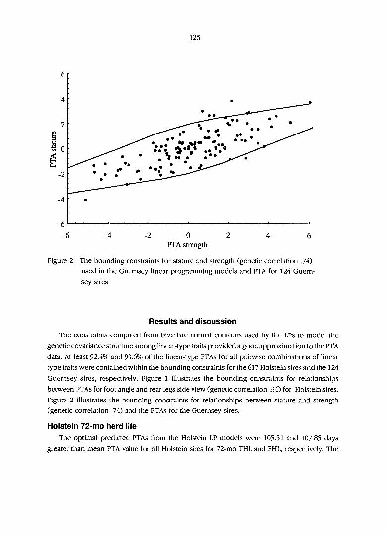
125
6
4
• • • •
2 •• • #* #* • •
• •• ** k 0 ••
• •
2
4
6 6 4 2 0 2 4 6
PTA strength
Figure 2. The bounding constraints for stature and strength (genetic correlation .74)
used in the Guernsey linear programming models and PTA for 124 Guern
sey sires
Results and discussion
The constraints computed from bivariate normal contours used by the LPs to model the
genetic covariance structure among linear-type traits provided a good approximation to the PTA
data. At least 92.4% and 90.6% of the linear-type PTAs for all pairwise combinations of linear
type traits were contained within the bounding constraints for the 617 Holstein sires and the 124
Guernsey sires, respectively. Figure 1 illustrates the bounding constraints for relationships
between PTAs for foot angle and rear legs side view (genetic correlation .34) for Holstein sires.
Figure 2 illustrates the bounding constraints for relationships between stature and strength
(genetic correlation .74) and the PTAs for the Guernsey sires.
Holstein 72-mo herd life The optimal predicted PTAs from the Holstein LP models were 105.51 and 107.85 days
greater than mean PTA value for all Holstein sires for 72-mo THL and FHL, respectively. The

126
Table 2. Optimal PTA for linear traits for predicting true and functional
herd-life PTA in grade holstein cattle
Linear type trait 72 mo THLI 72 mo FHL2
Basic form .06 -1.73
Strength .03 -.58
Dairyness 1.42 -.97
Stature -2.30 -1.09
Body depth -.65 1.13
Rump side view 2.23 2.33
Rear legs side view 1.54 1.24
Foot angle -.40 -.71
Fore udder attachment 1.66 1.29
Udder depth .23 1.24
Rump width -1.70 -1.84
Rear legs rear view 1.39 1.05
Rear udder height -.41 -.92
Rear udder width .63 .13
Suspensory ligament 1.63 1.94
Teat Placement 1.21 2.00
Disposition 2.50 2.53
Milkout 2.12 2.22
^ THL = True herd life
^ FHL = Functional herd life
optimal values are of similar magnitude as the values for 72-mo THL and FHL PTAs reported
by Boldman etal. (1992). The optimal PTAs for the linear traits are given in Table 2. Three linear
type-traits—suspensory ligament, disposition and milkout—had optimal values at the extreme
points, and rump side view had an optimal value close to an extreme point for FHL. All
linear-type traits had intermediate optimal PTA values for THL. But rump side view, rear legs
side view, disposition, and milkout had optimal values that were close to their respective
extreme points. The linear-type traits at, or close to, the extreme points for FHL were fast
milkout, extreme udder cleft, excellent disposition, and extreme slope to the rump when viewed

127
True 72 month herd life Functional 72 month herd life -80 -40 0 -40 -80 -80 -40 0 -40 -80
I ' I ' 1 ' I ' I I ' I ' I ' I ' I Basic Form I | • |
Strength I " I ' I
Dairyness . . *
Stature I "" ' I ' |
Body depth j """ ' [ [ " [ Rump side view | | | ' | Rear legs side view I ' I I • """ I
Foot angle I ' | | ;
Fore udder attachment i ' I i ' I
Udder depth j ' j j * j Rump width | ' | | ' |
Rear legs rear view ' '
Rear udder height | ^ I I ' i
Rear udder width I ' ^ I I ' I
Suspensory ligament , ' , . •
Teat placement I ' ' I | * ' I
Milkout I * j j * j Disposition i 1 | i * I i
Figure 3. The loss in predicted 72 month true (THL) and functional herd life (FHL) result
ing from changing PTA for individual linear type traits from their minimum
(left) to maximum value (right) and to a PTA value of zero (•) in grade Holstein
cattle
from the side. For THL, the linear-type traits close to the extreme points were for excellent
disposition, fast milkout, sickle-hocked rear legs when viewed from the side, and extreme slope
of rump when viewed from the side. The intermediate optima for udder depth, rump width, and
stature were found on the phenotypic scale by Foster et al. (1989) using linear and quadratic
regression coefficients. Foster etal. (1989) also found that the optimum for disposition was at
the extreme point. But optima for dairyness, milkout, and rear legs side view seem to be different
on the genetic scale compared with the phenotypic scale.
Comparing the optimal linear-type PTAs for maximizing THL and FHL, basic form, dairyness,
and body depth showed the largest differences. The differences in the weights used in the THL
and FHL objective functions (Table 1) also are greatest for these three traits, explaining the

128
• Functional herd life
True herd life
-3 -1 0 1
Udder depth PTA
Figure 4. Relationship between udder depth and true and functional
herd-life PTA in grade Holstein cattle
differences found in the optimal values. A sire with optimal linear type PTAs for FHL would have
a predicted PTA for THL of 68.18 days greater than the mean THL PTA value for all Holstein sires.
Also, a sire with optimal linear type PTAs for THL would have a predicted PTA for FHL of 52.24
days greater than mean FHL PTA value for all Holstein sires. Thus, genotypes that are optimal
for THL will not necessarily optimize FHL and vice-versa.
The effects of individual linear-type traits on optimal THL and FHL are illustrated in Figure
3. Figure 3 gives the reduction in days of herd life as a trait moves from its optimal value to either
its minimum or maximum value. Because the linear-programming models were optimized for
each change in a given linear-type trait PTA value, the reduction in days of herd life accounts
for changes in the optimal PTA values of the other 17 traits. As a result of simultaneously
accounting for the genetic covariances among the linear-type traits within the linear-program
ming model, it can be determined that traits such as rear legs side view, rump width, rear legs
rear view, and teat placement have little effect on the optimal THL and FHL herd life, whereas
basic form, strength, stature, udder depth, and suspensory ligament have a large effect on
72-mo THL and FHL. The ranges of the reduction in optimal herd life are similar for both THL

129
Table 3. Optimal PTA for linear traits for predicting true and functional
herd-life PTA in registered Guernsey cattle
Linear type trait 48 mo THLl 48 mo FHL2
Strength -2.07 -1.34
Dairyness 1.11 .76
Stature -2.31 -2.81
Body depth -.59 -2.13
Rear legs side view .70 2.02
Foot angle .22 -.01
Fore udder attachment 1.72 1.97
Udder depth 2.12 .03
Rump width -4.48 -3.25
Rear udder height -.98 1.16
Rear udder width .50 -.37
Thurl width -1.75 -2.01
Udder cleft 1.44 1.61
Front teat placement -1.99 2.69
Teat length .48 -2.41
and FHL. This is because both the THL and FHL LP models incorporate the genetic (co)variances
among the linear-type traits, which restricts the combinations of linear-type-trait PTAs to those
that are genetically feasible. The differences among the weights used in the objective functions
are reflected in the differences in the position of the optimal value and the position of the zero
PTA value in Figure 3. The shapes of the curves for the effect of individual type traits on optimal
herd life differ between THL and FHL, reflecting the differences in the weights used the objective
functions. This is illustrated for udder depth in Figure 4.
Guernsey 48-mo herd life The optimal predicted 48-mo THL and FHL PTAs were 18.22 and 17.81 days greater than
the mean PTA value for all Guernsey sires, respectively. The optimal predicted 48-mo THL and
FHL PTAs are of similar magnitude to 48-mo THL and FHL PTAs reported for Guernsey sires by
Harris et al. (1992b). The optimal PTAs for the linear traits are given in Table 3. Rear legs side
view and front-teat placement had optimal values at the extreme points, and udder cleft and
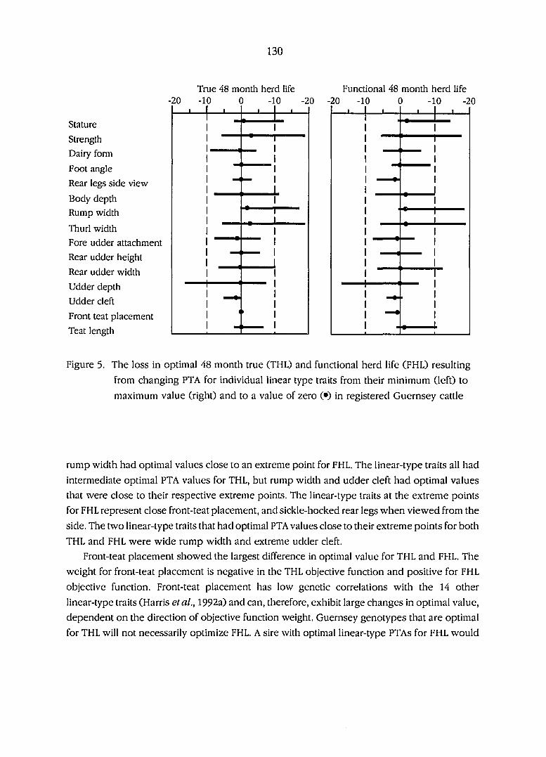
130
True 48 month herd life -20 -10 0 -10 -20
•
Stature
Strength
Dairy form
Foot angle
Rear legs side view
Body depth
Rump width
Thurl width
Fore udder attachment
Rear udder height
Rear udder width
Udder depth
Udder cleft
Front teat placement
Teat length
Functional 48 month herd life -20 -10 0 -10 -20
JL
Figure 5. The loss in optimal 48 month true (THL) and functional herd life (FHL) resulting
from changing PTA for individual linear type traits from their minimum (left) to
maximum value (right) and to a value of zero (•) in registered Guernsey cattle
rump width had optimal values close to an extreme point for FHL. The linear-type traits all had
intermediate optimal PTA values for THL, but rump width and udder cleft had optimal values
that were close to their respective extreme points. The linear-type traits at the extreme points
for FHL represent close front-teat placement, and sickle-hocked rear legs when viewed from the
side. The two linear-type traits that had optimal PTA values close to their extreme points for both
THL and FHL were wide rump width and extreme udder cleft.
Front-teat placement showed the largest difference in optimal value for THL and FHL. The
weight for front-teat placement is negative in the THL objective function and positive for FHL
objective function. Front-teat placement has low genetic correlations with the 14 other
linear-type traits (Harris etal., 1992a) and can, therefore, exhibit large changes in optimal value,
dependent on the direction of objective function weight. Guernsey genotypes that are optimal
for THL will not necessarily optimize FHL. A sire with optimal linear-type PTAs for FHL would
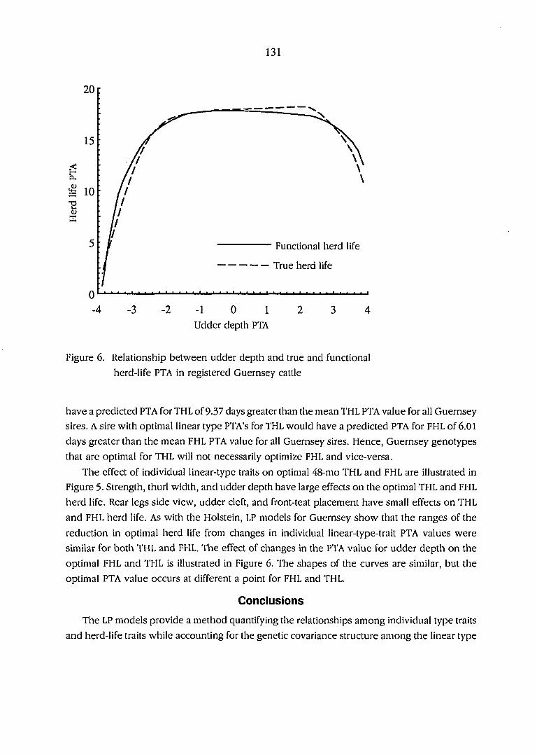
131
20
15
Ë "Ê 10
•§ x
0 -3 -2
Functional herd life
True herd life
-1 0 1
Udder depth PTA
Figure 6. Relationship between udder depth and true and functional
herd-life PTA in registered Guernsey cattle
have a predicted PTA for THL of 9.37 days greater than the mean THL PTA value for all Guernsey
sires. A sire with optimal linear type PTA's for THL would have a predicted PTA for FHL of 6.01
days greater than the mean FHL PTA value for all Guernsey sires. Hence, Guernsey genotypes
that are optimal for THL will not necessarily optimize FHL and vice-versa.
The effect of individual linear-type traits on optimal 48-mo THL and FHL are illustrated in
Figure 5. Strength, thurl width, and udder depth have large effects on the optimal THL and FHL
herd life. Rear legs side view, udder cleft, and front-teat placement have small effects on THL
and FHL herd life. As with the Holstein, LP models for Guernsey show that the ranges of the
reduction in optimal herd life from changes in individual linear-type-trait PTA values were
similar for both THL and FHL. The effect of changes in the PTA value for udder depth on the
optimal FHL and THL is illustrated in Figure 6. The shapes of the curves are similar, but the
optimal PTA value occurs at different a point for FHL and THL.
Conclusions
The LP models provide a method quantifying the relationships among individual type traits
and herd-life traits while accounting for the genetic covariance structure among the linear type
132
traits. Also, the LP models identify the optimal PTA values that maximize herd-life PTA. This is
a useful tool in providing information for selection and mating decisions involving linear type
traits.
The results from the LP models are applicable to the two populations that were studied;
grade Holsteins and registered Guernseys. Though two distinct populations were studied:
separately, there were similarities in the results. Three linear-type traits—strength, stature, and
udder depth—had large effects on optimal 72-mo THL and FHL in grade Holsteins and on
optimal 48-mo THL and FHL in registered Guernseys. Suspensory ligament or udder cleft was
optimal at or close to extreme cleft in all four LP models.
The optimal genotypes for FHL were not optimal for THL for Holsteins or Guernseys. This
is important when deciding which herd life measure to use in a selection program. The
milk-production traits are of primary importance in the selection of dairy cattle. Therefore, using
FHL in breeding objectives would be better than using THL because the influences of culling
low producing are removed, reducing the dependencies between herd life and milk-production
traits.
Acknowledgment
The authors acknowledge the Guernsey Foundation and 21st Century Genetics, Inc. for partial
financial assistance.

133
REFERENCES
Allaire, F. R., and E. P. Cunningham. 1980. Culling on low milk yield and its consequences for
the dairy herd. Livest. Prod. Set. 7:349.
Boldman K. B., A. E. Freeman, B. L. Harris, and A. L. Kuck. 1991. Prediction of sire for herd life
from transmitting abilities of linear type traits. J. Dairy Sci. (in press)
Brotherstone, S., and W. G. Hill, 1990. Dairy herd life in relation to type traits and production.
Proc. 4th World Congr. Genet. Appl. Livest. Prod., Edinburgh, UK, V:209.
Bulmer, M. G. 1981. Tlje mathematical theory of quantitative genetics. Oxford University Press,
Oxford UK.
Burnside, E. B. and, J. W. Wilton, 1970. Anatomical traits as they relate to productive utility./. Dairy
Sci. 46:157.
Burnside, E. B., A. E. McClintock, and K. Hammond. 1984. Type, production and longevity in dairy
cattle: A review. Anim. Breeding Abstr. 52:711.
Calo, L. L., and R. E. McDowell, L. D., Van Vleck, and P. D. Miller. 1973. Genetic aspects of beef
p r o d u c t i o n a m o n g H o l s t e i n F r i e s i a n p e d i g r e e s e l e c t e d f o r m i l k p r o d u c t i o n . 5 c / .
37:676.
DeLorenzo, M. A., and R. W. Everett, 1982. Relationships between milk and fat production, type
and stayability in Holstein sire evaluation./. Dairy Sci. 67:661.
DeLorenzo, M. A., and R. W. Everett. 1986. Prediction of sire effects for probability of survival to
a fixed age with logistic linear model. /. Daity Sci. 69:501.
Dempster, E. R., and I. M. Lerner. 1950. Heritability of threshold characters. Genetics. 25:212.
Dentine, M. R., B. T. McDaniel, and H. D. Norman 1987. Evaluation of sires for traits associated
with herd life in grade and registered Holstein cattle. /. Dairy Sci. 70:2623.
Dong, M. C., and L. D. Van Vleck, 1989. Estimates of genetic and environmental (co)variance for
first lactation milk yield, survival and calving interval./. Dairy. Sci. 72:678.
Ducrocq, V., R. L. Quaas, E.J. Pollack, and G. Casella, 1988a. Length of productive life of dairy
cows. 1. Justification of a weibull model. / Dairy Sci. 71:306l.
Ducrocq, V., R. L. Quaas, E.J. Pollack, and G. Casella, 1988b. Length of productive life of dairy
cows. 2. Variance component estimation and sire evaluation./. Dairy Sci. 71:3071.
Everett, R. W., J. R. Keown, and E. E. Clapp. 1976a. Relationships among type, production and
stayability in Holstein sire evaluation./. Daity Sci. 59:1505.
Everett, R. W.,J. R. Keown, and E. E. Clapp. 1976b. Production and stayability trends in Holstein
cattle. /. Dairy Sci. 59:1532.
Falconer, D. S. 1989. Introduction to quantitative genetics. Longman Scientific and Technical,
Longman Group UK LTD., Essex, U.K.
134
Foster, W. W., A. E. Freeman, P. J. Berger, and A. L. Kuck. 1989. Association of type traits scored
linearly with production and herd life of Holsteins. J. Dairy Sci. 72:2651.
Foulley, J. L., D. Gianola, and S. Im. 1990. Genetic evaluation for discrete polygenic traits in animal
breeding. In Advances in statistical methods for genetic improvement of livestock. Ed D.
Gianola and K. Hammond. Advanced Series in Agric. Sci. 18. Springier Verlag, Berlin.
Ghosh, M., and B. K. Sinha. 1980. On the robustness of least squares procedures in regression
models. / Multivariate Analysis. 10:332.
Gianola, D. and J. L. Foulley. 1983. Sire evaluation for order categorical data with a threshold
model. Genet. Sel. Evol. 15:201.
Gilmour, A. R., R. D.Anderson, and A. L. Rae. 1985. The analysis of binomial data by a generalized
linear mixed model. Biometrika 72:593.
Harris, B. L. 1986. Optimal cow replacement on New Zealand seasonal supply dairy farms. Proc.
N. Z. Soc. Anim. Prod. 48:243.
Harris, B. L. 1989. Heritability and economics of survival rate. New ZealandJ. Agrlc. Res. 32:359.
Harris, B. L, A. E. Freeman, and E. Metzger 1992a. Genetic and phenotypic parameters for type
and production in Guernsey dairy cows. /. Dairy. Sci. (accepted)
Harris, B. L., A. E. Freeman, and E. Metzger. 1992b. Analysis of herd life in Guernsey dairy cattle.
J. Dairy. Sci. 75:1147.
Harris, B. L, and A. E. Freeman. 1992c. Economic value of response from sire selection in dairy
cattle-A linear programming model. Agrlc. Systems (submitted)
Heidues, T., L. D. Van Vleck, and C. R. Henderson. 1961. Actual and expected accuracy of sire
proofs under the New York system of sampling bulls. Z. Tierz. Zûchtungbiol. 75:323.
Henderson, C. R. 1977. Best linear unbiased prediction of breeding values not in the model for
records. / Daity Sci. 60:783.
Honnette, J. E., W. E. Vinson, J. M. White, and R. H. Kliewer. 1981a. Contribution of descriptively
coded type traits to longevity of Holstein cows. /. Dai>y Sci. 63:807.
Honnette, J. E., W. E. Vinson, J. M. White, and R. H. Kliewer. 1981b. Prediction of herd life and
lifetime production from first lactation and individual type traits in Holstein cows. / Dairy
Sci. 63:816.
Hoque, M., and J. Hogdes. 1981. Lifetime production and longevity of cows related to their sires
breeding values. / Dair}> Sci. 64:158.
Hudson G. F. S., and L. D. Van Vleck. 1981. Relationships between production and stayability in
Holstein cattle. J Daily Sci. 64:2246.
Johnson, R. A, and D. W. Wichern. 1988. Applied multivariate statistical analysis. Prentice-Hall,
Inc., Englewood Cliffs, NJ.
Knott, M. On the minimum efficiency of least squares. Biometrika 62:129.

135
Madgwick P. A., and M. E. Goddard. 1989. Genetic and phenotypic parameters of longevity in
Australian dairy cattle. J Dairy Set. 72:2624.
Meyer, K. 1986. Restricted maximum likelihood to estimate genetic parameters—in practice. Proc.
3rd World Congr. Genet. Appl. Livest. Prod., Lincoln, Nebraska XII:454.
Norman, H. D., and L. D. Van Vleck. 1972. Type appraisal. III. Relationships of first lactation
production and lifetime performance. J. Dairy Sci. 57:1394.
Norman, H. D., R. L. Powell, J. R. Wright, B. G. Cassell, and R. E. Pearson. 1983. Relations of linear
functional type traits to lifetime performance of Ayrshires, Guernseys, and Jerseys./ Dairy
Sci. Suppl. 1. (Abstr) 68:234.
Quaas, R. L. 1976. Computing the diagonal elements and inverse of a large numerator relationship
matrix. Biometrics 32:949.
Renkema, J. A., and J. Stelwagen. 1978. Economic evaluation of replacement rates in dairy herds.
I. Reduction of replacement rates through improved health. Livest. Prod. Sci. 6:15.
Robertson, A., and I. M. Lerner. 1949. The heritability of all-or-none traits: viability of poultry.
Genetics 34:395.
Robertson A., and F. S. F. Baker. 1966. The correlation between first lactation milk production and
longevity in cattle. Anim. Prod. 8:241.
Rogers, G. W., B. T. Daniel, M. R. Dentine, and L. P.Johnson. 1988. Relationships among survival
rates. Predicted differences for yield and linear type traits. / Dairy Sci. 71:214.
Rogers, G. W., B. T. Daniel, M. R. Dentine, and H. D. Norman. 1989a. Relationships among proofs
for survival, culling and linear type measured in first and later lactations./. Dairy Sci. 72:528.
Rogers, G. W., B. T. Daniel, M. R. Dentine, and D. A. Funk. 1989b. Genetic correlations between
survival and linear type measured in first lactation. /. Dairy Sci. 72:523.
Rogers, G. W., M. R. Dentine, I. Miedema, and H. D. Norman. 1990. Relationships among non-
yield culling and linear type traits in Holsteins. Proc. 4tb World Congr. Genet. Appl. Livest.
Prod., Edinburgh, UK, V:213.
Rogers, G. W., G. L. Hargrove, J. B. Cooper, and H. D. Norman. 1991. Management and genetic
influences on survival in Jerseys. /. Dairy Sci. 74:279.
Rogers, G. W., G. L. Hargrove, J. B. Cooper, and E. P. Barton. 1991b. Relationships among survival
and linear type traits in Jerseys./. Dairy Sci. 74:286.
Schseffer, L. R., E. B. Burnside. 1974. Survival rates of tested daughters of sires in artificial
insemination. /. Dairy. Sci. 57:1394.
Searle, S. R. 1966. Matrix algebra for the biological sciences. John Wiley and Sons, Inc. New York.
Shannon, P. 1984. Analysis of threshold data governed by underlying normal distributions.
Research Bulletin No. 2. Farm Production Division. N. Z. Dairy Board.
136
Smith, S. P. 1990. Survival, endurance and censored observations in animal breeding. In Advances
instatistical metbodsforgenetic improvement of livestock. Ed D. Gianola and K. Hammond.
Advanced Series in Agric. Sci. 18. Springier Verlag, Berlin.
Smith, S. P., and R. L. Quaas. 1984. Productive lifespan of bull progeny groups: failure time
analysis. J. Dairy Sci. 67:2999.
Snedecor, G. W., and W. G. Cochran. 1989. Statistical Methods. Eighth edition. Iowa State
University Press, Ames, Iowa, USA.
Sposito. V. A. 1989. Linear programming with statistical applications. Iowa State University press,
Ames.
Thompson, J. R., K. L. Lee, A. E. Freeman, and L. P.Johnson. 1983. Evaluation of a linearized type
appraisal system for Holstein cattle. J. Dairy Sci. 66:325.
Thompson, R. 1982. Methods for estimation of genetic parameters. Proc. 2nd World Congr. Genet.
Appl. Livest. Prod., Madrid, SpainV:95.
Thompson, R. 1990. Generalized linear models applied to animal breeding. In Advances in
statistical methods for genetic improvement of livestock. Ed D. Gianola and K. Hammond.
Advanced Series in Agric. Sci. 18. Springier Verlag, Beriin.
Van Arendonk, J. A. M. 1985. Studies on the replacement policies in dairy cattle. II. Optimum
policy and influence of changes in production and prices. Livest. Prod. Sci. 13:101.
Van Arendonk, J. A. M. 1991. Use of profit equations to determine relative economic value of dairy
cattle herd life and production from field data. y. Dairy Sci. 74:1101.
Van Doormaal, B. J., E. B. Burnside, and L. R. Schaeffer. 1985. Estimation of genetic parameters
for stayability in Canadian Holsteins./ Dairy Sci. 68:1763.
Van Doormaal, B. J., E. B. Burnside, and L. R. Schaeffer. 1986. An analysis of the relationships
among stayability, production, and type in Canadian milk-recording programs./. Dairy Sci.
69:1823.
Van Raden, P. M. 1986. Computational strategies for estimation of variance components. Ph.d.
Diss., Iowa State Univ., Ames.VanVleck, L. D. 1964. First lactation performance and herd
Wïe. f. Dairy Set. 57:1394.
Wright, S. 1934a. Analysis of variability in number of digits in an inbred strain of guinea pigs.
Genetics 18:471.
Wright, S. 1934b. The results of crosses between inbred strains of guinea pigs, differing in number
of digits. Genetics 19:537.

137
GENERAL SUMMARY
Linear programming was applied to two areas of dairy cattle selection, namely, the derivation
of economic weights for production and non-production traits, and the maximization of herd
life predicted transmitting abilities from linear-type transmitting abilities.
The rates of response to selection that were possible from an artificial insemination progeny
testing scheme were required to model the economics of this response within a dairy farm
system. To enable this. Hill's response to selection with overlapping generations was extended
to account for multiple stage selection in both sexes and for situations where there are different
selection intensities in the four reproductive pathways. The response to selection in overlapping
generations when selection is conducted in stages was shown to have a limit as time tends to
infinity that was equal to the response to selection in discrete generations when selection is
conducted in stages. The multi-stage response to selection equations were used to compute the
cumulative response and the response to a single cycle of selection for a progeny testing scheme
which has two-stage selection of the males to breed future males and females. These results were
compared to a model which assumed that the single-stage selection model was appropriate. The
single-stage selection model over estimated the response to a single cycle of selection by 6%
and the cumulative response to selection over 20 years by 8%.
Multi-stage selection equations were used to model rates of response to selection for nine
traits. A linear programming model of a farm system was developed to estimate the economic
value of the response to selection. A procedure was developed for constructing a hyperspace
containing variables which were correlated and that allow both the trend of the relation and the
variation around that trend to be expressed as linear constraints. This confined the model to
consider rates of response to selection that were genetically feasible. The linear programming
model accounted for the gene-flow within the herd over time, and the time value of money. The
model contained constraints to formulate least cost rations in terms of metabolizable energy
requirements, digestible protein requirements, bounds on total roughage intake, and bounds
on the acid digestible fiber content. The linear programming model was used to compute
optimal rates of selection and economic weights for four planning horizons. The production
traits, milk, fat and protein, had optimal rates of response to selection close to the maximum
rates achievable from the multi-stage gene-flow model. The relative economic weights were
considerably greater for fat, milk and protein compared to the non-production traits. Of the non-
production traits, somatic cell had the largest relative economic weights in all planning horizons.
Application of linear programming to the derivation of economic weights has a number of
advantages. Optimization of net incomes requires that the animal, feed and financial resources
are used efficiently. Economic weights derived from models which do not optimize the resources
will underestimate the economic value of the genetic gain. Moreover, optimization of resource

138
allocation over time as production changes and/or when evaluating the effect of changes to the
rate of response to selection for individual trait in the computation of economic weights, may
partially account for changing marginal products. Modeling the response to selection using the
bounding constraints based on bivariate normal contours enabled the linear programming
model to consider the economics of all correlated traits simultaneously when optimizing the net
income. The usefulness of the bounding constraints is not restricted to modeling the response
to selection. These constraints can be used in any linear program to model the relationships
between correlated variables where the joint distribution of the two variables is approximately
bivariate normal. The use of linear programming models to derive economic weights is not
restricted to dairy cattle farm systems. This approach will be useful where selection involves
decisions concerning a number of economically important traits.
The genetics of herd life were investigated in Guernsey dairy cattle. Two herd life traits were
defined—true herd life (THL) and functional herd life (FHL). True herd life was the observed
herd life truncated at either 48 or 72-mo. Functional herd life was defined as a measure of herd
life when a cow was subject to involuntary culling only. Functional herd life was derived from
THL by adjusting THL by a cow's standardized production prior to removal from the herd.
Multiple trait restricted maximum likelihood estimation (REML) was used to estimate heritability
for 48- and 72-mo THL and FHL, and estimate genetic and phenotypic correlations among 48-
and 72-mo THL and FHL using a sire model with relationships. Heritability estimates were small
ranging from 0.02 to 0.07. The estimates were consistent with estimates reported for other breeds
of dairy cattle. Genetic correlations among 72-mo and 48-mo measures of herd life ranged from
.82 to .95 and the corresponding phenotypic correlations ranged from .80 to .97. The high genetic
and phenotypic correlations were expected due to the part-whole relation between 48-mo herd
life and 72-mo herd life.
Genetic and phenotypic correlations between first lactation milk, fat and protein yield and
herd life traits were estimated. Both the genetic and phenotypic correlations were greater
between 48-mo and 72-mo THL and the first lactation yields than between first lactation
production and 48-mo and 72-mo FHL. These results suggested that at least part of the
dependency between herd life and voluntary culling for low production had been removed by
adjusting THL for lactation yield prior to culling.
Genetic and phenotypic correlations between 15 linear-type scores and 48-mo THL and FHL
were estimated on a subset of the data which contained registered Guernsey dairy cattle. The
phenotypic correlations were low and close to zero, similar to estimates reported for other
breeds of dairy cattle. Stature, strength, thurl width and teat length were moderately to highly
negatively genetically correlated with both 48-mo THL and FHL. Whereas, fore udder attachment
and udder cleft were moderately to highly positively genetically correlated with both 48-mo THL
139
and FHL. The genetic covariances between the herd life traits and the linear-type traits were used
to estimate weights for indirect prediction of transmitting abilities (PTA) for 48-mo THL and FHL
from linear-type PTA. The predictions are best linear unbiased predictors (BLUP) with herd life
having zero observations in the mixed model equations. The prediction equations had a
maximum R-squared value of 0.99 which would be achieved if the linear-type trait PTAs are
essentially known without error.
Linear programming models were developed to optimize the predicted PTA for 48-mo THL
and FHL for registered Guernsey cattle, and to optimize the predicted PTA for 72-mo THL and
FHL for grade Holstein cattle. The weights for indirect prediction of herd life from linear-type
trait PTA formed the basis of the objective functions in the linear programming models. Lower
and upper bound constraints based on bivariate normal contours were computed using the
genetic covariance between pairs of linear-type traits. These constraints ensure that the linear
programming models choose combinations of linear-type PTA which are genetically feasible.
The optimal true and functional 72-mo herd-life PTA values for Holstein were 105.51 and
107.85 days greater than the mean PTA value for all Holstein sires, respectively. Three linear-
type traits—suspensory ligament, disposition and milkout—had optimal PTA values at the
extreme points for 72-mo FHL. All linear-type traits had intermediate optimal PTA values for 72-
mo THL. The linear-type traits; basic form, strength, stature, udder depth and suspensory
ligament were found to have a large effect on both 72-mo THL and FHL herd life in grade
Holsteins. The optimal true and functional 48-mo herd-life PTA values for Guernseys were 18.22
and 17.81 days greater than the mean PTA value for all Guernsey sires, respectively. The PTA
values for the linear-type traits which optimized 48-mo FHL had intermediate optima except rear
legs side view and front teat placement. The PTA values for the linear-type traits which optimized
48-mo THL all had intermediate optima. Strength, thurl width and udder depth were found to
have a large effect on the optimal THL and FHL 48-mo herd life in registered Guernseys. The
optimal genotypes for FHL were not optimal for THL for both Holsteins and Guernseys. This
is important when deciding which herd life measure to use in a selection program. The milk
production traits are of primary importance in the selection of dairy cattle. Therefore the use
of FHL in breeding objectives would be better than THL since the influences of culling low
producing are removed thereby reducing the dependencies between herd life and milk
production traits.
The LP models provide a method for quantifying the relationships among individual type
traits and herd life measures while accounting for the genetic covariance structure among the
linear-type traits. Also, the LP models identify the optimal PTA values that maximize herd life
PTA. Linear programming models are a useful tool in providing information for selection and
mating decisions involving linear-type traits.
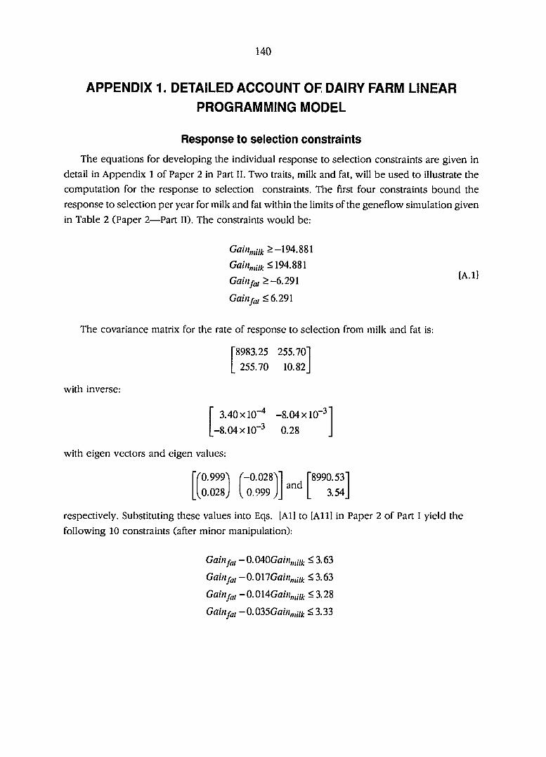
140
APPENDIX 1. DETAILED ACCOUNT OF DAIRY FARM LINEAR PROGRAMMING MODEL
Response to selection constraints
The equations for developing the individual response to selection constraints are given in
detail in Appendix 1 of Paper 2 in Part II. Two traits, milk and fat, will be used to illustrate the
computation for the response to selection constraints. The first four constraints bound the
response to selection per year for milk and fat within the limits of the geneflow simulation given
in Table 2 (Paper 2—Part II). The constraints would be:
> —194.881
Gain„,iii^ <194.881
Gain fa, >-6.291
Gain fat ^6.291
The covariance matrix for the rate of response to selection from milk and fat is:
with inverse:
8983.25 255.70"
255.70 10.82
3.40x10"^ -8.04x10"^
-8.04x10
with eigen vectors and eigen values:
,-3
r0.999"
0.028
-0.028
0.999
0.28
and 8990.53
3.54
respectively. Substituting these values into Eqs. [Al] to [All] in Paper 2 of Part I yield the
following 10 constraints (after minor manipulation):
Gain fa, -0.040Gain„,iif; < 3.63
Gain fa, — 0.0\lGain„,ni( ^ 3.63
Gain fa, — 0. OMGo/h^,///- < 3.28
Gain fa, -0.035Gain„,iii. < 3.33
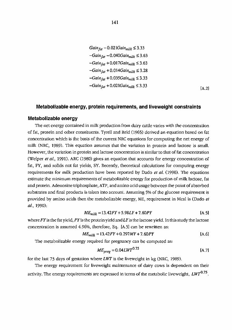
141
Gain fat ~0.02\Gain„iiii( < 3.33
—Gain— 0. Q^QGain^iHj^ < 3.63
—Gainj-(,i +0.017Ga/«„„7jt < 3.63
—Gainful + 0.< 3.28
—GainJ'ai +0.035Gain„,iif^ < 3.33
—Gainj^i +0.02lGain„iiii( < 3.33
Metabolizable energy, protein requirements, and liveweiglit constraints
Metabolizable energy The net energy contained in milk production from dairy cattle varies with the concentration
of fat, protein and other constituents. Tyrell and Reid (1965) derived an equation based on fat
concentration which is the basis of the current NRC equations for computing the net energy of
milk (NRC, 1989). This equation assumes that the variation in protein and lactose is small.
However, the variation in protein and lactose concentration is similar to that of fat concentration
(Welper etal., 1991). ARC (1980) gives an equation that accounts for energy concentration of
fat, FY, and solids not fat yields, SY. Recently, theoretical calculations for computing energy
requirements for milk production have been reported by Dado et al. (1990). The equations
estimate the minimum requirements of metabolizable energy for production of milk lactose, fat
and protein. Adenosine triphosphate, ATP, and amino acid usage between the point of absorbed
substrates and final products is taken into account. Assuming 5% of the glucose requirement is
provided by amino acids then the metabolizable energy, ME, requirement in Meal is (Dado et
al., 1990):
ME„,iik=l3.42FY + 5.9SLY + 1.60PY [A.51
where f y is the fat yield, PY is the protein yield and LY is the lactose yield. In this study the lactose
concentration is assumed 4.96%, therefore, Eq. [A.5] can be rewritten as:
ME„,iik = 1142FY + 0.291 MY + 7.60 PY [A.6]
The metabolizable energy required for pregnancy can be computed as:
MEpreg=0.04LWT^-'^^ [A.7]
for the last 73 days of gestation where LWT is the liveweight in kg (NRC, 1989).
The energy requirement for liveweight maintenance of dairy cows is dependent on their
activity. The energy requirements are expressed in terms of the metabolic liveweight, LWT^'^^.

142
The equations for metabolizabie energy requirements in Meal by parity for lactating cows are
(NRC, 1989):
parity 1 ME„,ain=^.\mLWr^-'^^ [A.8]
parity 2 = 0.1467LVV7'®-''^ [A.9]
parity 3+ =0.1333LWr°-''5 [A. 10]
and for dry cows, which are less efficient in energy utilization than milking cows, are (NRC, 1989):
parity 1 =0.2043LHT°-'^^ [A.ll]
parity 2 =0.1873LVy7'°-''^ [A.12]
parity 3+ =0.1702LVV7°-''^ [A.13]
The net energy content of liveweight tissue lost during lactation is 6.00 Mcal/kg (NRC, 1989).
The net energy from tissue loss is used with approximately 82% efficiency (ARC, 1980) resulting
in 4.92 Meal of metabolizabie energy per kilogram of tissue lost during lactation giving the
metabolizabie energy in Mcal/kg of tissue lost as:
MEioss=^.92LWL [A. 14]
where lwl is kg of tissue lost.
The metabolizabie energy required for liveweight gain in dairy cattle is computed from NRC
(1989) equations assuming an efficiency of metabolizabie energy of 0.60 and 0.47 for lactating
and dry dairy cows, respectively, as:
lactating = 0.0583LWT° +1.7LWG [A.15]
dry cows =0.0744LW° +2.11WG [A.16]
where lwg is the liveweight gain per day in kilograms.
Protein Requirements Both, ARC (1980) and NRC (1989) have developed similar schemes for computing dietary
protein requirements. ARC (1980) provides a greater emphasis on the need to consider separately
the nitrogen requirements of the mircobial population and the host animal in relation to energy
intake. This study will concentrate on the requirements for rumen digestible proteins (RDP)
assuming the supply of undegraded dietary protein (UDP) from the feedstuff meets the animals
demand for (UDP). This is not unreasonable given that the protein in most commercial feeds is
on average 60% digestible resulting 40% of the total protein being UDP.
The RDP requirement in kilograms for pregnancy, liveweight gain, loss and maintenance,
is calculated from the metabolizabie energy requirements using the ARC (1980)
recommendations as:
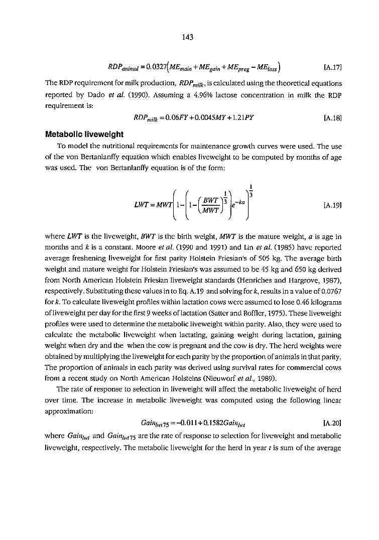
143
R D P ^ f f i m a l ^ ^ g a i n " ^ ^ p r e g ^ ^ l o s s ^ [ A . 1 7 ]
The RDP requirement for milk production, RDP„,jii,, is calculated using the theoretical equations
reported by Dado et al. (1990). Assuming a 4.96% lactose concentration in milk the RDP
requirement is:
RDP„,i,k=OMFY + Q.mSMY -^-X.llPY [A. 18]
Metabolic liveweight To model the nutritional requirements for maintenance growth curves were used. The use
of the von Bertanlanffy equation which enables liveweight to be computed by months of age
was used. The von Bertanlanffy equation is of the form:
1
f f \
LWT = MWT 1- 1 [JMRRJ
\ J J
where LWT is the liveweight, BV/T is the birth weight, MWT is the mature weight, a is age in
months and A is a constant. Moore et al. (1990 and 1991) and Lin et al. (1985) have reported
average freshening liveweight for first parity Holstein Friesian's of 505 kg. The average birth
weight and mature weight for Holstein Friesian's was assumed to be 45 kg and 650 kg derived
from North American Holstein Friesian liveweight standards (Henriches and Hargrove, 1987),
respectively. Substituting these values in to Eq. A. 19 and solving for k, results in a value of 0.0767
for k.To calculate liveweight profiles within lactation cows were assumed to lose 0.46 kilograms
of liveweight per day for the first 9 weeks of lactation (Satter and Roffler, 1975). These liveweight
profiles were used to determine the metabolic liveweight within parity. Also, they were used to
calculate the metabolic liveweight when lactating, gaining weight during lactation, gaining
weight when dry and the when the cow is pregnant and the cow is dry. The herd weights were
obtained by multiplying the liveweight for each parity by the proportion of animals in that parity.
The proportion of animals in each parity was derived using survival rates for commercial cows
from a recent study on North American Holsteins (Nieuworf et al., 1989).
The rate of response to selection in liveweight will affect the metabolic liveweight of herd
over time. The increase in metabolic liveweight was computed using the following linear
approximation:
= —0.011 + 0.[A.20]
where and are the rate of response to selection for liveweight and metabolic
liveweight, respectively. The metabolic liveweight for the herd in year t is sum of the average

144
cow metabolic live weight at year 0 and the gain for metabolic liveweight. The total metabolic
liveweight for the herd in year t is:
LWT^-''^ = +GF, •Gain,y,n5)Herdsize, [A.21]
where LWrf'^^ is the herd liveweight in year t, GF, is the gene flow parameter, is the
average cow metabolic liveweight at year 0 and Herdsize, is the size of herd in year t. The gene
flow parameter accounts for the expression of the response to selection through the herd over
time. The geneflow parameter for a given year is the sum across parities of the number of times
the response to selection is expressed in cows of a given parity multiplied by the proportion
of cows in that parity. The values for the gene flow parameter are given in Appendix 2. Increases
or decreases in the response to selection for herd life will affect the size of expression of response
to selection for in a given year by changing proportion of cows in each parity. The average herd
life of cows in year t with zero response to selection for herd life is:
7
Herdlife, = V [Survivali • Age, ) + Age^ [A.22] i=2
where Suiyivali is survival from parity / -1 to parity i and AgCi is the age of the cow at the start
of parity i in days. Assuming that an increase (decrease) in days of herd life would increase
(decrease) the probability of survival to each parity evenly, then one sixth of the response to
selection will contribute to the survival from parity i-1 to parity i. Therefore, the equation for herd
life in year t, accounting for response to selection for herd life is:
7
Herdlife, = {^Survivali , • Agei) + Agei [A.23] i=2
where Survivali , is the survival to parity / in year t:
^ [A.241 6agei
and Gahificrdiife's the rate of response to selection for herd life. The proportion of cows in each
parity in year t can be calculated from Survivalj, as:
IA.25I
^suiyivali, 1=2

145
where 7t/, is the proportion of cows in parity i in year t. To estimate for the rate of response
to selection for herd life was computed from the indirect response from selection in linear type
traits (Boldman et ai, 1992). Eq. [A.21] can be modified to account for the effect of herd life:
LWr^-^^-\pFt •Gainiyji'j^-^tGaini^g^^iife^-Herdsizet = IwtQ^^ • Herdsizci [A.26]
where is change in the metabolic liveweight in year t per unit change herd life. The values
for P, are computed directly from %i ,, and are given in Appendix 2.
Young stock rearing requirements To calculate the rearing costs of replacement females entering the herd, Eq. [A.19] was used
to compute the liveweight profile of the replacements. From this profile the metabolizable energy
for liveweight gain by month was calculated using Eq. [A.161. The metabolizable energy
requirement for maintenance was calculated from the following equation derived from (NRC,
1989) assuming an efficiency of metabolizable energy utilization of 0.47:
ME„,ain = 0.1[A.27]
The total energy requirement for rearing a replacement heifer is the maintenance and liveweight
gain requirements summed over 24 months (2 years of age). The total dietary protein
requirements is the total metabolizable energy requirement multiplied by 0.0327 (ARC, 1981).
Genetic change in herd life and liveweight will effect the requirements for replacement
females by changing the liveweight profiles or by changing the numbers of replacements reared.
The change in metabolizable energy requirements due to a change in response to selection for
liveweight, (p,, is the difference between the total metabolizable energy requirements
accounting for the response to selection less the total metabolizable energy requirement with
zero response to selection for liveweight, expressed per unit kilogram. These values were
computed for years 1 to 20 and are given in Appendix 2. The change in protein requirements
can be calculated directly from the change in metabolizable energy requirement per unit
kilogram response to selection multiplied by 0.0327 (ARC, 1981).
To account for the effects of response to selection for herd life on the number of heifers reared
it was assumed that an increase (decrease) in days of herd life would increase (decrease) the
probability of survival from parity / to parity / + 1 equally. A change in survival in year f will change
the proportions of heifers reared in years r-1 and t -2, since the heifers are reared over 24 month
period. With zero response to selection for herd life the proportion of rising 1 year old heifers
and rising 2 year old heifers reared in any one year would be 0.2808. The change in total
metabolizable energy requirements of replacements in year t, 6,, expressed per day herd life
is:
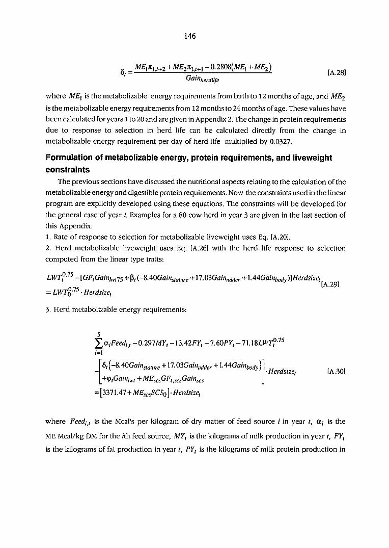
146
ô, = ~0. 2808(A/£j + MEi2^
GaiHiigrdUfe [A.28]
where ME^ is the metabolizable energy requirements from birth to 12 months of age, and ME2
is the metabolizable energy requirements from 12 months to 24 months of age. These values have
been calculated for years 1 to 20 and are given in Appendix 2. The change in protein requirements
due to response to selection in herd life can be calculated directly from the change in
metabolizable energy requirement per day of herd life multiplied by 0.0327.
Formulation of metabolizable energy, protein requirements, and liveweight constraints
The previous sections have discussed the nutritional aspects relating to the calculation of the
metabolizable energy and digestible protein requirements. Now the constraints used in the linear
program are explicitly developed using these equations. The constraints will be developed for
the general case of year t. Examples for a 80 cow herd in year 3 are given in the last section of
this Appendix.
1. Rate of response to selection for metabolizable liveweight uses Eq. [A.20].
2. Herd metabolizable liveweight uses Eq. [A.26] with the herd life response to selection
computed from the linear type traits:
^^0.75 _ + p, {-^AOGainstature + + \AAGainijoci^)]Herdsizet
0 75 = LWT^-^^ • Herclsize,
3. Herd metabolizable energy requirements:
5 ^UiFeedij -0.291 MY,-13A2FY,-IMPYt-lUSLWrj^-'^^ 1=1
ô j 8 . + 1 7 . 0 3 G c i i i i , i ^ ^ g i , + 1 . j Herdsize, [A.30]
+ ^scsG^t ,scsG^i^^scs
= [3371.47 + • Herdsize,
where Feedi , is the Meal's per kilogram of dry matter of feed source / in year t, a, is the
ME Mcal/kg DM for the ith feed source, MY, is the kilograms of milk production in year t, FY,
is the kilograms of fat production in year t, PY, is the kilograms of milk protein production in

147
year t, Gainées is rate of response to selection for somatic cell score, GFi g^s is the geneflow
parameter for the response to selection for somatic cell score in year t, ME^^s is metabolizable
energy content of the milk production discarded from increases in response to selection for
somatic cell count, SCSq is somatic cell score for herd at year 0. The value of 71.18 in the
constraint is computed from the coefficients for in Eq.'s [A.8] to [A. 17] weighted by the
proportion of cows in each parity. The value of 3371.47 is computed from metabolizable energy
for liveweight and loss during lactation and the rearing requirements, Eqs. [A. 15] to [A. 17] and
[A.26]. The values for a, are given in Appendix 2.
4. Digestible protein requirements:
5
^ViFeedij -0.045A/y, -O.Oôfy, -l.2\PY,-P,csGF,^,csfferdsize, -/=!
(9, (-8. OGaiiisiature +17. iOGaiitudder + IMGaiUhody ) + ^Herdsize, 0.0327 [A.31 ]
-71.1 %LWTf-'^^ 0.0327 > 0.0327(3371.47 + ME^^^SCSq )
where is the digestible protein requirement of discarded milk, V; is the kilograms of
digestible protein per kilogram dry matter for the /th feed source in year t. The values for D, are
given in Appendix 2.
5. Alfalfa hay and meal feed restriction:
Feedy +Feed2j -0.40^0.1 IGF,+4.SlGF,Gainfiji
+2.16GF,Gainpro, + 29.33GF,Ga//!/jy,75 + ME^csGFi^scs^^i'hcs )Herdsizei [A.32]
< Restrictioiiaifaifa
where RestrictioHaifaifa is the 40% restriction. Tlie coefficients for the rates of response to
selection for milk, fat, protein, somatic cell score and metabolic liveweight are included in
constraint to account for the change in the total consumed dry matter caused by response to
selection.

148
6. Acid free detergent (ADF) fiber constraints:
5
''^^iFeedii —0.25^0.1 + A.^lGF/GQin + 1=1
2. lôGFtGaitiprot +29.33GF,Gainiy^,-j^ + ME^cs^F,scsGainscs)Herdsizet
< Restnction25/[DF [A.33]
and:
5
"^^^ifeedii —0.l9{0.llgfigaiii„,iii^ +a.%lgffgaiiij-^ ;=1
+2. lèGFiGaiUprot + 29. SSGFjGa/zî/^^, 75 + ME^^fiFtscs^ainscs Herdsize, [A.34]
> Restrictioni^/[[)p
where is the proportion of ADF in the feed source, Restriction\^/^[)f and RestrictionisADF ^ce
the 19% and 25% ADF restrictions, respectively. The values for are given in Appendix 2.
Milk production, somatic cell score and mastitis constraints
The milk production in a given year will depend on the rates of response to selection for
production, somatic cell score (SCS), days open and herd life. The constraints is milk production
in year t is:
MYf — [G/^„„7/; jGa//!„„7^. + (—8.+ 17.03GciiHiij^gf
+1.44gainijgijy j+sg(.gigoiiig(^g + df ffiuhgaiuddy^opgfi J • h et dsizcf [A.34]
= myQ • Herdsize,
where GF„,iif;j is the geneflow parameter for milk yield, myQ average per cow milk yield in year
0, S^csj' d, mille are the change in the/th production trait from a unit change in
response to selection for herd life, SCS and days open, respectively. The constraints for fat and
protein yield are of the same form as Eq. [A.34].
The effects of changes in response to selection for herd life on milk production were
modelled using Eqs. [A.23] and [A.25] by computing the change in milk production resulting from
a change in herd life via of the changes to the age distribution accounting for conversion from

149
mature equivalent to actual production. The values for hijat. and h, protein are given in
Appendix 2.
The response to selection for milk, fat and protein yields are expressed in terms of mature
equivalent production, standardized for age, breed, region and month of calving. The geneflow
parameters for production were calculated including the conversion from mature equivalent to
actual production. The values for the geneflow parameters for milk, fat, and protein yield are
given in Appendix 2.
The effect of days open was to change the flow of milk production over time. As days open
increase (decrease), the time between the current and subsequent lactation will increase
(decrease). Compared to the situation constant days open the production from the herd will be
produced over a longer period of time reducing the production per day from the herd. To model
the changes in milk production from changes days open, lactation yields over time for milk,
fat and protein were computed using lactation curves from Schutz etal., (1990). It was assumed
that cows calved in equal proportions in each month of the year. The value for was
computed as the change in herd milk yield per day change in days open for year t. The values
for di^niiiic, d,jat and dt,protein are given in Appendix 2.
Dabdoub and Shook (1984) have quantified the loss in milk yield per increase in SCS.
Regression coefficients for a unit increase in SCS were -281+129 lb (127.5 kg) of milk for
lactations. Assuming cows in lactations 1 on average have the milk yield reduced by 281 lb then
the reduction in milk production from response to selection in SCS in year t, is:
,127.5 [A3.35]
where , is the geneflow parameter for SCS in year t. The geneflow parameter accounts for
the number of times the response to selection is expressed in year t and the age adjustment for
increases in SCS with increasing age. The increase in SCS with age has been reported by Wiggans
and Shook (1988). These results were to compute age adjustments for SCS. The adjustments were
computed as the ratio of the mean SCS for /th parity over SCS for first parity, since the response
to selection for SCS is in terms of first parity SCS. Values for fat and protein were computed from
Eq. [A3.35] assuming on average that a 1 kg loss of milk yield would result in a 0.036 kg loss in
fat yield and a 0.032 kg loss in protein. The values for andGF^^ , are given in Appendix
2.
Changes in the response to selection for somatic cell score could result in changes in the
incidence of mastitis. Dabdoub and Shook (1982) quantified a logistic relationship between SCS
and incidence of mastitis. The model equations were:

150
y = -4.10 + 1.145C5 [A.36]
and:
P = [A.37]
where p is the proportion of cows treated for mastitis. The use of this relationship allows the
cost of mastitis treatment from genetic change in SCS to be modeled. Equation [A.36] and [A.37]
can be approximated by a linear equation:
p = -0.3913 + 0.24895C5 [A.38]
which is used to formulate a linear program constraint for mastitis incidence:
Mast, -(0.2A^9GFg^g ,Gains(.s)He>'dsize(
= (-0.3913 + 0.24895C5o )Herdsize, [A.39]
where Mast, is number of mastitis cases treated in year t.
Salvage value and calf value constraints
The amount of salvage beef production and the numbers of calves will be effected by the
response to selection for herd life. Increases in herd life will decrease the culling rate reducing
the income from cull cows and reduce the replacement rate increasing the numbers of surplus
calves. The effect of changes in the response to selection for herd life was modeled using Eqs.
[A.23] and [A.25]. The constraint for salvage beef production in year t is:
Salvage, / dress - [Uherdlife.t +17.03Ga//;„^^g^ . [A.40]
+\MGambody )+T,Gaini^vt J = salvageo • Per salvage ' Herdsize
where Salvage, is the kg of beef sold for the herd in year t from cull cows, salvageQ is the average
kg of beef sold per cow in year 0, dress is the average dressing percentage, UherdUfej 'S the effect
of response to selection for herd life on salvage beef production in year t, Per^^lvage 'S percent
of the beef production from cull cows which is salvageable, and T, the effect of response to
selection for live weight on the salvage beef production per cow in year t. The values for T, were
calculated as the change in salvage value per cow from a unit increase in response to selection
for liveweight. Account was taken of the number of expressions of the response to selection in
a given year and the liveweight profiles across parities using Eq. [A. 19]. The values for UherdUfej

151
and Tf are given in Appendix 2.
The constraint for number of calf sales in year t is:
Calf t-Survcalf-
\^Cherdlife,t ("S- OGaiHsiature +17.3)QGain„jder + ^HerdsizCt [A.41]
= calfQ • Herdsize, -Surv^alf
where Calf, is the number of calves sold in year t, is the calfo average number of calves sold
per cow in year 0, Siaycaif is the percent of calves survival, and Ci,erdlife,t 'S the effect of response
to selection for herd life on proportion of calves sold in year . The values for Ci^erdlife^t are given
in Appendix 2.
Cashflow constraints
The constraint for fixed costs simply sets the fixed costs to a predefined value for each year.
Variable costs refer to the costs per cow such as breeding costs, housing costs, and labor, not
costs due to feeding, and treatment of mastitis. The constraint for variable costs per cow in year
t is:
VCf = vc, • Herdsize, [A.42]
where VC, is the variable cost for the herd in year rand vc, is the per cow variable cost in year
t.
The cashflow constraints compute the surplus or deficit in cash returns in year t accounting
for the accrual of the surplus or deficit over time and the time value of money. The cash flow
constraint in year 1 is:
Surptusi - Deficiti - MP^ • - FP\ • FY\ - PPi • PY^
5 Feedi iCfeedi i + MastiCmast\ - SalvaseiPrbeefi [A.42]
/=1
-CalfiPrCalfi + VQ + Fixedi = 0
where Surplus^ is the cash surplus in year 1, Deficiti'S the cash deficit in year 1, AfFj, FPy, PP^,
Prbeefi, and PrCalfi are the prices received for milk, fat, and protein per kg, salvage beef per
kg, and the calf value in year 1, Cfeedi i, Fixed^, and Cniasti are the costs for the ilh feed per
kg dry matter, the fixed cost and the treatment of mastitis for year 1, respectively. The cash flow
constraint in year t is:

152
Surplus, - Deficit, -MP, •MY,-FP, -FY, -PP, PY,
5
Feedi ,Cfeedi j + Mast,Cmast, - Salvage,Prbeef, [A.43] /=!
-CalfiPrCalf, +VC, +Fixed,-Surplus,^i(l + is) +Deficit,^i(l + id) = 0
where is and id are interest received on cash surplus and the interest paid on a cash deficit.
Objective function
The objective function is to maximize the accrued net income to the dairy production
enterprise at the end of the planning horizon. Since the cash flows for each year are modeled
as constraints the objective function is:
Max [Surplus2(l + is) + Deficit2(l + id)] [A.441
where z is the planning horizon.
Numerical Example of the dairy herd constraints
The constraints will given be numerically for an 80 cow herd in year 3 of the planning horizon.
Assumptions:
1. Milk yield per cow in year 0 = 7500 kg
2. Fat yield per cow in year 0 = 270 kg
3. Protein yield per cow in year 0 = 240 kg
4. Average metabolic live weight per cow in year 0 = 106.45kg'^^
5. Average somatic cell score in year 0 = 2.97
6. Average kg salvage beef per cow in year 0 = 100.47
7. Average number of calves sold per cow in year 0 = 0.54
To compute the value of the constraints it will be assumed that the rates of response to selection
take the optimal values for the 5 year planning horizon presented in Table 5 of Economic value
of response from sire selection in dairy cattle—A linear programming model in Part II.
1. Response to selection for metabolic liveweight Eq. [A.20]:
Gainl^^.,•]5 =-0.011 + 0.15 SlGaini^^,,
= -0.231
2. Herd metabolic liveweight Eq. [A.29]:
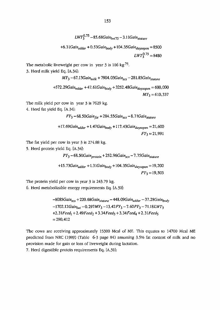
153
L W T ^ ' ^ ^ - 8 5 . - 3 . 1 ^ G a i n g , ^ , , ^ ^
+6.3lGain„(i^er +^-5'^Gaiiiijojy + l04.35Gainjaysopen =8500
LWT^-''^=mO
The metabolic liveweight per cow in year 3 is 106 kg-^^.
3. Herd milk yield Eq. [A.34]:
MXg — 67.13Gain„,jif. + 7904.03GaiHg(.g — 281. i5Gaiii^fgi„^g
+512.29Gain„jcter +41.6lGainho^y+3252A8Gaindaysopen = 600,000
A/y3 = 610,337
The milk yield per cow in year 3 is 7629 kg.
4. Herd fat yield Eq. [A.34]:
FY2-6^.50Gainfai +284.55GflHij„ -8.71Gai%a/H/-e
+17.69Gfl/H„(/^g^ + 1.47Ga//j6o^^ +117.43Ga/H^a^^ope« =21,600
^^3 =21,991
The fat yield per cow in year 3 is 274.88 kg.
5. Herd protein yield Eq. [A.34]:
PY2-6i.5QlGainproiein +252.96GaiH^„ -7.75Gfl/Hj,a/i//-e
+l5J3Gam„ctder +l-31Ga/H^o(/y + 104.35Ga/«rfa^jopen = 19,200
^73 = 19,503
The protein yield per cow in year 3 is 243.79 kg.
6. Herd metabolizable energy requirements Eq. [A.30]:
—8085Gfl//i^j.j + 220.6^GaiHgiQiiifg — 448.09Gfl//J, (/e;. — 37.28Gat/j o
-1702.12Ga/H/^,-0.291MY2-13A2FY^-7.60PY^-1U8LWT2
+2.3 lFeed\ + 2.49Feed2 + 3.34Feed2 + 3.34Feed^ +2.3 IFeed^
= 290,412
The cows are receiving approximately 15300 Meal of ME. This equates to 14700 Meal ME
predicted from NRC (1989) (Table 6-3 page 84) assuming 3.5% fat content of milk and no
provision made for gain or loss of liveweight during lactation.
7. Herd digestible protein requirements Eq. [A.31]:
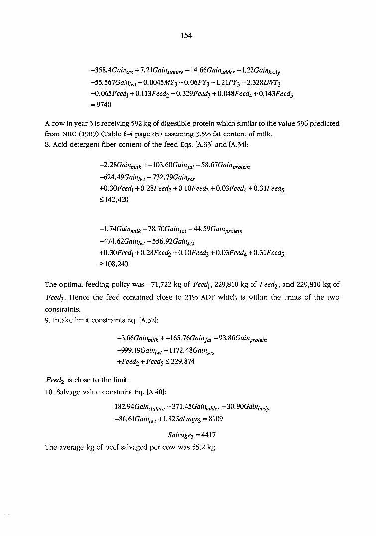
154
-358.4Gfl/\„ + 7.21Gcr//î^,a,„re -1.22Ga///èo(/^
-55.561 Gaini^t -O.OMSMFg -0.06^X3-1.2 If Xg -2.328LWT3
+0. QÇ)5Feed\ +0.113Feed2 + 0.329Feed^ + 0.048Feed4 + 0. lASFeed^
= 9740
A cow in year 3 is receiving 592 kg of digestible protein which similar to the value 596 predicted
from NRC (1989) (Table 6-4 page 85) assuming 3.5% fat content of milk.
8. Acid detergent fiber content of the feed Eqs. [A.33] and [A.34]:
-2.28Gain„,iik +-l03.60Gainfa, -5S.61Gainproiein
-624.49Ga/«/^, - 732.19Gainscs
M).3QFeed\ •¥Q.2%Feed2+0.\{iFeed2,-^Q.Q3Feedt^ + Q.3\Feed^
< 142,420
-\.lAGain„jiii^-l?,.lQGainfat protein
-474.62Gfl//j/^, -556.92Ga/Hj„
+0.30Feedi + 0.28Feed2 + 0. lOFeed:^ + 0.03Feed4 +0.3 IFeed^
>108,240
The optimal feeding policy was—71,722 kg of Feedi, 229,810 kg of Feed2, and 229,810 kg of
Feed^. Hence the feed contained close to 21% AD F which is within the limits of the two
constraints.
9. Intake limit constraints Eq. [A.32]:
-3.66Gam„,iii. +-l65J6Gamfai -93.S6Gainproiein
—999.19Gfl//j/n,j — 1 172.48GÛI//2jcs
+Feed2 +Feed^ <229,874
Feed2 is close to the limit.
10. Salvage value constraint Eq. [A.401:
182.94Gfl//ij,a,„re -371.45Gfl/H„^^e;. -30.90Ga///6o^^
-86.61Gfl/«/>^, +1.825fl/vage3 =8109
Salvage^ =4417
The average kg of beef salvaged per cow was 55.2 kg.

155
11. Calf value constraint Eq. [A.41]:
—0.047Gaingi(,ii,ff,—0.096Gaini,(]cigy — O.OOSGainijg(iy +Calf-^ =43.15
Ca//3 =43.14
Fifty-four percent of the calf crop in year 3 is sold.
12. Incidence of mastitis Eq. [A.391:
-\9A5Gainscs-Mast-i=2%.(X)
Mast-i =28.09
13. Fixed costs:
FC3 =11008
14. Variable costs for the herd Eq. [4.42]:
VC3 =51,650
15. Cashflow constraint Eq. [4.43]:
0.078^X3 +3.548^^3 -1.873^^3 -0.094Feedi
-Q.\0\Feed2 -0.134Feed3 -Q.\'i()Feed^-Q.Q95Feed^
+1.362iSfl/vflge3 — FC3 — VC3 +99.58Ca^3 — 131.3Mfl^^3
+h063Surplus2 -1.0S3deficit2 -Surplus2 + deficit'^ = 0
Surplus-^ =44,677
The net income for year 3 is $44,677.
156
References
ARC 1981. ne nutrient requirements of ruminant livestock. Commonwealth Agricultural Bureaux.
Gresham Press, Surrey UK.
Boldman, K. G., A. E. Freeman, B. L. Harris, and A. L. Kuck. 1992. Prediction of sire transmitting
abilties for linear type score. / Dairy Sci. (in press)
Dabdoub, A., and G. E. Shook. 1984. Phenotypic relationships among milk yield, somatic cell
count, and clinical mastitis. / Dairy Sci. Suppl. 1. 67:234.
Dado, A. A., D. R. Mertens, and G. E. Shook. 1990. Tlieoretical metabolizable energy and protein
requirements for milk component production. / Daity Sci. Suppl. 73:248.
Hendrichs, A. J., and G. L. Hargrove. 1987. Standards of weight and heiglit for Holstein heifers.
J. Dairy Sci. 70:653.
Lin, C. Y., A.J. McAllister, and A.J. Lee. 1985. Multitrait estimation of relationships of first lactation
yields to body weight changes in Holstein heifers. / Dairy Sci. 63:1900.
Moore R. K., B. W. Kennedy, L. R. Schaeffer, and J. E. Moxely. 1990. Relationships between
reproduction traits, age and body weight at calving in first lactation Ayrshires and Holsteins.
/ Dairy Sci. 73:835.
Moore R. K., B. W. Kennedy, L. R. Schaeffer, and J. E. Moxely. 1991. Relationships between age
and body weight and production in first lactation Ayrshires and Holsteins. /. Dairy Sci.
74:269.
Nieuwhof G. F., H. D. Norman, and F. N. Dickerson. 1989. Phenotypic trends in herd life of dairy*
cows in United States. / Dairy Sci. 72:726.
NRC 1989. Nutrient requirements of ciair)> cattle. Sixth revised Edition Update 1989. National
Academy Press, Washington, D. C., USA
Satter, L. D., and R. E. Roffler. 1975. Nitrogen requirement and utilization in dairy cattle./. Daity
Sci. 58:1219.
Schutz, M. M., L. B. Hansen., G. R. Steuernagel, and A. L. Kuck. 1990. Contributions to variation
of milk, fat, protein, and somatic cells for dairy cattle./. Dairy Sci. 73:484
Tyrrell, H. F.,andJ. T. Reid. 1965. Prediction of net energy value of cow's milk./. 48:1215.
Wiggans, G. R., and G. E. Shook. 1987. A lactation measure of somatic cell count./. Dairy Sci.
70:2666.
Welper, R. D. 1991. Estimation of variance components and response to selection for milk-
composition in Holsteins, including lactose and somatic cell score. Ph.d. Dissertation, Iowa
State Univ, Ames.

157
APPENDIX 2. LINEAR PROGRAMMING MODEL PARAMETERS
Parameters for the linear programming model are given in Tables 1 through 6.
Table 1. Geneflow parameters for milk, fat, protein yield, and liveweight and somatic
cell score
Year Milk Fat Protein Other Liveweight Somatic cell score
1 -0.975 -0.971 -0.961 -0.935 -1.142 -1.423
2 -0.068 -0.057 -0.040 0.065 -0.036 -0.223
3 0.839 0.856 0.881 1.065 1.071 0.977
4 1.746 1.770 1.801 2.065 2.178 2.176
5 2.653 2.683 2.722 3.065 3.284 3.376
6 3.560 3.597 3.643 4.065 4.390 4.576
7 4.467 4.510 4.564 5.065 5.497 5.776
8 5.375 5.424 5.485 6.065 6.603 6.975
9 6.282 6.337 6.406 7.065 7.709 8.175
10 7.189 7.251 7.327 8.065 8.816 9.375
11 8.096 8.164 8.247 9.065 9.922 10.574
12 9.003 9.078 9.168 10.065 11.029 11.774
13 9.910 9.991 10.089 11.065 12.135 12.974
14 10.817 10.905 11.010 12.065 13.242 14.174
15 11.724 11.818 11.931 13.065 14.348 15.373
16 12.631 12.732 12.852 14.065 15.455 16.573
17 13.538 13.645 13.773 15.065 16.561 17.773
18 14.445 14.559 14.693 16.065 17.667 18.972
19 15.352 15.472 15.614 17.065 18.774 20.172
20 16.259 16.385 16.535 18.065 19.880 21.372

158
Table 2. Herdlife parameters for milk, fat, protein yield, and liveweight, salvage value and
calf value
Year Milkl Fatl Protein^ Liveweight Salvage Calf value
1 -1.411E-04 -1.264E-04 -1.058E-04 -1.302E-02 5.719E-01 -4.839E-04
2 -9.837E-05 -8.708E-05 -7.173E-05 -8.811E-03 4.221E-01 -2.874E-04
3 -5.596E-05 -4.807E-05 -3.800E-05 -4.625E-03 2.724E-01 -9.384E-05
4 -1.390E-05 -9.388E-06 -4.547E-06 -5.998E-04 1.226E-01 9.348E-05
5 2.781E-05 2.897E-05 2.863E-05 3.666E-03 -2.693E-02 2.874E-04
6 6.917E-05 6.701E-05 6.152E-05 7.531E-03 -1.763E-01 4.839E-04
7 1.102E-04 1.047E-04 9.415E-05 1.166E-02 -3.265E-01 6.833E-04
8 1.509E-04 1.422E-04 1.265E-04 1.569E-02 -4.763E-01 8.812E-04
9 1.912E-04 1.793E-04 1.586E-04 1.977E-02 -6.261 E-01 1.075E-03
10 2.312E-04 2.161E-04 1.904E-04 2.387E-02 -7.759E-01 1.273E-03
11 2.709E-04 2.526E-04 2.220E-04 2.818E-02 -9.258E-01 1.469E-03
12 3.103E-04 2.888E-04 2.533E-04 3.207E-02 -1.075E+00 1.672E-03
13 3.494E-04 3.247E-04 2.844E-04 3.606E-02 -1.225E+00 1.862E-03
14 3.881 E-04 3.604E-04 3.152E-04 4.016E-02 -1.375E+00 2.056E-03
15 4.266E-04 3.957E-04 3.458E-04 4.411E-02 -1.525E+00 2.258E-03
16 4.647E-04 4.308E-04 3.761 E-04 4.827E-02 -1.675E+00 2.447E-03
17 5.025E-04 4.656E-04 4.062E-04 5.252E-02 -1.825E+00 2.639E-03
18 5.400E-04 5.001E-04 4.361 E-04 5.634E-02 -1.975E+00 2.845E-03
19 5.773E-04 5.343E-04 4.657E-04 6.054E-02 -2.125E+00 3.031 E-03
20 6.142E-04 5.683E-04 4.951 E-04 6.455E-02 -2.275E+00 3.242E-03
^Expressed as a proportion of the average per cow production in year 0.

159
Table 3. Days open parameters for milk, fat, and protein yield
Year Milkl Fatl Protein^
1 -5.313E-03 -5.307E-03 -5.318E-03
2 -5.378E-03 -5.385E-03 -5.391E-03
3 -5.421E-03 -5.436E-03 -5.435E-03
4 -5.285E-03 -5.270E-03 -5.275E-03
5 -5.354E-03 -5.365E-03 -5.366E-03
6 -5.193E-03 -5.169E-03 -5.186E-03
7 -5.249E-03 -5.239E-03 -5.245E-03
8 -5.244E-03 -5.244E-03 -5.247E-03
9 -5.330E-03 -5.335E-03 -5.337E-03
10 -5.235E-03 -5.229E-03 -5.227E-03
11 -5.339E-03 -5.331E-03 -5.334E-03
12 -5.244E-03 -5.234E-03 -5.238E-03
13 -5.384E-03 -5.401 E-03 -5.397E-03
14 -5.253E-03 -5.256E-03 -5.251E-03
15 -5.431 E-03 -5.461 E-03 -5.456E-03
16 -5.199E-03 -5.194E-03 -5.196E-03
17 -5.442E-03 -5.464E-03 -5.456E-03
18 -5.274E-03 -5.289E-03 -5.272E-03
19 -5.463E-03 -5.490E-03 -5.475E-03
20 -5.207E-03 -5.195E-03 -5.187E-03
^Expressed as a proportion of the average per cow production in year 0.

160
Table 4. Liveweight gain param
eters for salvage value
Year Liveweight
1 0.681
2 0.882
3 1.083
4 1.283
5 1.484
6 1.685
7 1.885
8 2.086
9 2.287
10 2.488
11 2.689
12 2.890
13 3.091
14
15 3.493
16 3.694
17 3.897
18 4.096
19 4.297
20 4^99
Table 5. Feed characteristics for the linear programming model
Feed Meal ME/kg feed^ kg RDP/kg feed^ kg ADF/kg feed^
1 2.31 0.06 0.30
2 2.49 0.11 0.28
3 3.34 0.33 0.10
4 3.34 0.05 0.03
5 2.31 0.14 0.31
^ME=metabolizable energy
2RDP=rumen digestible protein
^ADF=acid detergent fiber

161
APPENDIX 3. GENEFLOW FORTRAN 77 PROGRAM
Notes
This program computes the geneflow form aprogeny testing scheme where two stage
selection occurs in sires. A cycle of selection is assumed to contain the following steps:
1. Selection of young sires based on ancestry (first stage selection)
2. Progeny testing of young sires using a proportion of the population to breed
future dams
3. Selection of a group of proven sires from the progeny tested sires to breed future
dams and sires (second stage selection)
Program listing
//SI EXEC FORTVCL,FVP0PT=3
//FORT.SYSIN DD *
c gene flow simulation program B. L. HARRIS 1990
c
c function for initializing a matrix
subroutine initmat(mat,row, col,size)
integer*4 row,col,size
real*8 mat(size,size)
integer*4 i,j
do 10 i=l,row
do 10 j=l,col
mat(i,j)=0.0
10 continue
return
end
c function for initializing a vector
subroutine initvec(vect,row,size)
integer*4 row,size
real*8 vect(size)
integer*4 i
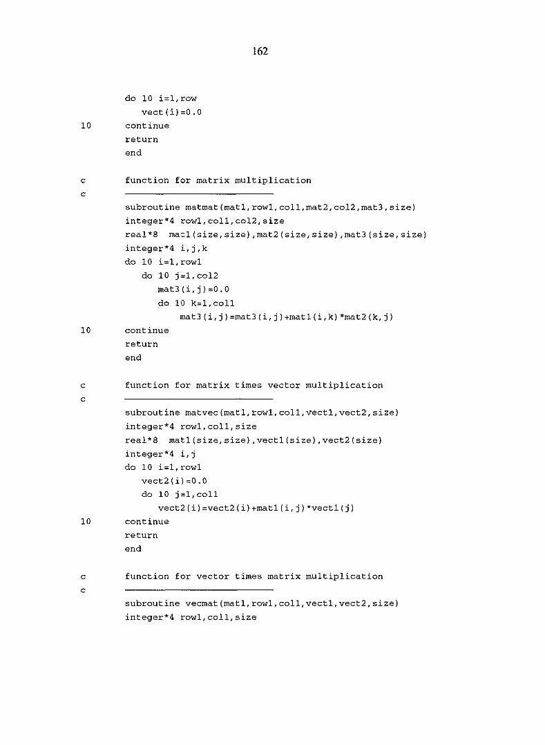
162
do 10 1=1,row
vect(i)=0.0
10 continue
return
end
c function for matrix multiplication
subroutine matmat(matl,rowl,coll,mat2,col2,mat3,size)
integer*4 rowl,coll,col2, size
real*8 matl(size,size),mat2(size,size),mat3(size,size)
integer*4 i,j,k
do 10 i=l,rowl
do 10 j=l,col2
mats(i,j)=0.0
do 10 k=l,coll
mats(i, j)=mat3(i,j)+matl(i,k)*mat2 (k, j )
10 continue
return
end
c function for matrix times vector multiplication
c
subroutine matvec(matl,rowl,coll,vect1,vect2,size)
integer*4 rowl,coll,size
real*8 matl(size,size),vectl(size),vect2(size)
integer*4 i,j
do 10 i=l,rowl
vect2(i)=0.0
do 10 j=l,coll
vect2(i)=vect2(i)+matl(i, j)*vectl(j)
10 continue
return
end
c function for vector times matrix multiplication
c
subroutine vecmat(matl,rowl,coll, vectl, vect2, size)
integer*4 rowl,coll,size

163
real*8 matl(size,size),vectl(size),vect2(size)
integer*4 i,j
do 10 i=l,coll
vect2(i)=0 .0
do 10 j=l,rowl
vect2(i)=vect2(i)+vectl(j) *matl(j , i)
10 continue
return
end
c function for vector times vector multiplication
c matrix result
c
subroutine vpv(vectl,rowl,vect2,matl, size)
integer*4 rowl,size
real*8 vectl(size),vect2(size),matl(size,size)
integer*4 i,j
do 10 i=l,rowl
do 10 j=l,rowl
matl(i,j)=vectl(i)*vect2(j)
10 continue
return
end
c function for vector times vector multiplication
c scalar result
c
subroutine vecvec(vectl,rowl,vect2,out, size)
integer*4 rowl,i,size
real*8 vectl(size),vect2(size),out
out = 0 .0
do 10 i=l,rowl
out=out+vectl(i)*vect2(i)
10 continue
return
end
c back substition routine for matrix inverse routine
c
subroutine backsub(mat,rows,index, rhs, size)

164
integer*4 rows,size, index(size)
real*8 mat(size,size),rhs(size), sum
integer*4 i,j,count,ip
count=0
do 2 0 i=l,rows
ip=index(i)
sum=rhs(ip)
rhs(ip)=rhs(i)
if(count.ne.0) then
do 10 j=count,i-l
sum=sum-mat(i,j)*rhs(j)
10 continue
else
if(sum.ne.0) then
count=i
endif
endif
rhs(i)=sum
20 continue
do 40 i=rows,l,-l
sum=rhs(i)
do 3 0 j=i+l,rows
sum= sum-mat(i,j)* rhs(j)
3 0 continue
rhs(i)=sum/mat(i,i)
40 continue
return
end
c Inverse of matrix routine uses LU decomposition and
c back substitution
c
subroutine inverse(matl,mat2,rows,type,size)
integer*4 rows,type,size
real*8 matl(size,size),mat2(size,size)
real*8 mattemp(50,50),col(50)
integer*4 i,j,index(50)
do 10 i=l,rows

165
do 10 j=l,rows
mattemp(i,j)=matl(i,j)
10 continue
call ludmp(mattemp,rows,index,type,50)
do 40 j=l,rows
do 2 0 i=l,rows
col(i)=0.0
20 continue
col(j)=1.0
call backsub(mattemp,rows, index,col,50)
do 3 0 i=l,rows
mat2(i,j)=col(i)
30 continue
40 continue
return
end
c This function performs a LU decomposition of a matrix
c
subroutine ludmp(mat,rows,index,typ,size)
integer*4 rows,size,index(size),typ
real*8 mat(size,size), tiny
real*8 big,dum,sum,temp,type
real*8 vect(50)
integer*4 i,j,k.,max
tiny=le-20
type=l.0
do 20 i=l,rows
big=0.0
do 10 j=l,rows
temp=ABS(mat(i, j) )
if(temp.gt.big) big=temp
10 continue
if(big.eg.0.0) then
typ=l
print 11
11 format(' Singular matrix encountered')
endif
vect(i)=1.0/big
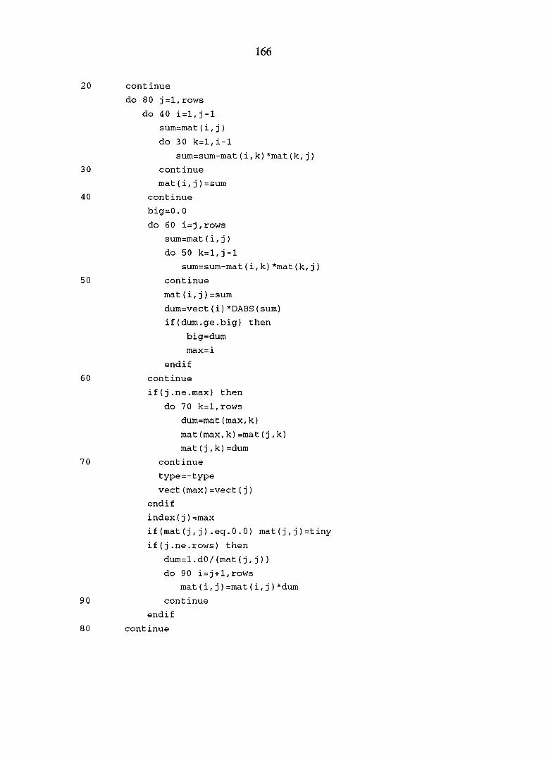
166
20 continue
do 80 j=l,rows
do 40 i=l,j-l
sum=mat{i,j)
do 30 k=l,i-1
sum=sum-mat(i,k)*mat(k,j)
30 continue
mat(i,j)=sum
40 continue
big=0.0
do 60 i=j , rows
sum=mat(i, j)
do 50 k=l,j-l
sum=sum-mat(i,k)*mat(k, j)
50 continue
mat(i,j)=sum
dum=vect(i)*DABS(sum)
if(dum.ge.big) then
big=dum
max=i
endif
60 continue
if(j.ne.max) then
do 70 k=l,rows
dum=mat(max,k)
mat(max,k)=mat(j,k)
mat(j,k)=dum
70 continue
type=-type
vect(max)=vect(j)
endif
index(j)=max
if(mat(j,j).eq.0.0) mat(j,j)=tiny
if(j.ne.rows) then
dum=l.dO/(mat(j,j))
do 90 i=j+l,rows
mat(i,j)=mat(i,j)*dum
90 continue
endif
80 continue
167
return
end
computes truncation point for a normal distribution
subroutine trunc(prop,out)
real*8 prop,out,temp
if (prop.gt.0.5) prop=prop-0.5
temp=l.0/prop
out=((DLOG(temp))**0.3633802)-0.8753044165
out=out*EXP(1.0)
out=out-(3.5*(out**2)-(out**3))*0.005
return
end
setup the phenotypic matrix for males selection index
subroutine phmale(gene,rep,pheno, aprog, prog, alact
,lact,num,phenm, size)
integer*4 size
real*8 gene(size,size),rep(size),pheno(size,size)
real*8 aprog,prog,alact,lact
real*8 phenm(size,size)
integer*4 num
integer*4 tempi,temp2,temp3
integer*4 i,j,k,l
templ=4*num
temp2=5*num
temp3=6*num
call initmat(phenm,temp2,temp2, 50)
do 40 i=l,num
do 3 0 j=l,4
do 2 0 k=l,num
do 10 1=1,4
if((l.eq.l ).and.( j.eq.l)) phenm((i-1)*4+
(k-1)*4 + 1) = (pheno(i, k) + (aprog-1)*0.25
*gene(i,k))/aprog

168
if((l.eq.l ).and.( j.eq.2)) phenm((i-l)*4+j,
(k-1)*4+1)=gene(i,k)*0.125
if((1.eg.2 ).and.( j.eq.l)) phenm{(i-l)*4 + j ,
(k-1)*4+1)=gene(i,k)*0.125
if((l.eq.2 ).and.( j.eq.2)) phenm((i-l)*4+j,
(k-1)*4+1)=(pheno(i, k)+(aprog-1)
*0.25*gene(i,k))/aprog
if((l.eq.3 ).and.(j.eq.3)) then
if(i.eq.k) phenm((i-l)*4+j,(k-l)*4+l)=
(pheno(i,k)+(lact-1)*pheno(i,k)
*rep(i))/lack
if(i.ne.k) phenm((i-l)*4+j,(k-1)*4+1)=
(pheno(i,k)+(lact-1)*gene(i,k))/lact
endif
if((l.eq.3 ).and.( j.eq.4)) phenm((i-l)*4+j,
(k-1)*4+1)=gene(i,k)*0.25
if((l.eq.4 ).and.( j.eq.3)) phenm((i-l)*4+j,
(k-1)*4+1)=gene(i,k)*0.25
if((l.eq.4 ).and.( j.eq.4)) phenm((i-l)*4+j,
(k-1)*4 + 1) = (pheno(i, k)+(aprog-1)
*0.25*gene(i,k))/aprog
10 continue
20 continue
30 continue
40 continue
do 7 0 i=l,num
do 60 j=l,4
do 50 k=l,num
if(j.eq.l) phenm((i-l)*4+j,templ+k)
=0.125*gene(i,k)
if((j.eq.2).or.(j.eq.4)) phenm((i-l)*4+j,templ+k)
* =0.25*0.25*gene(i,k)
if(j.eq.3) phenm((i-l)*4+j , templ+k)
* =0.25*gene(i,k)
phenm(templ+k,(i-l)*4+j)=phenm((i-l)*4+j,templ+k)
50 continue
60 continue
70 continue
do 90 i=l,num
do 80 j=l,num

169
phenin(templ+i, templ+j ) = (pheno (i, j ) +
* (prog-1)*0.25*gene(i,j))/prog
80 continue
90 continue
return
end
c setup the genotypic matrix for males selection index
c
subroutine genmal(gene,num,genem,size)
integer*4 num,size
real*8 gene(size,size),genem(size,size)
integer*4 tempi,temp2
integer*4 i,j,k
templ=4*num
temp2=5*num
call initmat(genem,temp2,num,50)
do 3 0 i=l,num
do 20 k=l,num
do 10 j=l,4
if(j.eq.1) genem((i-l)*4+j,k)=0.25*gene(i,k)
i f((j.eq.2).or.(j.eq.4))
* genem({i-l)*4 + j,k)=0.125*gene(i, k)
if(j.eq.3) genem((i-l)*4+j,k)=0.5*gene(i,k)
10 continue
20 continue
30 continue
do 50 i=l,num
do 40 k=l,num
genem(templ+i,k)=gene(i, k)*0.5
40 continue
50 continue
return
end
c setup female phenotypic matrix selection index
c
subroutine phfemme(gene, rep, pheno, aprog,prog,alact,lact,num.

170
phenfm,size)
integer*4 num,size
real*8 gene(size,size),rep(size),pheno(size,size)
real*8 aprog,prog,alack,lact,phenfm(size,size)
integer*4 tempi,temp2,temp3
integer*4 i,j,k,l
templ=4*num
temp2=5*num
temp3=6*num
call initmat(phenfm,temp2,temp2, 50)
do 40 i=l,num
do 30 j=l,4
do 20 k=l,num
do 10 1=1,4
if((1.eq.1).and.(j.eq.1)) phenfm((i-1)*4+],
(k-1)*4+1)=(pheno(i,k)+(aprog-1)
*0.25*gene(i,k))/aprog
if((l.eq.l).and.(j.eq.2)) phenfm((i-1)*4+j,
(k-1)*4+1)=gene(i,k)*0.125
if((l.eq.2).and.(j.eq.1)) phenfm((i-1)*4+],
(k-1)*4+1)=gene(i,k)*0.125
if((l.eq.2).and.(j.eq.2)) phenfm((i-1)*4+],
(k-1)*4+1)=(pheno(i,k)+(aprog-1)
*0.25*gene(i,k))/aprog
if((1.eq.3).and.(j.eq.3)) then
if(i.eq.k) phenfm((i-1)*4+],(k-1)*4+1)
=(pheno(i,k)+(alact-1)*pheno(i,k)
*rep(i))/alact
if(i.ne.k) phenfm((i-1)*4+j,(k-1)*4+1)
= (pheno(i, k) + (alact-1)*gene(i,k))/alact
endif
if((l.eq.3).and.(j.eq.4)) phenfm((i-1)*4+],
(k-1)*4 + 1)=gene(i, k)*0.25
if((l.eq.4).and.(j.eq.3)) phenfm((i-1)*4+],
(k-1)*4+1)=gene(i,k)*0.25
if((l.eq.4).and.(j.eq.4)) phenfm((i-1)*4+],
(k-1)*4+1)=(pheno(i,k)+(aprog-1)

171
*0.25*gene(i,k))/aprog
continue
continue
continue
continue
do 7 0 i=l,num
do 60 j=l,4
do 50 k=l,num
if(j.eq.1) phenfm((i-1)*4+j,templ+k)
=0.25*gene(i,k)
if((j.eq.2).or.(j.eq.4)) phenfm((i-1)*4+],templ+k)
=0.125*gene(i,k)
if(j.eq.3) phenfm((i-1)*4+],templ+k)
=0.5*gene(i,k)
phenfm(templ+k,(i-l)*4+j)=
phenfm((i-1)*4+j,templ+k)
continue
continue
continue
do 90 i=l,num
do 80 j=l,num
if(i.eq.j) phenfm(templ+i,templ+j)
= (pheno(i,j) + (lact-1)*pheno(i, j)*rep(i))/lact
if(i.ne.j) phenfm(templ+i,templ+j)
= (pheno(i,j) + (lact-1)*gene(i, j))/lact
continue
continue
return
end
setup the genotypic matrix for females selection index
subroutine genfmme(gene,num,genefm, size)
integer*4 size
real*8 gene(size,size),genefm(size,size)
integer*4 num
integer*4 tempi,temp2
integer*4 i,j,k
templ=4 *num
172
tenip2=5*num
call initmat(genefm,temp2, num, 50)
do 3 0 i=l,num
do 20 k=l,num
do 10 j=l,4
if(j.eq.l)
genefm((i-1)*4+j , k)=0.25*gene(i,k)
i f((j.eq.2).or.{j.eq.4))
genefm((i-l)*4+j,k)=0.125*gene(i,k)
if(j.eq.3)
genefm((i-1)*4+j , k)=0.5*gene(i,k)
continue
continue
continue
do 50 i=l,num
do 40 k=l,num
genefm{templ+i,k)=gene(i, k)
continue
continue
end
main program for multitrait gene flow simulation
Bevin Harris 1990
real*8 phentype(50,50).genetic(50,50),repeat(50)
real*8 economic(50),pmm(50),pfm(50) , pmf(50),pff(50),length
real*8 ef(50,50),em(50,50),p(50,50),q(50,50),mo(50),smo(50)
real*8 smml(50),smfl(50) , gain(4,8), sfo(50)
real*8 rmalel(50),rpmm2(50),rpmf2(50),rpfem( 50)
real*8 response(50,50),rl(50),rlf(50), r2m(50),r2f(50)
real*8 rtempl(50),rtemp2(50),rtemp3(50),qtemp(50,50)
real*8 temptwo(50,50), totresp(50, 50) , qtemp2(50,50)
real*8 phnmale(50,50),phnfem(50, 50),genmale(50,50)
real*8 invfem(50,50),invmale(50, 50) , fileout(1125,16)
real*8 intmale,intmm,intmf, intfm, prop,tnorm
real*8 aprog,progeny,femlact,lact,bfem(50)
real*8 means(8),genfem(50,50),bmale2(50)
real*8 matmale(50,50),tmale(50),wmale,bmalel(50)
real*8 temp(50, 50),tempmat(50, 50) , tempv(50)

173
real*8 genem(50,50),varbl,varb2,varbf ,phenm(50,50)
integer*4 i,j,k,1,m,type,all
integer*4 nl,n2,n3,n4,n5,n6,n7, n8
integer*4 number,male,female,stagtwo,horizon,large
integer*4 tempi,temp2,tempB
read(10,*) number
do 20 i=l,number
read(10,*)(genetic(i,j),j =1,number)
20 continue
print 11
11 format(' Genetic variance-covariance matrix read')
do 40 i=l,number
read(10,*) (phentype(i,j),j=l,number)
40 continue
print 12
12 format(' Phenotypic variance-covariance matrix read')
read(10,*) (repeat(i),i=l,number)
print 13
13 format(' Repeatibility vector read')
read(10,*) (economic(i),i=l,number)
print 14
14 format(' Economic weights vector read')
read(10,*) lact
read(10,*) femlact
readdO, *) aprog
read(10,*) progeny
read(10,*) intmale
read(10,*) intmm
read(10,*) intmf
read(10,*) intfm
read(10,*) prop
print 15
15 format(' Numbers of lactations and progeny read')
print 16
16 format(' Selection intensities and proportion selected
read(10,*) male
read(10,*) female

174
al l=inale+female
read(10,*) (pmm(i),1=1,all)
read(10,*) (pfm(i),i=l,all)
read(10,*) (pmf(i),i=l,all)
readdO,*) (pf f {i) , i = l, all)
read(10,*) stagtwo
read(10,*) horizon
large=male
call initmat(ef,all,all,50)
call initmat(em,all,all,50)
call initmat(p,all,all,50)
call initmat(g,all,all,50)
do 110 i=l,all
em(1,i)=pmm(i)+pfm(i)
ef(male+1,i)=pmf(i)+pff(i)
p(l,i)=pmm(i)+pfm(i)
p(male+1,i)=pmf(i)+pff(i)
if(i.gt.l) then
if(i.ne.male+1) then
q(i,i-l)=1.0
p(i,i-l)=1.0
endif
endif
110 continue
call initvec(mo,all,50)
call initvec(smo,all,50)
call initvec(sfo,all,50)
call initvec(smml,all,50)
call initvec(smfl,all,50)
mo(1)=1.0
sfo(male+1)=1.0
smo(1)=1.0
smml(stagtwo)=1.0
smfl(stagtwo)=1.0

175
print 17
17 format( ' Model equation vectors and matrices setup')
call trunc(prop,tnorm)
print 18
18 format(' Truncation point on normal distribution computed')
call initvec(rl, all, 50)
call initvec(rlf, all, 50)
call initvec(r2f,all,50)
call initvec(r2m,all, 50)
call initvec(rmalel,1,horizon, 50)
call initvec(rpmm2,1,horizon, 50)
call initvec(rpmf2,1,horizon, 50)
call initvec(rpfem,1,horizon, 50)
print 19
19 format(' Gene flow model starting')
do 3 00 i=l,horizon
if(i.eq.l) then
call matvec(em,all,all,smo, rtempi ,50)
call matvec(ef,all,all,smo,rtemp2,50)
do 600 j=l,all
rl(j)=rtempl(j)+rtemp2(j)
600 continue
rmalel(i)=rl(male+1)
call matvec(em,all,all,sfo,rtempi,50)
do 610 j=l,all
rlf(j)=rtempl(j)
610 continue
rpfem(i)=rlf(male+1)
end if
if(i.ne.l) then
if(male.ge.female) large=female
else large=male
if((i-1).le.large) then
if((i-1).eq.1) then
do 130 1=1,all
do 120 m=l,all
qtemp(l,m)=q(l,m)
120 continue
176
130 continue
endif
if((i-1).gt.1) then
call matmat(qtemp, ail, ail, q, ail, temptwo,50)
do 150 1=1,ail
do 140 m=l,all
qtemp(1,m)=temptwo(1,m)
140 continue
150 continue
endif
call matvec(p,ail,ail, rl, rtempl,50)
call matmat(em,ail,ail,qtemp, ail, temptwo,50)
call matvec(temptwo,ail,ail,smo,rtemp2,50)
call matmat(ef,ail,ail,qtemp,ail,temptwo,50)
call matvec(temptwo,ail, ail,smo,rtemp3,50)
do 160 j=l,all
rl(j)=rtempi(j)+rtemp2(j)+rtemp3(j)
160 continue
call matvec(p,ail,ail,rlf,rtempl,50)
call matmat(em,ail,ail,qtemp,ail, temptwo,50)
call matvec(temptwo,ail, ail, sfo,rtemp2,50)
do 170 j=l,all
rlf(j)=rtempl(j)+rtemp2(j)
17 0 continue
endif
if((i-1).gt.large) then
call matvec(p,all,all,rl, rtempl,50)
do 180 j=l,all
rl(j)=rtempl(j)
180 continue
call matvec(p,ail,ail,rlf,rtempl,50)
do 190 j=l,all
rlf(j)=rtempl(j)
19 0 continue
endif
if(i.ge.stagtwo) then
if((i-stagtwo).le.large) then
if((i-stagtwo).eq.1) then
do 210 1=1,ail
do 200 m=l,all

177
qtemp2(1,m)=q(1,m)
200 continue
210 continue
end if
if((i-stagtwo).gt.l) then
call matmat(qtemp2,all,all, q, all, temptwo,50)
do 230 1=1,all
do 220 m=l,all
qtemp2(1,m)=temptwo(1,m)
22 0 continue
230 continue
endif
call matvec(p,all,all,r2m,rtempi,50)
call matmat(em,all,all, qtemp2, all, temptwo,50)
call matvec(temptwo,all, all, smml, rtemp2,50)
do 240 j=l,all
r2m(j)=rtempl(j)+rtemp2(j)
240 continue
call matvec(p,all,all,r2f,rtempi,50)
call matmat(ef,all,all,qtemp2 ,all,temptwo,50)
call matvec(temptwo,all, all, smf1, rtemp2,50)
do 250 j=l,all
r2 f(j)=rtempi(j)+rtemp2(j)
250 continue
endif
if((i-stagtwo).eq.0) then
call matvec(em,all,all,smml,rtempl,50)
do 260 j=l,all
r2m(j)=rtempl(j)
260 continue
call matvec(ef,all,all,smfl, rtempl,50)
do 270 j=l,all
r2f(j)=rtempl(j)
27 0 continue
endif
if((i-stagtwo).gt.large) then
call matvec(p,all,all,r2m,rtempl,50)
do 280 j=l,all
r2m(j)=rtempl(j)
280 continue

178
call matvec(p,all, all,r2f, rtempl,50)
do 290 i=l,all
r2f(j)=rtempl(j)
continue
endif
endif
rmalel{i)=rl(male+1)
rpnun2 ( i) =r2m (male+1 )
rpmf2(i)=r2f(male+1)
rpfem(i)=rlf(male+1)
endif
continue
print 301
format(' Gene flow model finished')
j=5*number
call initmat(genfem,j,number, 50)
call initmat(genmale,j,number,50)
call initmat(phnmale, j , j , 50)
call initmat(phnfem,j , j , 50 )
call phmale(genetic,repeat,phentype, aprog,progeny,
femlact,lact,number,phnmale,50)
call phfemme(genetic,repeat,phentype, aprog,progeny,
femlact,lact,number,phnfem, 50)
call genmal(genetic,number,genmale,50)
call genfmme(genetic,number,genfem,50)
j =5*number
call inverse(phnfem,invfem,j,type, 50)
j =4*number
call inverse(phnmale,invmale,j , type,50)
print 21
format(' Selection parameters set')
templ=4*number
temp2=5*number
temp3=6*number

179
do 410 i=l,temp2
do 390 j=l,teinp2
phenm(i,j)=phnmale(i,j)
continue
do 400 j=l,number
genem(i,j)=genmale(i,j)
continue
continue
call matmat(invmale,tempi, tempi,genem,number,tempmat,50)
call matvec(tempmat,tempi, number,economic,bmalel,50)
call vecmat(phenm,tempi, tempi,bmalel,tempv,50)
call vecvec(tempv,tempi,bmalel,varbl,50)
wmale=(intmale*(intmale-tnorm)/varbl)
call vecmat(phenm,tempi, temp2,bmalel,tmale,50)
call vecmat(genem,tempi,number, bmalel,tempv,50)
if(varbl.gt.0.0) then
do 420 i=l,number
gain(1,i)=tempv(i)*intmale/(varbl**0.5)
continue
endif
if(varbl.le.0.0) type=l
do 430 i=temp2+l,tempB
tmale(i)=tempv(i-temp2)
continue
call vpv(tmale,temp3,tmale,matmale,50)
do 450 i=l,temp2
do 450 j=l,temp2
phenm(i,j)=phenm(i,j)-matmale(i,j)*wmale
continue
continue
do 470 i=l,temp2
do 460 j=l,number
genem(i,j)=genem(i,j)-matmale(i,j+temp2)
*wmale
continue
continue
call inverse(phenm,temp,temp2,type,50)
call matmat(temp,temp2, temp2, genem,number,tempmat,50)

180
call matvec(tempmat,temp2, number, economic,bmale2,50)
call vecmat(phenm,temp2,temp2, bmale2, tempv,50)
call vecvec(tempv,temp2,bmale2,varb2,50)
call vecmat(genem,temp2,number, bmale2, tempv,50)
if(varb2.gt.0.0) then
do 480 i=l,number
gain(2,i)=tempv(i)*intmm/(varb2**0.5)
gain{3,i)=tempv(i)*intmf/(varb2**0.5)
continue
endif
if(varb2.le.0.0) type=l
call matmat(invfem,temp2,temp2, genfem,
number,tempmat ,50)
call matvec(tempmat,temp2, number, economic, bfem,50)
call vecmat(phnfem,temp2,temp2, bfem,tempv,50)
call vecvec(tempv,temp2,bfem, varbf, 50)
call vecmat(genfem,temp2,number,bfem,tempv,50)
if(varbf.gt.0.0) then
do 490 i=l,number
gain(4,i)=tempv(i)*intfm/(varbf**0.5)
continue
endif
if(varbf.le.0.0) type=l
call initmat(totresp,number,horizon, 50)
do 530 k=l,number
do 500 i=l,horizon
response(k,i)=rmalel(i)*gain(1,k)+
rpmm2(i)*gain(2, k) +
rpmf2(i)*gain(3,k)+
rpfem(i)*gain(4,k)
continue
do 520 i=l,horizon
do 510 j=i,horizon
totresp(k,j)=totresp(k,j)+response(k,j-i+1)
continue
continue
continue

181
print 601
601 format(' Model equations finished - now printing results')
do 570 i=l,number
write{ll,797) i
write(ll,799)
do 580 j=l,horizon
write(ll,798) j,response(i,j),totresp(i,j)
580 continue
57 0 continue
798 format(i2,5x,f9.3,22x,f9.3)
797 format(' Trait2x,i3)
799 format(' year5x, 'Response',15x, ' Cumulative Response')
end
Example Input
To use this program a ASCII file containing with the following data is required:
1. Number of traits which can be less than or equal to 8
2. Genetic (co)variance matrix
3. Phenotypic (co)variance matrix
4 . Repeatibility estimates
5. Economic weights
6. Number of records the bull dam has made when the choice to bred the young
sires is made
7. Number of records the bull dam has made in her lifetime
8. Number of progeny tested daugthers the bull sires has when the choice to bred
the young sires is made
9. Number of progeny tested daugthers the sire's sire has when the choice to bred
the young sires is made
10. Number of progeny used to progeny test sires
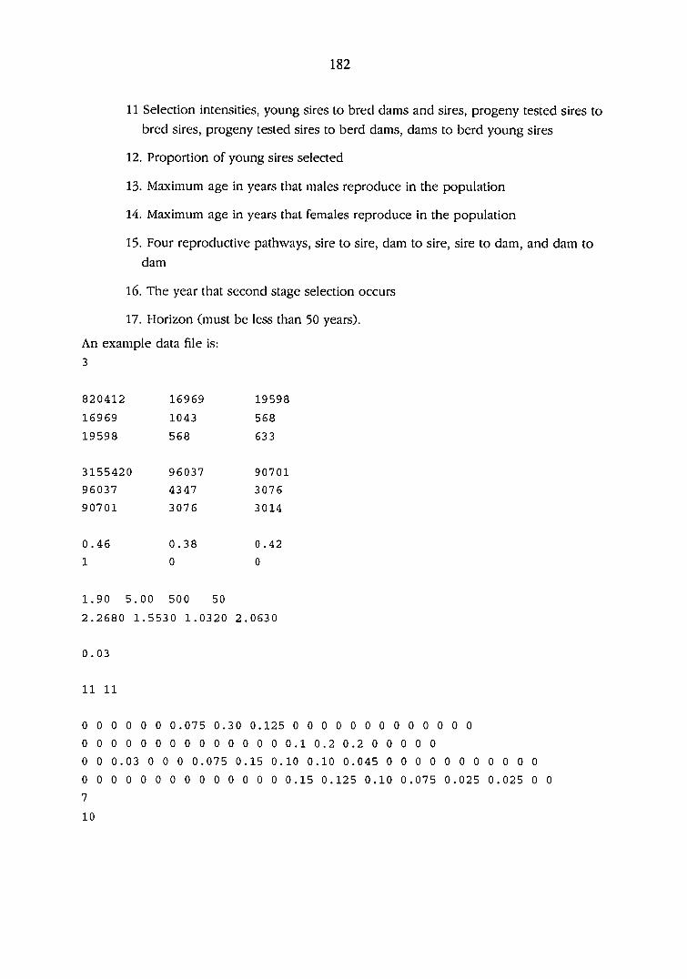
182
11 Selection intensities, young sires to bred dams and sires, progeny tested sires to
bred sires, progeny tested sires to berd dams, dams to herd young sires
12. Proportion of young sires selected
13. Maximum age in years that males reproduce in the population
14. Maximum age in years that females reproduce in the population
15. Four reproductive pathways, sire to sire, dam to sire, sire to dam, and dam to
dam
16. The year that second stage selection occurs
17. Horizon (must be less than 50 years).
An example data file is:
3
820412 16969
16969 1043
19598 568
3155420 96037
96037 4347
90701 3076
0.46 0.38
1 0
1.90 5.00 500 50
2.2680 1.5530 1.0320 2.0630
0.03
11 11
0 0 0 0 0 0 0.075 0.30 0.125 0000000000000
0 0 0 0 0 0 0 0 0 0 0 0 0 0 0 . 1 0 . 2 0 . 2 0 0 0 0 0
0 0 0.03 0 0 0 0.075 0.15 0.10 0.10 0.045 0 0 0 0 0 0 0
00000000000000 0.15 0.125 0.10 0.075 0.025
7
10
19598
568
633
90701
3076
3014
0.42
0
0 0 0 0
0.025 0 0
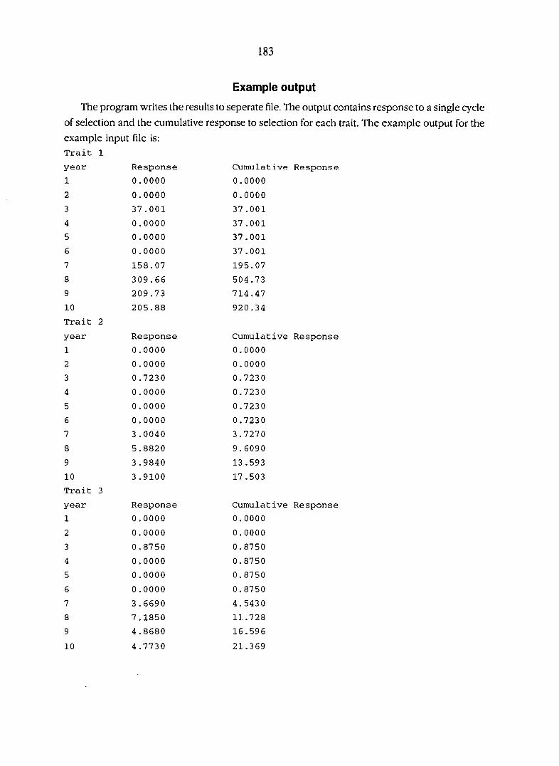
183
Example output
The program writes the results to seperate file. The output contains response to a single cycle
of selection and the cumulative response to selection for each trait. The example output for the
example input file is:
Trait 1
year Response Cumulative Response
1 0.0000 0.0000
2 0 . 0 0 0 0 0 . 0 0 0 0
3 37.001 37.001
4 0.0000 37.001
5 0.0000 37.001
6 0.0000 37.001
7 158.07 195.07
8 309.66 504.73
9 209.73 714.47
10 205.88 920.34
Trait 2
year Response Cumulative Response
1 0.0000 0.0000
2 0 . 0 0 0 0 0 . 0 0 0 0
3 0.7230 0.7230
4 0.0000 0.7230
5 0.0000 0.7230
6 0.0000 0.7230
7 3.0040 3.7270
8 5.8820 9.6090
9 3.9840 13.593
10 3.9100 17.503
Trait 3
year Response Cumulative Response
1 0 . 0 0 0 0 0 . 0 0 0 0
2 0 . 0 0 0 0 0 . 0 0 0 0
3 0.8750 0.8750
4 0.0000 0.8750
5 0.0000 0.8750
6 0.0000 0.8750
7 3.6690 4.5430
8 7.1850 11.728
9 4.8680 16.596
10 4.7730 21.369

184
APPENDIX 4. MATHEMATICA PROGRAM FOR COMPUTING LINEAR
CONSTRAINTS FROM BIVARIATE NORMAL CONTOURS
Cons t ra in t ca lcu la t ions fo r b ivar ia te normal va r iab les to account fo r
d i rec t ion and covar iance .
B . L . Har r i s 1991 . Mathemat ica Vers ion 2 .
Inpu t
1 . Input the l i s t s fo r s tandard dev ia t ions fo r the b ivar ia te normal
va r ib les (2 o r more) .
s td= {94 .78088992 ,
3 .29038982 ,
2 .75965812 ,
0 .02396177 ,
2 .23968258 ,
0 .18471568 ,
0 .27821138 ,
0 .20441265 ,
0 .23871382};
2 . Inpu t the mat r ix of cor re la t ions be tween pa i r s o f b ivar ia te normal
va r ib les .
cor r={{1 .0000 , 0 .81886 ,0 .95495 ,0 .46993 , -0 .45597 ,0 .70058 , -0 .11480 , -
0 .69319 , -0 ,04673} ,
{0 .81886 ,1 .00000 ,0 .90931 ,0 .35876 , -0 .54695 ,0 .92 579 , -0 .06526 , -
0 .43300 , -0 .13375} ,
{0 .95495 ,0 .90931 ,1 .00000 ,0 .48566 , -0 .4513 8 ,0 .86540 , -0 .06739 , -
0 .55999 , -0 .11470} ,
{0 .46993 ,0 .35876 ,0 .48566 ,1 .00000 , -0 .12691 ,0 .28276 , -0 .00064 , -
0 .16800 , -0 .05115} ,
{ - 0 . 4 5 5 9 7 , - 0 . 5 4 6 9 5 , - 0 . 4 5 1 3 8 , - 0 . 1 2 6 9 1 , 1 . 0 0 0 0 0 , -
0 .47730 ,0 .00751 ,0 .14385 ,0 .05236} ,
{0 .7 0058 ,0 .92579 ,0 .86540 ,0 .28276 , -0 .47730 ,1 .00000 , -0 .00419 , -
0 .25708 , -0 .12707} ,
{ - 0 . 1 1 4 8 0 , - 0 . 0 6 5 2 6 , - 0 . 0 6 7 3 9 , - 0 . 0 0 0 6 4 , 0 . 0 0 7 5 1 , -
0 .00419 ,1 .0000 ,0 .49211 ,0 .28956} ,
{ - 0 . 6 9 3 1 9 , - 0 . 4 3 3 0 0 , - 0 . 5 5 9 9 9 , - 0 . 1 6 8 0 0 , 0 . 1 4 3 8 5 , -
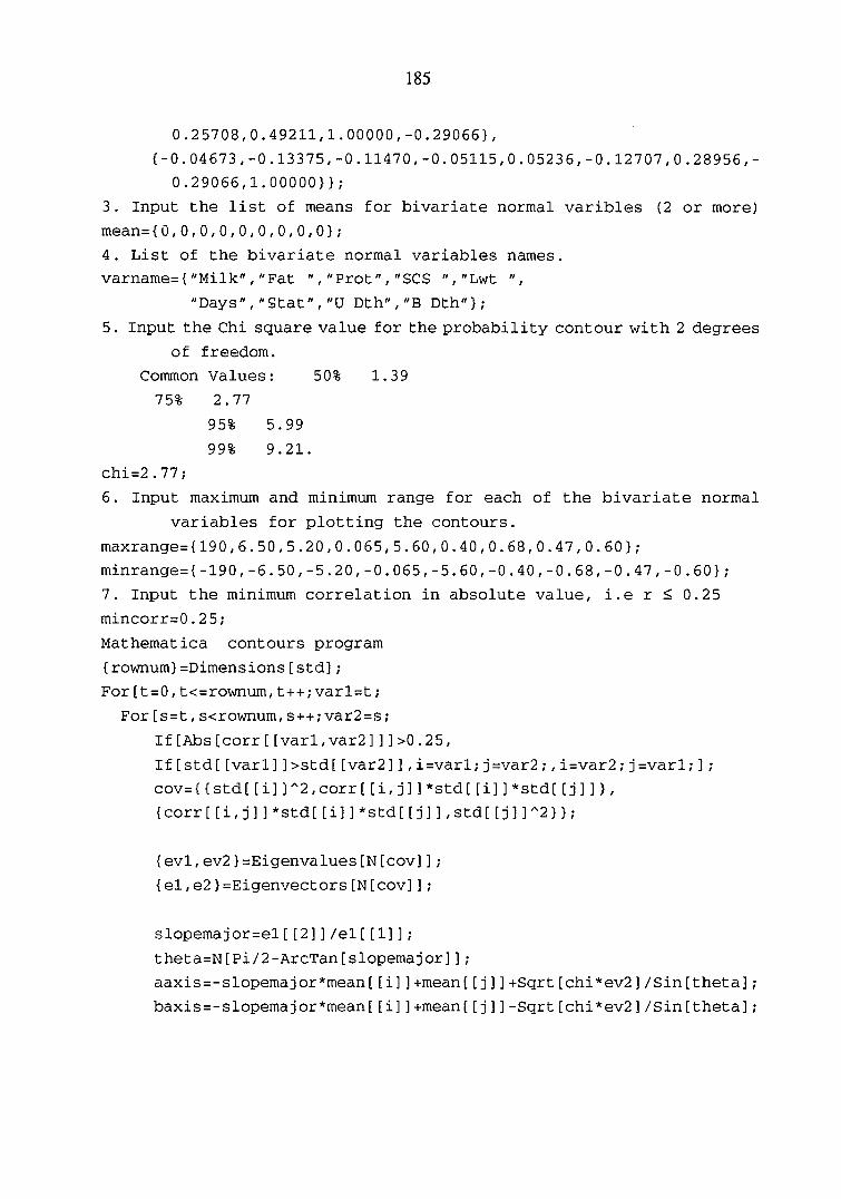
185
0 .2 5708 ,0 .49211 ,1 .00000 , -0 .29066} ,
{ -0 .04673 , -0 .13375 , -0 .11470 , -0 .05115 ,0 .0523 6 , -0 .127 07 ,0 .28956 , -
0 .29066 ,1 .00000}};
3 . Inpu t the l i s t of means fo r b ivar ia te normal va r ib les (2 o r more)
mean={0 ,0 ,0 ,0 ,0 ,0 ,0 ,0 ,0} ;
4 . L i s t o f the b ivar ia te normal va r iab les names .
va rname={"Mi lk" , "Fa t " , "Pro t" , "SCS " , "Lwt " ,
"Days" , "S ta t " , "U Dth" , "B Dth"} ;
5 . Inpu t the Chi square va lue fo r the p robab i l i ty con tour wi th 2 degrees
o f f reedom.
Common Values : 50% 1 .39
75% 2 .77
95% 5 .99
99% 9 .21 . ch i=2 .77 ;
6 . Inpu t maximum and min imum range fo r each of the b ivar ia te normal
va r iab les fo r p lo t t ing the con tours .
maxrange={190 ,6 .50 ,5 .20 ,0 .065 ,5 .60 ,0 .40 ,0 .68 ,0 .47 ,0 .60} ;
minrange={-190 , -6 .50 , -5 .20 , -0 .065 , -5 .60 , -0 .40 , -0 .68 , -0 .47 , -0 .60} ;
7 . Inpu t the min imum cor re la t ion in abso lu te va lue , i . e r < 0 .25
mincor r=0 .25 ;
Mathemat ica con tours p rogram
{rownum}=Dimens ions[s td ] ;
For [ t=0 , t<=rownum, t++;var l= t ;
For [ s= t , s<rownum,s++;var2=s ;
I f [Abs[cor r [ [var l ,va r2] ] ]>0 .25 ,
I f [ s td [ [var l ] ]>s td [ [var2] ] , i=var l ; j=var2 ; , i=var2 ; j=var l ; ] ;
cov={ {s td [ [ i ] ] ""2 , co r r [ [ i , j ] ] * s td [ [ i ] ] *s td [ [ j ] ] } ,
{cor r [ [ i , j ] ] * s td [ [ i ] ] *s td [ [ j ] ] , s td [ [ j ] ] "2}} ;
{ev l , ev2}=Eigenva lues [N[cov] ] ;
{e l , e2}^Eigenvec tors [N[cov] ] ;
s lopemajor=e l [ [2 ] ] /e l [ [1 ] ] ;
the ta=N[Pi /2 -ArcTan[s lopemajor ] ] ;
aax i s=-s lopemajor*mean[ [ i ] ]+mean[ [ j ] ]+Sqr t [ch i*ev2] /S in[ the ta ] ;
bax i s = - s lopemajor*mean[ [ i ] ]+mean[ [ j ] ] -Sqr t [ch i*ev2] /S in[ the ta ] ;
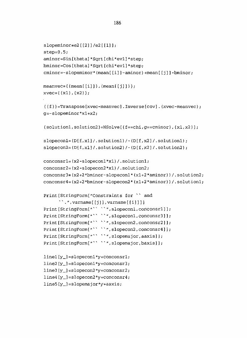
186
s lopeminor=e2[ [2] ] /e2[ [1 ] ] ;
s t ep=0 .5 ;
aminor=Sin[ thê ta ]*Sqr t [ch i*ev l ]*s tep ;
bminor=Cos[ thê ta ]*Sqr t [ch i*ev l ]*s tep ;
cminor=-s lopeminor*(mean[ [ i ] ] -aminor )+mean[ [ j ] ] -bminor ;
meanvec={{mean[ [ i ] ]} ,{mean[ [ j ] ]}} ;
xvec={{xl} ,{x2}} ;
{{f}}=Transpose[xvec-meanvec] . Inverse [cov] . (xvec-meanvec) ;
g=-s lopeminor*x l+x2;
{so lu t ion l , so lu t ion2}=NSolve[{f==chi ,g==cminor} ,{x l ,x2}] ;
s lopeconl= : (D[ f , x l ] / . so lu t ion l ) / - (D[f ,x2] / . so lu t ion l ) ;
s lopecon2=(D[f ,x l ] / . so lu t ion2) / - (D[f ,x2] / . so lu t ion2) ;
conconsr l=(x2-s lopeconl*x l ) / . so lu t ion l ;
conconsr2=(x2-s lopecon2*xl ) / . so lu t ion2 ;
conconsr3=(x2+2 *bminor -s lopeconl*(x l+2 *aminor ) ) / . so lu t ion2 ;
conconsr4=(x2+2*bminor -s lopecon2*(x l+2*aminor ) ) / . so lu t ion l ;
P r in t [S t r ingForm["Cons t ra in t s fo r and
' ' . " ,va rname[[ j ] ] ,va rname[[ i ] ] ] ]
Pr in t [S t r ingForm[" ' ' ' ' " , s lopeconl ,conconsr l ] ] ;
P r in t [S t r ingForm[" ' ' ' ^ , s lopeconl ,conconsr3] ] ;
Pr in t [S t r ingForm[" ' ' ^ , s lopecon2 ,conconsr2] ] ;
Pr in t [S t r ingForm[" ' ' ^ , s lopecon2 ,conconsr4] ] ;
P r in t [S t r ingForm[" ' " ' ^ s lopemajor ,aax i s ] J ;
Pr in t [S t r ingForm["^" ' ' " , s lopemajor ,bax is ] ] ;
l ine l [y_]=s lopeconl*y+conconsr l ;
l ine2[y_]=s lopeconl*y+conconsr3 ;
l ine ] [y_] =s lopecon2*y+conconsr2 ;
l ine4[y_]=s lopecon2*y+conconsr4 ;
l ineS[y_]=s lopemajor*y+aaxis ;

187
l ines [y_]=s lopemajor*y+baxis ;
s lopeminor=e2[ [2] ] /e2[ [1] ] ;
s t ep=N[ l /3 ] ;
aminor=Sin[ the ta ]*Sqr t [ch i*ev l ]*s tep ;
bminor=Cos[ the ta ]*Sgr t [ch i*ev l ]*s tep ;
cminor=-s lopeminor*(mean[ [ i ] ] -aminor )+mean[ [ j ] ] -bminor ;
meanvec={{mean[ [ i ] ]} ,{mean[ [ j ] ]}} ;
xvec={{xl} ,{x2}} ;
{{f}}=Transpose[xvec-meanvec] . Inverse [cov] . (xvec-meanvec) ;
g=-s lopeminor*x l+x2;
{so lu t ion l , so lu t ion2}=NSolve[{f==chi ,g==cminor} ,{x l ,x2}] ;
s lopeconl=(D[f ,x l ] / . so lu t ion l ) / - (D[f ,x2] / . so lu t ion l ) ;
s lopecon2=(D[f ,x l ] / . so lu t ion2 > / - (D[f ,x2] / . so lu t ion2) ;
conconsr l=(x2-s lopeconl*x l ) / . so lu t ion l ;
conconsr2=(x2-s lopecon2*xl ) / . so lu t ion2 ;
conconsr3=(x2+2*bminor -s lopeconl*(x l+2*aminor ) ) / . so lu t ion2 ;
conconsr4=(x2+2*bminor -s lopecon2*(x l+2*aminor ) ) / . so lu t ion l ;
P r in t [S t r ingForm["^ ^ , s lopeconl ,conconsr l ] ] ;
Pr in t [S t r ingForm[" ' " "^ , s lopeconl ,conconsrS] ] ;
Pr in t [S t r ingForm[" ' " ' ^ , s lopecon2 ,conconsr2] ] ;
P r in t [S t r ingForm[^ ^ , s lopecon2 ,conconsr4] ] ;
l ine?[y_]=s lopeconl*y+conconsr l ;
l ines [y_]=s lopeconl*y+conconsr3 ;
l ine9[y_]=s lopecon2*y+conconsr2 ;
l ine lO[y_]=s lopecon2 *y+conconsr4 ;
Graphics [P lo t [{ l ine l [ t ] , l ine2[ t ] , l ine3[ t ] , l ine4[ t ] , l ine5[ t ] , l ine6[ t ] ,
l ine?[ t ] , l ines [ t ] , l ine9[ t ] , l ine lO[ t ]} ,

188
{t,minrange[[i]],maxrange[[i ] ] },
Frame->True,RotateLabel->False,
FrameLabel->{varname [[i]],varname[[j]],
"Bivariate linear constraints",""},
PlotRange->{minrange[[j]],maxrange[[j]]}]]
]
]
Example Output
Constraints for Fat and Milk.
0 .039947 3 .63083
0 .039947 -3 .63083
0 .0169377 -3 .62845
0 .0169377 3 .62845
0 .0284386 3 .14336
0 .0284386 -3 .14336
0 .0354852 3 .3347
0 .0354852 -3 .3347
0 .0213949 -3 .33337
0 .0213949 3 .33337
Bivariate linear constraints
6
4
2
0
2
•4
6
150 -100 100 150
Milk