linear mixed models - catierepositorio.bibliotecaorton.catie.ac.cr/bitstream/... · linear mixed...
TRANSCRIPT

Linear Mixed
Models Applications in
InfoStat
Julio A. Di Rienzo
Raúl Macchiavelli
Fernando Casanoves
June, 2017

Julio A. Di Rienzo is Professor of Statistics and Biometry at
the College of Agricultural Sciences at the National
University of Córdoba, Argentina. He is director of the
InfoStat Development Team and responsible for the
implementation of the R interface presented in this
document ([email protected]).
Raúl E. Macchiavelli is Professor of Biometry at the
College of Agricultural Sciences, University of Puerto
Rico - Mayagüez ([email protected]).
Fernando Casanoves is the Head of the Biostatistics Unit, at
the Tropical Agricultural Research and Higher Education
Center (CATIE). Previously he worked at the College of
Agricultural Sciences at the National University of
Córdoba, Argentina, where he participated in the
development of InfoStat ([email protected]).
Linear mixed models : applications in InfoStat / Julio Alejandro Di Rienzo ; Raul E. Macchiavelli ;
Fernando Casanoves. - 1a edición especial - Córdoba: Julio Alejandro Di Rienzo, 2017.
Libro digital, PDF
Archivo Digital: descarga
ISBN 978-987-42-4986-9
1. Análisis Estadístico. 2. Software. 3. Aporte Educacional. I. Macchiavelli, Raul E. II. Casanoves,
Fernando III. Título CDD 519.5

AGKNOWLEDGEMENTS
The authors give thanks to the statisticians Yuri Marcela García Saavedra, Jhenny
Liliana Salgado Vásquez and Karime Montes Escobar, of the University of Tolima,
Colombia, for their critical reading of the manuscript, the reproduction of the examples
in this manual, and their contribution to some of the details of the interface.

Linear Mixed Models in InfoStat
ii
TABLE OF CONTENTS
Introduction ................................................................................................................................. 1
Requirements............................................................................................................................... 1
Extended and mixed linear models procedure ......................................................................... 1
Specification of fixed effects ....................................................................................................... 2
Specification of random effects .................................................................................................. 4
Comparison of treatment means ............................................................................................... 7
Specification of the correlation and error variance structures ............................................. 12
Specification of the correlation structure ................................................................................ 12
Specification of the fixed part ........................................................................................................... 15
Specification of the random part ...................................................................................................... 16
Specification of the error variance structure ........................................................................... 25
Analysis of a fitted model ......................................................................................................... 29
Examples of Applications of Extended and Mixed Linear Models ...................................... 33
Estimation of variance components ........................................................................................ 35
Crossed random effects with interaction ................................................................................ 57
Application of mixed models for hierarchical data ................................................................ 61
Split plots .......................................................................................................................................... 61
Split plots arranged in a RCBD ........................................................................................................ 61
Split plots in a completely randomized design .................................................................................. 72
Split-split plot ................................................................................................................................... 81
Application of mixed models for repeated measures in time ................................................. 90
Longitudinal data ............................................................................................................................. 90
Analysis of a forage establishment experiment ................................................................................. 91
Analysis of a trial for asthma drugs................................................................................................ 109
Analysis of litter decomposition bags ............................................................................................. 123
Use of mixed models to control spatial variability in agricultural experiments ................... 136
Spatial correlation .......................................................................................................................... 136
Applications of mixed models to other experimental designs .............................................. 157
Strip-plot design ............................................................................................................................. 157
Augmented design with replicated checks ...................................................................................... 178
Applications in linear regression .......................................................................................... 190
Random coefficient regression........................................................................................................ 190
Heteroscedastic regression ............................................................................................................. 194
Incomplete blocks and related designs ................................................................................. 208

Linear Mixed Models in InfoStat
iii
Alpha lattice designs ....................................................................................................................... 208
Latinized row-column design .......................................................................................................... 215
Balanced squared lattice design ..................................................................................................... 224
References ................................................................................................................................ 234
Table index .............................................................................................................................. 237
Figures index ........................................................................................................................... 237

Linear Mixed Models in InfoStat
1
Introduction
InfoStat implements a friendly interface of the R platform to estimate extended and
mixed linear models through the gls and lme procedures of the nlme library. The
reference bibliography for this implementation is Pinheiro & Bates (2004), and some of
the examples used come from this book. InfoStat communicates with R by its own
communication technology (developed by Eng. Mauricio Di Rienzo, 2016).
Requirements
To let InfoStat to have full access to R, it must be installed on your system and an
updated version of R. To perform the installation process correctly, consult the online
help in the InfoStat Help menu, submenu How to install R? and follow the instructions
given without omitting any steps.
Extended and mixed linear models
In the Statistics menu, select the Extended and mixed linear models submenu, here you
will find three options. The first option, with the heading Model estimation activates the
dialogue window for the specification of the model structure. The second option, with
the heading Model exploration, is activated when a model has been previously
estimated, and it contains a group of tools for diagnostic analysis. The third option links
to the Tutorial for mixed model analysis and estimation.

Linear Mixed Models in InfoStat
2
Specification of fixed effects
Let us begin by indicating how to adjust a fixed effects model using the Atriplex.IDB2
file located in InfoStat test datasets (File, open test data). Once this file is open, activate
the Statistics menu, the Extended and mixed linear models submenu, Model estimation
option. In the variables selection window, the dependent variables (Variables),
classification factors (Class variables) and covariates can be specified as in an analysis
of variance for fixed effects. For the data in the Atriplex.IDB2 file, Germination should
be specified as a response variable, and Size and Color as classification variables. Once
the selection is accepted, the principal window of the interface for mixed models will
appear. This window contains five tabs (Figure 1).
Figure 1: Tabs with the options for the specification of an extended and mixed linear model.
The first tab allows the user to specify the fixed effects of the model, to select options
for the presentation of results and the generation of predictions, to obtain residuals for
the model, and to specify the estimation method. The default estimation method is
restricted maximum likelihood (REML).
To the right of the window, a list containing the classification variables and covariates
declared in the variables selection window will appear. To include a factor
(classification variable) or a covariate in the fixed part of the model, the user needs only
to double click on the name of the factor o covariate that he/she wishes to include. This
action will add a line to the fixed effects list. Additional double clicks on a factor or a
covariate will successively add linear terms that are implicitly separated by a “+” sign
(additive model). By selecting the main factors and activating the “*” button, the user
may add a term that specifies an interaction between factors. For the data set in the
Atriplex.IDB2 file, include in the fixed effects model the factors Size, Color and their
interaction (Figure 2). Some of the fonts in this window have been increased in size to
improve their visualization (this is done by moving the mouse roller while pressing the
Ctrl key).
If we accept this specification, this will generate an output in the InfoStat results
window, shown below Figure 2. This is the simplest output because neither additional
model characteristics nor other analysis options have been specified. The first part

Linear Mixed Models in InfoStat
3
contains the specification of the way the estimation model was invoked in the R syntax,
and it indicates the name of the R object containing the model and its estimation, in this
case, model000_Germination_REML. This specification is of interest only to those users
who are familiar with R commands.
The second part shows measures of fit that are useful in comparing different models
fitted to a data set. AIC refers to the Akaike’s criterion, BIC to Schwarz’ Bayesian
information criterion, logLik to the logarithm of the likelihood, and Sigma to the
residual standard deviation. The third part of this output presents an analysis of variance
table and shows sequential-type hypothesis testing.
Figure 2: Window displaying the Fixed effects tab (Atriplex.IDB2 file).
Extended and mixed linear models
R specification of the model
model000_Germination_REML<-gls(Germination~1+Size+Color+Size:Color
,method="REML"
,na.action=na.omit
,data=R.data00)

Linear Mixed Models in InfoStat
4
Results for model: model000_Germination_REML
Dependent variable:Germination
Fit measurements
N AIC BIC logLik Sigma R2_0
27 160.36 169.26 -70.18 9.07 0.92 Smaller AIC and BIC is better
Sequential hypothesis testing
numDF F-value p-value
(Intercept) 1 1409.95 <0.0001
Size 2 10.49 0.0010
Color 2 90.53 <0.0001
Size:Color 4 2.29 0.0994
Specification of random effects
Random effects are associated with groups of observations. Typical examples are
repeated measurements on the same individual or the observed responses for a group of
homogeneous experimental units (blocks) or for the individuals in the same family
group, etc. These random effects are “added” to the fixed effects in a selective manner.
Because of this, in the specification of random effects it is necessary to have one or
more grouping or stratification criteria, and to choose the fixed effects to which the
associated random effects should be added. In the R lme procedure on which this
implementation is based, when more than one grouping criterion is acceptable, these are
nested or hierarchical. However, it is possible to use crossed random effects. In the
Extended and mixed linear models submenu, Random effects tab, the symbol > is used
to denote a nested factor (A>B indicates that B is nested within A); the symbol + is
used to denote crossed factors (A+B indicates that A and B are crossed factors); the
symbol * is used to denote interactions (A*B indicates the interaction between A and
B). These symbols can be written directly in the window, or, by clicking the mouse
right button on two or more previously selected factors, a window with these options
appears.
In the second tab of the model specification dialogue, we can choose the stratification or
grouping criteria and the way these incorporate random effects to fixed components. To
exemplify the specification of the random effects, let us consider the Block.IDB2 data
file. This file contains three columns: Block, Treatment and Yield. In this example, we
Linear Mixed Models in InfoStat
5
will indicate that the blocks were selected in a random manner or that they produce a
random effect (for example, if the blocks are a set of plots, their effect could be
considered random, because their response will depend on environmental conditions
that are not predictable, among other things), whereas the treatments add fixed effects.
To specify this model, the first two columns of the data file Block.IDB2 (Block and
Treatment) should be introduced as classification criteria and the last one (Yield) as a
dependent variable. The Treatment factor should be included in the Fixed effects tab as
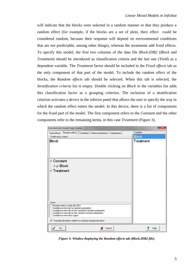
the only component of that part of the model. To include the random effect of the
blocks, the Random effects tab should be selected. When this tab is selected, the
Stratification criteria list is empty. Double clicking on Block in the variables list adds
this classification factor as a grouping criterion. The inclusion of a stratification
criterion activates a device in the inferior panel that allows the user to specify the way in
which the random effect enters the model. In this device, there is a list of components
for the fixed part of the model. The first component refers to the Constant and the other
components refer to the remaining terms, in this case Treatment (Figure 3).
Figure 3: Window displaying the Random effects tab (Block.IDB2 file).

Linear Mixed Models in InfoStat
6
The previously specified stratification criteria appear in the list of fixed terms. The
combination of both lists defines the random effects. For this, every stratification
criterion within each fixed effect is associated with a check box. When the check box is
checked, this indicates that there is a group of random effects associated with a
corresponding fixed effect. The number of random effects is equal to the number of
levels of the fixed term of the model, or equal to 1 in the case of the constant or the
covariates. The illustrated example includes a random effect induced by the blocks on
the constant.
This specification represents the following model:
; 1,.., ; 1,...,ij i j ijy b i T j B (1)
where ijy is the response to the i-th treatment in the j-th block; is the general mean
of yield; i is the fixed effects of the treatments; jb is the middle level change of
ijy
associated with the j-th block; and ij is the error term associated with observation
ijy .
T and B are the number of levels of the classification factor that correspond to the
Treatment fixed effect and to the number of blocks, respectively. The nature of these
effects is different from the fixed effects: the jb ’s are considered identically distributed
20, bN random variables whose realizations are interpreted as the effects of the
different groups or strata (blocks in this example). In these models, the jb ’s are not
estimated; instead, the 2
b parameter that characterizes its distribution is estimated. The
ij ’s are also interpreted as identically distributed 20,N random variables, and they
describe the random error associated with each observation. Moreover, the random
variables jb and
ij are assumed to be independent.
The output for this example is shown below. The new part of this output, with respect to
the example for the fixed effects linear model, is a section of parameters for the random
effects.
Extended and mixed linear models
R specification of the model
model001_Yield_REML<-lme(Yield~1+Treatment
.random=list(Block=pdIdent(~1))
.method="REML"
.na.action=na.omit
.data=R.data01
.keep.data=FALSE)

Linear Mixed Models in InfoStat
7
Results for model: model001_Yield_REML
Dependent variable:Yield
Fit measurements
N AIC BIC logLik Sigma R2_0 R2_1
20 218.77 223.73 -102.39 160.65 0.89 0.93 Smaller AIC and BIC is better
Sequential hypothesis testing
numDF denDF F-value p-value
(Intercept) 1 12 2240.00 <0.0001
Treatment 4 12 41.57 <0.0001
Random effects parameters
Covariance model for random effects: pdIdent
Formula: ~1|Block
Standard deviations relative to residual standard deviation and
correlation
(const)
(const) 0.57
In this case the estimation of b (the standard deviation of the
jb ’s relative to the
residual) is 0.57. At the beginning of the output, the estimation of , the standard
deviation of the ij ’s, is presented as 160.65. Thus, the variance of the blocks can be
calculated as: 2 2(0.57 160.65) 8385.15b
Comparison of treatment means
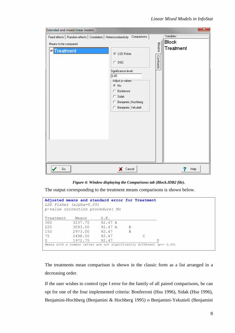
Continuing with the Comparisons tab (Figure 4), if one of the fixed terms of the model
is checked in the panel list, a means and standard errors table is obtained, as well as a
the Fisher’s LSD-type multiple comparison test (this is based on a Wald test) or a
cluster-based DGC test (Di Rienzo et al. 2002). Various corrections options for multiple
comparisons are also presented.
Linear Mixed Models in InfoStat
8
Figure 4: Window displaying the Comparisons tab (Block.IDB2 file).
The output corresponding to the treatment means comparisons is shown below.
Adjusted means and standard error for Treatment
LSD Fisher (alpha=0.05)
p-value correction procedure: No
Treatment Means S.E.
300 3237.75 92.47 A
225 3093.50 92.47 A B
150 2973.00 92.47 B
75 2498.50 92.47 C
0 1972.75 92.47 D Means with a common letter are not significantly different (p<= 0.05)
The treatments mean comparison is shown in the classic form as a list arranged in a
decreasing order.
If the user wishes to control type I error for the family of all paired comparisons, he can
opt for one of the four implemented criteria: Bonferroni (Hsu 1996), Sidak (Hsu 1996),
Benjamini-Hochberg (Benjamini & Hochberg 1995) o Benjamini-Yekutieli (Benjamini
Linear Mixed Models in InfoStat
9
& Yekutieli 2001). If the Bonferroni option is selected for this same data set, the
following result is obtained:
Adjusted means and standard error for Treatment
LSD Fisher (alpha=0.05)
p-value correction procedure: Bonferroni
Treatment Means S.E.
300 3237.75 92.47 A
225 3093.50 92.47 A B
150 2973.00 92.47 A B
75 2498.50 92.47 B
0 1972.75 92.47 B Means with a common letter are not significantly different (p<= 0.05)
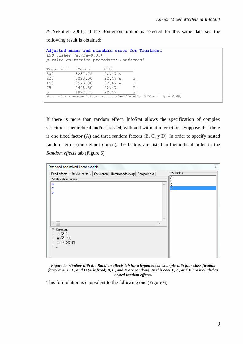
If there is more than random effect, InfoStat allows the specification of complex
structures: hierarchical and/or crossed, with and without interaction. Suppose that there
is one fixed factor (A) and three random factors (B, C, y D). In order to specify nested
random terms (the default option), the factors are listed in hierarchical order in the
Random effects tab (Figure 5)
Figure 5: Window with the Random effects tab for a hypothetical example with four classification
factors: A, B, C, and D (A is fixed; B, C, and D are random). In this case B, C, and D are included as
nested random effects.
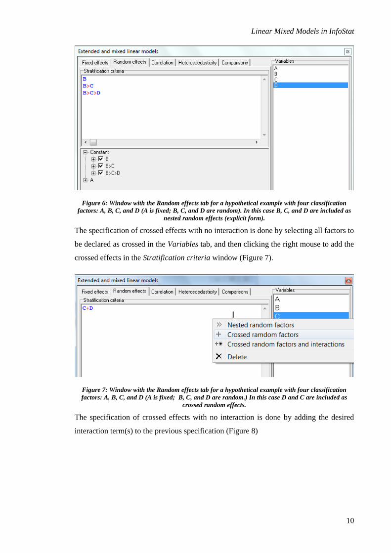
This formulation is equivalent to the following one (Figure 6)
Linear Mixed Models in InfoStat
10
Figure 6: Window with the Random effects tab for a hypothetical example with four classification
factors: A, B, C, and D (A is fixed; B, C, and D are random). In this case B, C, and D are included as
nested random effects (explicit form).
The specification of crossed effects with no interaction is done by selecting all factors to
be declared as crossed in the Variables tab, and then clicking the right mouse to add the
crossed effects in the Stratification criteria window (Figure 7).
Figure 7: Window with the Random effects tab for a hypothetical example with four classification
factors: A, B, C, and D (A is fixed; B, C, and D are random.) In this case D and C are included as
crossed random effects.
The specification of crossed effects with no interaction is done by adding the desired
interaction term(s) to the previous specification (Figure 8)

Linear Mixed Models in InfoStat
11
Figure 8: Window with the Random effects tab for a hypothetical example with four classification
factors: A, B, C, and D (A is fixed; B, C, and D are random.) In this case D and C are included as
crossed random effects with interaction.
In order to combine nested and crossed random effects, different lines can be used in the
Stratification criteria window. For example, to specify a model with C and D crossed
with interaction, and B nested in the C main effect we can write this as in Figure 9.
Figure 9: Window with the Random effects tab for a hypothetical example with four classification
factors: A, B, C, and D (A is fixed; B, C, and D are random.) In this case D and C are included as
crossed random effects with interaction, and B is nested in C.
In order to specify B and C effects nested within A (remember that A is fixed), we can
write in the Stratification criteria window as shown in Figure 10.
Figure 10: Window with the Random effects tab for a hypothetical example with four classification
factors: A, B, C, and D (A is fixed; B, C, and D are random.) In this case B and C are included as
crossed random effects, both nested within the fixed factor A.

Linear Mixed Models in InfoStat
12
In order to specify the B random effect, and the C and D crossed random effects (both
nested within B) we can write in the Stratification criteria window as shown in Figure
11.
Figure 11: Window with the Random effects tab for a hypothetical example with four classification
factors: A, B, C, and D (A is fixed; B, C, and D are random.) In this case C are D are included as
crossed random effects, both nested within the random effect B.
In all cases including non-nested random effects, the only covariance structure available
is the independence among random effects and equal variances for realizations of the
same effect. One can also specify random coefficient (regression) models, but the
sintaxis differs. See an example of random coefficient model in Applications in linear
regression.
Specification of the correlation and error variance structures
The variance and covariance structures can be modeled separately. For this, InfoStat
presents two tabs: in the Correlation tab two options are found to specify the error
correlation structure, and the Heteroscedasticity tab allows the user to select different
models for the variance function. The contents of these tabs are described below.
Specification of the correlation structure
To exemplify the use of this tool we will use an example cited in Pinheiro & Bates
(2004). The example corresponds to the “Ovary” file, which contains the data from a
study by Pierson & Ginther (1987) on the number of follicles bigger than 10 mm in
mare ovaries. These numbers were recorded through time 3 days before ovulation and
up to 3 days after the next ovulation. The data can be downloaded from the nlme library
using the menu item Applications>> Open R-data set. When this option is activated the

Linear Mixed Models in InfoStat
13
following dialogue window opens, which can differ in the number of libraries that are
installed in the user’s local R configuration (Figure 12).
Figure 12: Dialogue window for importing data from R libraries.
In this window the nlme library is checked, and to the right is the list of data files of this
library. Double clicking on “Ovary, nlme” will open an InfoStat data table containing
the corresponding data. The heading of the open table is shown below (Figure 13).

Linear Mixed Models in InfoStat
14
Figure 13: Heading of the data table (Ovary file).
A graph of the relation between the number of follicles and time is shown below (Figure
14).
Figure 14. Relationship between the number of follicles and time.
Pinheiro & Bates (2004) propose to fit a model where the number of follicles depends
linearly on sine (2*pi*Time) and cosine (2*pi*Time). This model tries to reflect the
cyclical variations of the number of follicles through the inclusion of trigonometric
functions. They also propose the inclusion of a random effect, Mare, on the constant of
the model and a first-order autocorrelation of the errors within each mare. A random
-0.25 0.00 0.25 0.50 0.75 1.00 1.25
Time
0
5
10
15
20
25
Fo
llic
les

Linear Mixed Models in InfoStat
15
effect was included to model the lack of independence that results from subject-
dependent effects expressed as parallel profiles of the number of follicles through time.
The proposed model would have the following general form:
0 1 2 02* * 2* *it i ity sin pi Time cos pi Time b (2)
where the random components are 2
0 ~ 0,i bob N and 2~ 0,it N , and are
supposed to be independent.
On the other hand, the inclusion of a first-order autocorrelation within each mare allows
the modeling of an eventual serial correlation. To specify this model in InfoStat, we will
indicate that follicles is the dependent variable, that Mare is the classification criterion,
and that Time is a covariate.
Specification of the fixed part
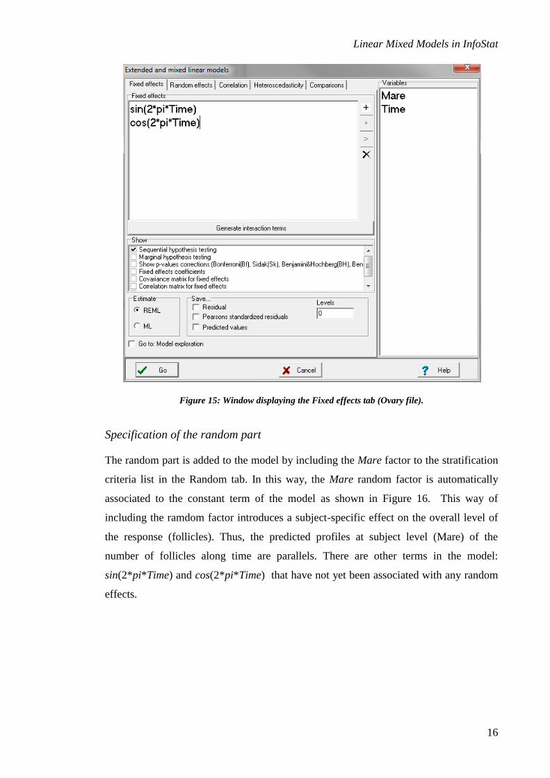
The fixed part of the model will be indicated as shown in Figure 15. InfoStat verifies
that the elements in this window correspond to the factors and covariates listed on the
right-hand side of the window.
If this is not the case, because lowercase and uppercase letters have not been used
consistently (R is sensitive to typography), then InfoStat substitutes those terms for the
appropriate ones. If there are words that InfoStat cannot interpret (such as sin, cos and
pi, in this case), then the line is marked in red when the user press <Enter>. This does
not necessarily mean that they are incorrect, but that they could be, and warns the user
to verify them.
Linear Mixed Models in InfoStat
16
Figure 15: Window displaying the Fixed effects tab (Ovary file).
Specification of the random part
The random part is added to the model by including the Mare factor to the stratification
criteria list in the Random tab. In this way, the Mare random factor is automatically
associated to the constant term of the model as shown in Figure 16. This way of
including the ramdom factor introduces a subject-specific effect on the overall level of
the response (follicles). Thus, the predicted profiles at subject level (Mare) of the
number of follicles along time are parallels. There are other terms in the model:
sin(2*pi*Time) and cos(2*pi*Time) that have not yet been associated with any random
effects.

Linear Mixed Models in InfoStat
17
Figure 16: Window displaying the Random effects tab (Ovary file).
Specification of the correlation of errors
The specification of the first-order autoregressive correlation of the errors within each
mare is indicated in the Correlation1 tab, as illustrated in Figure 17. In R, there are two
groups of correlation functions. The first corresponds to serial correlation functions,
where data are assumed to be acquired in a sequence, and the second group models
spatial correlations and the data have to be spatially referenced. In the first group we
find the following functions: compound symmetry, without structure, first-order
autoregressive, first-order continuous autoregressive, and ARMA (p,q), where p
indicates the number of autoregressive terms and q indicates the number of moving
average terms. All of these models assume that data are ordered in a sequence. By
default, InfoStat assumes the sequence in which the data are arranged in the file, but if
1 If the errors are assumed to be independent (not correlated), then the first option of the correlation
structure list should be selected (selected by default).

Linear Mixed Models in InfoStat
18
there is a variable that indexes the order of the data in a different manner, this should be
indicated in the Variable that indicates the order of observations box (to activate this
box, one of the correlation structures should be selected). This variable must be an
integer for the autoregressive option. Because of this, in the sentence translated to R
language, InfoStat adds an indication so that the variable is interpreted as an integer. In
the illustrated example, the variable Time is a real number that encodes relative time to a
reference point, and it is in an inappropriate scale to be used as an ordering criterion.
However, because the data are arranged by time within each Mare, this specification
can be omitted (Figure 17).
Figure 17: Window displaying the Correlation tab (Ovary file).
If the data are not organized in ascending order within the grouping criterion (Mare), a
variable that indicates the order must be added. To add an ordering variable to the
Variable that indicates the order of observations box, its name can be written, or
dragged with the mouse, from the variables list. It is common for the correlation
structure to be associated to a grouping criterion, Mare in this case. This is indicated in
the panel labeled Grouping variables (to activate this text box one of the correlation

Linear Mixed Models in InfoStat
19
structures must to be selected). If more than one criterion is included, InfoStat
constructs as many groups as there are combination levels in the specified classification
factors. At the bottom of the window labeled Resulting expression, the R expression that
is being specified for the component “corr=” of gls or lme is shown. This expression is
only informative and cannot be edited.
Below we present the complete output for the fitted model containing an analysis of
variance table for the fixed effects, which in this case are sequential tests on the slopes
associated with the covariates sin(2*pi*Time) and cos(2*pi*Time). Note that the
standard deviation of the random component of the constant is 0.77 times the residual
standard deviation and that the parameter phi of the autoregressive model is 0.61.
Extended and mixed linear models
R specification of the model
model006_follicles_REML<-lme(follicles~1+sin(2*pi*Time)+cos(2*pi*Time)
,random=list(Mare=pdIdent(~1))
,correlation=corAR1(form=~1|Mare)
,method="REML"
,na.action=na.omit
,data=R.data06
,keep.data=FALSE)
Results for model: model006_follicles_REML
Dependent variable:follicles
Fit measurements
N AIC BIC logLik Sigma R2_0 R2_1
308 1562.45 1584.77 -775.22 3.67 0.21 0.56 Smaller AIC and BIC is better
Sequential hypothesis testing
numDF denDF F-value p-value
(Intercept) 1 295 163.29 <0.0001
sin(2 * pi * Time) 1 295 34.39 <0.0001
cos(2 * pi * Time) 1 295 2.94 0.0877
Random effects parameters
Covariance model for random effects: pdIdent
Formula: ~1|Mare
Standard deviations relative to residual standard deviation and
correlation
(const)
(const) 0.77

Linear Mixed Models in InfoStat
20
Correlation structure
Correlation model: AR(1)
Formula: ~ 1 | Mare
Model parameters
Parameter Estim.
Phi 0.61
The predicted values by the fitted model versus time are shown in Figure 18. The black
solid line represents the estimation of the population average and corresponds to the
estimations based on the fixed part of the model. To obtain the estimates to draw this
curve, the user must indicate in the Fixed effect tab that the Predicted values are
requested. By default the Level of Predicted values is zero (indicated in the Levels edit-
box), which indicates that predictions are based only on the fixed part of the model.
The dotted curves parallel to the population average curve (solid line) are the
predictions for each mare profile derived from the inclusion of the random effect
(subject-specific) on the constant. To obtain the predictions to draw these curves the
user must indicate in the Fixed effect tab that the Predicted values of level 1 are also
requested. To do this the user must type: 0;1 in the Levels edit-box.
To check the adequacy of the model we identified the points corresponding to each
mare in Figure 14 and draw a smooth curve for each one as shown in Figure 19.
Comparing Figure 18 and Figure 19 it is clear that each mare has its own biological
timing that is over-simplified by the model we have just fitted. How do we include in
the model the subject-specific variability observed in Figure 19? The simplest way to
include this subject-specific behavior is to add more random effects to model of
equation (2). As result, we have the following model:
0 1 2
0 1 2
sin 2* * sin 2* *
sin 2* * cos 2* *
it
i i i it
y pi Time pi Time
b b pi Time b pi Time
(3)
where the random components are 2
0 ~ 0,i bob N , 2
1 1~ 0,i bb N , 2
2 2~ 0,i bb N and
2~ 0,it N
and, as a first approximation they are supposed to be mutually
independent.

Linear Mixed Models in InfoStat
21
Figure 18: Fitted functions for the population number of follicles (solid black line) and for each mare
generated by the random effect on the constant (Ovary file).
To fit model (3) we need to make some changes to the data set because of some
restrictions in the use of formulas in the Random effects tab. Therefore, we calculated
sin sin 2* *T pi Time and cos cosT = 2* pi* Time as new variables in the dataset.
In the fixed part of the model, instead of specifying a list of covariables, we specify in a
single line: sin cos1+ T + T , as shown in Figure 20. This way of specifying the fixed
part of the model does not affct the fixed effects estimations but allows us to easily
introduce the random effects: 0 1 2, ,i i ib b b . Then, in the Random effects tab, we especify
the random effecs as shown in Figure 21. Note that the covariance structure assumed for
these random has been specified as pdDiag, which means that the variances of each
random component is different and that these components are not correlated. The results
of fitting this model are shown in Figure 22.
Mare 1 Mare 2 Mare 3 Mare 4 Mare 5 Mare 6
Mare 7 Mare 8 Mare 9 Mare 10 Mare 11 Population
-0.2 -0.1 0.0 0.1 0.2 0.3 0.4 0.5 0.6 0.7 0.8 0.9 1.0 1.1 1.2
Time
2
4
6
8
10
12
14
16
18
20
PR
ED
_1
_fo
llic
les
Mare 1 Mare 2 Mare 3 Mare 4 Mare 5 Mare 6
Mare 7 Mare 8 Mare 9 Mare 10 Mare 11 Population

Linear Mixed Models in InfoStat
22
Figure 19: Smooth functions (third order polynomial) for the number of follicles (solid black lines) for
each mare generated by the random effect on the constant (Ovary file).
Figure 20: Specification of the fixed part of model (3)
-0.25 0.00 0.25 0.50 0.75 1.00 1.25
Time
0
5
10
15
20
25
Fo
llic
les

Linear Mixed Models in InfoStat
23
Figure 21: Specification of the random part of model (3). Different variances for each random effect.
Figure 22: Predicted values for the number of follicles of each mare generated by the inclusion of
random effects on all parameters of the fixed part of the model (pdDiag covariance structure)
(Ovary file).
In Figure 22 we can see the effect of adjusting subject-specific curves for each mare,
which permits more realistic representation of the mare individual profiles.
Nevertheless, from a statistical point of view, it is not appropriate to assume
independence among random effects on the parameters of a regression model. To
Mare 1 Mare 2 Mare 3 Mare 4 Mare 5 Mare 6
Mare 7 Mare 8 Mare 9 Mare 10 Mare 11
-0.2 -0.1 0.0 0.1 0.2 0.3 0.4 0.5 0.6 0.7 0.8 0.9 1.0 1.1 1.2
Time
4
6
8
10
12
14
16
18
20
22
PR
ED
_1
_fo
llic
les
Mare 1 Mare 2 Mare 3 Mare 4 Mare 5 Mare 6
Mare 7 Mare 8 Mare 9 Mare 10 Mare 11
Linear Mixed Models in InfoStat
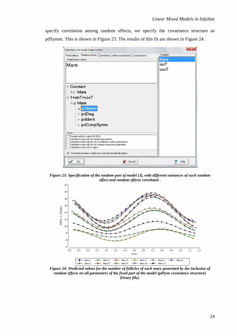
24
specify correlation among random effects, we specify the covariance structure as
pdSymm. This is shown in Figure 23. The results of this fit are shown in Figure 24.
Figure 23: Specification of the random part of model (3), with different variances of each random
effect and random effects correlated .
Figure 24: Predicted values for the number of follicles of each mare generated by the inclusion of
random effects on all parameters of the fixed part of the model (pdSym covariance structure)
(Ovary file).
Mare 1 Mare 2 Mare 3 Mare 4 Mare 5 Mare 6
Mare 7 Mare 8 Mare 9 Mare 10 Mare 11
-0.2 -0.1 0.0 0.1 0.2 0.3 0.4 0.5 0.6 0.7 0.8 0.9 1.0 1.1 1.2
Time
4
6
8
10
12
14
16
18
20
22
PR
ED
_1
_fo
llic
les
Mare 1 Mare 2 Mare 3 Mare 4 Mare 5 Mare 6
Mare 7 Mare 8 Mare 9 Mare 10 Mare 11

Linear Mixed Models in InfoStat
25
Specification of the error variance structure
This module allows the estimation of heteroscedastic models. However,
heteroscedasticity does not have a single origin and hence it can be modeled in the same
way that the correlation of errors can be modeled. The errors variance model can be
specified in the following way: 2 2var( ) ( , , )i i ig z δ where (.)g is known as the
variance function. This function can depend on the expected value ( )i of iY (the
response variable), a set of explanatory variables iz , and a parameters vector δ .
Through R, InfoStat estimates the parameters δ according to the selected variance
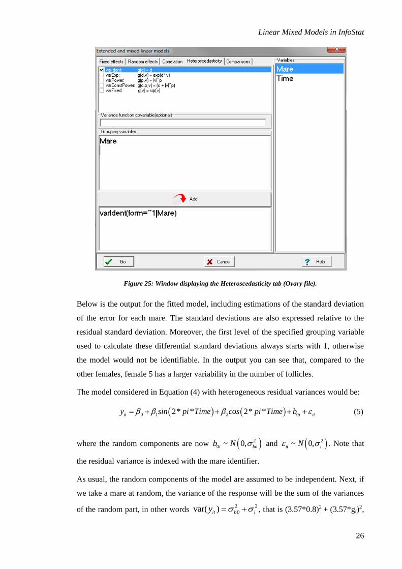
function. The Heteroscedasticity tab is shown in Figure 25. The following variance
functions are permitted: (varIdent), exponential (varExp), power (varPower), power
shifted by a constant (varConstPower), or fixed (varFixed). R allows that various
models to be overlapped, in other words, that for certain part of the dataset the variance
can be associated with one covariate, and for other part with another covariate. The
simultaneous specification of various models for the variance function is obtained by
simply marking and specifying each of the components and adding them to the variance
functions list. InfoStat constructs the appropriate sentence for R.
In the Heteroscedasticity tab for the follicles example, we have indicated that the errors
variance is different for each mare, by selecting varIdent as the variance function model
and writing Mare in Grouping variables.
Linear Mixed Models in InfoStat
26
Figure 25: Window displaying the Heteroscedasticity tab (Ovary file).
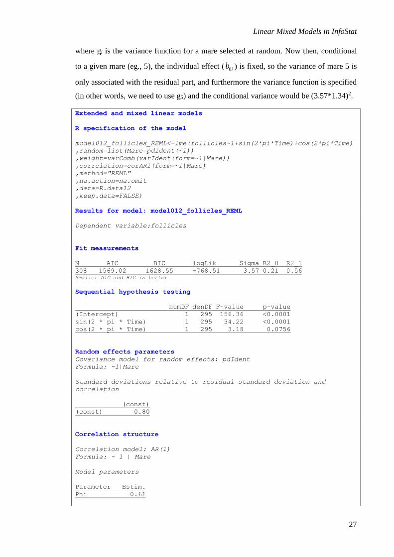
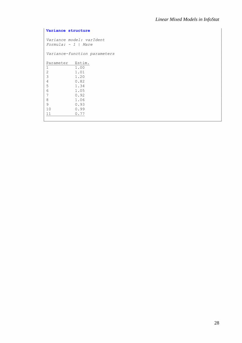
Below is the output for the fitted model, including estimations of the standard deviation
of the error for each mare. The standard deviations are also expressed relative to the
residual standard deviation. Moreover, the first level of the specified grouping variable
used to calculate these differential standard deviations always starts with 1, otherwise
the model would not be identifiable. In the output you can see that, compared to the
other females, female 5 has a larger variability in the number of follicles.
The model considered in Equation (4) with heterogeneous residual variances would be:
0 1 2 02* * 2* *it i ity sin pi Time cos pi Time b (5)
where the random components are now 2
0 ~ 0,i bob N and 2~ 0,it iN . Note that
the residual variance is indexed with the mare identifier.
As usual, the random components of the model are assumed to be independent. Next, if
we take a mare at random, the variance of the response will be the sum of the variances
of the random part, in other words 2 2
0var( )it b iy , that is (3.57*0.8)2 + (3.57*gi)2,
Linear Mixed Models in InfoStat
27
where gi is the variance function for a mare selected at random. Now then, conditional
to a given mare (eg., 5), the individual effect ( 0ib ) is fixed, so the variance of mare 5 is
only associated with the residual part, and furthermore the variance function is specified
(in other words, we need to use g5) and the conditional variance would be (3.57*1.34)2.
Extended and mixed linear models
R specification of the model
model012_follicles_REML<-lme(follicles~1+sin(2*pi*Time)+cos(2*pi*Time)
,random=list(Mare=pdIdent(~1))
,weight=varComb(varIdent(form=~1|Mare))
,correlation=corAR1(form=~1|Mare)
,method="REML"
,na.action=na.omit
,data=R.data12
,keep.data=FALSE)
Results for model: model012_follicles_REML
Dependent variable:follicles
Fit measurements
N AIC BIC logLik Sigma R2_0 R2_1
308 1569.02 1628.55 -768.51 3.57 0.21 0.56 Smaller AIC and BIC is better
Sequential hypothesis testing
numDF denDF F-value p-value
(Intercept) 1 295 156.36 <0.0001
sin(2 * pi * Time) 1 295 34.22 <0.0001
cos(2 * pi * Time) 1 295 3.18 0.0756
Random effects parameters
Covariance model for random effects: pdIdent
Formula: ~1|Mare
Standard deviations relative to residual standard deviation and
correlation
(const)
(const) 0.80
Correlation structure
Correlation model: AR(1)
Formula: ~ 1 | Mare
Model parameters
Parameter Estim.
Phi 0.61
Linear Mixed Models in InfoStat
28
Variance structure
Variance model: varIdent
Formula: ~ 1 | Mare
Variance-function parameters
Parameter Estim.
1 1.00
2 1.01
3 1.20
4 0.82
5 1.34
6 1.05
7 0.92
8 1.06
9 0.93
10 0.99
11 0.77

Linear Mixed Models in InfoStat
29
Analysis of a fitted model
When InfoStat fits an extended or mixed linear model with the Estimation menu, the
Analysis-exploration of the estimated models menu is activated. In this dialogue, various
tabs are shown, as seen in Figure 26.
Figure 26: Model exploration window displaying the Diagnostic tab (Atriplex.IDB2 file).
The example used in this case is from the Atriplex.IDB2 file, with which two fixed
effects models where estimated: model000_PG_REML, which contains the effects Size,
Color and their interaction, and model001_PG_REML, which only contains the main
effects Size and Color.
The Models tab only appears in the case that there is more than one estimated model and
shows a list of the evaluated models in a check-list. The selected models are listed along
with their respective summary statistics and a hypothesis test of model equality; the
applicability of the latter should be interpreted with caution, since not all of the models
are strictly comparable. In any case, the AIC and BIC criteria are good indicators for
the selection of a more parsimonious model.

Linear Mixed Models in InfoStat
30
The purpose of the Linear combinations tab is to test linear combinations hypotheses.
The null hypothesis is that the expected value of the linear combination is zero. This
dialogue window lists the fixed parameters of the model that were selected from the list
shown on the right-hand side of the screen (Important: the last one on the list is always
selected by default). At the bottom of the screen, there is an edition field where the
constants of the linear combination can be specified. As the coefficients are added, the
corresponding parameters are colored to facilitate the specification of the constants, as
shown in Figure 27.
Figure 27: Model exploration window displaying the Linear combination tab (Atriplex.IDB2 file).
Finally, the Diagnostic tab has three subtabs (Figure 26). The first, identified as
“Residuals vs…” has devices to easy generate boxplot graphs for the standardized
residuals vs. each of the fixed factors of the model, or scatter plots of the standardized
residuals and the covariates of the model, and scatter plots of the standardized residuals
vs. the fitted values. In the same way, it is possible to obtain the normal Q-Q plot. The
second tab, identified as “ACF-SV”, allows the user to generate a graph of the

Linear Mixed Models in InfoStat
31
autocorrelation function (useful for the diagnosis of serial correlations), and the third
one, identified as LevelPlot, allows the user to generate residuals vs. spatial correlations
graphs to construct a map of the directions and intensity of the residuals. This tool is
useful in spatial correlation diagnostics.
To exemplify the use of the ACF-FV tab, let us consider the follicles example (Ovary
file). In this example it is argued that the purpose of including the first-order
autoregressive term was to correct a lack of independence generated by the
discrepancies between the individual cycles of every mare with respect to the individual
cycles that only differed from the average population by a constant. The serial
autocorrelation graph of the residuals that corresponds to a model without the inclusion
of the first-order autocorrelation shows a clear autoregressive pattern (Figure 28). On
the other hand, the residual autocorrelation graph for the model that includes the
autocorrelation through a first-order autoregressive term corrects the lack of
independence (Figure 29).
Figure 28: Residual autocorrelation function of the model shown in Equation, excluding serial
autocorrelation.

Linear Mixed Models in InfoStat
32
Figure 29: Residual autocorrelation function of the model presented in Equation (2), including serial
autocorrelation.
The devices on the Diagnostic tab allow the researcher to quickly diagnose any eventual
problem with the fit of the fixed part as well as for the random part of the model. The
next section provides examples illustrating the use of these tools more extensively.

Linear Mixed Models in InfoStat
33
Examples of Applications of Extended and Mixed Linear Models


Estimation of variance components
In research areas such as animal or plant breeding, the estimation of the variance
components it is of particular interest. These are used to obtain heritability, response to
the selection, additive genetic variance, genetic differentiation coefficients, etc. The
mixed linear models can be used to estimate the variance components using restricted
maximum likelihood (REML) estimators.
In many genetic studies, several populations are used which are represented by one or
more individuals of different families. In this case we have two factors in the model: the
populations and the families within each population. To exemplify the use of variance
components, the data file VarCom.IDB2 (Navarro et al. 2005) is used. These data come
from a trial with seven cedar populations (Cedrela odorata L.) with a total of 115
families. Some families have repetitions available while others do not. Moreover, the
number of families within each population is not the same. The registered variables are
average seed length (length), stem diameter (diameter), stem length, and number of
leaves in cedar seedlings.
In addition to estimating the variance components, the researchers are also interested in
comparing the population means. We can study various inference spaces, according to
the design and the interests of the researchers. If the populations are a random sample of
a large set of populations, then the inference will be aimed at this large set of
populations. The effect of the studied populations is random, and the interest will be the
estimation of the variance components due to the variance among populations and
among the families within the populations. Another point of interest will be the BLUP
predictors of the random effects (especially those of the population effects).
If the inference is oriented only toward the studied populations, the population effect is
fixed, and the main interest is to estimate and compare the population means. If the
population mean is interpreted as an average throughout all possible families of that
particular population (not only those studied), then the family effect is random. In this
case, it would be of interest to estimate the variance component due to variance among
families within the populations, and to predict the effects of the studied families
(BLUP).

Linear Mixed Models in InfoStat
36
A third inference space is when the interest resides only in the studied populations and
families. In this case both effects are fixed. This kind of model has several limitations,
both in its interpretation and in its implementation. Due to this, we do not study this
model in this tutorial.
For the analysis of the VarCom.IDB2 data file, the first two discussed cases will be
fitted:
Model 1: Random populations and random families
Model 2: Fixed populations and random families
First, we select the Statistics menu; then the Extended and mixed linear models
submenu, and then Model estimation. When the selection is done, the variables selection
window will show, where we specify Length, Diameter, Stem length and number of
leaves as dependent variables, and Population and Family as classification variables
(Figure 30).
Figure 30: Variables selection window for extended and mixed linear models (VarCom.IDB2 file).
Model 1: For the estimation of the variance components, the variables should be
specified as in Figure 30. Afterwards, in the Random effects tab, indicate first
Population and then Family, since R assumes that the different random components that
Linear Mixed Models in InfoStat
37
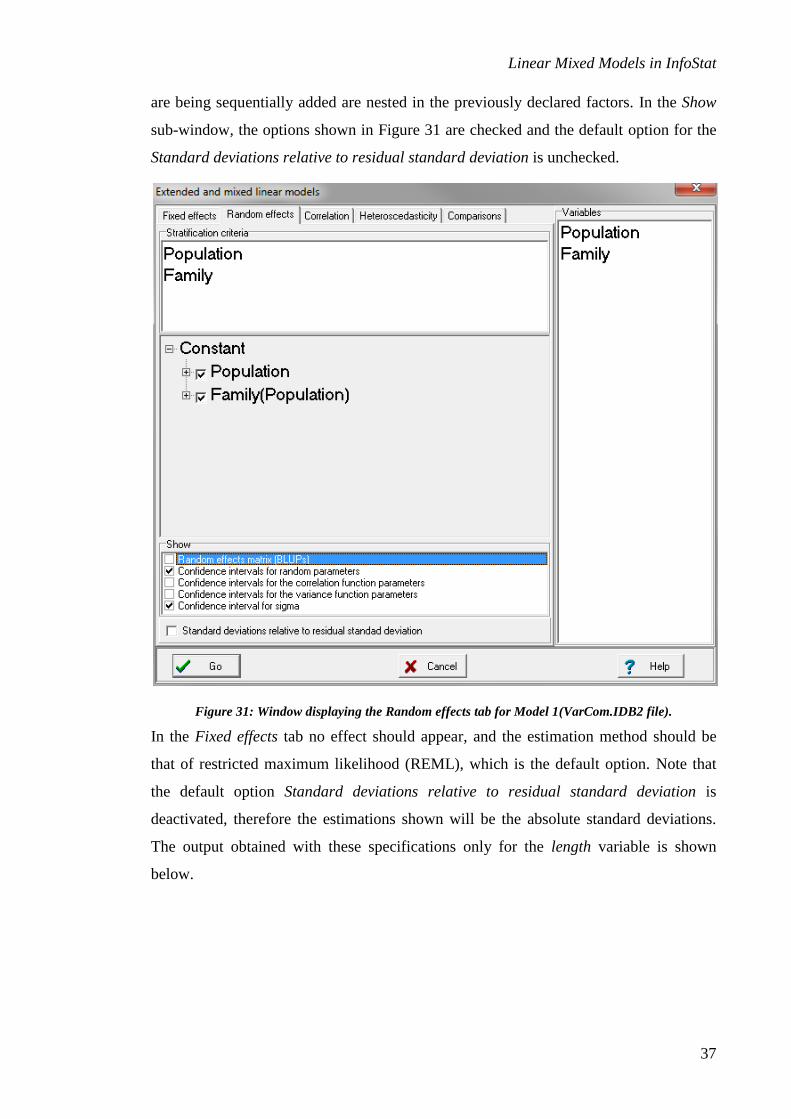
are being sequentially added are nested in the previously declared factors. In the Show
sub-window, the options shown in Figure 31 are checked and the default option for the
Standard deviations relative to residual standard deviation is unchecked.
Figure 31: Window displaying the Random effects tab for Model 1(VarCom.IDB2 file).
In the Fixed effects tab no effect should appear, and the estimation method should be
that of restricted maximum likelihood (REML), which is the default option. Note that
the default option Standard deviations relative to residual standard deviation is
deactivated, therefore the estimations shown will be the absolute standard deviations.
The output obtained with these specifications only for the length variable is shown
below.

Linear Mixed Models in InfoStat
38
Extended and mixed linear models
R specification of the model
model006_length_REML<-lme(length~1
,random=list(Population=pdIdent(~1)
,Family=pdIdent(~1))
,method="REML"
,na.action=na.omit
,data=R.data06
,keep.data=FALSE)
Results for model: model006_length_REML
Dependent variable:length
Fit measurements
N AIC BIC logLik Sigma R2_0 R2_1 R2_2
214 2016.47 2029.91 -1004.23 21.53 0.51 0.76 Smaller AIC and BIC is better
Sequential hypothesis testing
numDF denDF F-value p-value
(Intercept) 1 108 22.68 <0.0001
Random effects parameters
Covariance model for random effects: pdIdent
Formula: ~1|Population
Standard deviations and correlations
(const)
(const) 27.16
Covariance model for random effects: pdIdent
Formula: ~1|Family in Population
Standard deviations and correlations
(const)
(const) 14.80
Confidece intervals (95%) for the random effects parameters
Formula: ~1|Population
LB(95%) Est. UB(95%)
sd(const) 15.09 27.16 48.89
Formula: ~1|Family in Population
LB(95%) Est. UB(95%)
sd(const) 10.72 14.80 20.43
Confidece interval (95%) for sigma
lower est. upper
sigma 18.77 21.53 24.70
Linear Mixed Models in InfoStat
39
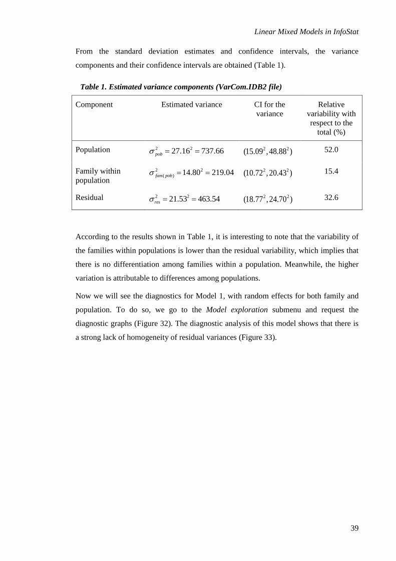
From the standard deviation estimates and confidence intervals, the variance
components and their confidence intervals are obtained (Table 1).
Table 1. Estimated variance components (VarCom.IDB2 file)
Component Estimated variance CI for the
variance
Relative
variability with
respect to the
total (%)
Population 2 227.16 737.66pob 2 2(15.09 ,48.88 ) 52.0
Family within
population
2 2
( ) 14.80 219.04fam pob 2 2(10.72 ,20.43 ) 15.4
Residual 2 221.53 463.54res 2 2(18.77 ,24.70 ) 32.6
According to the results shown in Table 1, it is interesting to note that the variability of
the families within populations is lower than the residual variability, which implies that
there is no differentiation among families within a population. Meanwhile, the higher
variation is attributable to differences among populations.
Now we will see the diagnostics for Model 1, with random effects for both family and
population. To do so, we go to the Model exploration submenu and request the
diagnostic graphs (Figure 32). The diagnostic analysis of this model shows that there is
a strong lack of homogeneity of residual variances (Figure 33).

Linear Mixed Models in InfoStat
40
Figure 32: Model exploration window displaying the Diagnostic tab for Model 1 (VarCom.IDB2 file).
Figure 33: Diagnostic graphs obtained for the variable Length, Model 1 (VarCom.IDB2 file).
In Figure 33, the standardized Pearson residuals are approximations of the errors, and
because of this, the heteroscedasticity observed should be modeled at this level.
Linear Mixed Models in InfoStat
41
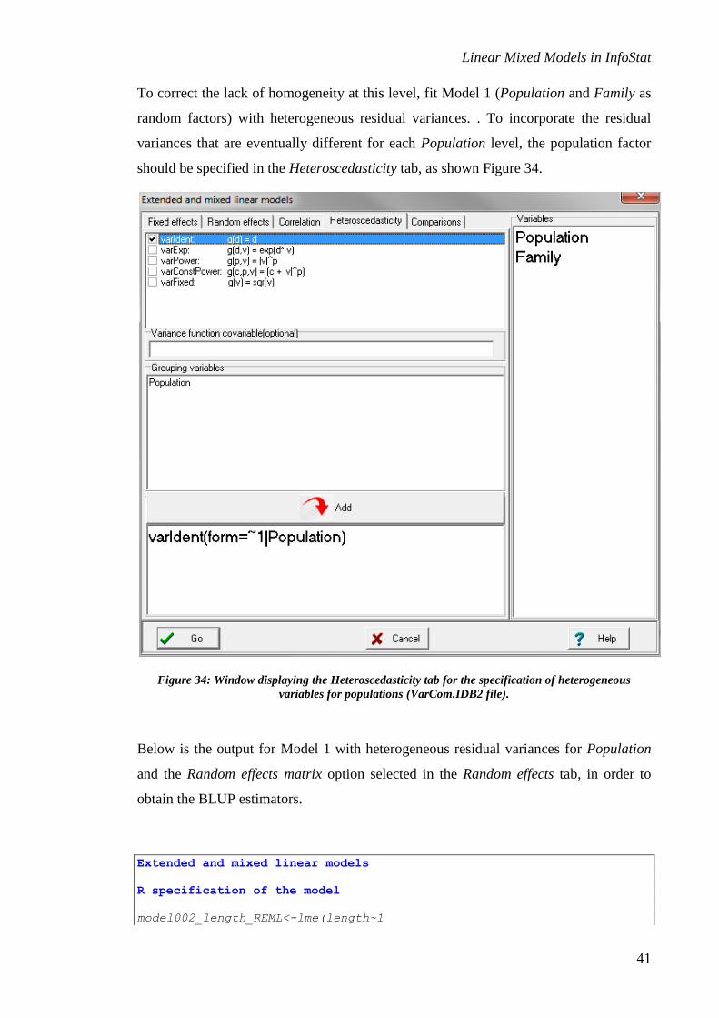
To correct the lack of homogeneity at this level, fit Model 1 (Population and Family as
random factors) with heterogeneous residual variances. . To incorporate the residual
variances that are eventually different for each Population level, the population factor
should be specified in the Heteroscedasticity tab, as shown Figure 34.
Figure 34: Window displaying the Heteroscedasticity tab for the specification of heterogeneous
variables for populations (VarCom.IDB2 file).
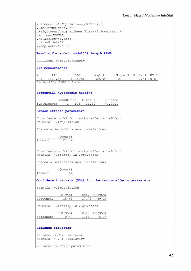
Below is the output for Model 1 with heterogeneous residual variances for Population
and the Random effects matrix option selected in the Random effects tab, in order to
obtain the BLUP estimators.
Extended and mixed linear models
R specification of the model
model002_length_REML<-lme(length~1
Linear Mixed Models in InfoStat
42
,random=list(Population=pdIdent(~1)
,Family=pdIdent(~1))
,weight=varComb(varIdent(form=~1|Population))
,method="REML"
,na.action=na.omit
,data=R.data02
,keep.data=FALSE)
Results for model: model002_length_REML
Dependent variable:length
Fit measurements
N AIC BIC logLik Sigma R2_0 R2_1 R2_2
214 1872.14 1905.75 -926.07 2.32 0.51 0.51 Smaller AIC and BIC is better
Sequential hypothesis testing
numDF denDF F-value p-value
(Intercept) 1 108 21.59 <0.0001
Random effects parameters
Covariance model for random effects: pdIdent
Formula: ~1|Population
Standard deviations and correlations
(const)
(const) 27.72
Covariance model for random effects: pdIdent
Formula: ~1|Family in Population
Standard deviations and correlations
(const)
(const) 1.56
Confidece intervals (95%) for the random effects parameters
Formula: ~1|Population
LB(95%) Est. UB(95%)
sd(const) 15.61 27.72 49.24
Formula: ~1|Family in Population
LB(95%) Est. UB(95%)
sd(const) 0.47 1.56 5.14
Variance structure
Variance model: varIdent
Formula: ~ 1 | Population
Variance-function parameters

Linear Mixed Models in InfoStat
43
Parameter Estim.
Charagre 1.00
Escarcega 13.09
Esclavos 11.64
La Paz 15.94
Pacífico Sur 2.81
Xpujil 13.38
Yucatán 12.54
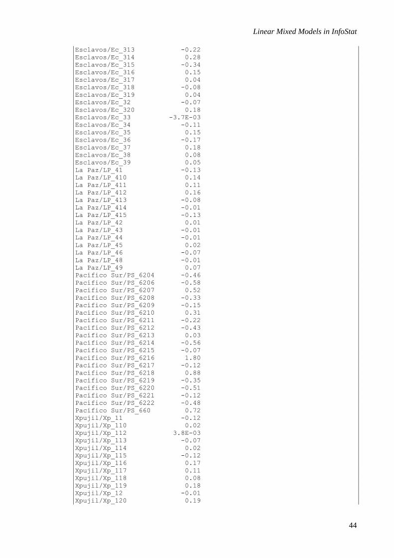
Random effects coefficients (BLUP) (~1|Population)
const
Charagre -41.20
Escarcega 15.42
Esclavos 16.12
La Paz 19.80
Pacífico Sur -36.51
Xpujil 23.29
Yucatán 3.08
Random effects coefficients (BLUP) (~1|Family in Population)
const
Charagre/Ch_71 -1.07
Charagre/Ch_710 0.59
Charagre/Ch_711 1.31
Charagre/Ch_712 1.42
Charagre/Ch_713 -0.95
Charagre/Ch_714 -1.07
Charagre/Ch_715 -0.70
Charagre/Ch_72 0.70
Charagre/Ch_73 -0.83
Charagre/Ch_74 -0.35
Charagre/Ch_75 -0.59
Charagre/Ch_76 -0.08
Charagre/Ch_77 -0.47
Charagre/Ch_78 0.48
Charagre/Ch_79 1.48
Escarcega/Es_1126 7.2E-04
Escarcega/Es_1127 0.18
Escarcega/Es_1128 0.14
Escarcega/Es_1129 0.07
Escarcega/Es_1130 3.6E-04
Escarcega/Es_1131 -0.06
Escarcega/Es_1132 0.21
Escarcega/Es_1133 0.01
Escarcega/Es_1134 -0.11
Escarcega/Es_1135 -0.09
Escarcega/Es_1136 -0.08
Escarcega/Es_1137 -0.17
Escarcega/Es_1138 0.16
Escarcega/Es_1139 -0.08
Escarcega/Es_1142 0.08
Escarcega/Es_1148 -0.20
Esclavos/Ec_31 -0.08
Esclavos/Ec_310 0.08
Esclavos/Ec_311 -0.07
Esclavos/Ec_312 -0.03
Linear Mixed Models in InfoStat
44
Esclavos/Ec_313 -0.22
Esclavos/Ec_314 0.28
Esclavos/Ec_315 -0.34
Esclavos/Ec_316 0.15
Esclavos/Ec_317 0.04
Esclavos/Ec_318 -0.08
Esclavos/Ec_319 0.04
Esclavos/Ec_32 -0.07
Esclavos/Ec_320 0.18
Esclavos/Ec_33 -3.7E-03
Esclavos/Ec_34 -0.11
Esclavos/Ec_35 0.15
Esclavos/Ec_36 -0.17
Esclavos/Ec_37 0.18
Esclavos/Ec_38 0.08
Esclavos/Ec_39 0.05
La Paz/LP_41 -0.13
La Paz/LP_410 0.14
La Paz/LP_411 0.11
La Paz/LP_412 0.16
La Paz/LP_413 -0.08
La Paz/LP_414 -0.01
La Paz/LP_415 -0.13
La Paz/LP_42 0.01
La Paz/LP_43 -0.01
La Paz/LP_44 -0.01
La Paz/LP_45 0.02
La Paz/LP_46 -0.07
La Paz/LP_48 -0.01
La Paz/LP_49 0.07
Pacífico Sur/PS_6204 -0.46
Pacífico Sur/PS_6206 -0.58
Pacífico Sur/PS_6207 0.52
Pacífico Sur/PS_6208 -0.33
Pacífico Sur/PS_6209 -0.15
Pacífico Sur/PS_6210 0.31
Pacífico Sur/PS_6211 -0.22
Pacífico Sur/PS_6212 -0.43
Pacífico Sur/PS_6213 0.03
Pacífico Sur/PS_6214 -0.56
Pacífico Sur/PS_6215 -0.07
Pacífico Sur/PS_6216 1.80
Pacífico Sur/PS_6217 -0.12
Pacífico Sur/PS_6218 0.88
Pacífico Sur/PS_6219 -0.35
Pacífico Sur/PS_6220 -0.51
Pacífico Sur/PS_6221 -0.12
Pacífico Sur/PS_6222 -0.48
Pacífico Sur/PS_660 0.72
Xpujil/Xp_11 -0.12
Xpujil/Xp_110 0.02
Xpujil/Xp_112 3.8E-03
Xpujil/Xp_113 -0.07
Xpujil/Xp_114 0.02
Xpujil/Xp_115 -0.12
Xpujil/Xp_116 0.17
Xpujil/Xp_117 0.11
Xpujil/Xp_118 0.08
Xpujil/Xp_119 0.18
Xpujil/Xp_12 -0.01
Xpujil/Xp_120 0.19

Linear Mixed Models in InfoStat
45
Xpujil/Xp_122 -0.21
Xpujil/Xp_123 -0.27
Xpujil/Xp_15 0.02
Xpujil/Xp_16 0.03
Xpujil/Xp_17 0.03
Xpujil/Xp_18 -0.05
Xpujil/Xp_19 0.07
Yucatán/Yu_1111 -0.17
Yucatán/Yu_1114 -0.19
Yucatán/Yu_1115 -0.04
Yucatán/Yu_1116 0.02
Yucatán/Yu_1117 0.05
Yucatán/Yu_1118 0.03
Yucatán/Yu_1119 0.10
Yucatán/Yu_1121 -0.06
Yucatán/Yu_1122 0.20
Yucatán/Yu_1123 -0.09
Yucatán/Yu_1124 -0.05
Yucatán/Yu_1125 0.20
Confidence interval (95%) for sigma
lower est. upper
sigma 1.59 2.32 3.38
This model shows lower AIC and BIC values than the model without heterogeneous
variances for Population and Family within Population. Note that the population
variances are very different: the La Paz population has the highest estimated variance,
(15.94*2.32)2 = 1367.57, while the population with the lowest variance has a variance
of (1*2.32)2 = 5.38. When we compare the models with heterogeneous and
homogeneous variances by means of a likelihood ratio test, we confirm that the model
with heterogeneous variances is best (p<0.0001), as shown in the following output.
Comparison of models
Call Model df AIC BIC logLik Test L.Ratio p-value
Model000_Long_REML 1 1 4 2016.47 2029.91 -1004.23
Model001_Long_REML 2 2 10 1872.14 1905.75 -926.07 1 vs 2 156.33 <0.0001
The residuals obtained for Model 1 with different residual variances in each population
do not show heteroscedasticity problems, and they show an improvement in the
distributional assumptions (Q-Q plot) with respect to Model 1 with homogeneous
variances (Figure 35).

Linear Mixed Models in InfoStat
46
Figure 35: Diagnostic graphs obtained for the variable Length, Model 1 with heterogeneous residual
variables for populations (VarCom.IDB2 file).
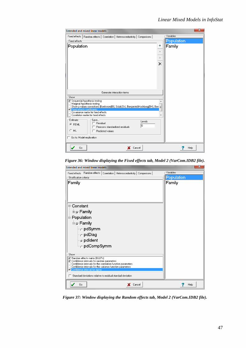
Model 2: For this model, Population should be declared in the Fixed effects tab. Note
that Fixed effects coefficients has also been selected in this tab (Figure 36). In the
Random effects tab, Family has been declared as random, the default option of Family
as an effect on the Constant (intercept) has been deselected, and Family as affecting the
parameters of the Population effect has been selected. The covariance matrix of random
effects assigned to populations is assumed independent (pdIdent). The Random effects
matrix (BLUP’s), Confidence intervals for random parameters and Confidence interval
for sigma options (Figure 37) have also been selected. In the Comparisons tab the DGC
option is selected for Population (Figure 38).
Linear Mixed Models in InfoStat
47
Figure 36: Window displaying the Fixed effects tab, Model 2 (VarCom.IDB2 file).
Figure 37: Window displaying the Random effects tab, Model 2 (VarCom.IDB2 file).

Linear Mixed Models in InfoStat
48
Figure 38: Window displaying the Comparisons tab, Model 2 (VarCom.IDB2 file)..
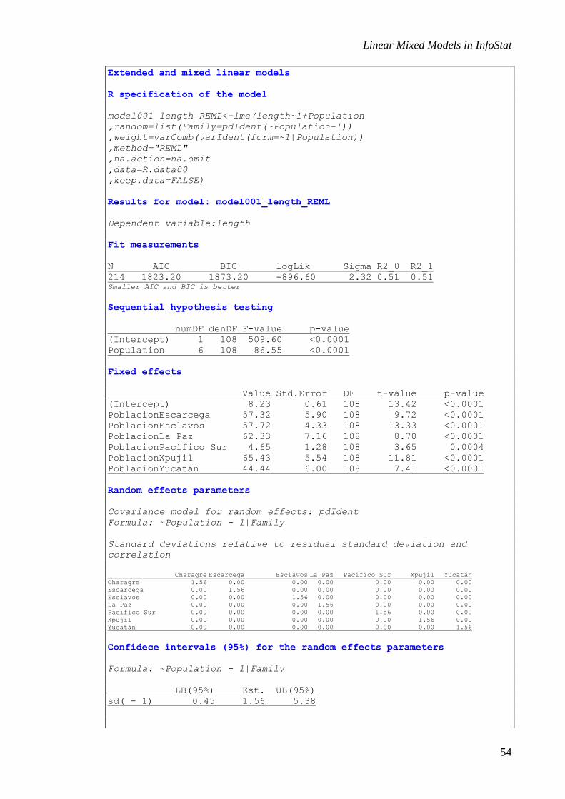
The output corresponding to these specifications is shown below:
Extended and mixed linear models
R specification of the model
model001_length_REML<-lme(length~1+Population
,random=list(Family=pdIdent(~Population-1))
,method="REML"
,na.action=na.omit
,data=R.data00
,keep.data=FALSE)
Results for model: model001_length_REML
Dependent variable:length
Fit measurements
N AIC BIC logLik Sigma R2_0 R2_1
214 1967.65 1997.64 -974.82 21.54 0.51 0.75 Smaller AIC and BIC is better
Sequential hypothesis testing
numDF denDF F-value p-value
(Intercept) 1 108 601.79 <0.0001
Population 6 108 27.23 <0.0001

Linear Mixed Models in InfoStat
49
Fixed effects
Value Std.Error DF t-value p-value
(Intercept) 8.23 5.75 108 1.43 0.1551
PopulationEscarcega 56.89 8.03 108 7.08 <0.0001
PopulationEsclavos 57.72 7.46 108 7.74 <0.0001
PopulationLa Paz 62.24 8.13 108 7.66 <0.0001
PopulationPacífico Sur 4.65 7.53 108 0.62 0.5382
PopulationXpujil 65.45 7.72 108 8.48 <0.0001
PopulationYucatán 44.44 8.40 108 5.29 <0.0001
Random effects parameters
Covariance model for random effects: pdIdent
Formula: ~Population - 1|Family
Standard deviations and correlations
Charagre Escarcega Esclavos La Paz Pacífico Sur XpujilYucatán
Charagre 14.79 0.00 0.00 0.00 0.00 0.00 0.00
Escarcega 0.00 14.79 0.00 0.00 0.00 0.00 0.00
Esclavos 0.00 0.00 14.79 0.00 0.00 0.00 0.00
La Paz 0.00 0.00 0.00 14.79 0.00 0.00 0.00
Pacífico Sur 0.00 0.00 0.00 0.00 14.79 0.00 0.00
Xpujil 0.00 0.00 0.00 0.00 0.00 14.79 0.00
Yucatán 0.00 0.00 0.00 0.00 0.00 0.00 14.79
Confidece intervals (95%) for the random effects parameters
Formula: ~Population - 1|Family
LB(95%) Est. UB(95%)
sd( - 1) 10.71 14.79 20.42
Random effects coefficients (BLUP) (~Population - 1|Family)
LI(95%) est. LS(95%)
sd( - 1) 10.71 14.79 20.42
Random effects coefficients (BLUP) (~Population - 1|Family)
Charagre Escarcega Esclavos La Paz Pacífico Sur Xpujil Yucatán
Ch_71 -1.08 0.00 0.00 0.00 0.00 0.00 0.00
Ch_710 0.62 0.00 0.00 0.00 0.00 0.00 0.00
Ch_711 1.34 0.00 0.00 0.00 0.00 0.00 0.00
Ch_712 1.47 0.00 0.00 0.00 0.00 0.00 0.00
Ch_713 -0.96 0.00 0.00 0.00 0.00 0.00 0.00
Ch_714 -1.08 0.00 0.00 0.00 0.00 0.00 0.00
Ch_715 -0.71 0.00 0.00 0.00 0.00 0.00 0.00
Ch_72 0.73 0.00 0.00 0.00 0.00 0.00 0.00
Ch_73 -0.84 0.00 0.00 0.00 0.00 0.00 0.00
Ch_74 -0.35 0.00 0.00 0.00 0.00 0.00 0.00
Ch_75 -0.60 0.00 0.00 0.00 0.00 0.00 0.00
Ch_76 -0.07 0.00 0.00 0.00 0.00 0.00 0.00
Ch_77 -0.48 0.00 0.00 0.00 0.00 0.00 0.00
Ch_78 0.50 0.00 0.00 0.00 0.00 0.00 0.00
Ch_79 1.53 0.00 0.00 0.00 0.00 0.00 0.00
Ec_31 0.00 0.00 -6.04 0.00 0.00 0.00 0.00
Ec_310 0.00 0.00 5.36 0.00 0.00 0.00 0.00
Ec_311 0.00 0.00 -5.56 0.00 0.00 0.00 0.00
Ec_312 0.00 0.00 -2.65 0.00 0.00 0.00 0.00
Ec_313 0.00 0.00 -16.00 0.00 0.00 0.00 0.00
Ec_314 0.00 0.00 20.66 0.00 0.00 0.00 0.00
Ec_315 0.00 0.00 -25.46 0.00 0.00 0.00 0.00
Ec_316 0.00 0.00 10.95 0.00 0.00 0.00 0.00
Ec_317 0.00 0.00 2.69 0.00 0.00 0.00 0.00
Ec_318 0.00 0.00 -5.80 0.00 0.00 0.00 0.00
Ec_319 0.00 0.00 2.94 0.00 0.00 0.00 0.00
Ec_32 0.00 0.00 -5.56 0.00 0.00 0.00 0.00
Ec_320 0.00 0.00 12.89 0.00 0.00 0.00 0.00

Linear Mixed Models in InfoStat
50
Ec_33 0.00 0.00 -0.46 0.00 0.00 0.00 0.00
Ec_34 0.00 0.00 -7.99 0.00 0.00 0.00 0.00
Ec_35 0.00 0.00 10.95 0.00 0.00 0.00 0.00
Ec_36 0.00 0.00 -12.84 0.00 0.00 0.00 0.00
Ec_37 0.00 0.00 12.89 0.00 0.00 0.00 0.00
Ec_38 0.00 0.00 5.36 0.00 0.00 0.00 0.00
Ec_39 0.00 0.00 3.67 0.00 0.00 0.00 0.00
Es_1126 0.00 -0.06 0.00 0.00 0.00 0.00 0.00
Es_1127 0.00 16.20 0.00 0.00 0.00 0.00 0.00
Es_1128 0.00 16.63 0.00 0.00 0.00 0.00 0.00
Es_1129 0.00 6.49 0.00 0.00 0.00 0.00 0.00
Es_1130 0.00 -0.04 0.00 0.00 0.00 0.00 0.00
Es_1131 0.00 -7.09 0.00 0.00 0.00 0.00 0.00
Es_1132 0.00 19.12 0.00 0.00 0.00 0.00 0.00
Es_1133 0.00 1.15 0.00 0.00 0.00 0.00 0.00
Es_1134 0.00 -10.25 0.00 0.00 0.00 0.00 0.00
Es_1135 0.00 -10.94 0.00 0.00 0.00 0.00 0.00
Es_1136 0.00 -7.58 0.00 0.00 0.00 0.00 0.00
Es_1137 0.00 -16.32 0.00 0.00 0.00 0.00 0.00
Es_1138 0.00 14.26 0.00 0.00 0.00 0.00 0.00
Es_1139 0.00 -10.30 0.00 0.00 0.00 0.00 0.00
Es_1142 0.00 7.71 0.00 0.00 0.00 0.00 0.00
Es_1148 0.00 -18.99 0.00 0.00 0.00 0.00 0.00
LP_41 0.00 0.00 0.00 -18.43 0.00 0.00 0.00
LP_410 0.00 0.00 0.00 18.95 0.00 0.00 0.00
LP_411 0.00 0.00 0.00 14.82 0.00 0.00 0.00
LP_412 0.00 0.00 0.00 20.89 0.00 0.00 0.00
LP_413 0.00 0.00 0.00 -12.12 0.00 0.00 0.00
LP_414 0.00 0.00 0.00 -2.41 0.00 0.00 0.00
LP_415 0.00 0.00 0.00 -18.67 0.00 0.00 0.00
LP_42 0.00 0.00 0.00 1.23 0.00 0.00 0.00
LP_43 0.00 0.00 0.00 -1.93 0.00 0.00 0.00
LP_44 0.00 0.00 0.00 -1.68 0.00 0.00 0.00
LP_45 0.00 0.00 0.00 1.96 0.00 0.00 0.00
LP_46 0.00 0.00 0.00 -9.69 0.00 0.00 0.00
LP_48 0.00 0.00 0.00 -2.39 0.00 0.00 0.00
LP_49 0.00 0.00 0.00 9.48 0.00 0.00 0.00
PS_6204 0.00 0.00 0.00 0.00 -2.13 0.00 0.00
PS_6206 0.00 0.00 0.00 0.00 -2.73 0.00 0.00
PS_6207 0.00 0.00 0.00 0.00 2.48 0.00 0.00
PS_6208 0.00 0.00 0.00 0.00 -1.52 0.00 0.00
PS_6209 0.00 0.00 0.00 0.00 -0.67 0.00 0.00
PS_6210 0.00 0.00 0.00 0.00 1.51 0.00 0.00
PS_6211 0.00 0.00 0.00 0.00 -1.03 0.00 0.00
PS_6212 0.00 0.00 0.00 0.00 -2.01 0.00 0.00
PS_6213 0.00 0.00 0.00 0.00 0.18 0.00 0.00
PS_6214 0.00 0.00 0.00 0.00 -2.61 0.00 0.00
PS_6215 0.00 0.00 0.00 0.00 -0.31 0.00 0.00
PS_6216 0.00 0.00 0.00 0.00 8.55 0.00 0.00
PS_6217 0.00 0.00 0.00 0.00 -0.55 0.00 0.00
PS_6218 0.00 0.00 0.00 0.00 4.18 0.00 0.00
PS_6219 0.00 0.00 0.00 0.00 -1.64 0.00 0.00
PS_6220 0.00 0.00 0.00 0.00 -2.37 0.00 0.00
PS_6221 0.00 0.00 0.00 0.00 -0.55 0.00 0.00
PS_6222 0.00 0.00 0.00 0.00 -2.25 0.00 0.00
PS_660 0.00 0.00 0.00 0.00 3.46 0.00 0.00
Xp_11 0.00 0.00 0.00 0.00 0.00 -14.96 0.00
Xp_110 0.00 0.00 0.00 0.00 0.00 2.35 0.00
Xp_112 0.00 0.00 0.00 0.00 0.00 -0.09 0.00
Xp_113 0.00 0.00 0.00 0.00 0.00 -7.12 0.00
Xp_114 0.00 0.00 0.00 0.00 0.00 1.61 0.00
Xp_115 0.00 0.00 0.00 0.00 0.00 -12.46 0.00
Xp_116 0.00 0.00 0.00 0.00 0.00 15.93 0.00
Xp_117 0.00 0.00 0.00 0.00 0.00 10.11 0.00
Xp_118 0.00 0.00 0.00 0.00 0.00 6.95 0.00
Xp_119 0.00 0.00 0.00 0.00 0.00 16.91 0.00
Xp_12 0.00 0.00 0.00 0.00 0.00 -2.14 0.00
Xp_120 0.00 0.00 0.00 0.00 0.00 18.36 0.00
Xp_122 0.00 0.00 0.00 0.00 0.00 -20.72 0.00
Xp_123 0.00 0.00 0.00 0.00 0.00 -27.03 0.00
Xp_15 0.00 0.00 0.00 0.00 0.00 1.86 0.00
Xp_16 0.00 0.00 0.00 0.00 0.00 2.99 0.00
Xp_17 0.00 0.00 0.00 0.00 0.00 3.95 0.00
Xp_18 0.00 0.00 0.00 0.00 0.00 -4.94 0.00
Xp_19 0.00 0.00 0.00 0.00 0.00 8.44 0.00
Yu_1111 0.00 0.00 0.00 0.00 0.00 0.00 -14.89

Linear Mixed Models in InfoStat
51
Yu_1114 0.00 0.00 0.00 0.00 0.00 0.00 -16.59
Yu_1115 0.00 0.00 0.00 0.00 0.00 0.00 -3.24
Yu_1116 0.00 0.00 0.00 0.00 0.00 0.00 1.86
Yu_1117 0.00 0.00 0.00 0.00 0.00 0.00 4.53
Yu_1118 0.00 0.00 0.00 0.00 0.00 0.00 2.83
Yu_1119 0.00 0.00 0.00 0.00 0.00 0.00 8.66
Yu_1121 0.00 0.00 0.00 0.00 0.00 0.00 -5.18
Yu_1122 0.00 0.00 0.00 0.00 0.00 0.00 17.15
Yu_1123 0.00 0.00 0.00 0.00 0.00 0.00 -7.85
Yu_1124 0.00 0.00 0.00 0.00 0.00 0.00 -4.45
Yu_1125 0.00 0.00 0.00 0.00 0.00 0.00 17.15
Confidece interval (95%) for sigma
lower est. upper
sigma 18.77 21.54 24.71
Adjusted means and standard error for Population
DGC (alpha=0.05)
Population Means S.E.
Xpujil 73.68 5.16 A
La Paz 70.47 5.74 A
Esclavos 65.95 4.75 A
Escarcega 65.12 5.61 A
Yucatán 52.67 6.13 A
Pacífico Sur 12.88 4.87 B
Charagre 8.23 5.75 B Means with a common letter are not significantly different (p<= 0.05)
The following example is an estimation of the BLUP for some families of the
population Charagre:
,71 71( )
,72 72( )
,73 73( )
,74 74( )
ˆˆ ˆˆ 8.2296 0 ( 1.0823) 7.1473
ˆˆ ˆˆ 8.2296 0 0.7277 8.9573
ˆˆ ˆˆ 8.2296 0 ( 0.8396) 7.3900
ˆˆ ˆˆ 8.2296 0 ( 0.354
cha cha cha
cha cha cha
cha cha cha
cha cha cha
Y
Y
Y
Y
2) 7.8754
The BLUP for family 42 of La Paz population is:
,42 42( )ˆˆ ˆˆ 8.2296 62.2374 1.2297 71.6967lpaz lpaz lpazY
Now we will conduct the fitness analysis for Model 2. In the Model exploration
submenu the diagnostic graphs are requested (Figure 39).

Linear Mixed Models in InfoStat
52
Figure 39: Model exploration window displaying the Diagnostic tab, Model 2 (VarCom.IDB2 file).
The Pearson’s standardized conditional residuals vs. fitted values graph (Figure 40)
shows heterogeneous residual variances for the Length variable.

Linear Mixed Models in InfoStat
53
Figure 40: Diagnostic graphs obtained for the variable Length, Model 2 (VarCom.IDB2 file).
With respect to the distributional assumptions, it is important to emphasize that, when
heteroscedasticity exists, the Q-Q plot should not be interpreted until this problem is
solved. To incorporate heterogeneous variables of the Population effect, the Population
factor should be specified in the Heterogeneity tab, as shown in Figure 34.
This model has lower AIC and BIC values than does the model without heterogeneous
variances for Population. Note that the variances of the populations are very different:
The population La Paz has a highest estimated variance, (15.94*2.32)2 = 1367.57, while
the lowest variance, for Charagre, is (1*2.32)2 = 5.38.
Linear Mixed Models in InfoStat
54
Extended and mixed linear models
R specification of the model
model001_length_REML<-lme(length~1+Population
,random=list(Family=pdIdent(~Population-1))
,weight=varComb(varIdent(form=~1|Population))
,method="REML"
,na.action=na.omit
,data=R.data00
,keep.data=FALSE)
Results for model: model001_length_REML
Dependent variable:length
Fit measurements
N AIC BIC logLik Sigma R2_0 R2_1
214 1823.20 1873.20 -896.60 2.32 0.51 0.51 Smaller AIC and BIC is better
Sequential hypothesis testing
numDF denDF F-value p-value
(Intercept) 1 108 509.60 <0.0001
Population 6 108 86.55 <0.0001
Fixed effects
Value Std.Error DF t-value p-value
(Intercept) 8.23 0.61 108 13.42 <0.0001
PoblacionEscarcega 57.32 5.90 108 9.72 <0.0001
PoblacionEsclavos 57.72 4.33 108 13.33 <0.0001
PoblacionLa Paz 62.33 7.16 108 8.70 <0.0001
PoblacionPacífico Sur 4.65 1.28 108 3.65 0.0004
PoblacionXpujil 65.43 5.54 108 11.81 <0.0001
PoblacionYucatán 44.44 6.00 108 7.41 <0.0001
Random effects parameters
Covariance model for random effects: pdIdent
Formula: ~Population - 1|Family
Standard deviations relative to residual standard deviation and
correlation
Charagre Escarcega Esclavos La Paz Pacífico Sur Xpujil Yucatán
Charagre 1.56 0.00 0.00 0.00 0.00 0.00 0.00
Escarcega 0.00 1.56 0.00 0.00 0.00 0.00 0.00
Esclavos 0.00 0.00 1.56 0.00 0.00 0.00 0.00
La Paz 0.00 0.00 0.00 1.56 0.00 0.00 0.00
Pacífico Sur 0.00 0.00 0.00 0.00 1.56 0.00 0.00
Xpujil 0.00 0.00 0.00 0.00 0.00 1.56 0.00
Yucatán 0.00 0.00 0.00 0.00 0.00 0.00 1.56
Confidece intervals (95%) for the random effects parameters
Formula: ~Population - 1|Family
LB(95%) Est. UB(95%)
sd( - 1) 0.45 1.56 5.38

Linear Mixed Models in InfoStat
55
Variance structure
Variance model: varIdent
Formula: ~ 1 | Population
Variance-function parameters
Parameter Estim.
Charagre 1.00
Esclavos 11.64
Escarcega 13.09
La Paz 15.94
Pacífico Sur 2.81
Xpujil 13.38
Yucatán 12.55
To prove that this less parsimonious model is the one with the better fit, we conducted a
likelihood ratio test, and the output is shown below.
Comparison of models
Model df AIC BIC logLik Test L.Ratio p-value
001 9 1967.65 1997.64 -974.82
002 15 1823.20 1873.20 -896.60 1 vs 2 156.44 <0.0001
The model with heterogeneous variances for the different populations is better than the
one with homogeneous variances (p<0.0001). Note that with the inclusion of the
heterogeneous variances for the different populations, the fit has improved with respect
to the previous fits (
Figure 41). In the box-plot of Pearson Studentized Conditional residuals and in the
scatter plot of the Pearson Studentized Conditional residuals versus fitted values, lack of
homogeneity of the variances is no longer a serious problem. The Q-Q plot shows an
improvement in the distributional assumption.
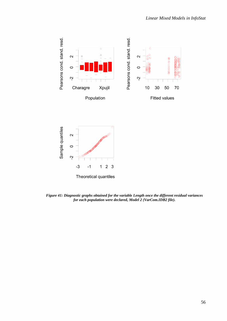
Linear Mixed Models in InfoStat
56
Figure 41: Diagnostic graphs obtained for the variable Length once the different residual variances
for each population were declared, Model 2 (VarCom.IDB2 file).

Linear Mixed Models in InfoStat
57
Crossed random effects with interaction
There are many situations in which the interest lies in estimating variance components
associated with two crossed factors and their interaction. Milliken and Johnson (1992, p.
265) present an example of efficiency in three production lines (randomly chosen in a
factory). Four operators were randomly chosen, and these operators worked in each of
the production lines. Originally each operator was supposed to work on each production
line five times, but for different reasons there are combinations which were repeated
fewer times (there are between one and five efficiency data for each operator-production
line combination).
Since both the production line and the operator are random, and we are also interested in
the additional variability generated by each specific combination, we are going to use a
model with two random effects and their interaction:
2 2
2 2
~ 0, , ~ 0,
~ 0, , ~ 0,
ijk i j ij ijk
i a j b
ij ab ijk e
Y a b ab e
a N b N
ab N e N
(6)
where all the random effects are mutually independent.
In order to fit this model we will use the dataset Production.IDB2 (Milliken and
Johnson, 1992). Efficiency is indicated in the Variables window, Production Line and
Operator are selected in the Class variables window. Since there is no fixed effect
(except the general mean), nothing is selected in the Fixed effects tab. In the Random
effects tab we select Production Line and Operator, and the option Crossed random
factors and interactions appears after clicking the right mouse with both variables
selected. In order to simplify the interpretation of the output (remember that the main
goal in this type of models is the estimation of variance components), we have
unchecked the option Standard deviations relative to residual standard deviation Figure
42.

Linear Mixed Models in InfoStat
58
Figure 42: Window displaying the Random effects tab with Line and Operator effects crossed and their
interaction, file Production.IDB2.
Extended and mixed linear models
R specification of the model
model.000_Efficiency_REML<-lme(Efficiency~1
,random=list(.U.=pdBlocked(list(pdIdent(~Production.line-1)
,pdIdent(~Operator-1)
,pdIdent(~Production.line:Operator-1))))
,method="REML"
,control=lmeControl(msMaxIter=200)
,na.action=na.omit
,data=R.data00
,keep.data=FALSE)
Results for model: model.000_Efficiency_REML
Dependent variable: Efficiency
Fit measurements
N AIC BIC logLik Sigma R2_0 R2_1
47 249.64 258.78 -119.82 1.99 0.95 Smaller AIC and BIC is better

Linear Mixed Models in InfoStat
59
Sequential hypothesis testing
numDF denDF F-value p-value
(Intercept) 1 46 478.29 <0.0001
Fixed effects
Value Std.Error DF t-value p-value
(Intercept) 83.38 3.81 46 21.87 <0.0001
Random effects parameters
Covariance model for random effects: pdBlocked
Formula: ~Production.line + Operator + Production.line:Operator - 1
Standard deviations and correlations
S.D.
Production.line1 5.67
Production.line2 5.67
Production.line3 5.67
Operator1 1.74
Operator2 1.74
Operator3 1.74
Operator4 1.74
Production.line1:Operator1.. 5.96
Production.line2:Operator1.. 5.96
Production.line3:Operator1.. 5.96
Production.line1:Operator2.. 5.96
Production.line2:Operator2.. 5.96
Production.line3:Operator2.. 5.96
Production.line1:Operator3.. 5.96
Production.line2:Operator3.. 5.96
Production.line3:Operator3.. 5.96
Production.line1:Operator4.. 5.96
Production.line2:Operator4.. 5.96
Production.line3:Operator4.. 5.96
From this output we note that the standard deviation estimates for each random effect
are:
ˆ ˆ ˆ ˆ5.6672, 1.7353, 5.9618, 1.9947a b ab e
This information can be used, for example, to estimate different types of intraclass
correlations. For example, the correlation between two observations from the same
production line and operator is:

Linear Mixed Models in InfoStat
60
2 2 2'
' 2 2 2 2
2 2 2
2 2 2 2
cov , ˆ ˆ ˆcorr ,
ˆ ˆ ˆ ˆvar
5.6672 1.7353 5.96180.9467
5.6672 1.7353 5.9618 1.9947
ijk ijk a b abijk ijk
a b ab eijk
Y YY Y
Y
On the other hand, the correlation between two observations from the same operator but
in different production lines is much smaller:
' '
' '
2 2
2 2 2 2 2 2 2 2
cov ,corr ,
var
ˆ 1.73530.0403.
ˆ ˆ ˆ ˆ 5.6672 1.7353 5.9618 1.9947
ijk i jk
ijk i jk
ijk
b
a b ab e
Y YY Y
Y

Linear Mixed Models in InfoStat
61
Application of mixed models for hierarchical data
Split plots
Let us suppose a two-factor experiment is performed, in which it is not possible to
randomly assign the combinations of both factors to the experimental plots (EP). In
some cases, groups of EP randomly receive the different levels of one of the
classification factors, and within these plot groups, the levels of the second factors are
randomly assigned.
The experiment previously described differs from a conventional two-factor experiment
in that, although the levels of the factors are randomly assigned to the EP, the treatments
(i.e., the combinations of the factors levels) are not the assigned in this way.
This particular way of assigning the different levels of the factors to the plots represents
a restriction to the randomization, and it induces correlation structures that should be
taken into account in the analysis. This is known as the split plot design.
The name emerges from the idea that the main PLOTS receive the levels of a factor
(sometimes also called main factor) and that these plots are SPLIT into SUBPLOTS,
which receive the levels of the second classification factor.
Although in the split plots the factors of a level are assigned within the levels of another
factor, this is NOT a nested design. It consists of a typical factorial experiment in which
the factors are crossed. It is only the randomization that has been done in a sequential
way.
Depending on the arrangement of the main plots, the design can be of:
• Split plots arranged in a randomized complete block design (RCBD).
• Split plots in a completely randomized design
• Split plots arranged in other designs
Split plots arranged in a RCBD
The classical analysis of a split plots design with the main plots arranged in complete
blocks includes the following terms in the model:

Linear Mixed Models in InfoStat
62
Factor associated with the main plot (MPF)
Block
Block*MPF (main plot error)
Factor associated with the subplot (SPF)
MPF*SPF
Error (error for the subplot)
The key point to perform the analysis of this model is to understand that the
experimental error for MPF is different from the terms of the model that include the
SPF. The experimental error of the main plots is generally larger than that of the
subplots.
The experimental error variance of the main plots in a split-plot design with main plots
arranged in a randomized complete block design, is estimated as the mean square (MS)
of the interaction Block*MPF (assuming that there is no interaction Block*MPF, and
consequently this MS estimates the error between main plots treated in the same way).
The MS of this “interaction” is used as a reference point to calculate the F statistic of
the hypothesis test for the main factor. For the rest of the tests, the residual MS is used
to construct the F statistic.
The analysis of this design by means of a linear mixed model is based on the
identification of two grouping levels for the response variable. The first level is given
by the blocks, and the second level is given by the main plots within the blocks. Each
one of these grouping levels generates a correlation, known as intra-class correlation,
among the observations it contains.
The mixed linear model for this design is the following:
; 1,.., ; 1,..., ; 1,...,ijk i j ij k ik ijky b p i T j G k B (7)
where ijky represents the response variable in the k-th block, in the i-th level of the
principal factor, and in the j-th level of the factor associated with the sub-plots;
represents the general mean of the response; i represents the effect of the i-th level of
the factor associated with the main plot; j represents the effect of the j-th level of the

Linear Mixed Models in InfoStat
63
factor associated with the subplots; and ij represents the effect of the interaction of the
ij-th treatment. On the other hand kb , ikp and ijk correspond to the random effects of
the blocks, the plots within the blocks and the experimental errors, respectively. The
assumptions for these random components are as follows: 2~ 0,k bb N ,
2~ 0,ik pp N , 2~ 0,ijk N , and that these three random components are
independent. Below we exemplify the analysis of a split plot design with blocks through
the use of a mixed linear model.
In this example (Di Rienzo 2007), four varieties of wheat are evaluated: BUCK-Charrua
(BC), Las Rosas-INTA (LI), Pigué (Pe), and Pro-INTA Puntal (PP), irrigated and rain-
fed with the field design shown in Figure 43.
Block 1 BC Pe PP LI
LI BC Pe PP
Block 2 PP BC Pe LI
PP Pe LI BC
Block 3 Pe LI BC PP
BC PP Pe LI
Figure 43: Scheme of the split plots design for the example (Wheat.IDB2 file, light gray =irrigation,
dark gray=rainfed).
The data in this example can be found in the Wheat.IDB2 file. The following is the
heading for the data table (Figure 44).
Figure 44: Heading of the data table (Wheat.IDB2 file).

Linear Mixed Models in InfoStat
64
The factor in the main plot is Water, the factor associated with the subplots is Variety,
and the response variable is Yield. The blocks are clearly identified, but the main plots
are not shown explicitly. This is so because in a split-plot design, the main plots within
a block are confounded with the main factor. Thus, the observations under Irrigation in
block 1 represent the observations of one of the main plots of this block.
To analyze this example we request the estimation of a mixed linear model. This
generates the variables selection window. Figure 45 shows the appropriate selection of
response variables and factors
Figure 45: Variables selection window for Extended and mixed linear models (Wheat.IDB2 file).
Upon accepting this specification, the dialogue to specify the model appears. The tab for
the fixed part, which has already been specified, is shown in Figure 46. Here the main
effects Water, Variety and the interaction Water*Variety appear.

Linear Mixed Models in InfoStat
65
Figure 46: Window displaying the Fixed effects tab (Wheat.IDB2 file).
For the specification of the random part, first the random factor Block and then the
factor Water are incorporated into the Random effects tab. This is how to indicate that
Water is within Block. The specification of the random part should be as shown in
Figure 47.

Linear Mixed Models in InfoStat
66
Figure 47: Window displaying the Random effects tab, with Block and Water as stratification criteria
(Wheat.IDB2 file).
The following output corresponds to this estimation:
Extended and mixed linear models
R specification of the model
model000_Performance_REML<-
lme(Performance~1+Water+Variety+Water:Variety
,random=list(Block=pdIdent(~1)
,Water=pdIdent(~1))
,method="REML"
,na.action=na.omit
,data=R.data00
,keep.data=FALSE)
Results for model: model000_Performance_REML
Dependent variable:Performance
Fit measurements
N AIC BIC logLik Sigma R2_0 R2_1 R2_2
24 206.59 215.09 -92.30 51.65 0.84 0.89 0.91 Smaller AIC and BIC is better

Linear Mixed Models in InfoStat
67
Sequential hypothesis testing
numDF denDF F-value p-value
(Intercept) 1 12 363.93 <0.0001
Water 1 2 55.24 0.0176
Variety 3 12 6.38 0.0078
Water:Variety 3 12 2.36 0.1223
Random effects parameters
Covariance model for random effects: pdIdent
Formula: ~1|Block
Standard deviations relative to residual standard deviation and
correlation
(const)
(const) 0.55
Covariance model for random effects: pdIdent
Formula: ~1|Water in Block
Standard deviations relative to residual standard deviation and
correlation
(const)
(const) 0.47
In this problem, sequential hypothesis tests are equivalent to marginal tests because the
data are balanced.
Before continuing with our analysis, we will validate some of the assumptions of the
models by reviewing standardized residuals vs. predicted values and other classification
criteria as well as the normal Q-Q plot for standardized residuals. These residuals are
conditional on the random effects (in other words, they approximate the errors). To do
so, we will select the Model exploration submenu. In the dialogue window, we will
select the Diagnostic tab, and then select the Residuals vs. subtab (Figure 48).

Linear Mixed Models in InfoStat
68
Figure 48: Model exploration window for the comparison of extended and mixed models displaying the
Diagnostic tab (Wheat.IDB2 file).
If the items are selected from the available list, as shown in Figure 48, the graph shown
below will be obtained (Figure 49). This is shown in a new window that R generates,
and its content can be copied by right clicking on the image. In the displayed menu, the
options “Copy as metafile” or “Copy as bitmap” are available.
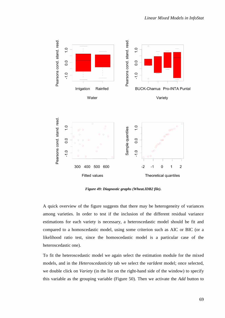
Linear Mixed Models in InfoStat
69
Figure 49: Diagnostic graphs (Wheat.IDB2 file).
A quick overview of the figure suggests that there may be heterogeneity of variances
among varieties. In order to test if the inclusion of the different residual variance
estimations for each variety is necessary, a heteroscedastic model should be fit and
compared to a homoscedastic model, using some criterion such as AIC or BIC (or a
likelihood ratio test, since the homoscedastic model is a particular case of the
heteroscedastic one).
To fit the heteroscedastic model we again select the estimation module for the mixed
models, and in the Heteroscedasticity tab we select the varIdent model; once selected,
we double click on Variety (in the list on the right-hand side of the window) to specify
this variable as the grouping variable (Figure 50). Then we activate the Add button to

Linear Mixed Models in InfoStat
70
make the incorporation of this model specification effective. If for some reason the
specification is not wanted, the user can erase it by double clicking on it.
Figure 50: Window displaying the Heteroscedasticity tab, with the varIdent function with Variety
selected as a grouping variable (Wheat.IDB2 file).
The fitted measures for the specified model are as follows
Measures of model fit
N AIC BIC logLik Sigma R2_0 R2_1 R2_2
24 209.47 220.28 -90.73 24.49 0.84 0.89 0.90 AIC and BIC smaller means better
Compared to the fitted measures for the homoscedastic model an improvement is not
observed; on the other hand, both AIC and BIC increased. Therefore, the
heteroscedastic model is rejected.

Linear Mixed Models in InfoStat
71
Returning to the homoscedastic model, we will make multiple comparisons of Fisher’s
LSD in order to evaluate the differences between the varieties. To do so, in the
Comparisons tab, in the Means subtab, we check the Variety option, as shown in Figure
51.
Figure 51: Window displaying the Comparisons tab, and the selection of the Means subtab
(Wheat.IDB2 file).
At the end of the output there is a means comparison. Note that only BUCK-Charrua
had the lowest yields, and this occurred independently of whether it had irrigation.
Meanwhile, other varieties had statistically indistinguishable yields.
Adjusted means and standard error for Variety
LSD Fisher (alpha=0.05)
p-value correction procedure: No
Variety Means S.E.
Pro-INTA Puntal 469.50 46.28 A
Pigue 430.98 28.77 A
LasRosas-INTA 423.98 33.74 A
BUCK-Charrua 342.73 29.38 B Means with a common letter are not significantly different (p<= 0.05)

Linear Mixed Models in InfoStat
72
Split plots in a completely randomized design
The following example comes from an experiment whose objective was to evaluate the
effect of an adjuvant on the drops coverage and on the
uniformity of application on different locations of the
leaves in the canopy of a soy crop (Di Rienzo 2007).
Sixteen sites where selected, in each of which 4 hydro-
sensitive cards where located at two heights of the
canopy (upper and lower), with their sensitive face
pointing in one of two directions (abaxial and axial).
The hydro-sensitive cards show a spot on the location
where a drop of water falls. The stained surface of
these cards is a measure of how much water penetrates
and disperses in a given zone of the canopy. In 8 of the
16 sites, an adjuvant was added to the pulverized water
(to diminish the surface water tension and improve the dispersion of the drops), and in
the remaining 8 no adjuvant was added. Thus, at each pulverization site 4 records are
obtained that correspond to the combination of heights (upper and lower) and the
direction of the sensitive face of the cards (abaxial and axial). Then at each site there is
a complete repetition of an experiment with 4 treatments (upper-abaxial, lower-abaxial,
upper-axial and lower-axial), combined with the presence or absence of the adjuvant in
the sprayed solution.
The resulting experiment is tri-factorial, with a main factor (adjuvant) associated with
the main plots (sites where the spraying is done), and two factors (height and direction
of the sensitive side of the card) associated with the subplots (cards within the site). The
file containing the data is called Coverage drops.IDB2 and the heading of the data table
is shown in Figure 52.

Linear Mixed Models in InfoStat
73
Figure 52: Heading of the data table (Coverage drops.IDB2 file).
In the data table there is a column that identifies the plot; it is numbered from 1 to 16.
This is going to be the only random effect in our model (besides the error term, which is
always present).
The linear model for the observations of this experiment is as follows:
;
1,.., 2; 1,..., 2; 1,..., 2; 1,...,16
ijkl i j k ij ik jk ijk l ijkly p
i j k l
(8)
where ijkly represents the response variable (Coverage) in the i-th level of the Adjuvant
factor, in the j-th level of the Height factor, in the k-th level of the Face factor, and in
the l-th Plot; represents the general mean of the response; i represents the effect of
the i-th level of the factor associated with the main plots (Adyuvant); j represents the
effect of the j-th level of the Height factor; and k represents the k-th level of the Face
factor, both of which are associated with the subplots; and ij , ik ,
jk y ijk are the
interactions of the second and third order corresponding to the Adjuvant, Height and
Face factors. Furthermore, lb and ijkl represent the random effect of the plots and
experimental errors, respectively. The assumptions about these random components are
that 2~ 0,l bb N , that 2~ 0,ijkl N , and that these two random components are
independent. Next we show how the previous model is specified in InfoStat, the output,
an interpretation and some complementary actions for the validation of the model. For
this, we select the Extended and mixed linear models >>Model estimation menu. The
variable selection dialogue for this case is shown in Figure 53.

Linear Mixed Models in InfoStat
74
Figure 53: Variables selection window for Extended and mixed linear models (Coverage drops.IDB2
file).
The specification of the fixed part of the model in this example contains the three
factors and the double and triple interactions (Figure 54).
Figure 54: Window displaying the Fixed effects tab (Coverage drops.IDB2 file).

Linear Mixed Models in InfoStat
75
The random effect considered in this example is Plot (Figure 55).
Figure 55: Window displaying the Random effects tab, with Plot as the stratification criterion
(Coverage drops.IDB2 file).
After accepting the previous specifications, we obtain the following output:
Extended and mixed linear models
R specification of the model
model000_Coverage_REML<-
lme(Coverage~1+Adjuvant+Height+Face+Adjuvant:Height+Adjuvant:Face+Heig
ht:Face+Adjuvant:Height:Face
,random=list(Plot=pdIdent(~1))
,method="REML"
,na.action=na.omit
,data=R.data00
,keep.data=FALSE)
Results for model: model000_Coverage_REML
Dependent variable:Coverage
Fit measurements
N AIC BIC logLik Sigma R2_0 R2_1
64 670.38 690.63 -325.19 65.17 0.76 0.82 Smaller AIC and BIC is better

Linear Mixed Models in InfoStat
76
Sequential hypothesis testing
numDF denDF F-value p-value
(Intercept) 1 42 233.37 <0.0001
Adjuvant 1 14 1.89 0.1909
Height 1 42 72.86 <0.0001
Face 1 42 95.32 <0.0001
Adjuvant:Height 1 42 1.58 0.2152
Adjuvant:Face 1 42 0.01 0.9271
Height:Face 1 42 34.77 <0.0001
Adjuvant:Height:Face 1 42 0.21 0.6476
Random effects parameters
Covariance model for random effects: pdIdent
Formula: ~1|Plot
Standard deviations relative to residual standard deviation and
correlation
(const)
(const) 0.40
A revision of the standardized residuals of this model using the diagnostic tools in the
Extended and mixed linear models >> Model exploration menu shows that
heterogeneity of variances may exist when we compare the residuals for both faces
(abaxial and axial) of the hydro-sensitive card (Figure 56).

Linear Mixed Models in InfoStat
77
Figure 56: Box plots for the Pearson standardized residuals for the levels of the factor Face.
In order to take into account the heterogeneity of variances, we will again select the
model estimation menu. All of the previous specifications have been kept, which is why
we need only concentrate on the specification of the variance model. To do so, we use
the Heteroscedasticity tab as shown in Figure 57.

Linear Mixed Models in InfoStat
78
Figure 57: Window displaying the Heteroscedasticity tab, with Face as a grouping variable (Coverage
drops.IDB2 file).
The resulting output is as follows:
Extended and mixed linear models
R specification of the model
model002_Coverage_REML<-
lme(Coverage~1+Adjuvant+Height+Face+Adjuvant:Height+Adjuvant:Face+Heig
ht:Face+Adjuvant:Height:Face
,random=list(Plot=pdIdent(~1))
,weight=varComb(varIdent(form=~1|Face))
,method="REML"
,na.action=na.omit
,data=R.data00
,keep.data=FALSE)
Results for model: model002_Coverage_REML
Dependent variable:Coverage
Fit measurements
N AIC BIC logLik Sigma R2_0 R2_1
64 636.54 658.82 -307.27 21.26 0.76 0.81 Smaller AIC and BIC is better

Linear Mixed Models in InfoStat
79
Sequential hypothesis testing
numDF denDF F-value p-value
(Intercept) 1 42 176.66 <0.0001
Adjuvant 1 14 4.19 0.0599
Height 1 42 53.72 <0.0001
Face 1 42 98.43 <0.0001
Adjuvant:Height 1 42 13.83 0.0006
Adjuvant:Face 1 42 0.01 0.9259
Height:Face 1 42 35.90 <0.0001
Adjuvant:Height:Face 1 42 0.22 0.6423
Random effects parameters
Covariance model for random effects: pdIdent
Formula: ~1|Plot
Standard deviations relative to residual standard deviation and
correlation
(const)
(const) 1.06
Variance structure
Variance model: varIdent
Formula: ~ 1 | Face
Variance-function parameters
Parameter Estim.
Abaxial 1.00
Axial 4.15
The model for this data would be ijkl i jk l ijkly p , where i jk represents the fixed
effect of the i-th Adjuvant, j-th Height and k-th Face (Axial or Abaxial), lb is the random
effect of l-th experimental plot experimental that is assumed 20, pN , and
2~ 0,ijkl kN . The variance of an observation taken from a randomly selected plot
will depend on whether the observation is taken from a card facing the Axial or Abaxial
direction. Thus, if we take an observation from an Abaxial face, the variance is
(21.26*1.06)2 + (21.26*1)2, and if we take the observation from an Axial face it is
(21.26*1.06)2 + (21.26*4.15)2.
The summary statistics for the homoscedastic and heteroscedastic models are shown
below.
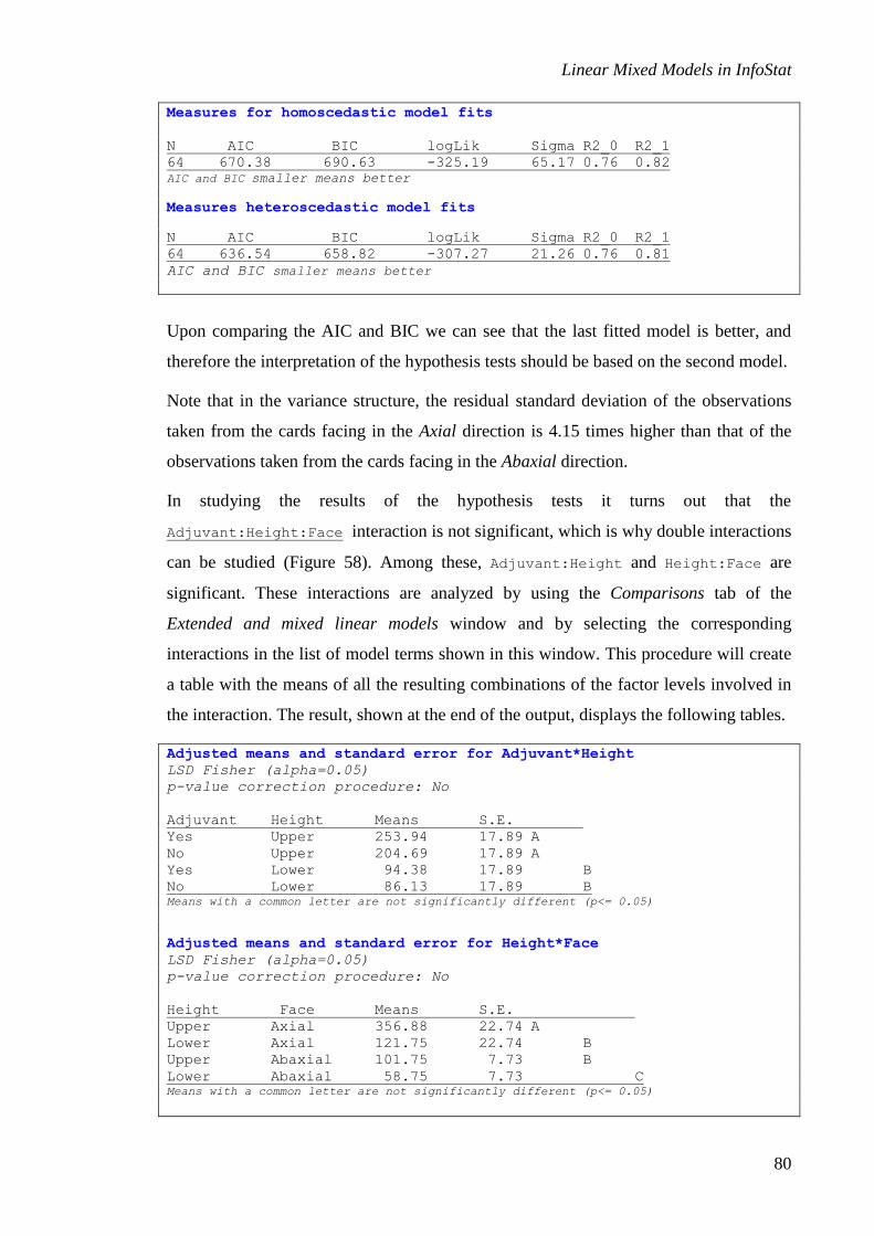
Linear Mixed Models in InfoStat
80
Measures for homoscedastic model fits
N AIC BIC logLik Sigma R2_0 R2_1
64 670.38 690.63 -325.19 65.17 0.76 0.82
AIC and BIC smaller means better
Measures heteroscedastic model fits
N AIC BIC logLik Sigma R2_0 R2_1
64 636.54 658.82 -307.27 21.26 0.76 0.81
AIC and BIC smaller means better
Upon comparing the AIC and BIC we can see that the last fitted model is better, and
therefore the interpretation of the hypothesis tests should be based on the second model.
Note that in the variance structure, the residual standard deviation of the observations
taken from the cards facing in the Axial direction is 4.15 times higher than that of the
observations taken from the cards facing in the Abaxial direction.
In studying the results of the hypothesis tests it turns out that the
Adjuvant:Height:Face interaction is not significant, which is why double interactions
can be studied (Figure 58). Among these, Adjuvant:Height and Height:Face are
significant. These interactions are analyzed by using the Comparisons tab of the
Extended and mixed linear models window and by selecting the corresponding
interactions in the list of model terms shown in this window. This procedure will create
a table with the means of all the resulting combinations of the factor levels involved in
the interaction. The result, shown at the end of the output, displays the following tables.
Adjusted means and standard error for Adjuvant*Height
LSD Fisher (alpha=0.05)
p-value correction procedure: No
Adjuvant Height Means S.E.
Yes Upper 253.94 17.89 A
No Upper 204.69 17.89 A
Yes Lower 94.38 17.89 B
No Lower 86.13 17.89 B Means with a common letter are not significantly different (p<= 0.05)
Adjusted means and standard error for Height*Face
LSD Fisher (alpha=0.05)
p-value correction procedure: No
Height Face Means S.E.
Upper Axial 356.88 22.74 A
Lower Axial 121.75 22.74 B
Upper Abaxial 101.75 7.73 B
Lower Abaxial 58.75 7.73 C Means with a common letter are not significantly different (p<= 0.05)

Linear Mixed Models in InfoStat
81
a) b)
Figure 58: Dot plot for the study of the interaction between Adjuvant and Height (a) and between Face
and Height (b).
Split-split plot
This design is based on the same principle as the split plots, but it expands it a step
further. The principle can be arbitrarily extended to deeper levels of division. The linear
model for this design, assuming that the main plots are grouped in randomized complete
blocks, is the following:
ijkl i j k ij ik jk ijk l il jil ijkly b p sp (9)
In the previous expression represents the general mean; i represents the i-th level
of the factor associated with the main plots; j represents the j-th level of the factor
associated with the subplots within the main plots; k represents the k-th level of the
factor associated with the subplots (within the subplots); and ij , ik , jk y ijk represents
the corresponding interactions. The random terms of this model correspond to the
effects of the blocks, 2~ 0,l bb N , the effects of the plots, 2~ 0,il pp N , the effects
of the sub-plots, 2~ 0,jil spsp N , and the experimental error, 2~ 0,ijkl N . All of
them, as usual, are assumed to be independent.
Let us now consider an example. The data are in the Starch quality.IDB2 file (Di Rienzo
2007). In this experiment, we evaluate the water absorption index (WAI) of cooked and
raw starch of two genotypes of Quinoa (Chenopodium quinoa) cultivated under 4 levels
Adjuvant-No Adjuvant-Yes
Upper Low er
Height
0
50
100
150
200
250
300
Co
ve
rag
e
Adjuvant-No Adjuvant-Yes Face-Abaxial Face-Axial
Upper Low er
Height
0
100
200
300
400
Co
ve
rag
e
Face-Abaxial Face-Axial
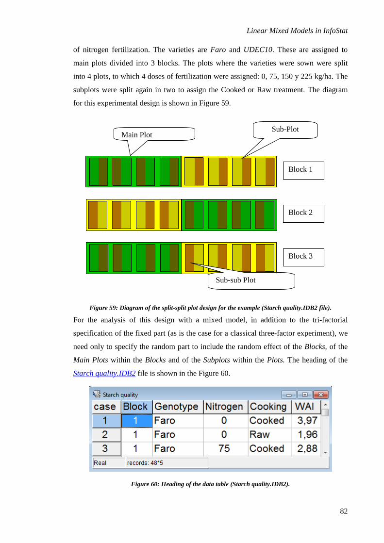
Linear Mixed Models in InfoStat
82
of nitrogen fertilization. The varieties are Faro and UDEC10. These are assigned to
main plots divided into 3 blocks. The plots where the varieties were sown were split
into 4 plots, to which 4 doses of fertilization were assigned: 0, 75, 150 y 225 kg/ha. The
subplots were split again in two to assign the Cooked or Raw treatment. The diagram
for this experimental design is shown in Figure 59.
Figure 59: Diagram of the split-split plot design for the example (Starch quality.IDB2 file).
For the analysis of this design with a mixed model, in addition to the tri-factorial
specification of the fixed part (as is the case for a classical three-factor experiment), we
need only to specify the random part to include the random effect of the Blocks, of the
Main Plots within the Blocks and of the Subplots within the Plots. The heading of the
Starch quality.IDB2 file is shown in the Figure 60.
Figure 60: Heading of the data table (Starch quality.IDB2).
Block 1
Block 2
Block 3
Sub-sub Plot
Sub-Plot
Main Plot
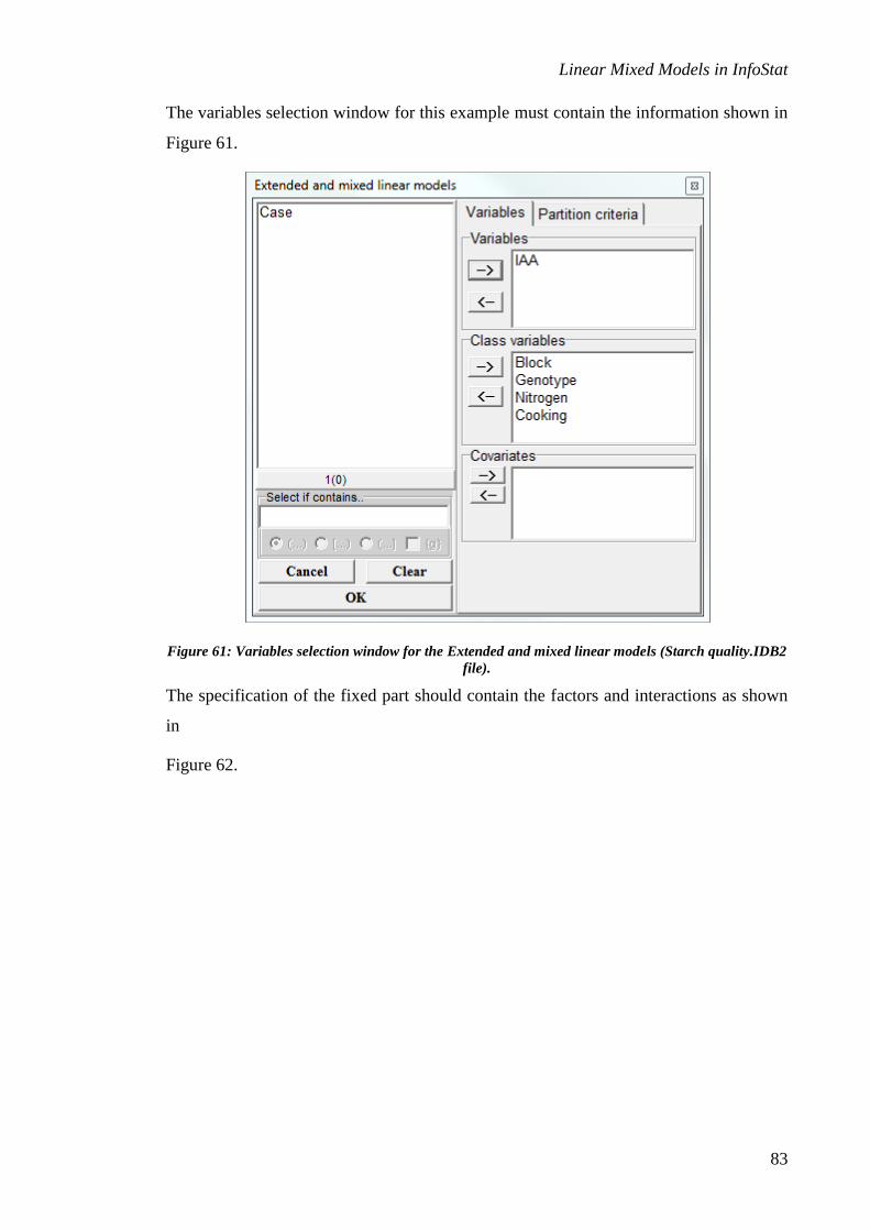
Linear Mixed Models in InfoStat
83
The variables selection window for this example must contain the information shown in
Figure 61.
Figure 61: Variables selection window for the Extended and mixed linear models (Starch quality.IDB2
file).
The specification of the fixed part should contain the factors and interactions as shown
in
Figure 62.
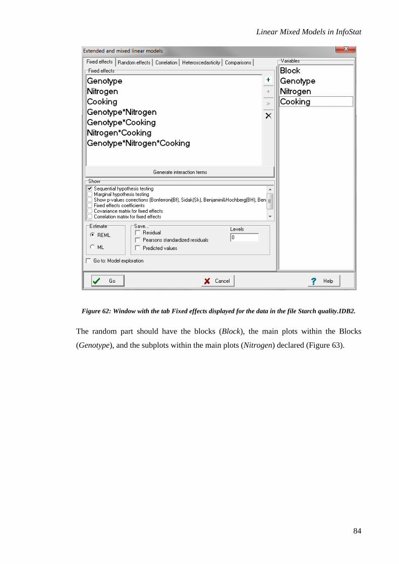
Linear Mixed Models in InfoStat
84
Figure 62: Window with the tab Fixed effects displayed for the data in the file Starch quality.IDB2.
The random part should have the blocks (Block), the main plots within the Blocks
(Genotype), and the subplots within the main plots (Nitrogen) declared (Figure 63).

Linear Mixed Models in InfoStat
85
Figure 63: Window displaying the Random effects tab (Starch quality.IDB2 file).
The corresponding output is as follows:
Extended and mixed linear models
R specification of the model
model000_WAI_REML<-
lme(WAI~1+Genotype+Nitrogen+Cooking+Genotype:Nitrogen+Genotype:Cooking
+Nitrogen:Cooking+Genotype:Nitrogen:Cooking
,random=list(Block=pdIdent(~1)
,Genotype=pdIdent(~1)
,Nitrogen=pdIdent(~1))
,method="REML"
,na.action=na.omit
,data=R.data00
,keep.data=FALSE)
Results for model: model000_WAI_REML
Dependent variable:WAI

Linear Mixed Models in InfoStat
86
Fit measurements
N AIC BIC logLik Sigma R2_0 R2_1 R2_2 R2_3
48 116.45 145.76 -38.22 0.61 0.75 0.75 0.75 0.75 Smaller AIC and BIC is better
Sequential hypothesis testing
numDF denDF F-value p-value
(Intercept) 1 16 1389.20 <0.0001
Genotype 1 2 14.49 0.0626
Nitrogen 3 12 0.78 0.5287
Cooking 1 16 32.90 <0.0001
Genotype:Nitrogen 3 12 0.88 0.4769
Genotype:Cooking 1 16 37.67 <0.0001
Nitrogen:Cooking 3 16 1.74 0.1998
Genotype:Nitrogen:Cooking 3 16 0.46 0.7108
Random effects parameters
Covariance model for random effects: pdIdent
Formula: ~1|Block
Standard deviations relative to residual standard deviation and
correlation
(const)
(const) 1.3E-05
Covariance model for random effects: pdIdent
Formula: ~1|Genotype in Block
Standard deviations relative to residual standard deviation and
correlation
(const)
(const) 5.0E-06
Covariance model for random effects: pdIdent
Formula: ~1|Nitrogen in Genotype in Block
Standard deviations relative to residual standard deviation and
correlation
(const)
(const) 1.8E-05
We could continue to conduct diagnostic tests, but we will assume that the model is
correct. The interpretation of the hypothesis tests indicates that only the
Genotype:Cooking interaction is significant. The multiple comparisons for the means of
the corresponding treatments for this interaction are shown below. In these tests, note
that only the cooked starch of the UDEC10 genotype shows a WAI significantly higher
than that of the rest of the combinations of Genotype and Cooking.

Linear Mixed Models in InfoStat
87
Adjusted means and standard error for Genotype*Cooking
LSD Fisher (alpha=0.05)
p-value correction procedure: No
Genotype Cooking Means S.E.
UDEC10 Cooked 4.64 0.18 A
Faro Raw 2.97 0.18 B
Faro Cooked 2.90 0.18 B
UDEC10 Raw 2.56 0.18 B Means with a common letter are not significantly different (p<= 0.05)
An alternative way to formulate the previous model consists of leaving the fixed effects as shown in
Figure 62 and specifying the random effects as shown in Figure 64. The results are
exactly the same as before, except for the calculation of the degrees of freedom of the
denominator; therefore, the probability values are not the same. This approximation is
also valid, although the previous version is in line with the traditional analysis for
balanced data based on fixed effects. Note that the variance estimations are presented
differently.
Figure 64: Window displaying the Random effects tab that shows another way to specify the random
part (Starch quality.IDB2 file).
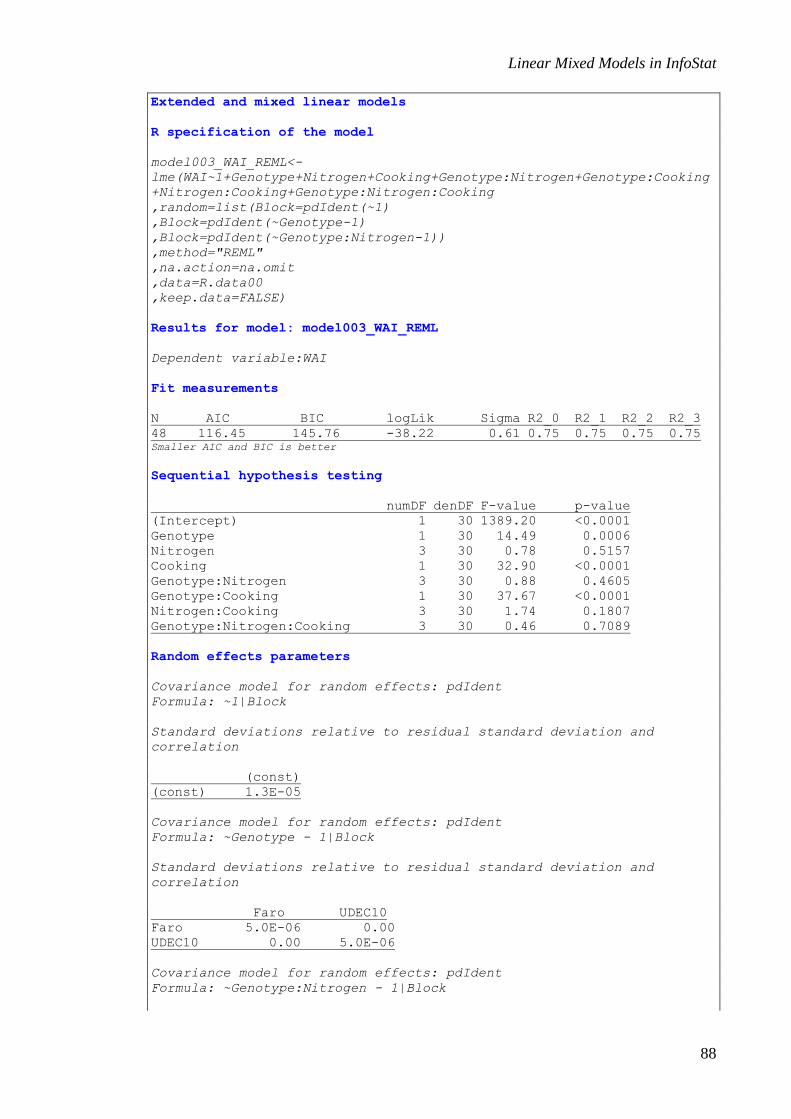
Linear Mixed Models in InfoStat
88
Extended and mixed linear models
R specification of the model
model003_WAI_REML<-
lme(WAI~1+Genotype+Nitrogen+Cooking+Genotype:Nitrogen+Genotype:Cooking
+Nitrogen:Cooking+Genotype:Nitrogen:Cooking
,random=list(Block=pdIdent(~1)
,Block=pdIdent(~Genotype-1)
,Block=pdIdent(~Genotype:Nitrogen-1))
,method="REML"
,na.action=na.omit
,data=R.data00
,keep.data=FALSE)
Results for model: model003_WAI_REML
Dependent variable:WAI
Fit measurements
N AIC BIC logLik Sigma R2_0 R2_1 R2_2 R2_3
48 116.45 145.76 -38.22 0.61 0.75 0.75 0.75 0.75 Smaller AIC and BIC is better
Sequential hypothesis testing
numDF denDF F-value p-value
(Intercept) 1 30 1389.20 <0.0001
Genotype 1 30 14.49 0.0006
Nitrogen 3 30 0.78 0.5157
Cooking 1 30 32.90 <0.0001
Genotype:Nitrogen 3 30 0.88 0.4605
Genotype:Cooking 1 30 37.67 <0.0001
Nitrogen:Cooking 3 30 1.74 0.1807
Genotype:Nitrogen:Cooking 3 30 0.46 0.7089
Random effects parameters
Covariance model for random effects: pdIdent
Formula: ~1|Block
Standard deviations relative to residual standard deviation and
correlation
(const)
(const) 1.3E-05
Covariance model for random effects: pdIdent
Formula: ~Genotype - 1|Block
Standard deviations relative to residual standard deviation and
correlation
Faro UDEC10
Faro 5.0E-06 0.00
UDEC10 0.00 5.0E-06
Covariance model for random effects: pdIdent
Formula: ~Genotype:Nitrogen - 1|Block

Linear Mixed Models in InfoStat
89
Standard deviations relative to residual standard deviation and
correlation
Faro:0 UDEC10:0 Faro:75 UDEC10:75 Faro:150 UDEC10:150 Faro:225 UDEC10:225
Faro:0 1.8E-05 0 0 0 0 0 0 0
UDEC10:0 0 1.8E-05 0 0 0 0 0 0
Faro:75 0 0 1.8E-05 0 0 0 0
UDEC10:75 0 0 0 1.8E-05 0 0 0 0
Faro:150 0 0 0 0 1.8E-05 0 0 0
UDEC10:150 0 0 0 0 0 1.8E-05 0 0
Faro:225 0 0 0 0 0 0 1.8E-05 0
UDEC10:225 0 0 0 0 0 0 0 1.8E-05

Linear Mixed Models in InfoStat
90
Application of mixed models for repeated measures in time
Longitudinal data
When modeling longitudinal data, the most important aspect to consider is the structure
of the residual covariance matrix, which can be modeled by specifying the correlation
matrix. In some cases, the variances can also be different for some grouping criterion
and heteroscedasticity should be modeled. Let us recall that there is a residual
correlation between observations that share the same value of the stratification criterion,
also known as subject (for example, observations taken over the same person, same
plot, same animal, same tree, etc.). Thus, the residual covariance matrix for all the
observations will be a block diagonal matrix by blocks, and in each block the desired
structure will be reflected, i.e. compound symmetry, first-order autoregressive, etc.
To specify this, InfoStat has two tabs. In the Correlation tab, options that allow the
specification of the error correlation structure can be found, and in the
Heteroscedasticity tab different variance models can be selected. Thus, the different
possible structures of the residual covariance matrix that can be fitted result from the
combination of the different correlation structures with potential heteroscedasticity in
time. If the researcher also wishes to specify a random effect, it is also possible to do so
by using the corresponding tab. In this case much caution should be taken to avoid
combining random effects, correlation structures and heteroscedasticity such that the
final model is not identifiable. This occurs when there is an infinite set of values for the
parameters for which the model is indistinguishable, and therefore the solutions to the
likelihood equations are not unique.
Examples of these situations occur when the user specifies both a compound symmetry
correlation structure with a stratification criterion (for example, the plot) and a random
effect of the same stratification criterion on the constant. In this case the covariance
structure of the observations will be a diagonal matrix by blocks, and each block will
have a compound symmetry structure. Therefore, this structure intrinsically has two
parameters. However, because of the way in which we have specified the structure,
three parameters are shown (random effect variance, intra-class correlation of the
residual correlation structure, and residual variance). This overparameterization creates
infinite solutions, and consequently the estimators cannot be interpreted (and in many
cases the numerical algorithm does not converge). Another common phenomenon is a
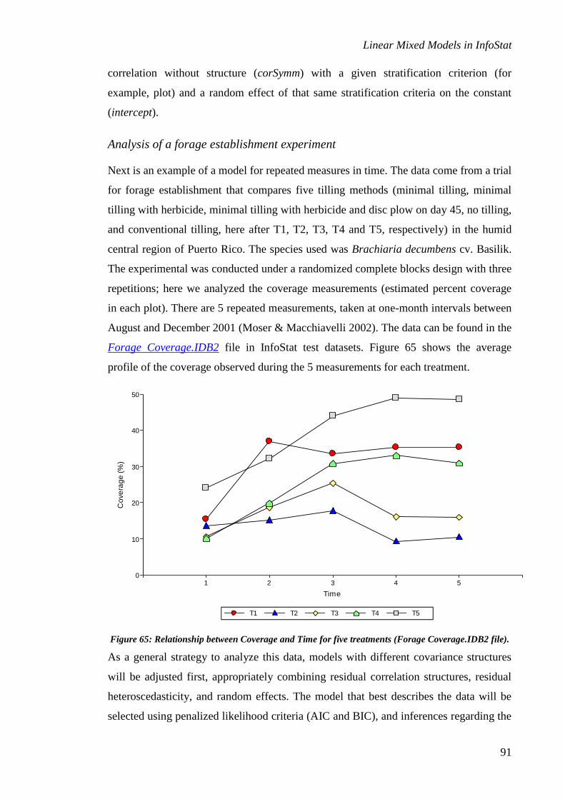
Linear Mixed Models in InfoStat
91
correlation without structure (corSymm) with a given stratification criterion (for
example, plot) and a random effect of that same stratification criteria on the constant
(intercept).
Analysis of a forage establishment experiment
Next is an example of a model for repeated measures in time. The data come from a trial
for forage establishment that compares five tilling methods (minimal tilling, minimal
tilling with herbicide, minimal tilling with herbicide and disc plow on day 45, no tilling,
and conventional tilling, here after T1, T2, T3, T4 and T5, respectively) in the humid
central region of Puerto Rico. The species used was Brachiaria decumbens cv. Basilik.
The experimental was conducted under a randomized complete blocks design with three
repetitions; here we analyzed the coverage measurements (estimated percent coverage
in each plot). There are 5 repeated measurements, taken at one-month intervals between
August and December 2001 (Moser & Macchiavelli 2002). The data can be found in the
Forage Coverage.IDB2 file in InfoStat test datasets. Figure 65 shows the average
profile of the coverage observed during the 5 measurements for each treatment.
Figure 65: Relationship between Coverage and Time for five treatments (Forage Coverage.IDB2 file).
As a general strategy to analyze this data, models with different covariance structures
will be adjusted first, appropriately combining residual correlation structures, residual
heteroscedasticity, and random effects. The model that best describes the data will be
selected using penalized likelihood criteria (AIC and BIC), and inferences regarding the
T1 T2 T3 T4 T5
1 2 3 4 5
Time
0
10
20
30
40
50
Co
ve
rag
e (
%)
T1 T2 T3 T4 T5

Linear Mixed Models in InfoStat
92
means (comparing treatments, studying the effect of time, analyzing whether the
average profiles vary in time, whether they are parallel, etc.) will be based on this
model.
To choose the best model we will start by proposing a simple model with few
parameters to estimate (i.e., parsimonious), and then we will add parameters until
finally considering the model without structure, which is the least parsimonious.
The following covariance structures will be used for the data (marginal covariance):
1. Random block effects and independent homoscedastic errors.
2. Random block and plot effects, and independent homoscedastic errors.
3. Random block effects and independent heteroscedastic errors.
4. Random block and plot effects, and independent heteroscedastic errors.
5. Random block effects, constant correlation within plots, and homoscedastic errors (equivalent to model 2).
6. Random block effects, constant correlation within plots, and heteroscedastic errors.
7. Random block effects, first-order autoregressive structure between errors of the same plot and homoscedastic errors.
8. Random block and plot effects, first-order autoregressive structure between errors of the same plot and homoscedastic errors.
9. Random block effects, first-order autoregressive structure between errors of the same plot and heteroscedastic errors.
10. Random block and plot effects, first-order autoregressive structure between errors of the same plot and heteroscedastic errors.
11. Random block effects, unstructured correlations between errors from the same plot and time-varying residual variances.
To fit these models, the variables should be specified as shown in Figure 66.

Linear Mixed Models in InfoStat
93
Figure 66: Variables selection window for Extended and mixed linear models (Forage Coverage.IDB2
file).
The same means model was used in every case, because the fixed part of the model did
not change (this is essential in order to compare covariance structures using REML, and
thus AIC and BIC criteria) (Figure 67). A way to declare each one of the models to be
evaluated is shown below, followed by the InfoStat output with the corresponding
fitness measures.

Linear Mixed Models in InfoStat
94
Figure 67: Window displaying the Fixed effects tab (Forage Coverage.IDB2 file).
Model 1: Random block effects and independent homoscedastic errors.
Select Block in the Random effects tab (Figure 68). In the Correlation tab the
Independent errors should be declared (Figure 69), which is the default option, and
nothing should be declared in the Heteroscedasticity tab.

Linear Mixed Models in InfoStat
95
Figure 68: Window displaying the Random effect tab for model 1(Forage Coverage.IDB2 file).

Linear Mixed Models in InfoStat
96
Figure 69: Window displaying the Correlation tab and the selection of Independent errors (Model 1)
(Forage Coverage.IDB2 file).
Fit measurements
N AIC BIC logLik Sigma R2_0 R2_1
75 476.39 528.01 -211.19 12.19 0.56 0.63 Smaller AIC and BIC is better
Model 2: Random block and plot effects, and independent homoscedastic errors.
Select Block and Plot in the Random effects tab (Figure 70). In the Correlation tab the
Independent errors should be declared (Figure 69), which is the default option, and
nothing should be declared in the Heteroscedasticity tab.

Linear Mixed Models in InfoStat
97
Figure 70: Window displaying the Random Effect tab, with Block and Plot selected (Model 2) (Forage
Coverage.IDB2 file).
Fit measurements
N AIC BIC logLik Sigma R2_0 R2_1 R2_2
75 470.00 523.54 -207.00 9.95 0.56 0.61 0.78 Smaller AIC and BIC is better
Model 3: Random block effects and independent heteroscedastic errors
The Random effect and Correlation tabs are specified as in model 1 (Figure 68 y Figure
69); in the Heteroscedasticity tab varIdent is specified; and Time is dragged in the
Grouping variables window (Figure 71).
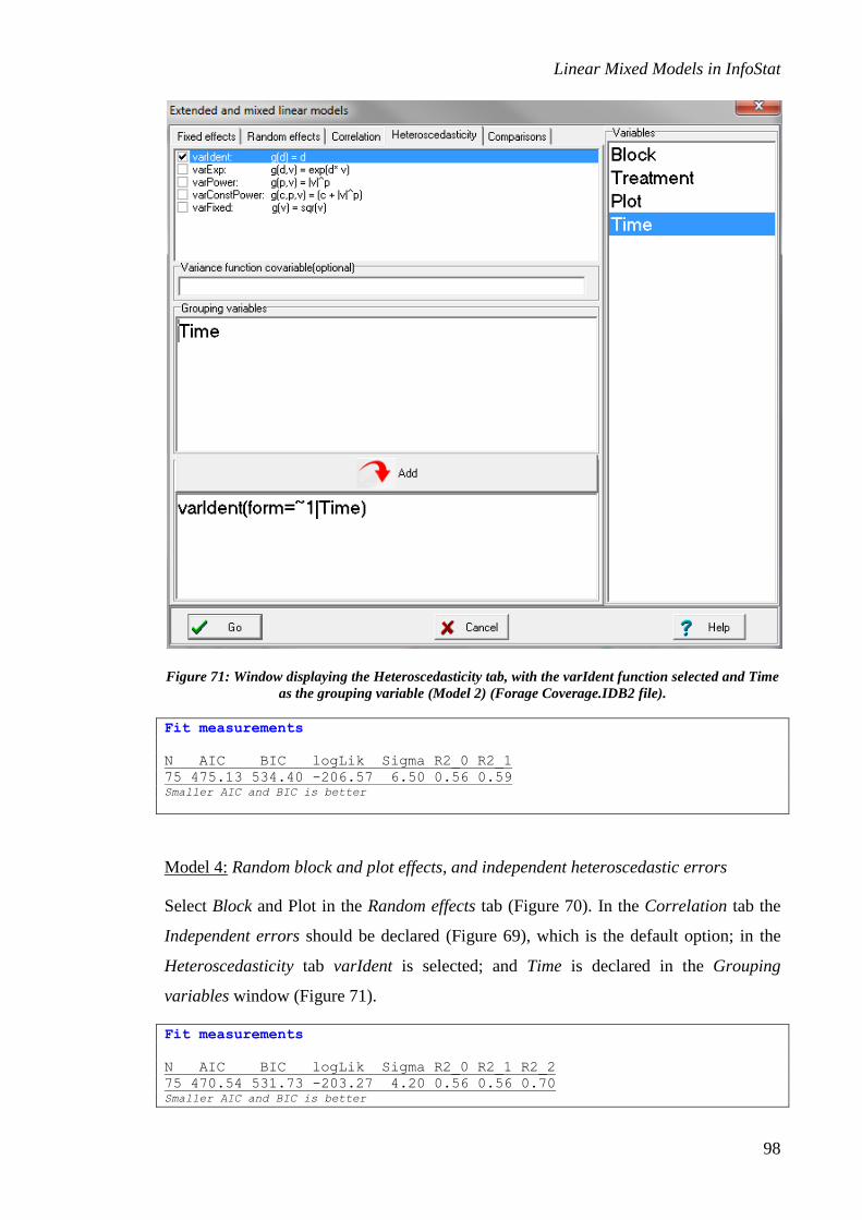
Linear Mixed Models in InfoStat
98
Figure 71: Window displaying the Heteroscedasticity tab, with the varIdent function selected and Time
as the grouping variable (Model 2) (Forage Coverage.IDB2 file).
Fit measurements
N AIC BIC logLik Sigma R2_0 R2_1
75 475.13 534.40 -206.57 6.50 0.56 0.59 Smaller AIC and BIC is better
Model 4: Random block and plot effects, and independent heteroscedastic errors
Select Block and Plot in the Random effects tab (Figure 70). In the Correlation tab the
Independent errors should be declared (Figure 69), which is the default option; in the
Heteroscedasticity tab varIdent is selected; and Time is declared in the Grouping
variables window (Figure 71).
Fit measurements
N AIC BIC logLik Sigma R2_0 R2_1 R2_2
75 470.54 531.73 -203.27 4.20 0.56 0.56 0.70 Smaller AIC and BIC is better

Linear Mixed Models in InfoStat
99
Model 5: Random block effects, constant correlation within plots, and homoscedastic
errors
In the Random effects tab Block is declared; in the Correlation tab the Compound
symmetry option is selected. In the Grouping variables window we should also specify
Block and Plot, so that it is explicitly stated the correlation of data coming from the
same plot and block is being modeled (Figure 72). In the Heteroscedasticity tab the
default option was kept, in other words, no criteria were selected (to do this, go to the
Heteroscedasticity tab and erase the previous selection by deactivating all the options
and erasing varIdent(form=~1) with a double click).
Figure 72: Window displaying the Correlation tab, and selection of Compound symmetry for data
grouped block and plot (Forage Coverage.IDB2 file).
Fit measurements
N AIC BIC logLik Sigma R2_0 R2_1
75 470.00 523.54 -207.00 12.59 0.56 0.61 Smaller AIC and BIC is better

Linear Mixed Models in InfoStat
100
Notice that this model yields the same value of –loglik, AIC, and BIC, because it is
essentially the same model (except in the case in which the constant correlation is
negative). Model 2 incorporates the correlation of observations in the same plot through
the random plot effect, while model 5 does this through the compound symmetry
structure. Due to this fact, it is not possible to fit a model including both random plot
effect and compound symmetry correlation at the same grouping level. This model
would be unidentifiable, and its estimates not valid (although the program may show an
output, this is not correct).
Model 6: Random block effects, constant correlation within plots, and heteroscedastic
errors.
In the Random effects tab Block is declared; in the Correlation tab the Compound
symmetry option is selected as in Figure 72. In the Heteroscedasticity tab varIdent is
declared; and Time is declared in the Grouping variables window (Figure 71).
Fit measurements
N AIC BIC logLik Sigma R2_0 R2_1
75 466.67 527.85 -201.33 6.77 0.56 0.56 Smaller AIC and BIC is better
Model 7: Random block effects, first-order autoregressive structure between errors of
the same plot and homoscedastic errors
In the Correlation tab the Autoregressive of order 1 option was selected (Figure 73),
and in the Heteroscedasticity tab the default option was kept. In other words, no
criterion was selected and the previously made selections were erased. In the Random
effects tab, Block was declared as Stratification criteria. Since this model takes into
account the order in which observations are taken, a variable indicating this ordering
should be declared in the corresponding window (Variable indexing the order of
observations). To select this variable (Time in this example) pick drag it to the window.
If the times are not equidistant, the structure corAR1 is not applicable, and its
continuous analogue should be used (corCAR1). In this example both structures are
equivalent because the times are equidistant.
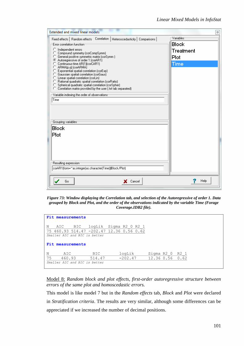
Linear Mixed Models in InfoStat
101
Figure 73: Window displaying the Correlation tab, and selection of the Autoregressive of order 1. Data
grouped by Block and Plot, and the order of the observations indicated by the variable Time (Forage
Coverage.IDB2 file).
Fit measurements
N AIC BIC logLik Sigma R2_0 R2_1
75 460.93 514.47 -202.47 12.36 0.56 0.62 Smaller AIC and BIC is better
Fit measurements
N AIC BIC logLik Sigma R2_0 R2_1
75 460.93 514.47 -202.47 12.36 0.56 0.62 Smaller AIC and BIC is better
Model 8: Random block and plot effects, first-order autoregressive structure between
errors of the same plot and homoscedastic errors.
This model is like model 7 but in the Random effects tab, Block and Plot were declared
in Stratification criteria. The results are very similar, although some differences can be
appreciated if we increased the number of decimal positions.

Linear Mixed Models in InfoStat
102
Fit measurements
N AIC BIC logLik Sigma R2_0 R2_1 R2_2
75 462.93 518.38 -202.47 12.36 0.56 0.62 0.62
Smaller AIC and BIC is better
Model 9: Random block effects, first-order autoregressive structure between errors of
the same plot and heteroscedastic errors
This model is specified as model 7. In the Heteroscedasticity tab the varIdent option is
selected, and Time declared in the Grouping variables window.
Fit measurements
N AIC BIC logLik Sigma R2_0 R2_1
75 462.70 523.89 -199.35 7.49 0.56 0.58 Smaller AIC and BIC is better
Model 10: Random block and plot effects, first-order autoregressive structure between
errors of the same plot and heteroscedastic errors
This model is specified as model 8. In the Heteroscedasticity tab the varIdent option is
selected, and Time declared in the Grouping variables window.
Fit measurements
N AIC BIC logLik Sigma R2_0 R2_1 R2_2
75 464.70 527.80 -199.35 7.49 0.56 0.58 0.58 Smaller AIC and BIC is better
Model 11: Random block effects, unstructured correlations between errors from the
same plot and time-varying residual variances.
In the Correlation tab the General positive symmetric matrix option was selected
(Figure 74) and in the Heteroscedasticity tab the varIdent option was kept (as in Figure
71). In the Random effects tab, only Block was declared in Stratification criteria (it is
not possible to fit a model including both random plot effect and general correlation at
the same grouping level. This model would be unidentifiable, and its estimates not
valid. Although the program may show an output, this is not correct).

Linear Mixed Models in InfoStat
103
Figure 74: Window displaying the Correlation tab, and the selection of the General positive symmetric
matrix Model for the data grouped by plot, and the order of the observations indicated by the variable
Time (Forage Coverage.IDB2 file).
Fit measurements
N AIC BIC logLik Sigma R2_0 R2_1
75 434.74 513.14 -176.37 6.48 0.56 0.59 Smaller AIC and BIC is better
Selection of the covariance structure
Upon comparing the values of AIC (or BIC) for the structures that we have fitted, note
that that Model 11 (AIC = 434.74, BIC = 513.14) produces the lowest value. Because of
this, we select the unstructured covariance matrix (General positive symmetric matrix).
The following are the parameters estimated by this model:
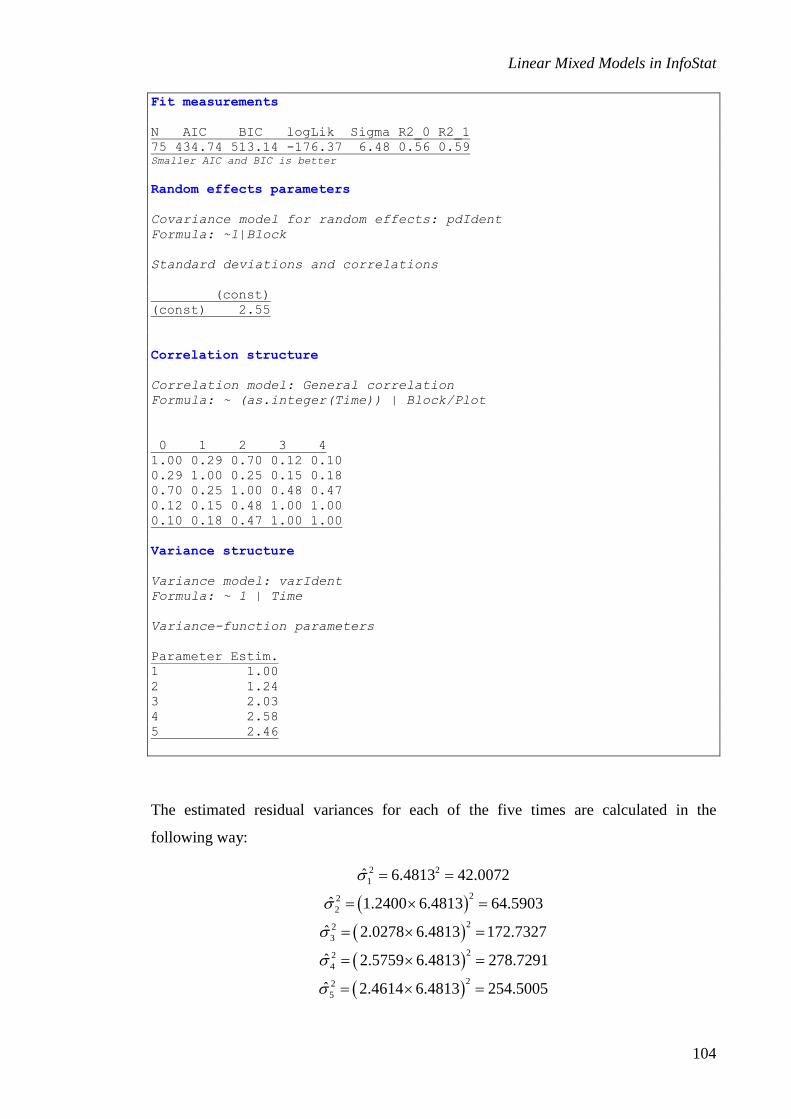
Linear Mixed Models in InfoStat
104
Fit measurements
N AIC BIC logLik Sigma R2_0 R2_1
75 434.74 513.14 -176.37 6.48 0.56 0.59 Smaller AIC and BIC is better
Random effects parameters
Covariance model for random effects: pdIdent
Formula: ~1|Block
Standard deviations and correlations
(const)
(const) 2.55
Correlation structure
Correlation model: General correlation
Formula: ~ (as.integer(Time)) | Block/Plot
0 1 2 3 4
1.00 0.29 0.70 0.12 0.10
0.29 1.00 0.25 0.15 0.18
0.70 0.25 1.00 0.48 0.47
0.12 0.15 0.48 1.00 1.00
0.10 0.18 0.47 1.00 1.00
Variance structure
Variance model: varIdent
Formula: ~ 1 | Time
Variance-function parameters
Parameter Estim.
1 1.00
2 1.24
3 2.03
4 2.58
5 2.46
The estimated residual variances for each of the five times are calculated in the
following way:
2 2
1
22
2
22
3
22
4
22
5
ˆ 6.4813 42.0072
ˆ 1.2400 6.4813 64.5903
ˆ 2.0278 6.4813 172.7327
ˆ 2.5759 6.4813 278.7291
ˆ 2.4614 6.4813 254.5005

Linear Mixed Models in InfoStat
105
The 10 estimated correlations appear directly as a matrix in the Correlation Structure.
To obtain the variance of an observation, we need to add the block variance to the
residual variance shown above:
22ˆ 0.3942 6.4813 6.5277bloque
Inference regarding the means
Once the covariance structure of the data is chosen (in this case the model with no
structure), we can proceed to make inferences about the means. The average observed
profiles for every treatment are shown in Figure 65.
In a factorial experiment such as this one, where we have a treatment factor and a time
factor, the first thing we should do is verify whether an interaction between the
treatments and time exists. To do so, we can conduct a Wald test, which in InfoStat
appears directly as Treatment:Time in the marginal tests. Another option would be to
conduct a likelihood ratio test (LRT). For this test we cannot use REML, since we are
testing models with different fixed effects, and therefore the REML estimators are not
comparable. Instead, the maximum likelihood (ML) estimator is used.
Marginal hypothesis testing (Type III SS)
numDF denDF F-value p-value
(Intercept) 1 48 82.60 <0.0001
Treatment 4 48 4.05 0.0065
Time 4 48 16.77 <0.0001
Treatment:Time 16 48 1.49 0.1417
To carry out a likelihood ratio test we can fit (with ML) two models with the same
covariance structure (in this example the model without structure) but that differ in their
fixed part: one contains the interaction term (complete model) and the other one does
not (reduced model):
Complete model:
Fit measurements
N AIC BIC logLik Sigma R2_0 R2_1
75 539.51 634.52 -228.75 5.29 0.56 0.59 Smaller AIC and BIC is better
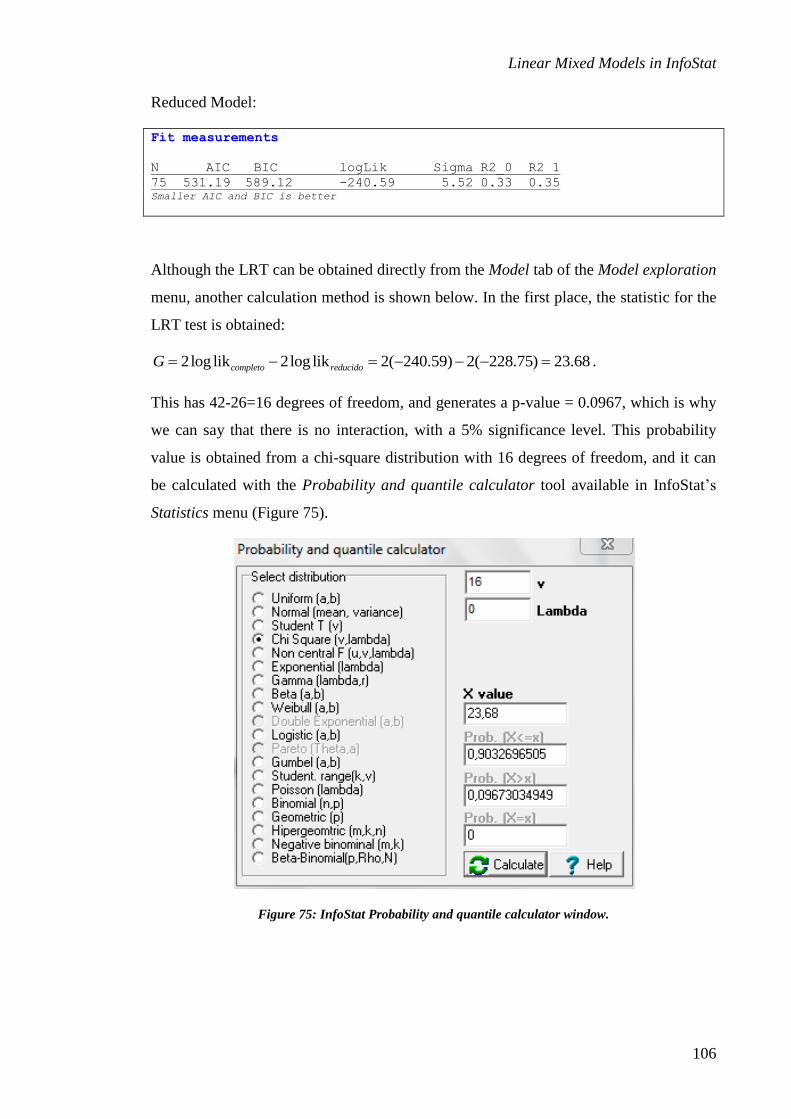
Linear Mixed Models in InfoStat
106
Reduced Model:
Fit measurements
N AIC BIC logLik Sigma R2_0 R2 1
75 531.19 589.12 -240.59 5.52 0.33 0.35 Smaller AIC and BIC is better
Although the LRT can be obtained directly from the Model tab of the Model exploration
menu, another calculation method is shown below. In the first place, the statistic for the
LRT test is obtained:
2log lik 2log lik 2( 240.59) 2( 228.75) 23.68completo reducidoG .
This has 42-26=16 degrees of freedom, and generates a p-value = 0.0967, which is why
we can say that there is no interaction, with a 5% significance level. This probability
value is obtained from a chi-square distribution with 16 degrees of freedom, and it can
be calculated with the Probability and quantile calculator tool available in InfoStat’s
Statistics menu (Figure 75).
Figure 75: InfoStat Probability and quantile calculator window.
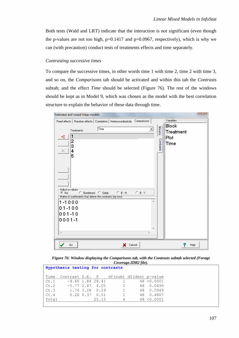
Linear Mixed Models in InfoStat
107
Both tests (Wald and LRT) indicate that the interaction is not significant (even though
the p-values are not too high, p=0.1417 and p=0.0967, respectively), which is why we
can (with precaution) conduct tests of treatments effects and time separately.
Contrasting successive times
To compare the successive times, in other words time 1 with time 2, time 2 with time 3,
and so on, the Comparisons tab should be activated and within this tab the Contrasts
subtab; and the effect Time should be selected (Figure 76). The rest of the windows
should be kept as in Model 9, which was chosen as the model with the best correlation
structure to explain the behavior of these data through time.
Figure 76: Window displaying the Comparisons tab, with the Contrasts subtab selected (Forage
Coverage.IDB2 file).
Hypothesis testing for contrasts
Time Contrast S.E. F df(num) df(den) p-value
Ct.1 -9.80 1.84 28.41 1 48 <0.0001
Ct.2 -5.77 2.87 4.05 1 48 0.0499
Ct.3 1.76 3.28 0.29 1 48 0.5949
Ct.4 0.26 0.37 0.51 1 48 0.4807
Total 25.15 4 48 <0.0001

Linear Mixed Models in InfoStat
108
The outputs shown here correspond to the REML estimations. It is clear from these
results that, on average for the four treatments, a significant change is observed between
times 1 and 2, but in subsequent times the average coverage does not change
significantly. The same conclusions are obtained by conducting a means comparison for
each time (LSD):
Adjusted means and standard error for Time
LSD Fisher (alpha=0.05)
p-value correction procedure: No
Time Means S.E.
3 30.29 3.70 A
4 28.53 4.56 A
5 28.27 4.38 A
2 24.53 2.55 A
1 14.73 2.23 B Different letters indicate significant difference between location parameters (p<= 0,05)
Comparison of treatments
Adjusted means and standard error for Treatment
LSD Fisher (alpha=0.05)
p-value correction procedure: No
Treatment Means S.E.
5 39.60 5.47 A
1 31.27 5.47 A B
4 24.96 5.47 A B C
3 17.33 5.47 B C
2 13.19 5.47 C Means with a common letter are not significantly different (p<= 0.05)
Based on this adjusted means comparison we conclude that treatments 5, 1 and 4
provide the highest coverage and are not significantly different among each other.

Linear Mixed Models in InfoStat
109
Analysis of a trial for asthma drugs
A pharmaceutical company has examined the effects of two drugs (A and B) on the
breathing capacity of asthma patients (Littell et al. 2002, 2006). Both drugs and a
placebo (P) were randomly administered to a group of patients. Each of the three
treatments had 24 patients. The basal respiratory capacity (Bas _Resp _Cap) of each
patient was measured immediately before the treatment was applied and once an hour
during the 8 hours following treatment application (Res_ Cap). The data are in the
Respiratory capacity.IDB2 file.
Using the strategy defined in the previous examples, first models with different
covariance structures will be fitted by appropriately combining residual correlation
structures, residual heteroscedasticity, and random effects. The model that best
describes the data will be selected by using penalized likelihood criteria (AIC and BIC)
and likelihood ratio tests. Once the adequate variance structure coefficient is selected,
inferences will be made about the means (compare drugs means, study the effect of
time, analyze whether the average profiles vary through time, whether they are parallel,
etc.). It is important to emphasize that all the inferences regarding the means will be
based on the model with the selected covariance structure.
Since the variable that identifies the patient (Patient) in the database takes on equal
values for each drug, in order to identify the 72 patients in this study a new variable had
to be created (Patient_drugs) that completely identifies the patient. To do so, use the
Data menu, select the Make a new column by merging categorical variables submenu
(selecting Patient and Drugs in the variables selector window). This is a two-factor
experiment, and the model used takes into account the factors Drugs, Hours and their
interaction, and the covariate Basal _Resp _Cap (all fixed effects). To conduct the
analysis for this model, the variables need to be declared in the following way (Figure
77).

Linear Mixed Models in InfoStat
110
Figure 77: Variable selector window (Respiratory capacity.IDB2 file).
First, a group of models will be evaluated to determine which one has the better fit. The
following models are evaluated:
1. Independent errors and homoscedastic residual variances.
2. Compound symmetry and homoscedastic residual variances.
3. First-order autoregressive and homoscedastic residual variances.
4. First-order autoregressive and heteroscedastic residual variances.
5. First-order autoregressive, homoscedastic residual variances, and random patient effect.
6. First-order autoregressive, heteroscedastic residual variances, and random patient effect.
7. Variances matrix and covariance without structure and heteroscedastic residual variances.
The specification of the fixed part is the same for the seven evaluated models (Figure
78). To fit Model 1, simply activate the Go button with the fixed effects model
presented below: button with fixed effects model present below:

Linear Mixed Models in InfoStat
111
Figure 78: Window displaying the Fixed effects tab (Respiratory capacity.IDB2 file).
To fit Model 2, the windows should be specified as in Figure 78 and Figure 79. Model 3
is specified as in Figure 78 and Figure 80. Model 4 is specified as in the preceding
model but including heterogenious residual variances, as shown in Figure 81. Model 5
is specified with the windows as shown in Figure 78, Figure 80 and Figure 82. Model 6
is like Model 5 but incldues the specification of the heterogeneous residual variances
(Figure 81). Model 7 is specified as shown in Figure 78, Figure 81 and Figure 83).

Linear Mixed Models in InfoStat
112
Figure 79: Window displaying the Correlation tab, with the Compound symmetry option selected
(Respiratory capacity.IDB2 file).
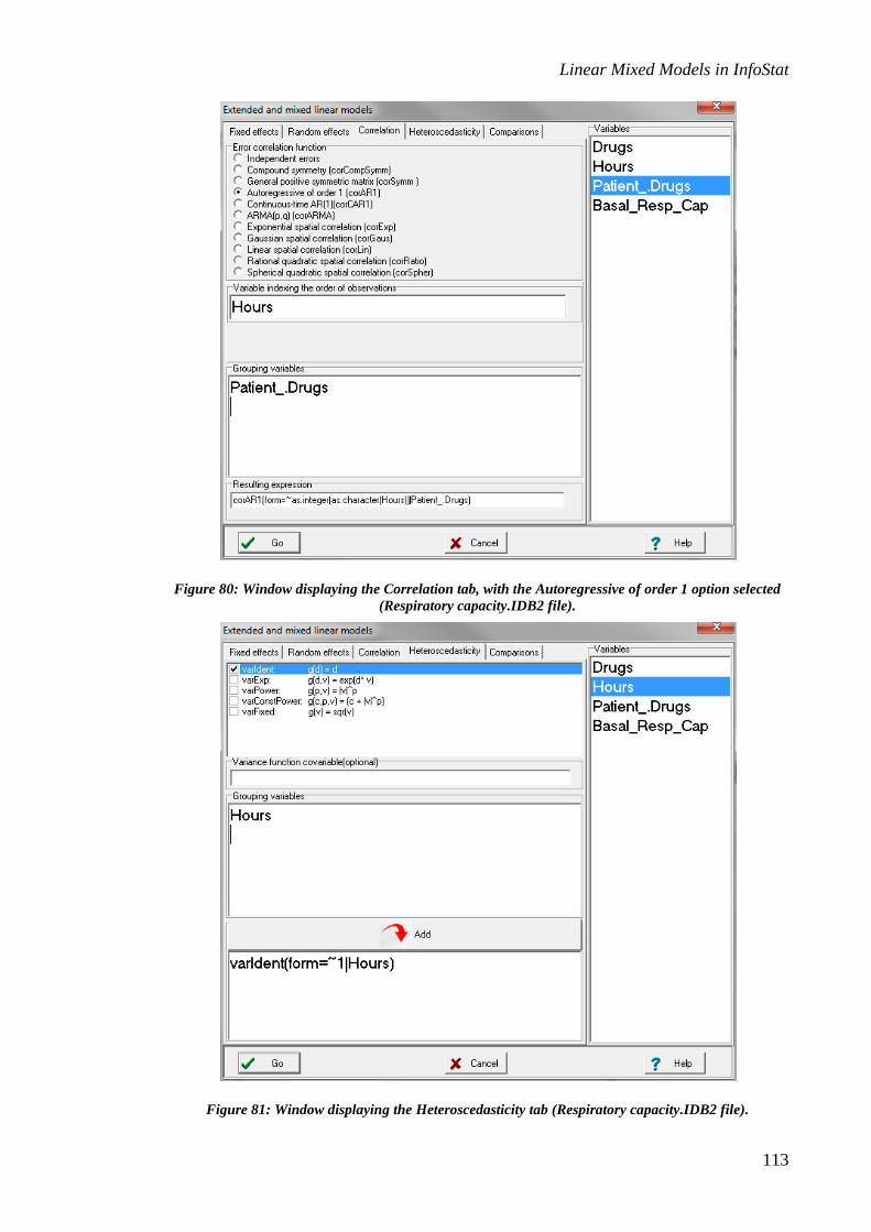
Linear Mixed Models in InfoStat
113
Figure 80: Window displaying the Correlation tab, with the Autoregressive of order 1 option selected
(Respiratory capacity.IDB2 file).
Figure 81: Window displaying the Heteroscedasticity tab (Respiratory capacity.IDB2 file).
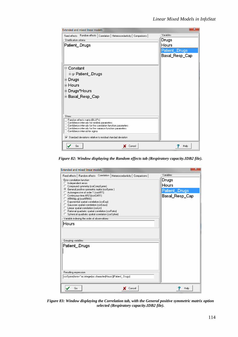
Linear Mixed Models in InfoStat
114
Figure 82: Window displaying the Random effects tab (Respiratory capacity.IDB2 file).
Figure 83: Window displaying the Correlation tab, with the General positive symmetric matrix option
selected (Respiratory capacity.IDB2 file).

Linear Mixed Models in InfoStat
115
After fitting the following models these are the results:
Table 2. Characteristics and fitted measures of the evaluated model (Respiratory
capacity.IDB2 file).
Model
Patient
random
effect
Residual
correlation
Heterogeneous
residual
variances in
Time
AIC BIC log lik
1 Yes No No 968.94 1081.04 -458.47
2 No Compound
Simmetry No 401.29 517.71 -173.65
3 No AR1 No 329.04 445.45 -137.52
4 No AR1 Yes 324.57 471.17 -128.28
5 Yes AR1 No 303.03 423.76 -123.52
6 Yes AR1 Yes 287.80 438.71 -108.90
7 No
General positive
symmetric
matrix
Yes 270.27 533.29 -74.14
From Table 2 we can observe that models 6 and 7 have the lowest AIC values, while
models 5 and 6 have the lowest BIC values. A formal likelihood ratio test used to
compare models 5 and 6 can be obtained by means of the following equation:
𝑋2 = −2(𝑙𝑜𝑔𝑙𝑖𝑛𝑘 𝑟𝑒𝑑𝑢𝑐𝑒𝑑 𝑚𝑜𝑑𝑒𝑙 − 𝑙𝑜𝑔𝑙𝑖𝑛𝑘 𝑓𝑢𝑙𝑙 𝑓𝑢𝑙𝑙 𝑚𝑜𝑑𝑒𝑙 )
= −2(−123.52 + 108.90) = 29.24
Because both models differ in 7 parameters (Model 5 has a single residual variance and
Model 6 has 8 residual variances), the likelihood ratio test statistic is compared to a
critical value of a chi-square distribution with 7 degrees of freedom. When this is done
with InfoStat’s Probabilities and quantiles calculator we obtain a p-value of 0.0001,
which leads us to choose the complete model (Model 6).
The same test can be done with the Statistics>> Extended and mixed linear models >>
Model exploration menu. To compare both models we select the Models tab and obtain
the following results:
Comparison of models
Model df AIC BIC logLik Test L.Ratio p-value
5 28 303.03 423.76 -123.52
6 35 287.80 438.71 -108.90 1 vs 2 29.23 0.0001

Linear Mixed Models in InfoStat
116
The results from the likelihood ratio test indicate that Model 6 is the better model of the
two. Now, we only need to compare Model 6 to Model 7. In this case the reduced model
is 6 and the complete model is 7. The results for this comparison are following:
Comparison of models
Model df AIC BIC logLik Test L.Ratio p-value
7 61 270.27 533.29 -74.14
6 35 287.80 438.71 -108.90 1 vs 2 69.53 <0.0001
The complete output for this model indicates that Model 7 is the best one. Therefore the
selected model has a residual correlation without structure and heterogeneous residual
variances in time. The complete output for this model is shown below:
Extended and mixed linear models
R specification of the model
model001_Res_Cap_REML<-
gls(Res_Cap~1+Drugs+Hours+Drugs:Hours+Basal_Resp_Cap
,weight=varComb(varIdent(form=~1|Hours))
,correlation=corSymm(form=~as.integer(as.character(Hours))|Patient_.Dr
ugs)
,method="REML"
,na.action=na.omit
,data=R.data00)
Results for model: model001_Res_Cap_REML
Dependent variable:Res_Cap
Fit measurements
N AIC BIC logLik Sigma R2_0
576 270.27 533.29 -74.14 0.48 0.55 Smaller AIC and BIC is better
Marginal hypothesis testing(Type III SS)
numDF F-value p-value
(Intercept) 1 6.49 0.0111
Drugs 2 7.25 0.0008
Hours 7 13.72 <0.0001
Basal_Resp_Cap 1 92.57 <0.0001
Drugs:Hours 14 4.06 <0.0001
Sequential hypothesis testing
numDF F-value p-value
(Intercept) 1 3936.01 <0.0001
Drugs 2 13.87 <0.0001
Hours 7 13.72 <0.0001
Basal_Resp_Cap 1 92.57 <0.0001
Drugs:Hours 14 4.06 <0.0001
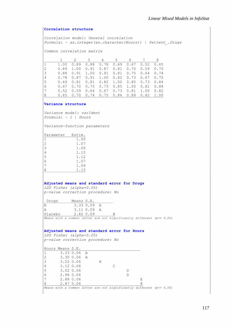
Linear Mixed Models in InfoStat
117
Correlation structure
Correlation model: General correlation
Formula: ~ as.integer(as.character(Hours)) | Patient_.Drugs
Common correlation matrix
1 2 3 4 5 6 7 8
1 1.00 0.89 0.88 0.78 0.69 0.67 0.52 0.65
2 0.89 1.00 0.91 0.87 0.81 0.70 0.59 0.70
3 0.88 0.91 1.00 0.91 0.81 0.75 0.64 0.74
4 0.78 0.87 0.91 1.00 0.82 0.73 0.67 0.75
5 0.69 0.81 0.81 0.82 1.00 0.85 0.73 0.84
6 0.67 0.70 0.75 0.73 0.85 1.00 0.81 0.88
7 0.52 0.59 0.64 0.67 0.73 0.81 1.00 0.82
8 0.65 0.70 0.74 0.75 0.84 0.88 0.82 1.00
Variance structure
Variance model: varIdent
Formula: ~ 1 | Hours
Variance-function parameters
Parameter Estim.
1 1.00
2 1.07
3 1.06
4 1.15
5 1.12
6 1.07
7 1.09
8 1.15
Adjusted means and standard error for Drugs
LSD Fisher (alpha=0.05)
p-value correction procedure: No
Drugs Means S.E.
B 3.33 0.09 A
A 3.11 0.09 A
Placebo 2.82 0.09 B Means with a common letter are not significantly different (p<= 0.05)
Adjusted means and standard error for Hours
LSD Fisher (alpha=0.05)
p-value correction procedure: No
Hours Means S.E.
1 3.33 0.06 A
2 3.30 0.06 A
3 3.22 0.06 B
4 3.12 0.06 C
5 3.02 0.06 D
6 2.96 0.06 D
7 2.88 0.06 E
8 2.87 0.06 E Means with a common letter are not significantly different (p<= 0.05)

Linear Mixed Models in InfoStat
118
Adjusted means and standard error for Drugs*Hours
LSD Fisher (alpha=0.05)
p-value correction procedure: No
Drug Hours Means S.E.
B 1 3.69 0.10 A
B 2 3.63 0.10 A B
B 3 3.58 0.10 A B
A 1 3.47 0.10 A B C
B 4 3.44 0.11 B C D
A 2 3.39 0.10 B C D
B 5 3.25 0.11 C D E
A 3 3.18 0.10 D E F
B 6 3.08 0.10 E F G
A 5 3.05 0.11 E F G H
A 4 3.04 0.11 E F G H
B 8 3.01 0.11 E F G H I
A 6 2.98 0.10 E F G H I
B 7 2.98 0.11 F G H I
P 3 2.90 0.10 F G H I
P 2 2.89 0.10 G H I
P 4 2.87 0.11 G H I
A 7 2.87 0.11 G H I
A 8 2.86 0.11 G H I
P 1 2.83 0.10 G H I
P 6 2.82 0.10 G H I
P 7 2.79 0.11 H I
P 5 2.77 0.11 H I
P 8 2.73 0.11 I Means with a common letter are not significantly different (p<= 0.05)
Note that there is a significant interaction between the drug and time (p<0.0001), so we
proceed to carry out an interaction graph. To make this graph, first the Adjusted means
and standard errors for Drugs*Hours were copied and pasted in a new InfoStat table.
This table was saved as Respiratory capacity average.IDB2. Then in the Graphs>>Dot
plot menu the variables were declared as shown below (Figure 84 and Figure 85):
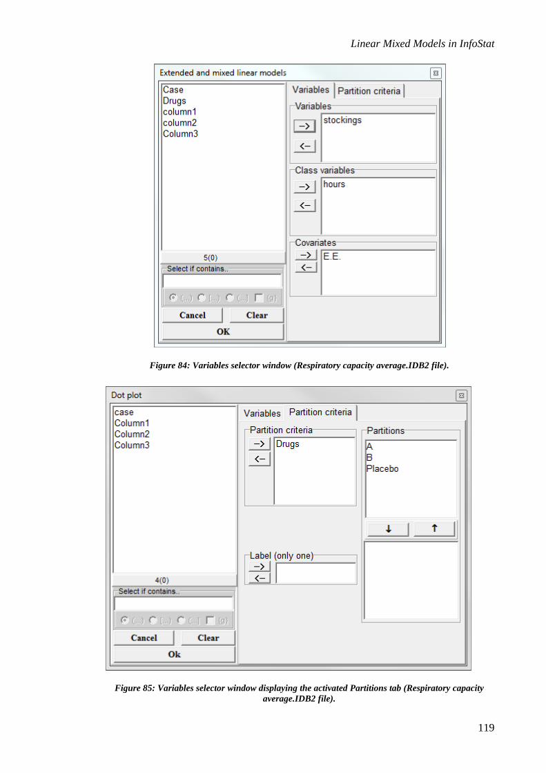
Linear Mixed Models in InfoStat
119
Figure 84: Variables selector window (Respiratory capacity average.IDB2 file).
Figure 85: Variables selector window displaying the activated Partitions tab (Respiratory capacity
average.IDB2 file).

Linear Mixed Models in InfoStat
120
It is important to emphasize that because the standard errors of each of the combinations
of treatments and hours are different, these should be taken into account when
requesting the graph. This is achieved by declaring the error measure in the Error sub-
window. With these specifications a graph is obtained to the study of the interaction
(Figure 86).
Figure 86: Box plot to study the interactions between treatments and time with the data from the
Respiratory capacity.IDB2 file.
We can observe that while the placebo has a practically constant response, drugs A and
B increase the respiratory capacity after their application. This capacity is going to
decrease with time, and the mean value of drug B is always greater than that of drug A.
In order to find significant differences between the treatments, contrasts can be
conducted within each hour. In this case, at each hour we can test hypotheses regarding
the equality of means between the drugs and the placebo, and between the two drugs.
To obtain the contrasts (in this case orthogonal) these should be declared in the
Comparisons tab, in the Contrasts subtab, as shown in Figure 87.
Drug A
Drug B
Placebo
1 2 3 4 5 6 7 8
Hours
2.6
2.7
2.8
2.9
3.0
3.1
3.2
3.3
3.4
3.5
3.6
3.7
3.8
Re
sp
ira
tory
ca
pa
city a
ve
rag
e
Drug A
Drug B
Placebo

Linear Mixed Models in InfoStat
121
Figure 87: Window displaying the Comparisons tab, Contrasts subtab (Respiratory capacity.IDB2 file).
The p-values for the requested contrasts are shown below:
hypothesis testing for contrasts
Drugs*Hours F df(num) df(den) p-value
Ct.1 40.08 1 551 <0.0001
Ct.2 2.54 1 551 0.1119
Ct.3 23.46 1 551 <0.0001
Ct.4 2.46 1 551 0.1170
Ct.5 14.55 1 551 0.0002
Ct.6 7.36 1 551 0.0069
Ct.7 7.39 1 551 0.0068
Ct.8 6.37 1 551 0.0119
Ct.9 8.11 1 551 0.0046
Ct.10 1.63 1 551 0.2022
Ct.11 2.86 1 551 0.0914
Ct.12 0.53 1 551 0.4651
Ct.13 1.09 1 551 0.2965
Ct.14 0.53 1 551 0.4656
Ct.15 2.13 1 551 0.1446
Ct.16 0.94 1 551 0.3319
Total 5.19 16 551 <0.0001

Linear Mixed Models in InfoStat
122
Contrasts 1, 3, 5, 7 and 9 compare the placebo to the average of the drugs for hours 1, 2,
3, 4 and 5 respectively. Seeing that all of these are significant (p<0.05) we can say that
at hour 6 after the drugs were administered, the drugs lose their effect, since contrasts
11, 13 and 15 are not significant. Regarding the drug comparisons among each other,
the superiority of B over A is manifested (p<0.05) only in hours 3 and 4 (contrasts 6 and
8 respectively).

Linear Mixed Models in InfoStat
123
Analysis of litter decomposition bags
In the leaf litter decomposition trials the remnant dry matter at each time is generally
analyzed through ANCOVA, using time as a covariate and a logarithmic transformation
of the response, or ANOVA for a split-plot design, when the evaluation periods are
equidistant. The experimental units consist of bags containing the vegetative material.
Usually, these bags are grouped to form a repetition that can be evaluated through time,
and the contents of each bag are evaluated at different times. Even though each time the
evaluated bags are different, often the correlation structure that assumes independence
or compound symmetry (induced by grouping of bags that represent a repetition) is not
enough to explain the observed correlations. Observations closer in time tend to be
more correlated than those distant in time, or correlations between observations from
earlier times are different from correlations between observations from later times. The
use of mixed models allows us not only to manage more complex correlation structures
but also makes it possible to model heterogeneous variances. In these models, the
treatments can be included as classification factors and time can be model as a covariate
or as a factor. This last case produces models that are less parsimonious but more
flexible in terms of their ability to model different trends through time. On the other
hand, the introduction of random effects on the parameters that involve time can be used
to correct the lack of fit.
In the example shown below, a data set generated by a decomposition trial conducted in
a tropical aquatic environment is analyzed (Martinez 2006). The compared treatments
consist of the following: two Species (Guadua sp. and Ficus sp.) of which vegetative
material is obtained, and two types of Bag in which the material is placed (Fine and
Coarse). The four treatments had 5 repetitions (with 7 bags each), and they were
evaluated at 7 times. The purpose of this trial was to establish the effect of Species, Bag
and Time on the rate of decomposition. The data can be found in the
Decomposition.IDB2 file.
The original data (remnant dry matter) were transformed to logarithms. The graph
showing the logarithm of the remnant dry matter (from here on, the response) as a
function of time and for each treatment (Figure 88) shows a decrease of the remnant dry
weight as a function of time. The graph also suggests the existence of heteroscedasticity
that is a function of time, which depends on the species and the type of bag. An initial
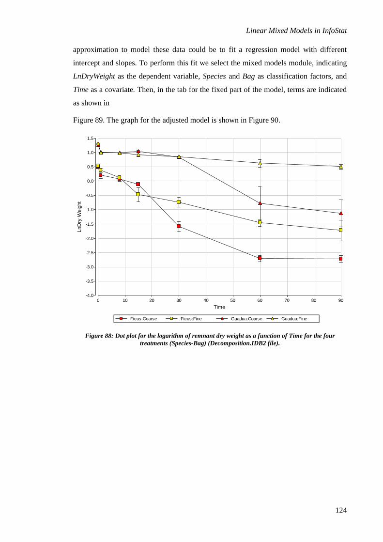
Linear Mixed Models in InfoStat
124
approximation to model these data could be to fit a regression model with different
intercept and slopes. To perform this fit we select the mixed models module, indicating
LnDryWeight as the dependent variable, Species and Bag as classification factors, and
Time as a covariate. Then, in the tab for the fixed part of the model, terms are indicated
as shown in
Figure 89. The graph for the adjusted model is shown in Figure 90.
Figure 88: Dot plot for the logarithm of remnant dry weight as a function of Time for the four
treatments (Species-Bag) (Decomposition.IDB2 file).
Ficus:Coarse Ficus:Fine Guadua:Coarse Guadua:Fine
0 10 20 30 40 50 60 70 80 90
Time
-4.0
-3.5
-3.0
-2.5
-2.0
-1.5
-1.0
-0.5
0.0
0.5
1.0
1.5
LnD
ry W
eig
ht
Ficus:Coarse Ficus:Fine Guadua:Coarse Guadua:Fine

Linear Mixed Models in InfoStat
125
Figure 89: Specification of the linear regression model with different intercepts and slopes for the
logarithm of remnant dry matter as a function of Time for the four treatments determined by the
combination of species and bag type (Species-Bag) (Decomposition.IDB2 file).
Figure 90: Dot plot for the Predicted value (logarithm of remnant dry weight) as a function of Time for
the four treatments (Species-Bag) (Decomposition.IDB2 file).

Linear Mixed Models in InfoStat
126
Figure 90 shows that the fit of different straight lines by treatment is an approximation
that, although plausible, does not account for some of the particularities of the loss of
dry weight. This is reflected by the presence of curvatures in the residuals (Figure 91).
A way to resolve the problem of the presence of curvature is the specification of a
model that includes quadratic terms for time. For this, we must extend the model
proposed in
Figure 89 to include all the terms that correspond to squared time. To simplify the
notation, we have created three variables, T1 and T2 represent time and time squared,
respectively. T1 is time centered with respect to the value 30 (days) and T2 is the square
of T1.The covariates are centered in order to eliminate the colinearity that results from
using a regressor and its square, and hence to improve the condition of the X’X matrix.
The variables T1 and T2 as well as Species_Bag are included in the
Decomposition.IDB2 file. In the specification of the mixed model, Species_Bag should
be included as a classification factor and T1 and T2 should be included as covariates.
The Fixed effects tab should look as shown in Figure 92.
Figure 91: Graph of Pearson studentized residuals vs. Time for a regression model of remnant dry
matter as a function of Time for the four treatments (Species-Bag) with different intercepts and slopes,
(Decomposition.IDB2 file).

Linear Mixed Models in InfoStat
127
Figure 92: Specification of the linear regression model with different intercepts and slopes for the
logarithm of remnant dry matter as a function of Time for the four Species-Bag treatments
(Descomposition.IDB file2).
Figure 93: Fits for the second-order polynomial regression model with different intercepts and slopes
for the logarithm of remnant dry matter as a function of Time^2 (centered) for four Species-Bag
treatments (Decomposition.IDB2 file).

Linear Mixed Models in InfoStat
128
The residuals of the fitted model according to Figure 92, show two problems:
heteroscedasticity (that depends on time and treatments) and lack of fit, seeing that for
some treatments and times, the Pearson residuals appear on top or under the zero line
(enveloped by a circle, Figure 94).
At this point, we will opt to model first the problem of heteroscedasticity using an
identity variance function. For this, we will leave the fixed part of the specification
window of the model just as indicated in Figure 92, but in the Heteroscedasticity tab we
will indicate that the variance should be estimated in a different way for the
combination of time and treatment as shown in Figure 95. Pearson’s studentized
residuals vs. time for this model are shown in Figure 96. Even if the problem of
heteroscedasticity seems mostly solved, problems of lack of fit continue to exist, and
these are visualized in groups of residuals of a single treatment in a given time that are
either all positive or all negative.
Figure 94: Studentized residuals (Pearson) vs. Time for the second-order polynomial regression model
with different intercept and slopes for the logarithm of remnant dry weight as a function of Time and
Time^2 (centered) for four Species-Bag treatments (Decomposition.IDB2 file).
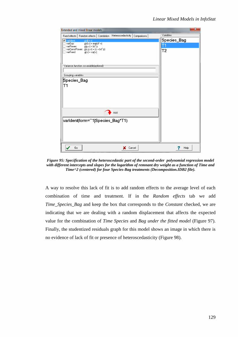
Linear Mixed Models in InfoStat
129
Figure 95: Specification of the heteroscedastic part of the second-order polynomial regression model
with different intercepts and slopes for the logarithm of remnant dry weight as a function of Time and
Time^2 (centered) for four Species-Bag treatments (Decomposition.IDB2 file).
A way to resolve this lack of fit is to add random effects to the average level of each
combination of time and treatment. If in the Random effects tab we add
Time_Species_Bag and keep the box that corresponds to the Constant checked, we are
indicating that we are dealing with a random displacement that affects the expected
value for the combination of Time Species and Bag under the fitted model (Figure 97).
Finally, the studentized residuals graph for this model shows an image in which there is
no evidence of lack of fit or presence of heteroscedasticity (Figure 98).

Linear Mixed Models in InfoStat
130
Figure 96: Studentized residuals (Pearson) vs. Time for the heteroscedastic regression model with
different intercepts and slopes by treatment for the logarithm of Remnant dry weight as a function of
Time and Time^2 (centered) for the four treatments (Species-Bag) (Decomposition.IDB2 file).
Figure 97: Specification of the random part of the second-order heteroscedastic regression model with
different intercepts and slopes for the logarithm of Remnant dry weight as a function of Time and
Time^2 (centered) for the four treatments (Species-Bag) (Decomposition.IDB2 file).

Linear Mixed Models in InfoStat
131
Figure 98: Studentized residuals (Pearson) vs. Time for the heteroscedastic regression model with
different intercept and slopes by treatment and the addition of a random effect on the constant that is
particular for each combination of Time and Treatment, for the logarithm of remnant dry weight as a
function of Time and Time^2 (centered) for the four treatments (Species-Bag) (Decomposition.IDB2
file).
Finally, since the purpose of this trial was to calculate the decomposition rate, and we
have fitted a linear model for the logarithm of the remnant dry matter weight, we can
estimate the decomposition rate as the derivative of -exp(fitted model). We will use the
interface with R to obtain these derivatives. Pressing F9 the interpreter window of R is
called (Figure 99). To the right of the window a list will appear. It contains the R
objects that have been created during the work session. In this list, the fitted models
using extended and mixed linear models should appear as a string composed of the
word “model”+ correlative number _name of the dependent variable_ Estimation
method. In our example they should appear as follows: model#_LnDryWeight _REML
(in position # there should be a number dependent on the number of times that the
model was fit for the same dependent variable). The example shows the model
modelOO1_LnDryWeight _REML.

Linear Mixed Models in InfoStat
132
Figure 99: R interface with four panels: Script contains the R programs to be executed, Output shows
the executed script, Objects shows the list of objects retained in R’s memory, and the bottom panel
shows messages and error reports sent by R to the console.
To calculate the decomposition rates, we must first understand what we have fitted with
the estimated linear model. The fixed part of the proposed model is as follows:
Species_Bag
T1
T2
Species_Bag*T1
Sspecies_Bag*T2
Este modelo es equivalente a:
Species_Bag-1
Species_Bag*T1
Species_Bag*T2
The advantage of the previous specification is that the coefficients of the fixed part of
the model correspond with those in (10). This model specifies a second-order
polynomial regression in time (centered around 30 days) for each of the combinations of
Species and Bag. Thus, we are estimating a function of the following form:

Linear Mixed Models in InfoStat
133
𝐿𝑛𝐷𝑟𝑦𝑊𝑒𝑖𝑔ℎ𝑡 = 𝛽𝑖0 + 𝛽𝑖1(𝑇 − 30) + 𝛽𝑖2(𝑇 − 30)2 (10)
where the i index indicates the treatment (in this case i identifies the four combinations
of Species and Bag). This means that we have an equation like (7) specific for each
condition. The estimated coefficients for the fixed part can be obtained during the model
estimation by checking the Fixed effects coefficients option in the Fixed effects tab.
Since we will use R to calculate the derivatives of equation (7), we will review these
coefficients from R. If we write Model004_LnDryWeight _REML$coefficients$fixed
in the Script window, and then at the end of the line press Shift Enter, the following
output will appear:
Species_BagFicus_Fine Species_BagFicus_Coarse
-0.7738921650 -1.3680878569
Species_BagGuadua_Fine Species_BagGuadua_Coarse
0.8162357629 0.7630705376
Species_BagFicus_Fine:T1 Species_BagFicus_Coarse:T1
-0.0326126598 -0.0508364778
Species_BagGuadua_Fine:T1 Species_BagGuadua_Coarse:T1
-0.0086055613 -0.0192635993
Species_BagFicus_Fine:T2 Species_BagFicus_Coarse:T2
0.0002938702 0.0004422140
Species_BagGuadua_Fine:T2 Species_BagGuadua_Coarse:T2
0.0000571603 -0.0002451274
The first four coefficients (from left to right), correspond to the constants 0i of the
following variables: Ficus_Fine, Ficus_Coarse, Guadua_Fine and Guadua_Coarse. The
Ficus_Fine constant does not appear explicitly, because it is confounded with the
intercept (Intercept), which is assumed present by default.
The second group of four coefficients (0.0326126598, ... ,-0.0192635993) are the
coefficients 1i of the linear term of (10), and the last group of four (0.0002938702,
… , -0.0002451274) are the coefficients 2i of the quadratic term in (10). The
equation for dry remnant weight for Species Ficus with Fine Bag is as follows:
2ln 0.7738921651 0.0326126598 ( 30) 0.0002938702( 30)DryWeight T T
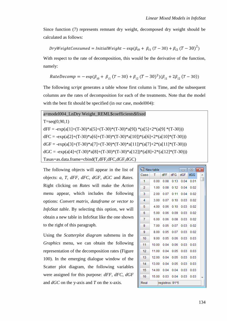
Linear Mixed Models in InfoStat
134
Since function (7) represents remnant dry weight, decomposed dry weight should be
calculated as follows:
𝐷𝑟𝑦𝑊𝑒𝑖𝑔ℎ𝑡𝐶𝑜𝑛𝑠𝑢𝑚𝑒𝑑 = 𝐼𝑛𝑖𝑡𝑖𝑎𝑙𝑊𝑒𝑖𝑔ℎ𝑡 − exp(𝛽𝑖0 + 𝛽𝑖1 (𝑇 − 30) + 𝛽𝑖2 (𝑇 − 30)2)
With respect to the rate of decomposition, this would be the derivative of the function,
namely:
𝑅𝑎𝑡𝑒𝐷𝑒𝑐𝑜𝑚𝑝 = − exp(𝛽𝑖0
+ 𝛽𝑖1
(𝑇 − 30) + 𝛽𝑖2
(𝑇 − 30)2)(𝛽𝑖1
+ 2𝛽𝑖2
(𝑇 − 30))
The following script generates a table whose first column is Time, and the subsequent
columns are the rates of decomposition for each of the treatments. Note that the model
with the best fit should be specified (in our case, model004):
a=model004_LnDry Weight_REML$coefficients$fixed
T=seq(0,90,1)
dFF = -exp(a[1]+(T-30)*a[5]+(T-30)*(T-30)*a[9]) *(a[5]+2*(a[9] *(T-30)))
dFC = -exp(a[2]+(T-30)*a[6]+(T-30)*(T-30)*a[10])*(a[6]+2*(a[10]*(T-30)))
dGF = -exp(a[3]+(T-30)*a[7]+(T-30)*(T-30)*a[11])*(a[7]+2*(a[11]*(T-30)))
dGC = -exp(a[4]+(T-30)*a[8]+(T-30)*(T-30)*a[12])*(a[8]+2*(a[12]*(T-30)))
Tasas=as.data.frame=cbind(T,dFF,dFC,dGF,dGC)
The following objects will appear in the list of
objects: a, T, dFF, dFC, dGF, dGC and Rates.
Right clicking on Rates will make the Action
menu appear, which includes the following
options: Convert matrix, dataframe or vector to
InfoStat table. By selecting this option, we will
obtain a new table in InfoStat like the one shown
to the right of this paragraph.
Using the Scatterplot diagram submenu in the
Graphics menu, we can obtain the following
representation of the decomposition rates (Figure
100). In the emerging dialogue window of the
Scatter plot diagram, the following variables
were assigned for this purpose: dFF, dFC, dGF
and dGC on the y-axis and T on the x-axis.

Linear Mixed Models in InfoStat
135
Figure 100: Decomposition curves, by species and bag type.
Ficus Fine Ficus Coarse Guadua Fino Guadua Coarse
0 10 20 30 40 50 60 70 80 90
Time
0.00
0.01
0.02
0.03
0.04
0.05
0.06
0.07
0.08
0.09
0.10
0.11
0.12
0.13
0.14
0.15
De
co
mp
ositio
n r
ate
Ficus Fine Ficus Coarse Guadua Fino Guadua Coarse

Linear Mixed Models in InfoStat
136
Use of mixed models to control spatial variability in agricultural
experiments
Spatial correlation
Stratification, or blocking, is a technique used to control the effects of variation in
experimental units. Blocks are groups of experimental units formed in such a way that
plots within blocks are as homogenous as possible. Designs with plot stratification, such
as randomized complete block designs (RCBD), incomplete block designs and lattices,
are more efficient than a completely randomized design when differences between
experimental units that make up a single stratum (block) are minimal and differences
between strata are large. When this condition is not met, the error term can be
overestimated, and if the data are unbalanced, treatment effect estimations can also be
biased. When many treatment plots are evaluated in the field, the size of the blocks
needed to obtain a repetition of the experiment is large, and consequently it is difficult
to ensure homogeneity of the plots that make up the block: plots that are closer to each
other can be more similar than plots that are farther away from each other, which
generates spatial variation (Casanoves et al. 2005). Spatial variability refers to variation
between observations obtained from plots with spatial arrangements on the field. Due to
the existence of spatial variation within blocks, standard analysis of variance for designs
that involve blocks of experimental unit does not always eliminate bias in the
comparison of treatment effects. Variation from plot to plot within a single block can be
caused by competition, heterogeneity in soil fertility, insect dispersion, weeds, crop
illness, or cultivation practices, among others. For this reason, statistical procedures that
account for spatial variation among plots and that adjust treatment means as a function
of the observations in close neighboring plots have been proposed (Papadakis 1937); as
well as models that account for spatial correlation in the error term and that also adjust
treatment means (Mead 1971, Besag 1974, 1977, Ripley 1981). Gilmour et al. (1997)
partition spatial variability among plots from an experiment in local and global spatial
variability. Local spatial variability refers to small-scale difference between plots, where
intra-block variations are considered. Local spatial trends and residual heterogeneity are
modeled with the variance and covariance residual matrix. A bi-dimensional coordinate
system allows the definition of plot location in the field. The modeling of plot spatial
structure based on distance functions can be done in the context of linear mixed models
Linear Mixed Models in InfoStat
137
(Zimmerman & Harville 1991, Gilmour et al. 1997, Cullis et al. 1998), where in
addition to accounting for the correlation structure among observations from different
plots, it is possible to model heterogeneity of residual variance. This is very useful in
comparative production experiments, since these are conducted in different
environments. If the correlation depends only on the distance (magnitude and/or
direction of the distance), models that estimate covariance among observations are
called stationary. Correlation functions for stationary models can be isotropic or
anisotropic. The former are identical in any direction (they only depend on the
magnitude of the distances) while the latter allow different parameter values in different
directions (i.e., they also depend on the direction in which the distance is calculated).
Analysis of a comparative yield trials for peanuts
To provide examples of the alternative analyses, we use data from the Peanut
MET.IDB2 file, which come from a comparative yield trial (CYT) for one agricultural
year for experimental lines (genotypes) of peanuts (Arachis hypogaea L.) from the
EEA-Manfredi, INTA, Peanut Improvement Program in Argentina. In each year, CYTs
were conducted in three locations of the cultivation area in the province of Córdoba:
Manfredi, General Cabrera and Río Tercero. The group of genotypes evaluated was the
same for each location. At each of the three locations, the experiments were conducted
according to a RCBD with four repetitions, and grain yield values were recorded
(kg/plot).
Yield data were analyzed using different modifications of the following model:
; 1,..,16; 1,..., 4; 1,...,3ijk i j k jk ik ijky i j k (11)
where ijky represents the observed response in the i-th level of the Genotype factor, in
the j-th level of the Block factor, and in the k-th level of the Location factor;
represents the general mean of the response; i represents the effect of the i-th level of
the Genotype factor; j represents the effect of the j-th level of the Block factor; k is
the k-th level of the Location factor; ik is the interaction between Genotype and
Location; ik is the effect of the Block within the Location; and ijkl represents the
experimental error. The usual assumption is that 2~ 0,ijkl N .

Linear Mixed Models in InfoStat
138
In most cases, all factors in the model are considered fixed, except for ijk and block
effects (the latter are in some cases considered random). This has the effect of
restricting the comparison of models to their own plot structure. Different plot structures
induce a correlation structure between observations that can be understood within the
framework of mixed models, including analytical techniques for the control of spatial
variability.
The following covariance structures are used for the data (marginal covariance):
1. FB Model: Fixed block effect, independent errors, constant variance between locations.
2. RB Model: Random block effect, independent errors, constant variance between locations.
3. FBE Model: Fixed block effect, independent errors, different variances between locations.
4. RBE Model: Random block effect, independent errors, different variances between locations.
5. Exp Model: Exponential spatial correlation, no block effect, constant variance between locations.
6. FBExp Model: Exponential spatial correlation, fixed block effect, constant variance between locations.
7. ExpH Model: Exponential spatial correlation, no block effect, different variances between locations.
8. Gau Model: Guassian spatial correlation, no block effect, constant variance between locations.
9. Sph Model: Spherical spatial correlation, no block effect, constant variance between locations.
In the first two models, ijk is assumed to be independent with constant variance, 2, i.e.,
the assumption is that spatial variation does not exist (intra-block) and, furthermore, that
homogeneity of residual variance exists between locations. The effects of the block are
considered fixed or random, denoted as FB Model or RB Model, respectively.
The procedures denoted as FBE Model and RBE Model are also based on a RCBD
model, but they consider possible heterogeneous residual variances depending on the
different levels of the location factor.
The fifth procedure consists in adjusting an isotropic spatial correlation model with a
correlation power function (Exp Model) for each location, without specifying a block
effect. This model assumes that an exponential function accounts for intra-block
variation as well as variation among blocks.
The sixth procedure is the same as the previous one, but with a fixed block effect
(FBExp Model).

Linear Mixed Models in InfoStat
139
The seventh model consists of a model similar to the Exp Model, but allows for the
possibility of different variances (and correlations) for each location.
The last two procedures consist in adjusting an isotropic spatial correlation model with a
function for Gaussian correlation (Gau Model) and a spherical correlation function,
without specifying a fixed block effect.
REML estimation is used in all cases. In the variables selector, Yield is indicated as a
dependent variable and Block, Location and Geno are indicated as classification
variables.
To adjust the FB Model, effects should be specified in the fixed effects tab as shown in
Figure 101.
To adjust the RB Model, factors should be specified in the fixed effects and random
effects tabs, as shown in Figure 102 andFigure 103 respectively. Nothing should be
specified in the remaining tabs.
Figure 101: Window displaying the Fixed effects tab, FB Model (Peanut MET.IDB2 file).

Linear Mixed Models in InfoStat
140
Figure 102: Window displaying the Fixed effects tab, RB Model (Peanut MET.IDB2 file).
Figure 103: Window displaying the Random effects tab, RB Model (Peanut MET.IDB2 file).
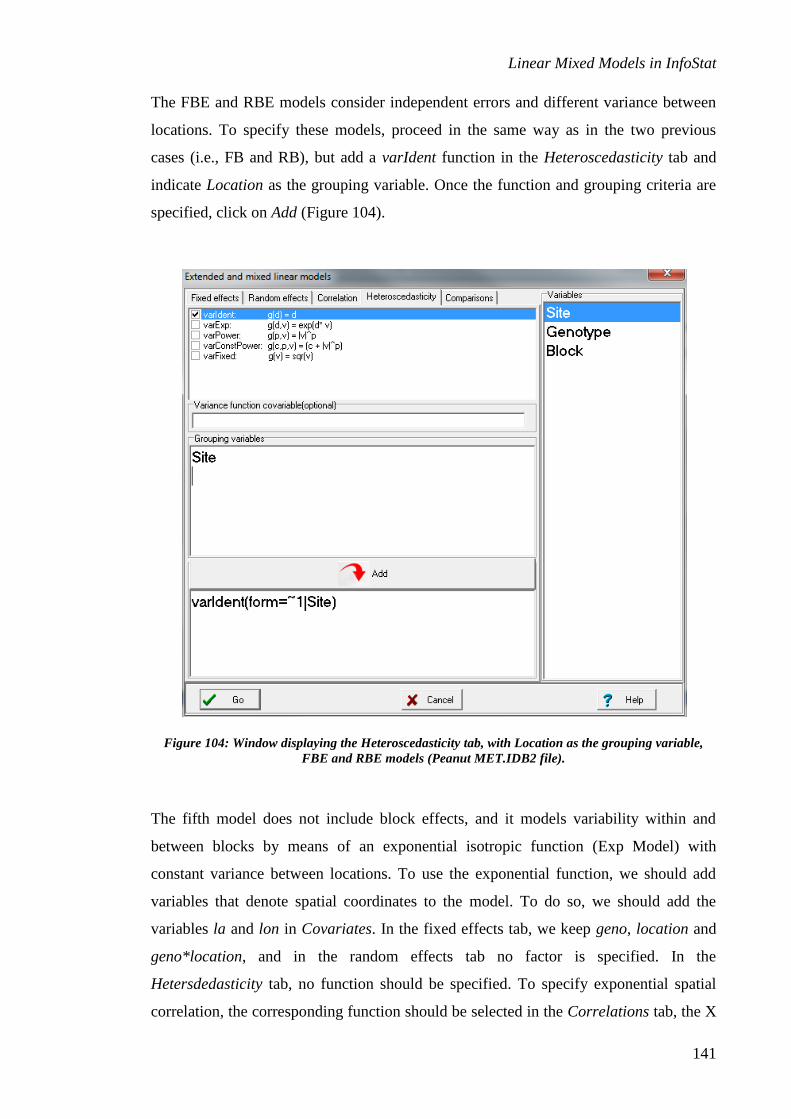
Linear Mixed Models in InfoStat
141
The FBE and RBE models consider independent errors and different variance between
locations. To specify these models, proceed in the same way as in the two previous
cases (i.e., FB and RB), but add a varIdent function in the Heteroscedasticity tab and
indicate Location as the grouping variable. Once the function and grouping criteria are
specified, click on Add (Figure 104).
Figure 104: Window displaying the Heteroscedasticity tab, with Location as the grouping variable,
FBE and RBE models (Peanut MET.IDB2 file).
The fifth model does not include block effects, and it models variability within and
between blocks by means of an exponential isotropic function (Exp Model) with
constant variance between locations. To use the exponential function, we should add
variables that denote spatial coordinates to the model. To do so, we should add the
variables la and lon in Covariates. In the fixed effects tab, we keep geno, location and
geno*location, and in the random effects tab no factor is specified. In the
Hetersdedasticity tab, no function should be specified. To specify exponential spatial
correlation, the corresponding function should be selected in the Correlations tab, the X
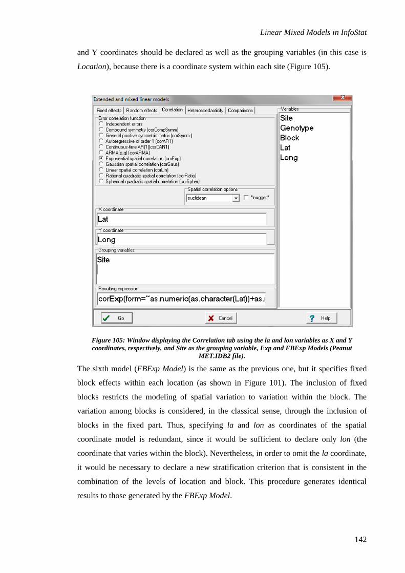
Linear Mixed Models in InfoStat
142
and Y coordinates should be declared as well as the grouping variables (in this case is
Location), because there is a coordinate system within each site (Figure 105).
Figure 105: Window displaying the Correlation tab using the la and lon variables as X and Y
coordinates, respectively, and Site as the grouping variable, Exp and FBExp Models (Peanut
MET.IDB2 file).
The sixth model (FBExp Model) is the same as the previous one, but it specifies fixed
block effects within each location (as shown in Figure 101). The inclusion of fixed
blocks restricts the modeling of spatial variation to variation within the block. The
variation among blocks is considered, in the classical sense, through the inclusion of
blocks in the fixed part. Thus, specifying la and lon as coordinates of the spatial
coordinate model is redundant, since it would be sufficient to declare only lon (the
coordinate that varies within the block). Nevertheless, in order to omit the la coordinate,
it would be necessary to declare a new stratification criterion that is consistent in the
combination of the levels of location and block. This procedure generates identical
results to those generated by the FBExp Model.
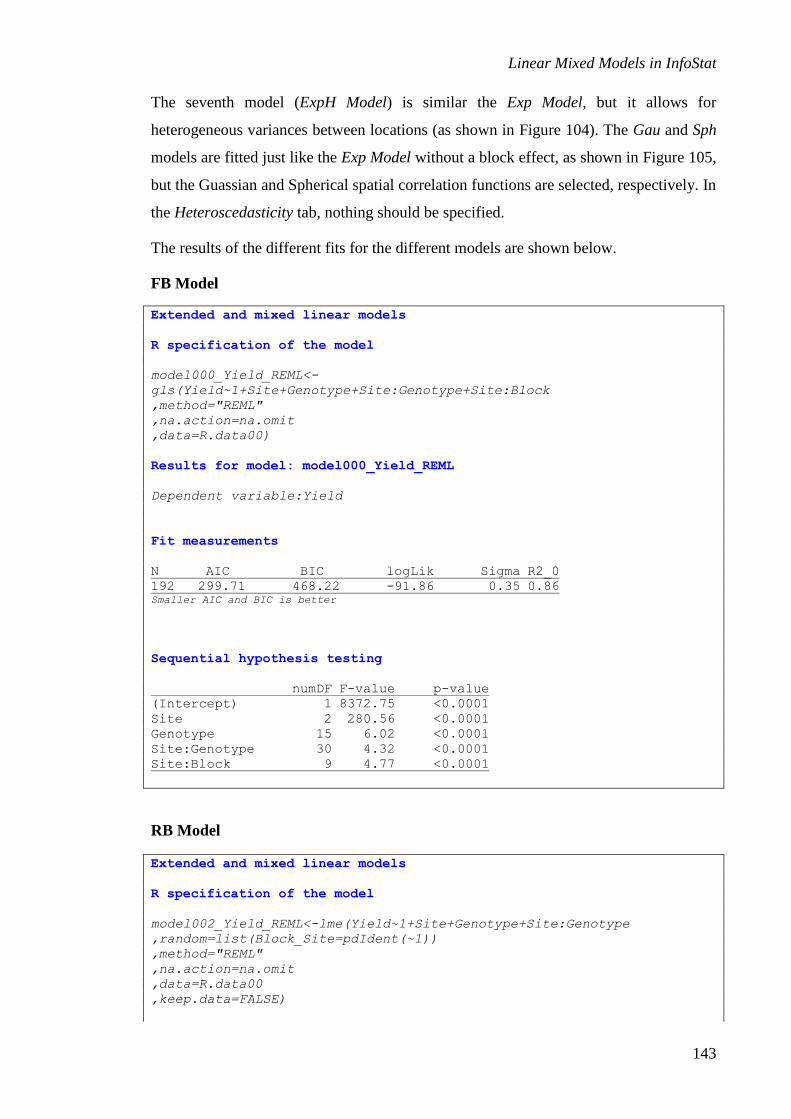
Linear Mixed Models in InfoStat
143
The seventh model (ExpH Model) is similar the Exp Model, but it allows for
heterogeneous variances between locations (as shown in Figure 104). The Gau and Sph
models are fitted just like the Exp Model without a block effect, as shown in Figure 105,
but the Guassian and Spherical spatial correlation functions are selected, respectively. In
the Heteroscedasticity tab, nothing should be specified.
The results of the different fits for the different models are shown below.
FB Model
Extended and mixed linear models
R specification of the model
model000_Yield_REML<-
gls(Yield~1+Site+Genotype+Site:Genotype+Site:Block
,method="REML"
,na.action=na.omit
,data=R.data00)
Results for model: model000_Yield_REML
Dependent variable:Yield
Fit measurements
N AIC BIC logLik Sigma R2_0
192 299.71 468.22 -91.86 0.35 0.86 Smaller AIC and BIC is better
Sequential hypothesis testing
numDF F-value p-value
(Intercept) 1 8372.75 <0.0001
Site 2 280.56 <0.0001
Genotype 15 6.02 <0.0001
Site:Genotype 30 4.32 <0.0001
Site:Block 9 4.77 <0.0001
RB Model
Extended and mixed linear models
R specification of the model
model002_Yield_REML<-lme(Yield~1+Site+Genotype+Site:Genotype
,random=list(Block_Site=pdIdent(~1))
,method="REML"
,na.action=na.omit
,data=R.data00
,keep.data=FALSE)
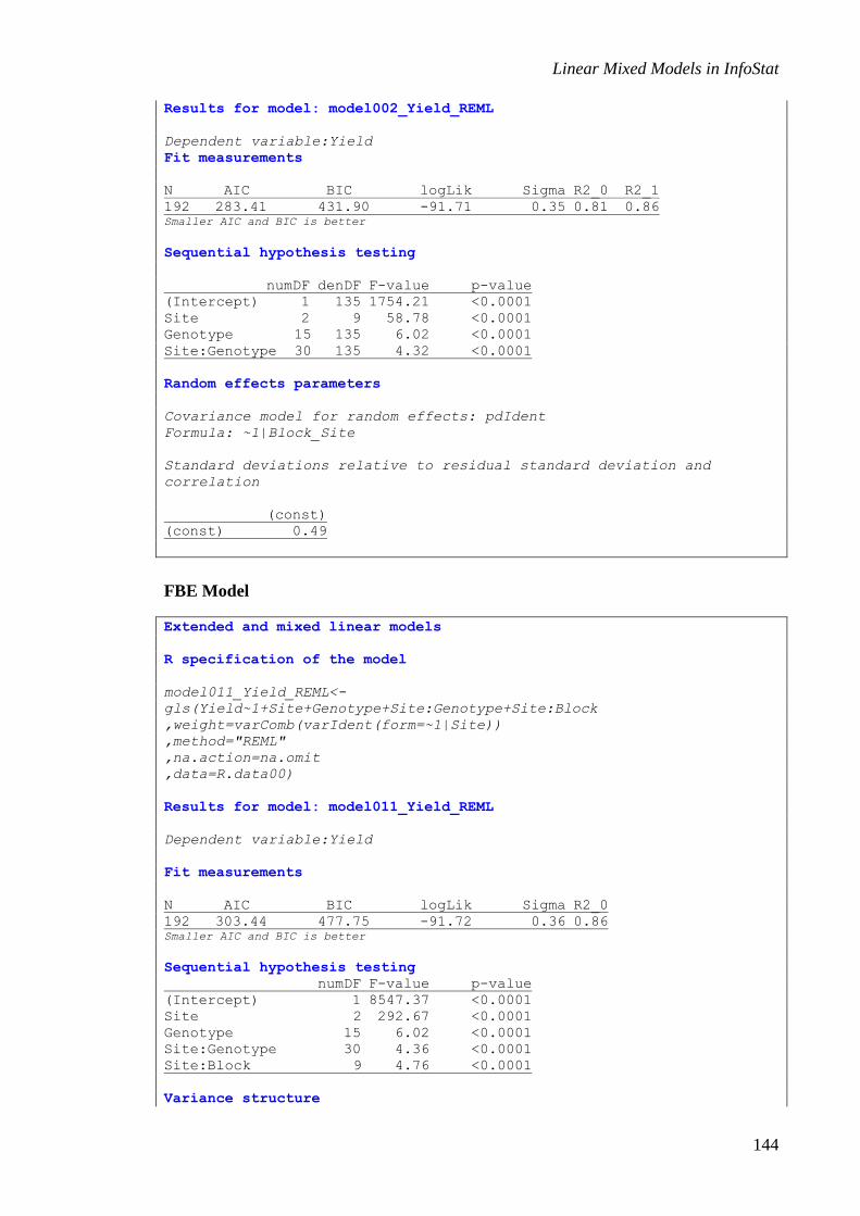
Linear Mixed Models in InfoStat
144
Results for model: model002_Yield_REML
Dependent variable:Yield
Fit measurements
N AIC BIC logLik Sigma R2_0 R2_1
192 283.41 431.90 -91.71 0.35 0.81 0.86 Smaller AIC and BIC is better
Sequential hypothesis testing
numDF denDF F-value p-value
(Intercept) 1 135 1754.21 <0.0001
Site 2 9 58.78 <0.0001
Genotype 15 135 6.02 <0.0001
Site:Genotype 30 135 4.32 <0.0001
Random effects parameters
Covariance model for random effects: pdIdent
Formula: ~1|Block_Site
Standard deviations relative to residual standard deviation and
correlation
(const)
(const) 0.49
FBE Model
Extended and mixed linear models
R specification of the model
model011_Yield_REML<-
gls(Yield~1+Site+Genotype+Site:Genotype+Site:Block
,weight=varComb(varIdent(form=~1|Site))
,method="REML"
,na.action=na.omit
,data=R.data00)
Results for model: model011_Yield_REML
Dependent variable:Yield
Fit measurements
N AIC BIC logLik Sigma R2_0
192 303.44 477.75 -91.72 0.36 0.86 Smaller AIC and BIC is better
Sequential hypothesis testing
numDF F-value p-value
(Intercept) 1 8547.37 <0.0001
Site 2 292.67 <0.0001
Genotype 15 6.02 <0.0001
Site:Genotype 30 4.36 <0.0001
Site:Block 9 4.76 <0.0001
Variance structure
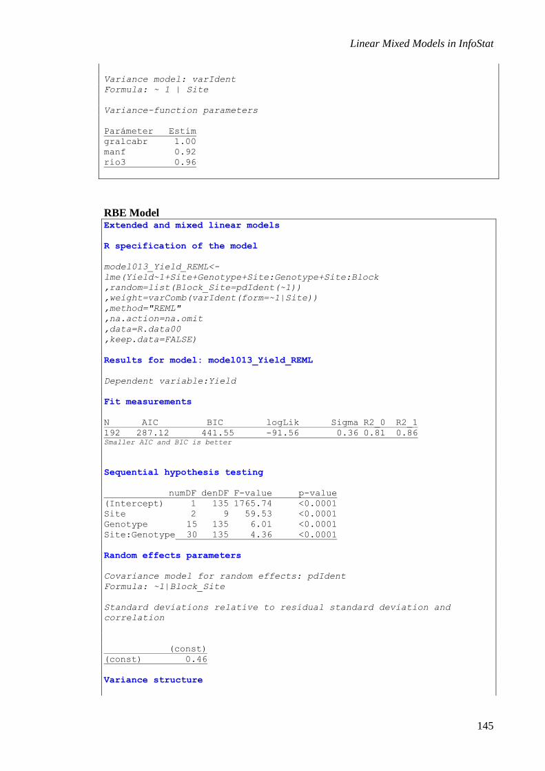
Linear Mixed Models in InfoStat
145
Variance model: varIdent
Formula: ~ 1 | Site
Variance-function parameters
Parámeter Estim
gralcabr 1.00
manf 0.92
rio3 0.96
RBE Model Extended and mixed linear models
R specification of the model
model013_Yield_REML<-
lme(Yield~1+Site+Genotype+Site:Genotype+Site:Block
,random=list(Block_Site=pdIdent(~1))
,weight=varComb(varIdent(form=~1|Site))
,method="REML"
,na.action=na.omit
,data=R.data00
,keep.data=FALSE)
Results for model: model013_Yield_REML
Dependent variable:Yield
Fit measurements
N AIC BIC logLik Sigma R2_0 R2_1
192 287.12 441.55 -91.56 0.36 0.81 0.86 Smaller AIC and BIC is better
Sequential hypothesis testing
numDF denDF F-value p-value
(Intercept) 1 135 1765.74 <0.0001
Site 2 9 59.53 <0.0001
Genotype 15 135 6.01 <0.0001
Site:Genotype 30 135 4.36 <0.0001
Random effects parameters
Covariance model for random effects: pdIdent
Formula: ~1|Block_Site
Standard deviations relative to residual standard deviation and
correlation
(const)
(const) 0.46
Variance structure

Linear Mixed Models in InfoStat
146
Variance model: varIdent
Formula: ~ 1 | Site
Variance-function parameters
Parameter Estim.
gralcabr 1.00
manf 0.92
rio3 0.95
Exp Model
Extended and mixed linear models
R specification of the model
model002_Yield_REML<-gls(Yield~1+Genotype+Site+Site:Genotype
,correlation=corExp(form=~as.numeric(as.character(Lat))+as.numeric(as.
character(Long))|Site
,metric="euclidean"
,nugget=FALSE)
,method="REML"
,na.action=na.omit
,data=R.data00)
Results for model: model002_Yield_REML
Dependent variable:Yield
Fit measurements
N AIC BIC logLik Sigma R2_0
192 273.43 421.92 -86.72 0.39 0.81 Smaller AIC and BIC is better
Sequential hypothesis testing
numDF F-value p-value
(Intercept) 1 1687.54 <0.0001
Genotype 15 7.27 <0.0001
Site 2 56.18 <0.0001
Genotype:Site 30 5.33 <0.0001
Correlation structure
Correlation model: Exponential spatial correlation
Formula: ~ as.numeric(as.character(Lat)) +
as.numeric(as.character(Long)) | Site
Metric: euclidean
Model parameters
Parameter Estim
range 0.96
FBExp Model
Extended and mixed linear models
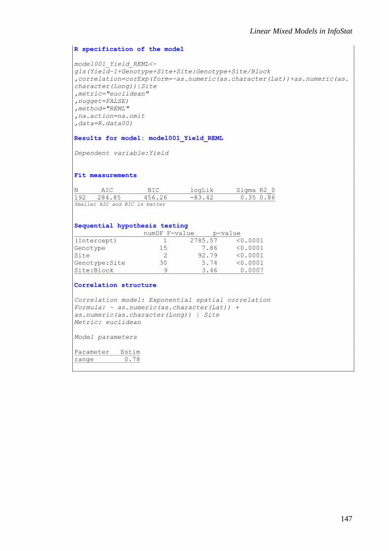
Linear Mixed Models in InfoStat
147
R specification of the model
model001_Yield_REML<-
gls(Yield~1+Genotype+Site+Site:Genotype+Site/Block
,correlation=corExp(form=~as.numeric(as.character(Lat))+as.numeric(as.
character(Long))|Site
,metric="euclidean"
,nugget=FALSE)
,method="REML"
,na.action=na.omit
,data=R.data00)
Results for model: model001_Yield_REML
Dependent variable:Yield
Fit measurements
N AIC BIC logLik Sigma R2_0
192 284.85 456.26 -83.42 0.35 0.86 Smaller AIC and BIC is better
Sequential hypothesis testing
numDF F-value p-value
(Intercept) 1 2785.57 <0.0001
Genotype 15 7.86 <0.0001
Site 2 92.79 <0.0001
Genotype:Site 30 5.74 <0.0001
Site:Block 9 3.46 0.0007
Correlation structure
Correlation model: Exponential spatial correlation
Formula: ~ as.numeric(as.character(Lat)) +
as.numeric(as.character(Long)) | Site
Metric: euclidean
Model parameters
Parameter Estim
range 0.78
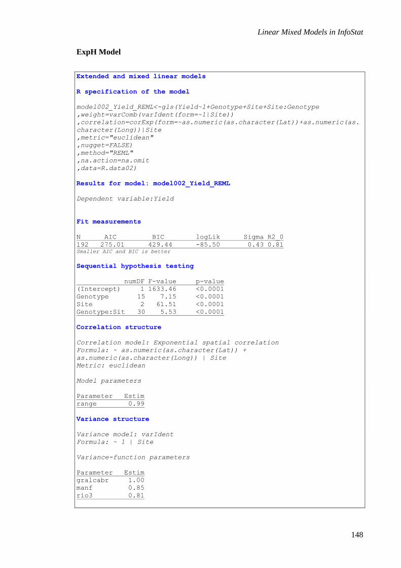
Linear Mixed Models in InfoStat
148
ExpH Model
Extended and mixed linear models
R specification of the model
model002_Yield_REML<-gls(Yield~1+Genotype+Site+Site:Genotype
,weight=varComb(varIdent(form=~1|Site))
,correlation=corExp(form=~as.numeric(as.character(Lat))+as.numeric(as.
character(Long))|Site
,metric="euclidean"
,nugget=FALSE)
,method="REML"
,na.action=na.omit
,data=R.data02)
Results for model: model002_Yield_REML
Dependent variable:Yield
Fit measurements
N AIC BIC logLik Sigma R2_0
192 275.01 429.44 -85.50 0.43 0.81 Smaller AIC and BIC is better
Sequential hypothesis testing
numDF F-value p-value
(Intercept) 1 1633.46 <0.0001
Genotype 15 7.15 <0.0001
Site 2 61.51 <0.0001
Genotype:Sit 30 5.53 <0.0001
Correlation structure
Correlation model: Exponential spatial correlation
Formula: ~ as.numeric(as.character(Lat)) +
as.numeric(as.character(Long)) | Site
Metric: euclidean
Model parameters
Parameter Estim
range 0.99
Variance structure
Variance model: varIdent
Formula: ~ 1 | Site
Variance-function parameters
Parameter Estim
gralcabr 1.00
manf 0.85
rio3 0.81

Linear Mixed Models in InfoStat
149
Gau Model
Extended and mixed linear models
R specification of the model
model004_Yield_REML<-gls(Yield~1+Genotype+Site+Site:Genotype
,correlation=corGaus(form=~as.numeric(as.character(Lat))+as.numeric(as
.character(Long))|Site
,metric="euclidean"
,nugget=FALSE)
,method="REML"
,na.action=na.omit
,data=R.data04)
Results for model: model004_Yield_REML
Dependent variable:Yield
Fit measurements
N AIC BIC logLik Sigma R2_0
192 277.81 426.30 -88.90 0.37 0.81 Smaller AIC and BIC is better
Sequential hypothesis testing
numDF F-value p-value
(Intercept) 1 3399.06 <0.0001
Genotype 15 7.36 <0.0001
Site 2 113.57 <0.0001
Genotype:Site 30 4.97 <0.0001
Correlation structure
Correlation model: Gaussian spatial correlation
Formula: ~ as.numeric(as.character(Lat)) +
as.numeric(as.character(Long)) | Site
Metric: euclidean
Model parameters
Parameter Estim
range 0.87
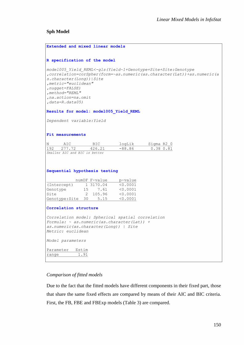
Linear Mixed Models in InfoStat
150
Sph Model
Extended and mixed linear models
R specification of the model
model005_Yield_REML<-gls(Yield~1+Genotype+Site+Site:Genotype
,correlation=corSpher(form=~as.numeric(as.character(Lat))+as.numeric(a
s.character(Long))|Site
,metric="euclidean"
,nugget=FALSE)
,method="REML"
,na.action=na.omit
,data=R.data05)
Results for model: model005_Yield_REML
Dependent variable:Yield
Fit measurements
N AIC BIC logLik Sigma R2_0
192 277.72 426.21 -88.86 0.38 0.81 Smaller AIC and BIC is better
Sequential hypothesis testing
numDF F-value p-value
(Intercept) 1 3170.04 <0.0001
Genotype 15 7.61 <0.0001
Site 2 105.96 <0.0001
Genotype:Site 30 5.15 <0.0001
Correlation structure
Correlation model: Spherical spatial correlation
Formula: ~ as.numeric(as.character(Lat)) +
as.numeric(as.character(Long)) | Site
Metric: euclidean
Model parameters
Parameter Estim
range 1.91
Comparison of fitted models
Due to the fact that the fitted models have different components in their fixed part, those
that share the same fixed effects are compared by means of their AIC and BIC criteria.
First, the FB, FBE and FBExp models (Table 3) are compared.

Linear Mixed Models in InfoStat
151
Table 3. Goodness of fit criteria for the adjusted models with a fixed block effect
(Peanut MET.IDB2 file).
Model AIC BIC
FB 299.72 468.22
FBE 303.44 477.75
FBExp 284.85 456.26
For this group of models that consider the fixed block effect, we can observe that the
fixed block model plus an exponential correlation function provides the best fit. This
implies that intra-block correlation exists, and it is removed by the exponential
correlation function. Note also that there is no improvement in the models when
heterogeneous variances between locations are allowed (FB with respect to FBE). If the
variances are calculated from the coefficients of the different locations, we can also
observe that these are very similar:
Variance of gralcabr = (1*0.36)2 = 0.129
Variance of manf = (0.92*0.36)2 = 0.109
Variance of rio3 = (0.96*0.36)2 = 0.119
The remaining 6 models can be compared among each other, given that they all share
the same fixed effects, i.e., Geno, Location and Geno*Location (Table 4).
Table 4. Goodness of fit criteria for the adjusted models without a fixed block effect
(Peanut MET.IDB2 file).
Model AIC BIC
RB 283.41 431.90
RBE 287.12 441.55
Exp 273.43 421.92
ExpH 275.01 429.44
Gau 277.81 426.30

Linear Mixed Models in InfoStat
152
Sph 277.72 426.21
Among the models that consider random block effects, we can observe that allowing for
heterogenous variances between locations does not improve the model, since AIC and
BIC are smaller in RB than in RBE. The same occurs when spatial variability is modeled
only through an exponential correlation function, because allowing for heterogeneous
variances (ExpH) does not improve the Exp Model.
Compared to different spatial correlation models, no important differences were found
for AIC and BIC between the Gau and Sph models, however these criteria had lower
values for the exponential spatial correlation function. This last model had the best fit
among the models without a fixed block effect.
Even if the first group of models (FB, FBH and FBExp) are not comparable through
AIC and BIC with this last group, the researcher should be able to determine if the
blocks should be considered fixed or random. The selection of the model group will
have an effect on the inferences that can be made. This is easily visualized by observing
that the standard errors used for the comparison of means change depending on the
model. A more detailed discussion on the selection of fixed or random blocks is
provided by Casanoves et al. (2007).
In this example, the best models within each group (i.e., FBExp and Exp for the first and
second group of models, respectively) have the same covariance structure but differ in
their fixed part: some have a block effect and others do not. In order to decide which of
the two models is best, a likelihood ratio test using ML estimations for the models with
and without block effect should be conducted (remember that ML should be used to
compare models with different fixed effects).
Model with blocks (complete FBExp):
Fit measurements
N AIC BIC logLik Sigma R2_0
192 163.82 356.01 -22.91 0.29 0.86 Smaller AIC and BIC is better
Model without blocks (reduced Exp):
Fit measurements
N AIC BIC logLik Sigma R2_0
192 182.85 345.73 -41.43 0.34 0.81 Smaller AIC and BIC is better

Linear Mixed Models in InfoStat
153
Thus, the statistic 2log lik 2log lik 2( 22.91 41.43) 37.04completo reducidoG with 9
degrees of freedom and a p-value < 0.0001. Thus we can say with a 5% confidence
level that it is best to keep the fixed block effect and the exponential correlation
function. The comparison can be done manually, or by using the module for
Exploratory analysis of an estimated model. The following result is obtained by
selecting the Models tab and checking the estimated models that correspond to FBExp
and Exp.
Comparison of models
Model df logLik Test L.Ratio p-value
model009_rendim_ML 1 59 -22.91
model010_rendim_ML 2 50 -41.43 1 vs 2 37.04 <0.0001
The complete result corresponding to the FBExp Model is shown below. The hypothesis
tests for the interaction between Genotype and Location are significant (p<0.0001), thus
the recommended Genotype can change depending on location. Note that due to the fit
of the the spatial correlation function, the standard errors of the Genotypes are not
constant. The multiple comparisons shown are generated through the application of the
DGC procedure (Di Rienzo et al. 2002). This procedure was adapted to account for the
particularities of the correlation structure among estimates in mixed models. The
application of this procedure is recommended because of the large number of means to
be compared, since it ensures a simpler interpretation than that which can be given by
an LSD or Fisher’s test. One can use the means of the combinations of locations and
Genotypes as well as the interaction graph (Figure 106) to make recommendations.
Extended and mixed linear models
R specification of the model
model007_Yield_REML<-
gls(Yield~1+Genotype+Site+Site:Genotype+Site/Block
,correlation=corExp(form=~as.numeric(as.character(Lat))+as.numeric(as.
character(Long))|Site
,metric="euclidean"
,nugget=FALSE)
,method="REML"
,na.action=na.omit
,data=R.data07

Linear Mixed Models in InfoStat
154
Results for model: model007_Yield_REML
Dependent variable:Yield
Fit measurements
N AIC BIC logLik Sigma R2_0
192 284.85 456.26 -83.42 0.35 0.86 Smaller AIC and BIC is better
Sequential hypothesis testing
numDF F-value p-value
(Intercept) 1 2785.57 <0.0001
Site 2 92.79 <0.0001
Genotype 15 7.86 <0.0001
Site:Genotype 30 5.74 <0.0001
Site:Block 9 3.46 0.0007
Correlation structure
Correlation model: Exponential spatial correlation
Formula: ~ as.numeric(as.character(Lat)) +
as.numeric(as.character(Long)) | Site
Metric: euclidean
Model parameters
Parameter Estim
range 0.78
Adjusted means and standard error for Site
DGC (alpha=0.05)
Site Means E.E.
manf 3.00 0.08 A
gralcabr 2.27 0.08 B
rio3 1.56 0.08 C Different letters indicate significant difference between location parameters (p<= 0,05)
Adjusted means and standard error for Genotype
DGC (alpha=0.05)
Genotype Means S.E.
mf435 2.73 0.10 A
mf407 2.59 0.10 A
mf429 2.51 0.10 A
mf415 2.49 0.10 A
mf420 2.38 0.10 B
mf421 2.36 0.10 B
mf431 2.34 0.10 B
mf405 2.31 0.10 B
manf68 2.24 0.10 B
mf408 2.22 0.10 B
manf393 2.22 0.10 B
colirrad 2.21 0.10 B
mf404 2.14 0.10 B
mf433 1.96 0.10 C
mf432 1.96 0.10 C
mf410 1.78 0.10 C Different letters indicate significant difference between location parameters (p<= 0,05)
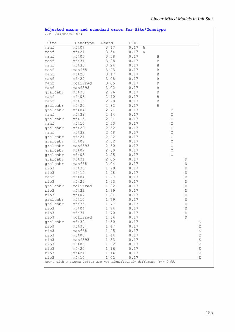
Linear Mixed Models in InfoStat
155
Adjusted means and standard error for Site*Genotype
DGC (alpha=0.05)
Site Genotype Means E.E.
manf mf407 3.67 0.17 A
manf mf421 3.54 0.17 A
manf mf405 3.38 0.17 B
manf mf431 3.28 0.17 B
manf mf435 3.24 0.17 B
manf manf68 3.23 0.17 B
manf mf420 3.17 0.17 B
manf mf429 3.08 0.17 B
manf colirrad 3.05 0.17 B
manf manf393 3.02 0.17 B
gralcabr mf435 2.96 0.17 B
manf mf408 2.90 0.17 B
manf mf415 2.90 0.17 B
gralcabr mf420 2.82 0.17 B
gralcabr mf404 2.71 0.17 C
manf mf433 2.64 0.17 C
gralcabr mf415 2.61 0.17 C
manf mf410 2.53 0.17 C
gralcabr mf429 2.52 0.17 C
manf mf432 2.48 0.17 C
gralcabr mf421 2.42 0.17 C
gralcabr mf408 2.32 0.17 C
gralcabr manf393 2.30 0.17 C
gralcabr mf407 2.30 0.17 C
gralcabr mf405 2.25 0.17 C
gralcabr mf431 2.05 0.17 D
gralcabr manf68 2.04 0.17 D
rio3 mf435 1.99 0.17 D
rio3 mf415 1.98 0.17 D
manf mf404 1.97 0.17 D
rio3 mf429 1.93 0.17 D
gralcabr colirrad 1.92 0.17 D
rio3 mf432 1.89 0.17 D
rio3 mf407 1.81 0.17 D
gralcabr mf410 1.79 0.17 D
gralcabr mf433 1.77 0.17 D
rio3 mf404 1.74 0.17 D
rio3 mf431 1.70 0.17 D
rio3 colirrad 1.64 0.17 D
gralcabr mf432 1.50 0.17 E
rio3 mf433 1.47 0.17 E
rio3 manf68 1.45 0.17 E
rio3 mf408 1.44 0.17 E
rio3 manf393 1.33 0.17 E
rio3 mf405 1.32 0.17 E
rio3 mf420 1.16 0.17 E
rio3 mf421 1.14 0.17 E
rio3 mf410 1.02 0.17 E Means with a common letter are not significantly different (p<= 0.05)

Linear Mixed Models in InfoStat
156
Figure 106: Dot plot used to study the interaction between Location and Genotype for the variable
Yield (Peanut MET.IDB).
General Cabrera Manfredi Río Tercero
mf4
04
mf4
32
mf4
10
mf4
33
mf4
15
manf3
93
mf4
08
mf4
29
colir
rad
mf4
20
mf4
31
manf6
8
mf4
35
mf4
05
mf4
21
mf4
07
Genotype
0
1
2
3
4
Yie
ld (
kg/p
lot)
General Cabrera Manfredi Río Tercero

Applications of mixed models to other experimental designs
Strip-plot design
The strip-plot design is the result of restrictions in the randomization. Like the split-plot
design, the strip-plot design results from an experiment that involves two or more
factors. These factors (or their combinations) are applied to different levels, usually 2,
and the randomization restrictions produce experimental units of different sizes and thus
produce different error terms for each of the factors or combinations thereof (Milliken
and Johnson 1992).
Consider an example in which we wish to evaluate three levels of fertilization with N
(0, 50 and 100 kg N/ha) and two irrigation levels (low and high) on corn yields (data in
Strip-plot.IDB2). The experiment was conducted under a randomized complete block
design with four blocks.
Due to restrictions in the application of treatments, in the first stage, the three levels of
nitrogen are randomized within each block; in the second stage, the irrigation levels are
randomized, within each block and transversely with respect to the application of
nitrogen.
Although in the following diagram (Figure 107) the randomization is shown within a
specific block, the experiment was repeated in various blocks, as needed in order to
obtain different error terms and for the resulting model to make sense. If each stage of
the design has more than one factor, and these do interact with each other, one could use
the interactions of highest order as error terms and thus obtain F tests without the need
for repetitions.

Linear Mixed Models in InfoStat
158
Stage 1
100 kg N/ha
0 kg N/ha
50 kg N/ha
Stage 2
High irrigation Low irrigation
Figure 107: Outline of an experiment conducted under a strip-plot design, repeated in completely
randomized blocks with the randomization of the factors Nitrogen and Amount of irrigation for a
particular block (StripPlot.IDB2 file).
Yield data were analyzed using the following model:
; 1,..,3; 1,2; 1,..., 4ijk i j ij k ki kj kijy b f c e i j k (12)
where ijky is the observed response in the i-th level of the nitrogen factor, the j-th level
of the irrigation factor, and the k-th level of the block factor; is the general mean of
the response; i is the effect of the i-th level of the nitrogen factor; j is the effect of
the j-th level of the irrigation factor; kb is the k-th level of the random Block factor; ikf
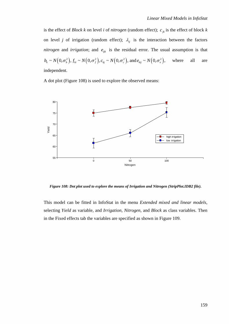
Linear Mixed Models in InfoStat
159
is the effect of Block k on level i of nitrogen (random effect); jkc is the effect of block k
on level j of irrigation (random effect); ij is the interaction between the factors
nitrogen and irrigation; and ijke is the residual error. The usual assumption is that
2 2 2 2~ 0, , ~ 0, , ~ 0, , and ~ 0,k b ki f kj c kij eb N f N c N e N , where all are
independent.
A dot plot (Figure 108) is used to explore the observed means:
Figure 108: Dot plot used to explore the means of Irrigation and Nitrogen (StripPlot.IDB2 file).
This model can be fitted in InfoStat in the menu Extended mixed and linear models,
selecting Yield as variable, and Irrigation, Nitrogen, and Block as class variables. Then
in the Fixed effects tab the variables are specified as shown in Figure 109.
high irrigation
low irrigation
0 50 100
Nitrogen
55
60
65
70
75
80
Yie
ld
high irrigation
low irrigation

Linear Mixed Models in InfoStat
160
Figure 109: Window displaying the Fixed effects tab to evaluate a mixed model (StripPlot.IDB2 file).
In the Random effects tab, the block effect should be specified for the constant ( kb ) as
well as for the fixed factors Nitrogen and Irrigation ( ikf y jkc , respectively) (Figure
110).

Linear Mixed Models in InfoStat
161
Figure 110: Window displaying the Random effects tab for mixed model (StripPlot.IDB2 file).
Extended and mixed linear models
R specification of the model
model000_Yield_REML<-
lme(Yield~1+Nitrogen+Irrigation+Nitrogen:Irrigation
,random=list(Block=pdIdent(~1)
,Block=pdIdent(~Nitrogen-1)
,Block=pdIdent(~Irrigation-1))
,method="REML"
,na.action=na.omit
,data=R.data00
,keep.data=FALSE)
Results for model: model000_Yield_REML
Dependent variable:Yield
Fit measurements
N AIC BIC logLik Sigma R2_0 R2_1 R2_2 R2_3
24 106.09 115.00 -43.05 1.20 0.85 0.94 0.95 0.99 Smaller AIC and BIC is better

Linear Mixed Models in InfoStat
162
Sequential hypothesis testing
numDF denDF F-value p-value
(Intercept) 1 15 3061.88 <0.0001
Nitrogen 2 15 60.13 <0.0001
Irrigation 1 15 52.18 <0.0001
Nitrogen:Irrigation 2 15 33.12 <0.0001
Random effects parameters
Covariance model for random effects: pdIdent
Formula: ~1|Block
Standard deviations relative to residual standard deviation and
correlation
(const)
(const) 1.83
Covariance model for random effects: pdIdent
Formula: ~Nitrogen - 1|Block
Standard deviations relative to residual standard deviation and
correlation
0 100 50
0 0.70 0.00 0.00
100 0.00 0.70 0.00
50 0.00 0.00 0.70
Covariance model for random effects: pdIdent
Formula: ~Irrigation - 1|Block
Standard deviations relative to residual standard deviation and
correlation
high low
high 1.49 0.00
low 0.00 1.49
Adjusted means and standard error for Nitrogen
LSD Fisher (alpha=0.05)
p-value correction procedure: No
Nitrogen Means S.E.
100 77.38 1.40 A
50 71.75 1.40 B
0 68.25 1.40 C Means with a common letter are not significantly different (p<= 0.05)
Adjusted means and standard error for Irrigation
LSD Fisher (alpha=0.05)
p-value correction procedure: No
Irrigation Means S.E.
high 77.33 1.47 A
low 67.58 1.47 B Means with a common letter are not significantly different (p<= 0.05)

Linear Mixed Models in InfoStat
163
Adjusted means and standard error for Nitrogen*Irrigation
LSD Fisher (alpha=0.05)
p-value correction procedure: No
Nitrogen Irrigation Means S.E.
100 high 79.50 1.59 A
50 high 77.50 1.59 A B
100 low 75.25 1.59 B C
0 high 75.00 1.59 C
50 low 66.00 1.59 D
0 low 61.50 1.59 E Means with a common letter are not significantly different (p<= 0.05)
An alternative equivalent formulation of this model is presented in Figure 111.
Figure 111: Window displaying the Random effects tab to evaluate a mixed model with Nitrogen and
Irrigation as cross factors (StripPlot.IDB2 file).

Linear Mixed Models in InfoStat
164
Extended and mixed linear models
R specification of the model
model.019_Yield_REML<-
lme(Yield~1+Nitrogen+Irrigation+Nitrogen:Irrigation
,random=list(Block=pdIdent(~1)
,Block=pdBlocked(list(pdIdent(~1)
,pdIdent(~Nitrogen-1)
,pdIdent(~Irrigation-1))))
,method="REML"
,control=lmeControl(msMaxIter=200)
,na.action=na.omit
,data=R.data19
,keep.data=FALSE)
Results for model: model.019_Yield_REML
Dependent variable: Yield
Fit measurements
N AIC BIC logLik Sigma R2_0 R2_1 R2_2
24 108.09 117.89 -43.05 1.20 0.85 0.91 0.99 Smaller AIC and BIC is better
Marginal hypothesis testing (Type III SS)
numDF denDF F-value p-value
(Intercept) 1 15 3061.88 <0.0001
Nitrogen 2 15 60.13 <0.0001
Irrigation 1 15 52.18 <0.0001
Nitrogen:Irrigation 2 15 33.12 <0.0001
Sequential hypothesis testing
numDF denDF F-value p-value
(Intercept) 1 15 3061.88 <0.0001
Nitrogen 2 15 60.13 <0.0001
Irrigation 1 15 52.18 <0.0001
Nitrogen:Irrigation 2 15 33.12 <0.0001
Random effects parameters
Covariance model for random effects: pdIdent
Formula: ~1|Block
Standard deviations and correlations
(const)
(const) 1.67
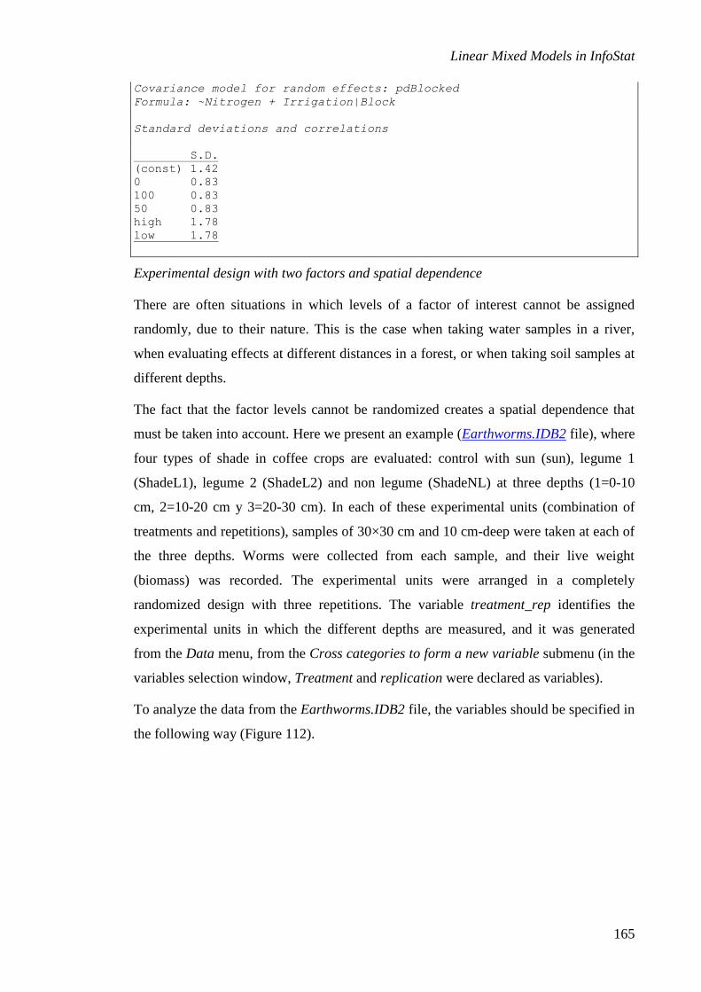
Linear Mixed Models in InfoStat
165
Covariance model for random effects: pdBlocked
Formula: ~Nitrogen + Irrigation|Block
Standard deviations and correlations
S.D.
(const) 1.42
0 0.83
100 0.83
50 0.83
high 1.78
low 1.78
Experimental design with two factors and spatial dependence
There are often situations in which levels of a factor of interest cannot be assigned
randomly, due to their nature. This is the case when taking water samples in a river,
when evaluating effects at different distances in a forest, or when taking soil samples at
different depths.
The fact that the factor levels cannot be randomized creates a spatial dependence that
must be taken into account. Here we present an example (Earthworms.IDB2 file), where
four types of shade in coffee crops are evaluated: control with sun (sun), legume 1
(ShadeL1), legume 2 (ShadeL2) and non legume (ShadeNL) at three depths (1=0-10
cm, 2=10-20 cm y 3=20-30 cm). In each of these experimental units (combination of
treatments and repetitions), samples of 30×30 cm and 10 cm-deep were taken at each of
the three depths. Worms were collected from each sample, and their live weight
(biomass) was recorded. The experimental units were arranged in a completely
randomized design with three repetitions. The variable treatment_rep identifies the
experimental units in which the different depths are measured, and it was generated
from the Data menu, from the Cross categories to form a new variable submenu (in the
variables selection window, Treatment and replication were declared as variables).
To analyze the data from the Earthworms.IDB2 file, the variables should be specified in
the following way (Figure 112).

Linear Mixed Models in InfoStat
166
Figure 112: Variables selector window for the Extended and mixed linear model (Earthworms.IDB2
file).
Then, in the Fixed effects tab, the variables should be specified as shown in the
following figure (Figure 113).

Linear Mixed Models in InfoStat
167
Figure 113: Window displaying the Fixed effects tab for evaluating a mixed model (Earthworms.IDB2
file).
Finally, the exponential spatial correlation model should be specified in the Correlation
tab; depth should be identified as the X coordinate and Treatment_rep as the grouping
variable (Figure 114).

Linear Mixed Models in InfoStat
168
Figure 114: Window displaying the Correlation tab for evaluating a mixed model with exponential
spatial correlation (Earthworms.IDB2 file).
The corresponding result is shown below.
Extended and mixed linear models
R specification of the model
model001_Biomass_REML<-gls(Biomass~1+Treatment+Depth+Treatment:Depth
,correlation=corExp(form=~as.numeric(as.character(Depth))|Treatment_Re
p
,metric="euclidean"
,nugget=FALSE)
,method="REML"
,na.action=na.omit
,data=R.data01)
Results for model: model001_Biomass_REML
Dependent variable:Biomass
Fit measurements
N AIC BIC logLik Sigma R2_0
36 161.03 177.52 -66.52 3.46 0.97 Smaller AIC and BIC is better

Linear Mixed Models in InfoStat
169
Sequential hypothesis testing
numDF F-value p-value
(Intercept) 1 3725.04 <0.0001
Treatment 3 66.75 <0.0001
Depth 2 303.14 <0.0001
Treatment:Depth 6 4.86 0.0022
Correlation structure
Correlation model: Exponential spatial correlation
Formula: ~ as.numeric(as.character(Depth)) | Treatment_Rep
Metric: euclidean
Model parameters
Parameter Estim.
range 2.12
All the resulting factors are significant, and there is an interaction between Treatment
and Depth (p=0.0022). The range parameter has an estimated value of 2.12. This
parameter should be interpreted with care, depending on the spatial correlation model
that is used. In the geostatistical bibliography, Range, for second-order stationary spatial
processes, is defined as the distance at which observations can be considered
independent. The Range parameter shown in the results is related to this definition, but
it is not the distance at which there is no more correlation (except for the spherical and
linear models). In the spatial correlation models for which the covariance only
asymptotically reaches zero (all except for spherical and linear), there is no distance at
which spatial correlation equals zero; thus, the concept is of a practical range (distance
at which covariance is reduced to 5%, or, equivalently, the distance at which the
semivariogram reaches 95% of its maximum). This distance depends on the model used:
for exponential spatial correlation it is equal to 3 times the estimated range; for the
Gaussian spatial correlation it equals √3 times the estimated range (Littel et al. 2006).
In this example, an exponential spatial correlation model is used. Depth 1 is between 0
and 10 cm, Depth 2 is between 10 and 20 cm, and Depth 3 is between 20 and 30 cm; in
other words, according to the way in which they were declared, the difference between
depths 1 and 2 is 1, however in the original scale, this difference equals 10. Thus, the
practical range of the original scale equals 3×21.2 cm=63.6 cm. This implies that the
worm biomass observations will never be independent (for the observations to be
considered practically independent they should be more than 63.6 cm apart, which is
impossible for these data).

Linear Mixed Models in InfoStat
170
The exponential isotropic spatial correlation model shown here is equivalent to a first-
order autoregressive model (Casanoves et al. 2005). If we apply a first-order
autoregressive model (Figure 115) to this same dataset, the following results are
obtained:
Figure 115: Window displaying the Correlation tab for evaluating a mixed model with first-order
autoregressive correlation (Earthworms.IDB2 file).
Extended and mixed linear models
R specification of the model
model002_Biomass_REML<-gls(Biomass~1+Treatment+Depth+Treatment:Depth
,correlation=corAR1(form=~as.integer(as.character(Depth))|Treatment_Re
p)
,method="REML"
,na.action=na.omit
,data=R.data01)
Results for model: model002_Biomass_REML
Dependent variable:Biomass

Linear Mixed Models in InfoStat
171
Fit measurements
N AIC BIC logLik Sigma R2_0
36 161.03 177.52 -66.52 3.46 0.97 Smaller AIC and BIC is better
Sequential hypothesis testing
numDF F-value p-value
(Intercept) 1 3725.05 <0.0001
Treatment 3 66.75 <0.0001
Depth 2 303.14 <0.0001
Treatment:Depth 6 4.86 0.0022
Correlation structure
Correlation model: AR(1)
Formula: ~ as.integer(as.character(Depth)) | Treatment_Rep
Model parameters
Parameter Estim.
Phi 0.62
The only difference between these results and the previous ones is that these show the
Phi correlation parameter (0.62) instead of the range parameter.
We will now study the validity of the assumptions of this model. For this, we requested
the diagnostic graphs from the Analysis-exploration of estimated models submenu,
shown below (Figure 116).

Linear Mixed Models in InfoStat
172
Figure 116: Graphic diagnostic tools (Earthworms.IDB2 file).
As shown in these graphs, the variability of the residuals apparently differs for the
different treatments. In order to evaluate a heteroscedastic model by treatment, variables
were specified in the Heteroscedasticity tab, as shown in Figure 117, and the following
results were obtained.

Linear Mixed Models in InfoStat
173
Figure 117: Window displaying the Heteroscedasticity tab for evaluating a mixed model
(Earthworms.IDB2 file).
Extended and mixed linear models
R specification of the model
model005_Biomass_REML<-gls(Biomass~1+Treatment+Depth+Treatment:Depth
,weight=varComb(varIdent(form=~1|Treatment))
,correlation=corAR1(form=~as.integer(as.character(Depth))|Treatment_Re
p)
,method="REML"
,na.action=na.omit
,data=R.data01)
Results for model: model005_Biomass_REML
Dependent variable:Biomass
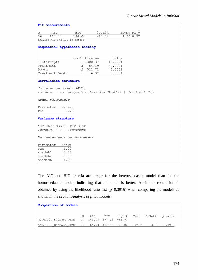
Linear Mixed Models in InfoStat
174
Fit measurements
N AIC BIC logLik Sigma R2_0
36 164.03 184.06 -65.02 4.20 0.97 Smaller AIC and BIC is better
Sequential hypothesis testing
numDF F-value p-value
(Intercept) 1 4300.37 <0.0001
Treatment 3 54.19 <0.0001
Depth 2 511.72 <0.0001
Treatment:Depth 6 6.32 0.0004
Correlation structure
Correlation model: AR(1)
Formula: ~ as.integer(as.character(Depth)) | Treatment_Rep
Model parameters
Parameter Estim.
Phi 0.73
Variance structure
Variance model: varIdent
Formula: ~ 1 | Treatment
Variance-function parameters
Parameter Estim
sun 1.00
shadeL1 0.65
shadeL2 0.66
shadeNL 1.22
The AIC and BIC criteria are larger for the heteroscedastic model than for the
homoscedastic model, indicating that the latter is better. A similar conclusion is
obtained by using the likelihood ratio test (p=0.3916) when comparing the models as
shown in the section Analysis of fitted models.
Comparison of models
df AIC BIC logLik Test L.Ratio p-value
model001_Biomass_REML 14 161.03 177.52 -66.52
model002_Biomass_REML 17 164.03 184.06 -65.02 1 vs 2 3.00 0.3916

Linear Mixed Models in InfoStat
175
For this reason, we selected the homoscedastic model, and because there is interaction
between the two factors, we generate a scatter plot to visualize the behavior of the worm
biomass means (Figure 118).
Figure 118: Dot plot used to study the interaction between Treatments and Depth and its effect on
biomass (Earthworms.IDB2 file).
As shown, this graph suggests the presence of linear behavior for sun and quadratic
behavior for the other treatments. To test these hypotheses, orthogonal and polynomial
contrasts are conducted, from the Comparison tab, Contrasts subtab (Figure 119).
Shade_L1 Shade_L2 Shade_NL Sun
1 2 3
Depth
20
30
40
50
60
70
80
90
Bio
ma
ss
Shade_L1 Shade_L2 Shade_NL Sun

Linear Mixed Models in InfoStat
176
Figure 119: Window displaying the Comparisons tab and Contrasts subtab for evaluating a mixed
model (Earthworms.IDB2 file).
The results of the contrasts are shown below. The only treatment that shows only a
linear trend, and no quadratic trend, is the sun treatment (p<0.0001 and p=0.8147
respectively). The rest of the treatments show a quadratic trend in addition to a linear
trend.
hypothesis testing for contrasts
Treatment*Depth F df(num) df(den) p-value
Ct.1 111.81 1 24 <0.0001
Ct.2 0.06 1 24 0.8147
Ct.3 222.11 1 24 <0.0001
Ct.4 26.66 1 24 <0.0001
Ct.5 164.40 1 24 <0.0001
Ct.6 10.52 1 24 0.0035
Ct.7 92.62 1 24 <0.0001
Ct.8 7.26 1 24 0.0127
Total 79.43 8 24 <0.0001

Linear Mixed Models in InfoStat
177
Contrasts coefficients
Treatment Depth Ct.1 Ct.2 Ct.3 Ct.4 Ct.5 Ct.6 Ct.7 Ct.8
sun 1 -1.00 1.00 0.00 0.00 0.00 0.00 0.00 0.00
sun 2 0.00 -2.00 0.00 0.00 0.00 0.00 0.00 0.00
sun 3 1.00 1.00 0.00 0.00 0.00 0.00 0.00 0.00
shadeL1 1 0.00 0.00 -1.00 1.00 0.00 0.00 0.00 0.00
shadeL1 2 0.00 0.00 0.00 -2.00 0.00 0.00 0.00 0.00
shadeL1 3 0.00 0.00 1.00 1.00 0.00 0.00 0.00 0.00
shadeL2 1 0.00 0.00 0.00 0.00 -1.00 1.00 0.00 0.00
shadeL2 2 0.00 0.00 0.00 0.00 0.00 -2.00 0.00 0.00
shadeL2 3 0.00 0.00 0.00 0.00 1.00 1.00 0.00 0.00
shadeNL 1 0.00 0.00 0.00 0.00 0.00 0.00 -1.00 1.00
shadeNL 2 0.00 0.00 0.00 0.00 0.00 0.00 0.00 -2.00
shadeNL 3 0.00 0.00 0.00 0.00 0.00 0.00 1.00 1.00

Linear Mixed Models in InfoStat
178
Augmented design with replicated checks
This type of treatment arrangement is common in the evaluation of new cultivars
(varieties, hybrids, etc.) in genetic plant breeding. Essentially, it consists of randomly
locating the group of cultivars to be evaluated and always inserting a common control
between the groups. The presence of this control allows us to model the systematic
effects of soil quality where the experimental plots are located. An example with 16
hybrids (H1, ..., H16) and one control, for a total of 32 experimental units, is presented.
The data are in the file Matched checks.IDB2.
A basic alternative for analyzing these data (that is not very efficient) is to conduct a
one-way ANOVA in order to compare treatments using an estimation of the error term
based on the variance between the controls (the only levels of the treatment factor that
are repeated). This model is not able to take into account the bias produced by the
systematic difference between experimental units. In order to fit this model, specify
Yield as the dependent variable in the variables selector and Hybrid as the classification
variable.
In the Fixed effects tab, Hybrid was specified as shown in Figure 120. Then, in the
Comparisons tab, Fisher’s LSD test for Hybrid was requested.

Linear Mixed Models in InfoStat
179
Figure 120: Window displaying the Fixed effects tab (Matched checks.IDB2 file).
The corresponding results are shown below.
Extended and mixed linear models
R specification of the model
model001_Yield_REML<-gls(Yield~1+Hybrid
,method="REML"
,na.action=na.omit
,data=R.data01)
Results for model: model001_Yield_REML
Dependent variable:Yield
Fit measurements
N AIC BIC logLik Sigma R2_0
32 219.90 232.64 -91.95 101.35 0.69 Smaller AIC and BIC is better

Linear Mixed Models in InfoStat
180
Sequential hypothesis testing
numDF F-value p-value
(Intercept) 1 3580.56 <0.0001
Hybrid 16 2.12 0.0763
Adjusted means and standard error for Hybrid
LSD Fisher (alpha=0.05)
p-value correction procedure: No
Hybrid Means S.E.
H4 1230.00 101.35 A
H3 1222.00 101.35 A
H14 1193.00 101.35 A B
H10 1168.00 101.35 A B C
H11 1116.00 101.35 A B C
Witness 1115.81 25.34 A B C
H5 1099.00 101.35 A B C
H9 1063.00 101.35 A B C
H2 1037.00 101.35 A B C D
H12 1033.00 101.35 A B C D
H8 975.00 101.35 A B C D
H7 966.00 101.35 A B C D
H16 928.00 101.35 A B C D
H6 907.00 101.35 B C D
H1 886.00 101.35 C D
H13 876.00 101.35 C D
H15 756.00 101.35 D
Means with a common letter are not significantly different (p<= 0.05)
The F trial for Hybrid was not significant (p = 0.0763), thus the differences between
means presented by Fisher’s LSD test should not be interpreted.
Alternatively, it is possible to use spatial correlations to correct the means of each
hybrid for the “site effect” of the location to which they were randomly assigned. To do
this, we proceed to specify plot Position as a covariate.
The Fixed effects tab should look as in Figure 120. In the Correlation tab, the following
different models should be specified:
Model 1: Exponential spatial correlation (Figure 121).
Model 2: Gaussian spatial correlation (Figure 122).
Model 3: Linear spatial correlation (Figure 123).
Model 4: “Rational quadratic” spatial correlation (Figure 124).
Model 5: Spherical spatial correlation (Figure 125).

Linear Mixed Models in InfoStat
181
The spatial correlation selection windows and the fit measures for each of the estimated
models are shown below.
Figure 121: Window displaying the Correlation tab, and selection of Exponential spatial correlation
(Matched checks.IDB2 file).
Fit measurements
N AIC BIC logLik Sigma R2_0
32 218.62 232.08 -90.31 112.79 0.58 Smaller AIC and BIC is better
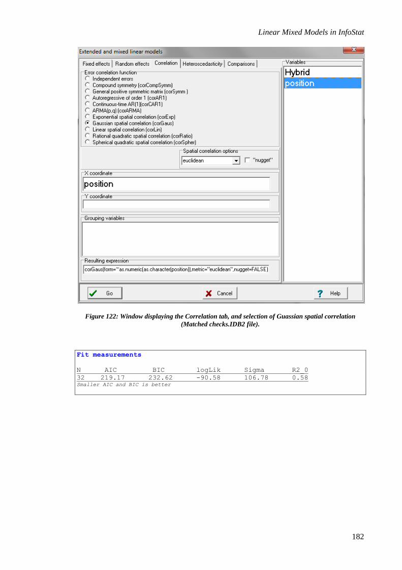
Linear Mixed Models in InfoStat
182
Figure 122: Window displaying the Correlation tab, and selection of Guassian spatial correlation
(Matched checks.IDB2 file).
Fit measurements
N AIC BIC logLik Sigma R2_0
32 219.17 232.62 -90.58 106.78 0.58 Smaller AIC and BIC is better

Linear Mixed Models in InfoStat
183
Figure 123: Window displaying the Correlation tab, and selection of Linear spatial correlation
(Matched checks.IDB2 file).
Fit measurements
N AIC BIC logLik Sigma R2_0
32 219.13 232.58 -90.56 107.52 0.56 Smaller AIC and BIC is better

Linear Mixed Models in InfoStat
184
Figure 124: Window displaying the Correlation tab, and selection of “Rational quadratic” spatial
correlation (Matched checks.IDB2 file).
Fit measurements
N AIC BIC logLik Sigma R2_0
32 218.81 232.26 -90.40 106.92 0.59 Smaller AIC and BIC is better
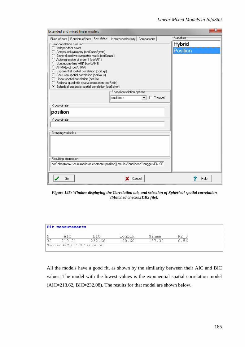
Linear Mixed Models in InfoStat
185
Figure 125: Window displaying the Correlation tab, and selection of Spherical spatial correlation
(Matched checks.IDB2 file).
Fit measurements
N AIC BIC logLik Sigma R2_0
32 219.21 232.66 -90.60 137.39 0.56 Smaller AIC and BIC is better
All the models have a good fit, as shown by the similarity between their AIC and BIC
values. The model with the lowest values is the exponential spatial correlation model
(AIC=218.62, BIC=232.08). The results for that model are shown below.
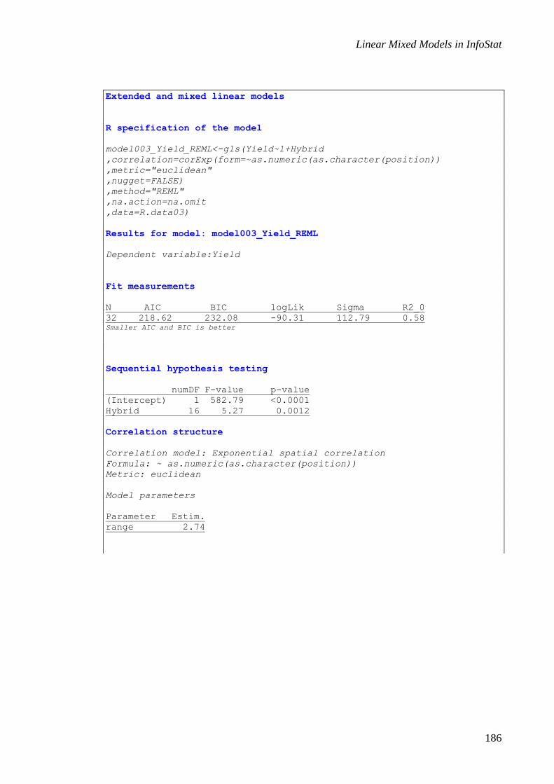
Linear Mixed Models in InfoStat
186
Extended and mixed linear models
R specification of the model
model003_Yield_REML<-gls(Yield~1+Hybrid
,correlation=corExp(form=~as.numeric(as.character(position))
,metric="euclidean"
,nugget=FALSE)
,method="REML"
,na.action=na.omit
,data=R.data03)
Results for model: model003_Yield_REML
Dependent variable:Yield
Fit measurements
N AIC BIC logLik Sigma R2_0
32 218.62 232.08 -90.31 112.79 0.58 Smaller AIC and BIC is better
Sequential hypothesis testing
numDF F-value p-value
(Intercept) 1 582.79 <0.0001
Hybrid 16 5.27 0.0012
Correlation structure
Correlation model: Exponential spatial correlation
Formula: ~ as.numeric(as.character(position))
Metric: euclidean
Model parameters
Parameter Estim.
range 2.74

Linear Mixed Models in InfoStat
187
Adjusted means and standard error for Hybrid
LSD Fisher (alpha=0.05)
p-value correction procedure: No
Hybrid Means S.E.
H3 1248.31 85.33 A
H4 1244.19 85.33 A
H10 1145.64 85.33 A B
H5 1128.65 85.33 A B C
Witness 1096.98 45.09 A B C
H2 1091.07 85.33 A B C
H11 1078.43 85.33 A B C
H9 1078.28 85.33 A B C
H14 1070.07 85.33 A B C
H1 1005.46 85.33 B C
H12 979.80 85.33 B C
H6 966.31 85.33 B C
H7 936.21 85.33 B C D
H8 933.40 85.33 B C D
H16 902.87 85.33 C D
H13 727.55 85.33 D E
H15 653.36 85.33 E
Means with a common letter are not significantly different (p<= 0.05)
Differences between hybrids were found (p = 0.0012). Fisher’s LSD means comparison
shows that the hybrids with the greatest yield are H2, H3, H4, H5, H9, H10, H11, H14,
and that these do not differ from the control.
Alternatively, the problem can be thought of as it might have been during the early days
of spatial correlation modeling (Papadakis 1937), and one might use covariance analysis
to adjust the means of the hybrids in the different positions. In order to approximate this
type of analysis, we created a new variable called Tes, which contains the yields
corresponding to the hybrid closest to each control. Then, the difference between the
control yield and the hybrid yield (Dif) was calculated.
We then conducted a linear regression analysis, with Dif as the dependent variable and
position as the regressor. The predicted values of this model were saved with the
intention of using them as covariates in the analysis of the hybrid means. Then, in the
Extended and mixed linear models variables selector window, variables are specified as
shown in Figure 126.

Linear Mixed Models in InfoStat
188
Figure 126: Variables selector window for the Extended and mixed linear models (Matched
checks.IDB2 file).
In the fixed effects window, declare PRED_Dif and Hybrid. The corresponding output
is shown below.
Extended and mixed linear models
R specification of the model
model004_Yield_REML<-gls(Yield~1+Hybrid+PRED_Dif
.method="REML"
.na.action=na.omit
.data=R.data04)
Results for model: model004_Yield_REML
Dependent variable:Yield
Fit measurements
N AIC BIC logLik Sigma R2_0
32 215.09 227.23 -88.54 79.89 0.82 Smaller AIC and BIC is better
Sequential hypothesis testing
numDF F-value p-value
(Intercept) 1 5763.58 <0.0001
Hybrid 16 3.42 0.0129
PRED_Dif 1 10.15 0.0066

Linear Mixed Models in InfoStat
189
Adjusted means and standard error for Hybrid
LSD Fisher (alpha=0.05)
p-value correction procedure: No
Hybrid Means S.E.
H4 1295.07 82.46 A
H3 1293.92 83.02 A
H10 1150.88 80.07 A B
H5 1143.52 81.10 A B
H2 1129.47 85.00 A B
H14 1121.08 83.02 A B
Witness 1115.81 19.97 A B
H11 1078.33 80.76 A B
H9 1052.73 79.95 A B C
H12 988.48 81.10 B C
H1 985.32 85.76 B C
H8 985.27 79.95 B C
H7 983.12 80.07 B C
H6 944.67 80.76 B C
H16 828.68 85.76 C D
H13 810.93 82.46 C D
H15 663.53 85.00 D Means with a common letter are not significantly different (p<= 0.05)
Although the conclusion regarding the cultivars is the same as that of the exponential
spatial correlation analysis, we can observe that the adjusted means and the standard
errors are different. The order, or ranking, among the hybrids that generated the greatest
yields is also different. Furthermore, studying spatial correlation is a much simpler
alternative to conduct this type of analysis.
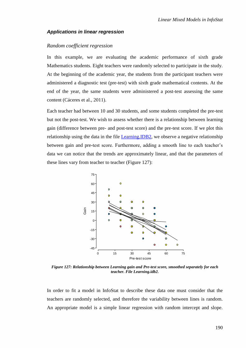
Linear Mixed Models in InfoStat
190
Applications in linear regression
Random coefficient regression
In this example, we are evaluating the academic performance of sixth grade
Mathematics students. Eight teachers were randomly selected to participate in the study.
At the beginning of the academic year, the students from the participant teachers were
administered a diagnostic test (pre-test) with sixth grade mathematical contents. At the
end of the year, the same students were administered a post-test assessing the same
content (Cáceres et al., 2011).
Each teacher had between 10 and 30 students, and some students completed the pre-test
but not the post-test. We wish to assess whether there is a relationship between learning
gain (difference between pre- and post-test score) and the pre-test score. If we plot this
relationship using the data in the file Learning.IDB2, we observe a negative relationship
between gain and pre-test score. Furthermore, adding a smooth line to each teacher’s
data we can notice that the trends are approximately linear, and that the parameters of
these lines vary from teacher to teacher (Figure 127):
Figure 127: Relationship between Learning gain and Pre-test score, smoothed separately for each
teacher. File Learning.idb2.
In order to fit a model in InfoStat to describe these data one must consider that the
teachers are randomly selected, and therefore the variability between lines is random.
An appropriate model is a simple linear regression with random intercept and slope.
0 15 30 45 60 75
Pre-test score
-45
-30
-15
0
15
30
45
60
75
Ga
in

Linear Mixed Models in InfoStat
191
These random effects must clearly be correlated (in general, if the slope increases the
intercept should decrease for the data to stay in the same observed area). Hence, the
model must be specified in InfoStat in such a way that correlated intercept and slope
random effects can be incorporated. To do this, in the Variables window we need to
select Gain as variable, Teacher as class variable, and Pre-test score as covariate. Then,
in the Fixed effect tab, Pre-test score is selected, and we need to add the explicit
specification of the intercept (to be able to declare both as random effects later). This is
done adding 1 in the Fixed effects tab (Figure 128). We also need to check the option
Fixed effects coefficients to obtain the equation of the average line.
Figure 128: Window to select fixed effects in the Extended and mixed models for the data in the file
LearningIDB2.

Linear Mixed Models in InfoStat
192
The specification of the random effects is done by adding Teacher as stratification
criterion, and indicating that this effects acts on 1+Pre.test (i.e., there are random
teacher effects on the intercept and on the slope) (Figure 129). Furthermore, it is
necessary to indicate pdSymm as the covariance structure of these random effects in
order to have different variances for intercept and slope (obvious given the different
nature of both parameters), and correlation between both random effects
Figure 129: Extended and mixed linear models with the Random effects tab for the data in the file
Learning.IDB2.
The output for this model shows, in addition to the usual parts in mixed models, the
coefficients of the average straigth line, ˆ 30.13 0.81Y x . As expected, as the pre-test
score is larger the gain decreases. One can also notice the large correlation between
intercept and slope (-0.876), which confirms the need to incorporate this parameter in
the model.

Linear Mixed Models in InfoStat
193
Extended and mixed linear models
R specification of the model
model.008_Gain_REML<-lme(Gain~1+Pre.test.score
,random=list(Teacher=pdSymm(~1+Pre.test.score))
,method="REML"
,control=lmeControl(msMaxIter=200)
,na.action=na.omit
,data=R.data08
,keep.data=FALSE)
Results for model: model.008_Gain_REML
Dependent variable: Gain
Fit measurements
N AIC BIC logLik Sigma R2_0 R2_1
184 1485.954 1505.178 -736.977 13.174 0.339 0.366 Smaller AIC and BIC is better
Marginal hypothesis testingmodel.008_Gain_REML
numDF denDF F-value p-value
(Intercept) 1 175 104.797 <0.0001
Pre.test.score 1 175 78.129 <0.0001
Sequential hypothesis testing
numDF denDF F-value p-value
(Intercept) 1 175 29.007 <0.0001
Pre.test.score 1 175 78.129 <0.0001
Fixed effects
Value Std.Error DF t-value p-value
(Intercept) 30.133 2.944 175 10.237 <0.0001
Pre.test.score -0.811 0.092 175 -8.839 <0.0001
Random effects parameters
Covariance model for random effects: pdSymm
Formula: ~1 + Pre.test.score|Teacher
Standard deviations and correlations
(const) Pre.test.score
(const) 2.645 -0.876
Pre.test.score -0.876 0.111

Linear Mixed Models in InfoStat
194
Heteroscedastic regression
In a research to evaluate primary productivity in pastures and its relationship with
precipitation, nine plots were evaluated (five with native pasture and four with sown
pastures). The primary productivity for 22-day periods was measured several times
during the year in each plot (most plots were measures 12 times). Simultaneously,
rainfall (mm) during the 22-days growing period was recorded (Ospina 2011, Ospina et
al. 2012). The data are in the file Primary productivity.IDB2. In order to make a
regression analysis including pasture as a classification variable, we select the variables
in the Extended and mixed linear models module as shown in Figure 130.
Figure 130: Variable selection window in the Extended and mixed linear models module for the data
in file Primary productivity.IDB2.
In the Fixed effects tab we select the variables as in Figure 131 and in the Random
effects tab we select Plot (Figure 132). With these specifications we are fitting a linear
regression model with two intercepts (one for native and one for sown pastures), and a
random plot effect. The residuals obtained from fitting this model can be used to

Linear Mixed Models in InfoStat
195
diagnose possible problems. In Figure 133 the q-q plot shows that the residuals
distribution is approximately normal, but the scatterplot of Pearson conditional residuals
vs. Rain shows a runs of negative residual values beyond 300 mm. This same run is
observed in the scatterplot of Pearson conditional residual vs. fitted values, in this case
beyond 110 g of primary productivity. This suggests the need to add a quadratic term
for the regression Rain. To do this, in the Data menu, Transformations submenu, select
Rain as variable. Then request a power transformation (in this case of order 2), and this
generates a new variable in the dataset call POW_Rain.
Figure 131: Window from the Extended and mixed linear model with the Fixed effects tab for the data
in file Primary productivity.IDB2.

Linear Mixed Models in InfoStat
196
Figure 132: Window from the Extended and mixed linear model with the Random effects tab for the
data in file Primary productivity.IDB2.

Linear Mixed Models in InfoStat
197
Figure 133: Graphical tools for diagnostic obtained from the data in file Primary productivity.IDB2
with Rain as regressor and Pasture as fixed factor.
The variable POW_Rain was added as covariate in the variable selector window in
Extended and mixed linear models. Then it was included in the Fixed effects tab in the
model, together with the other variables already entered as shown in Figure 142. The
random effects tab is left unchanged as in Figure 132. Once this model is fitted and the
residual diagnostic is requested, we obtain the plots shown in Figure 134.

Linear Mixed Models in InfoStat
198
Figure 134: Graphical tools for diagnostic obtained from the data in file Primary productivity.IDB2
with Rain and POW_Rain as regressors and Pasture as fixed factor.
Analyzing the scatter plot of Pearson conditional residuals vs. fitted values, we notice a
clear trend for the residuals to increase their variance as their mean value increases. This
suggests the need to model the variance heterogeneity with a function relating the
residual variances with the mean. To use this function, we run the analysis again
(remember that CTRL + r repeats the last command in InfoStat), and in the
Heteroscedasticity tab we add VarPower as shown in Figure 135.
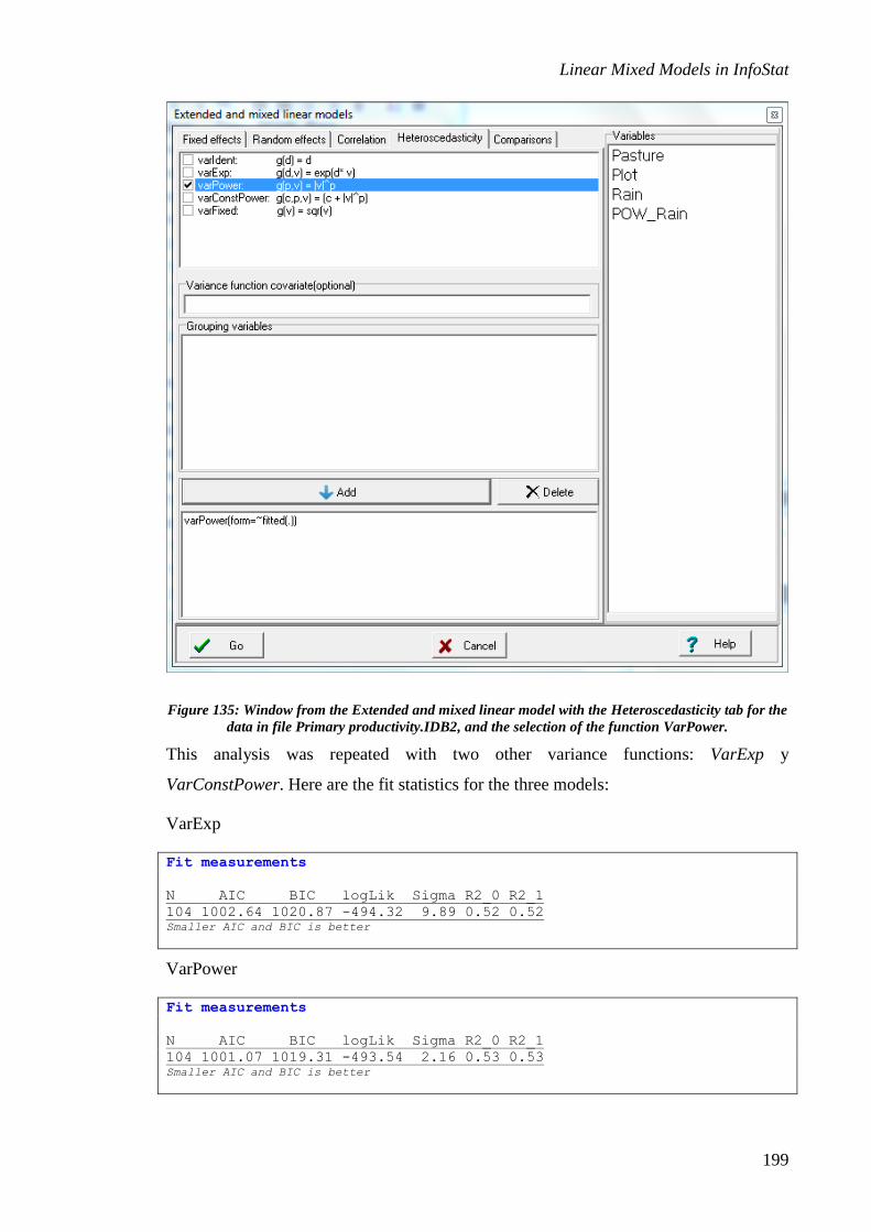
Linear Mixed Models in InfoStat
199
Figure 135: Window from the Extended and mixed linear model with the Heteroscedasticity tab for the
data in file Primary productivity.IDB2, and the selection of the function VarPower.
This analysis was repeated with two other variance functions: VarExp y
VarConstPower. Here are the fit statistics for the three models:
VarExp
Fit measurements
N AIC BIC logLik Sigma R2_0 R2_1
104 1002.64 1020.87 -494.32 9.89 0.52 0.52 Smaller AIC and BIC is better
VarPower
Fit measurements
N AIC BIC logLik Sigma R2_0 R2_1
104 1001.07 1019.31 -493.54 2.16 0.53 0.53 Smaller AIC and BIC is better

Linear Mixed Models in InfoStat
200
VarConstPower
Fit measurements
N AIC BIC logLik Sigma R2_0 R2_1
104 1001.85 1022.69 -492.92 0.62 0.52 0.52 Smaller AIC and BIC is better
We cannot compare these models using likelihood ratio tests because they do not form a
nested set of hypotheses (except VarPower and VarConstPower). In these cases only
the AIC and BIC criteria are useful. The model VarPower results the best alternative to
model the variance heterogeneity. After fitting this model, residuals do not show any
trend (Figure 136).
Figure 136: Graphical tools for diagnostic obtained from the data in file Primary productivity.IDB2
with Rain and POW.Rain as regressors, Pasture as fixed factor, and a VarPower function to model
variance heterogeneity.

Linear Mixed Models in InfoStat
201
To test the hypothesis of equal linear and quadratic trends for both pastures, we
included in the model the interactions between pasture type and the two regressors
(Figure 137). The random plot effect was added in the Random effects tab (Figure 138)
and the heteroscedasticity was specified as in Figure 135.
Figure 137: Window from the Extended and mixed linear model for the data in file Primary
productivity.IDB2, and the specification of the model with interaction.
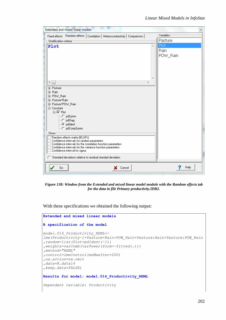
Linear Mixed Models in InfoStat
202
Figure 138: Window from the Extended and mixed linear model module with the Random effects tab
for the data in file Primary productivity.IDB2.
With these specifications we obtained the following output:
Extended and mixed linear models
R specification of the model
model.014_Productivity_REML<-
lme(Productivity~1+Pasture+Rain+POW_Rain+Pasture:Rain+Pasture:POW_Rain
,random=list(Plot=pdIdent(~1))
,weights=varComb(varPower(form=~fitted(.)))
,method="REML"
,control=lmeControl(msMaxIter=200)
,na.action=na.omit
,data=R.data14
,keep.data=FALSE)
Results for model: model.014_Productivity_REML
Dependent variable: Productivity

Linear Mixed Models in InfoStat
203
Fit measurements
N AIC BIC logLik Sigma R2_0 R2_1
104 1004.89 1028.15 -493.45 2.46 0.65 0.65 Smaller AIC and BIC is better
Marginal hypothesis testing (Type III SS)
numDF denDF F-value p-value
(Intercept) 1 91 0.32 0.5703
Pasture 1 7 12.62 0.0093
Rain 1 91 167.15 <0.0001
POW_Rain 1 91 55.66 <0.0001
Pasture:Rain 1 91 4.19 0.0435
Pasture:POW_Rain 1 91 0.01 0.9179
Sequential hypothesis testing
numDF denDF F-value p-value
(Intercept) 1 91 152.56 <0.0001
Pasture 1 7 34.31 0.0006
Rain 1 91 184.34 <0.0001
POW_Rain 1 91 62.10 <0.0001
Pasture:Rain 1 91 21.04 <0.0001
Pasture:POW_Rain 1 91 0.01 0.9179
Fixed effects
Value Std.Error DF t-value p-value
(Intercept) 6.83 3.67 91 1.86 0.0660
PastureSown -16.27 4.58 7 -3.55 0.0093
Rain 0.60 0.07 91 8.32 <0.0001
POW_Rain -1.0E-03 1.8E-04 91 -5.74 <0.0001
PastureSown:Rain 0.23 0.11 91 2.05 0.0435
PastureSown:POW_Rain -2.9E-05 2.8E-04 91 -0.10 0.9179
Random effects parameters
Covariance model for random effects: pdIdent
Formula: ~1|Plot
Standard deviations and correlations
(const)
(const) 1.3E-03
Variance structure
Variance model: varPower
Formula: ~ fitted(.)
Variance-function parameters
Parameter Estim.
power 0.60
As can be seen from the previous output, there is interaction of pasture with rain, which
indicates that the linear component is different in both pastures. On the other hand, there

Linear Mixed Models in InfoStat
204
are no differences in the quadratic component and hence it is the same in both pastures.
The final model eliminated the interaction Pasture*POW_Rain, and the resulting output
follows.
Extended and mixed linear models
R specification of the model
model.015_Productivity_REML<-
lme(Productivity~1+Pasture+Rain+POW_Rain+Pasture:Rain
,random=list(Plot=pdIdent(~1))
,weights=varComb(varPower(form=~fitted(.)))
,method="REML"
,control=lmeControl(msMaxIter=200)
,na.action=na.omit
,data=R.data15
,keep.data=FALSE)
Results for model: model.015_Productivity_REML
Dependent variable: Productivity
Fit measurements
N AIC BIC logLik Sigma R2_0 R2_1
104 988.37 1009.14 -486.19 2.46 0.65 0.65 Smaller AIC and BIC is better
Marginal hypothesis testing (Type III SS)
numDF denDF F-value p-value
(Intercept) 1 92 0.35 0.5579
Pasture 1 7 17.01 0.0044
Rain 1 92 171.84 <0.0001
POW_Rain 1 92 57.67 <0.0001
Pasture:Rain 1 92 21.17 <0.0001
Sequential hypothesis testing
numDF denDF F-value p-value
(Intercept) 1 92 154.21 <0.0001
Pasture 1 7 33.77 0.0007
Rain 1 92 186.37 <0.0001
POW_Rain 1 92 63.32 <0.0001
Pasture:Rain 1 92 21.17 <0.0001
Fixed effects
Value Std.Error DF t-value p-value
(Intercept) 6.66 3.43 92 1.94 0.0553
PastureSown -16.00 3.88 7 -4.12 0.0044
Rain 0.60 0.06 92 10.42 <0.0001
POW_Rain -1.0E-03 1.4E-04 92 -7.59 <0.0001
PastureSown:Rain 0.21 0.05 92 4.60 <0.0001

Linear Mixed Models in InfoStat
205
Random effects parameters
Covariance model for random effects: pdIdent
Formula: ~1|Plot
Standard deviations and correlations
(const)
(const) 2.2E-03
Variance structure
Variance model: varPower
Formula: ~ fitted(.)
Variance-function parameters
Parameter Estim.
power 0.60
Adjusted means and standard error for Pasture
LSD Fisher (Alpha:=0.05)
p-value correction procedure: No
Pasture Means S.E.
Sown 70.01 4.58 A
Semi-natural 56.17 3.52 B Means with a common letter are not significantly different (p<= 0.05)
Due to the presence of a polynomial regression, it is more appropriate to report
sequential tests (type I). We can conclude that there is a pasture effect (p=0.0007), a
rain quadratic effect (p<0.0001), and a difference in linear trend between pastures
(p<0.0001). Figure 139 shows the estimated average lines and the observations at
individual plots.

Linear Mixed Models in InfoStat
206
Figure 139: Scatterplot showing the relationship between primary productivity and rain for each of the
two pastures. File Primary productivity.IDB2.
Since there is interaction, it is not possible to interpret the adjusted means. In order to
compare both pastures at a given level of rain we can use the menu Model Exploration,
Linear combinations tab. To determine the coefficients to be used, consider the
following hypothesis (which tests if there are differences in primary productivity of
both pastures for a cumulative rain of 100 mm):
0 0 1 2 0 1 2 1: 100 10000 100 10000 100H
This hypothesis is equivalent to 0 1: 100 0H , which is expressed as a linear
combination of parameters in the model . Similarly, it is possible to contrast pastures at
other rain levels. The coefficients to do for 100 mm, 300 mm and 500 mm are shown in
Figure 140.
Native
Sow n
0 50 100 150 200 250 300 350 400 450 500 550 600
Rain
0
20
40
60
80
100
120
140
160
180
200
Pri
ma
ry p
rod
uctivity
Native
Sow n
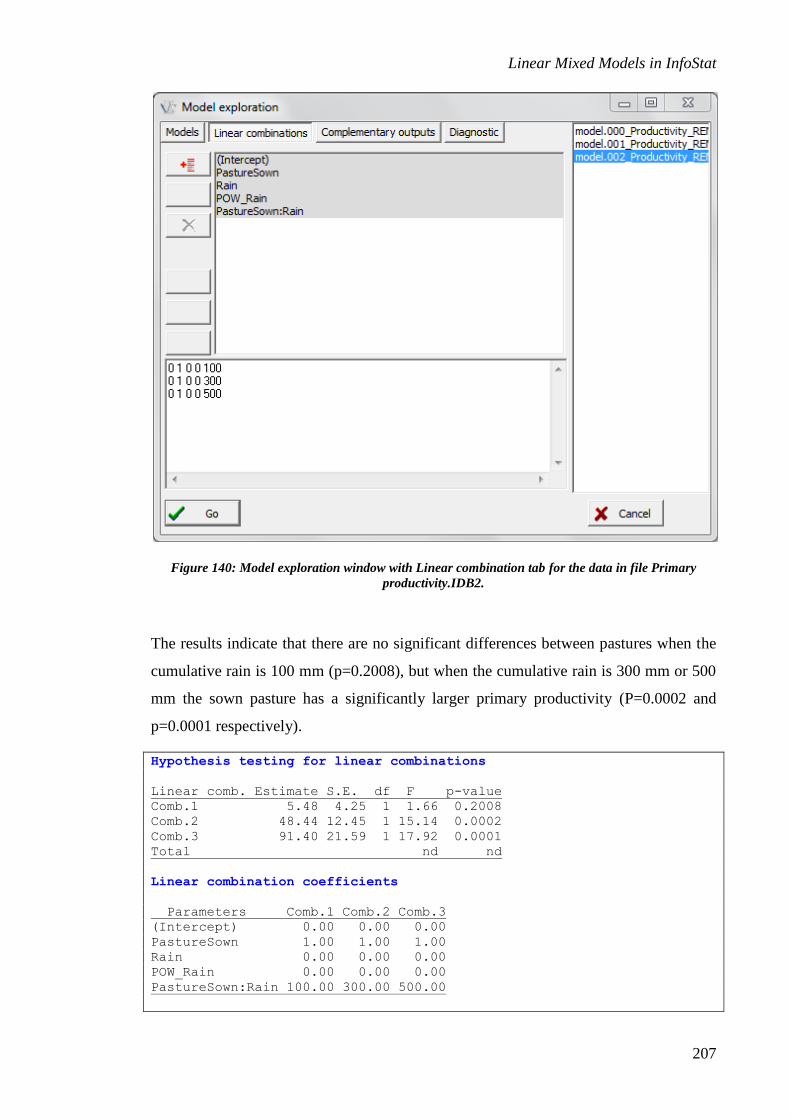
Linear Mixed Models in InfoStat
207
Figure 140: Model exploration window with Linear combination tab for the data in file Primary
productivity.IDB2.
The results indicate that there are no significant differences between pastures when the
cumulative rain is 100 mm (p=0.2008), but when the cumulative rain is 300 mm or 500
mm the sown pasture has a significantly larger primary productivity (P=0.0002 and
p=0.0001 respectively).
Hypothesis testing for linear combinations
Linear comb. Estimate S.E. df F p-value
Comb.1 5.48 4.25 1 1.66 0.2008
Comb.2 48.44 12.45 1 15.14 0.0002
Comb.3 91.40 21.59 1 17.92 0.0001
Total nd nd
Linear combination coefficients
Parameters Comb.1 Comb.2 Comb.3
(Intercept) 0.00 0.00 0.00
PastureSown 1.00 1.00 1.00
Rain 0.00 0.00 0.00
POW_Rain 0.00 0.00 0.00
PastureSown:Rain 100.00 300.00 500.00

Linear Mixed Models in InfoStat
208
Incomplete blocks and related designs
Alpha lattice designs
The data from this example come from an 18-variety barley trial conducted in Scotland
(Patterson et al., 1989). Due to the large number of treatments, it was impossible to find
blocks with 18 homogenous experimental units, and hence the blocks were incomplete
(Data: Alpha lattice.IDB2). A complete replication for this experiment consists of 3
incomplete blocks with 4 experimental units each, and 2 blocks with 3 units each. There
was a total of 4 replications (Figure 141).
1
11
1
3
1
8
1
10
2
13
2
17
2
16
2
5
3
14
3
18
3
4
4
6
4
1
4
7
4
12
5
9
5
2
5
15
I
1
15
1
4
1
11
1
17
2
5
2
12
2
10
3
9
3
1
3
13
4
2
4
14
4
7
4
8
5
16
5
6
5
3
5
18
II
1
12
1
15
1
3
2
4
2
16
2
7
3
8
3
4
3
12
3
13
4
18
4
8
4
5
4
9
5
10
5
17
5
14
5
1
III
1
10
1
2
1
16
2
9
2
17
2
7
2
3
3
8
3
4
3
12
3
13
4
15
4
6
4
5
4
14
5
11
5
1
5
18
IV
Figure 141: Layout of the design for the 18-variety barley trial conducted in an alpha-lattice. Roman
numbers at the right indicate replicates, arabic numbers at the top of each cell indicate the incomplete
block (of sizes 4 and 3), and numbers at the bottom of each cell represent the varieties.
The first analysis will be done considering only the repetitions as whole (complete)
blocks. Since there are 4 repetitions, an error term for the comparisons can be estimated.
In the variable selection window in Extended and mixed linear models we select Yield
as variable, Variety, Incomplete block and Repetition as class variables. After this, we
select Variety in the Fixed effects tab (Figure 142), and Repetition in the Random effect
tab (Figure 143). Since all the varieties are present in each repetition, this form corrects
for possible repetition bias, although it ignores the incomplete block effects (and hence
the possible bias due to incomplete blocks).
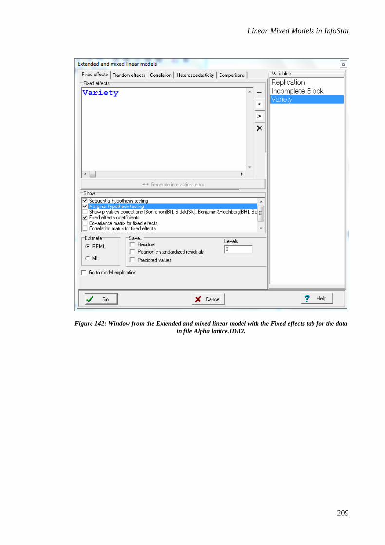
Linear Mixed Models in InfoStat
209
Figure 142: Window from the Extended and mixed linear model with the Fixed effects tab for the data
in file Alpha lattice.IDB2.

Linear Mixed Models in InfoStat
210
Figure 143: Window from the Extended and mixed linear model with the Random effects tab and the
Replication effect for the data in file Alpha lattice.IDB2.
The following output shows the result from this model.
Extended and mixed linear models
R specification of the model
model.002_Yield_REML<-lme(Yield~1+Variety
,random=list(Replication=pdIdent(~1))
,method="REML"
,control=lmeControl(msMaxIter=200)
,na.action=na.omit
,data=R.data02
,keep.data=FALSE)
Results for model: model.002_Yield_REML
Dependent variable: Yield
Fit measurements
N AIC BIC logLik Sigma R2_0 R2_1
72 65.28 105.06 -12.64 0.22 0.37 0.70 Smaller AIC and BIC is better

Linear Mixed Models in InfoStat
211
Marginal hypothesis testing (Type III SS)
numDF denDF F-value p-value
(Intercept) 1 51 1977.36 <0.0001
Variety 17 51 3.74 0.0001
Sequential hypothesis testing
numDF denDF F-value p-value
(Intercept) 1 51 1977.36 <0.0001
Variety 17 51 3.74 0.0001
Fixed effects
Value Std.Error DF t-value p-value
(Intercept) 5.33 0.16 51 33.73 <0.0001
Variety10 -0.68 0.16 51 -4.27 0.0001
Variety11 -0.20 0.16 51 -1.26 0.2118
Variety12 -0.48 0.16 51 -3.00 0.0041
Variety13 -0.33 0.16 51 -2.05 0.0451
Variety14 0.00 0.16 51 0.00 >0.9999
Variety15 -0.05 0.16 51 -0.32 0.7532
Variety16 -0.23 0.16 51 -1.42 0.1610
Variety17 0.18 0.16 51 1.11 0.2738
Variety18 -0.48 0.16 51 -3.00 0.0041
Variety2 -0.43 0.16 51 -2.69 0.0097
Variety3 -0.08 0.16 51 -0.47 0.6374
Variety4 -0.05 0.16 51 -0.32 0.7532
Variety5 -0.38 0.16 51 -2.37 0.0216
Variety6 -0.33 0.16 51 -2.05 0.0451
Variety7 -0.20 0.16 51 -1.26 0.2118
Variety8 -0.40 0.16 51 -2.53 0.0146
Variety9 -0.13 0.16 51 -0.79 0.4330
Random effects parameters
Covariance model for random effects: pdIdent
Formula: ~1|Replication
Standard deviations and correlations
(const)
(const) 0.22
Adjusted means and standard error for Variety
LSD Fisher (Alpha:=0.05)
p-value correction procedure: No
Variety Means S.E.
17 5.50 0.16 A
14 5.33 0.16 A B
1 5.33 0.16 A B
15 5.28 0.16 A B C
4 5.28 0.16 A B C
3 5.25 0.16 A B C D
9 5.20 0.16 A B C D E
11 5.13 0.16 B C D E F
7 5.13 0.16 B C D E F
16 5.10 0.16 B C D E F
6 5.00 0.16 C D E F
13 5.00 0.16 C D E F

Linear Mixed Models in InfoStat
212
5 4.95 0.16 D E F G
8 4.93 0.16 E F G
2 4.90 0.16 E F G
18 4.85 0.16 F G
12 4.85 0.16 F G
10 4.65 0.16 G Means with a common letter are not significantly different (p<= 0.05)
As we can see, the mean comparisons are done with a single standard error (the standard
error of the estimated treatment effects, 0.1582, represent the standard error of the
difference between each treatment and the reference treatment). Now we will conduct a
new analysis incorporating the Incomplete Block effects. To do this, we leave the Fixed
effects tab as in Figure 142 (Variety) and in the Random effects tab we select Repeticion
and Incomplete Block as shown in Figure 144.
Figure 144: Window from the Extended and mixed linear model with the Random effects tab and the
Replication and Incomplete block effect for the data in file Alpha lattice.IDB2.
The following is the output corresponding to this model.

Linear Mixed Models in InfoStat
213
Extended and mixed linear models
R specification of the model
model.003_Yield_REML<-lme(Yield~1+Variety
,random=list(Replication=pdIdent(~1)
,Replication=pdIdent(~Incomplete.Block-1))
,method="REML"
,control=lmeControl(msMaxIter=200)
,na.action=na.omit
,data=R.data03
,keep.data=FALSE)
Results for model: model.003_Yield_REML
Dependent variable: Yield
Fit measurements
N AIC BIC logLik Sigma R2_0 R2_1 R2_2
72 52.35 94.12 -5.17 0.15 0.34 0.66 0.90 Smaller AIC and BIC is better
Marginal hypothesis testing (Type III SS)
numDF denDF F-value p-value
(Intercept) 1 51 2154.51 <0.0001
Variety 17 51 6.54 <0.0001
Sequential hypothesis testing
numDF denDF F-value p-value
(Intercept) 1 51 2153.76 <0.0001
Variety 17 51 6.54 <0.0001
Fixed effects
Value Std.Error DF t-value p-value
(Intercept) 5.36 0.14 51 38.82 <0.0001
Variety10 -0.74 0.12 51 -6.09 <0.0001
Variety11 -0.16 0.12 51 -1.35 0.1824
Variety12 -0.43 0.12 51 -3.55 0.0008
Variety13 -0.39 0.12 51 -3.23 0.0022
Variety14 -0.13 0.12 51 -1.04 0.3050
Variety15 -0.07 0.13 51 -0.54 0.5892
Variety16 -0.22 0.13 51 -1.75 0.0861
Variety17 0.11 0.12 51 0.94 0.3517
Variety18 -0.52 0.12 51 -4.35 0.0001
Variety2 -0.45 0.13 51 -3.57 0.0008
Variety3 -0.09 0.12 51 -0.73 0.4664
Variety4 -0.11 0.13 51 -0.84 0.4027
Variety5 -0.46 0.12 51 -3.74 0.0005
Variety6 -0.34 0.12 51 -2.83 0.0067
Variety7 -0.19 0.12 51 -1.57 0.1233
Variety8 -0.59 0.12 51 -4.76 <0.0001
Variety9 -0.27 0.12 51 -2.24 0.0292

Linear Mixed Models in InfoStat
214
Random effects parameters
Covariance model for random effects: pdIdent
Formula: ~1|Replication
Standard deviations and correlations
(const)
(const) 0.20
Covariance model for random effects: pdIdent
Formula: ~Incomplete.Block - 1|Replication
Standard deviations and correlations
S.D.
1 0.18
2 0.18
3 0.18
4 0.18
5 0.18
Adjusted means and standard error for Variety
LSD Fisher (Alpha:=0.05)
p-value correction procedure: No
Variety Means S.E.
17 5.47 0.14 A
1 5.36 0.14 A B
15 5.29 0.14 A B C
3 5.27 0.14 A B C
4 5.26 0.14 A B C D
14 5.24 0.14 A B C D
11 5.20 0.14 B C D E
7 5.17 0.14 B C D E F
16 5.14 0.14 B C D E F G
9 5.09 0.14 C D E F G H
6 5.02 0.14 D E F G H I
13 4.98 0.14 E F G H I J
12 4.93 0.14 F G H I J
2 4.91 0.14 G H I J
5 4.90 0.14 H I J
18 4.84 0.14 I J K
8 4.77 0.14 J K
10 4.62 0.14 K Means with a common letter are not significantly different (p<= 0.05)
In this output we can notice that the standard errors of the differences (=standard error
of the variety effect) are still similar for each variety, although not equal, since although
all varieties have the same number of repetitions (n=4), the incomplete blocks are of
different size (3 or 4 experimental units). Also, these standard errors are smaller than in
the previous model, since now we have eliminated the variance of blocks within each

Linear Mixed Models in InfoStat
215
replicate. The means in this last analysis are also corrected for the block effects
(adjusted means), and therefore this is a better analysis: the adjusted means are unbiased
(conditionally on the observed blocks). The mean ranking has changed: in the whole-
block-only analysis the top three means are 17, 14, and 1 respectively; while in the
incomplete block analysis the top three means were 17, 1, and 15 respectively. The
standard error of the difference of two means in the first analysis was 0.158 and in the
second analysis was 0.122 on average (in order to compute an average standard error of
differences, the usual procedure is to square each S.E., average these values, and then
take the square root of the average). The efficiency of the second analysis with respect
to the first one was:
22
0.1581.68
0.122
WholeBlocksOnly
IncompleteBlocks
SEdiffE
SEdiff
The analysis including the incomplete blocks is 68% more efficient than the one not
including this effect.
A summary of the fit measures of the two models follows. Using AIC and BIC criteria
the incomplete block analysis is better.
Incomplete block analysis
N AIC BIC logLik Sigma R2_0 R2_1 R2_2
72 52.3497 94.1184 -5.1749 0.1532 0.3431 0.6595 0.8961 Smaller AIC and BIC is better
Whole blocks only analysis
N AIC BIC logLik Sigma R2_0 R2_1
72 65.2834 105.0631 -12.6417 0.2237 0.3714 0.7015 Smaller AIC and BIC is better
Latinized row-column design
The data in this example come from a trial to evaluate 30 cotton varieties. Each variety
was repeated 5 times (William 1986). Figure 145 shows the field arrangement of the
design. Each variety is present only once in each column (latinized columns). At the

Linear Mixed Models in InfoStat
216
same time, there are groups of six rows each, containing all 30 varieties (complete
replication). These two are the randomization restrictions which must be taken into
account in the design. Notice that the rows within each repetition constitute incomplete
blocks (Lattice row column.IDB2).
To conduct the analysis in Extended and mixed linear models, select Yield as variable
and Variety, Replication, Row and Column as class variables. Then we select Variety in
the Fixed effects tab (Figure 146) and the rest of the variables in the Random effects tab,
as shown in Figure 147.
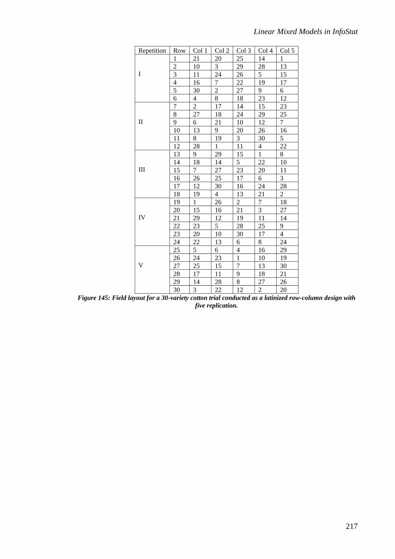
Linear Mixed Models in InfoStat
217
Repetition Row Col 1 Col 2 Col 3 Col 4 Col 5
I
1 21 20 25 14 1
2 10 3 29 28 13
3 11 24 26 5 15
4 16 7 22 19 17
5 30 2 27 9 6
6 4 8 18 23 12
II
7 2 17 14 15 23
8 27 18 24 29 25
9 6 21 10 12 7
10 13 9 20 26 16
11 8 19 3 30 5
12 28 1 11 4 22
III
13 9 29 15 1 8
14 18 14 5 22 10
15 7 27 23 20 11
16 26 25 17 6 3
17 12 30 16 24 28
18 19 4 13 21 2
IV
19 1 26 2 7 18
20 15 16 21 3 27
21 29 12 19 11 14
22 23 5 28 25 9
23 20 10 30 17 4
24 22 13 6 8 24
V
25 5 6 4 16 29
26 24 23 1 10 19
27 25 15 7 13 30
28 17 11 9 18 21
29 14 28 8 27 26
30 3 22 12 2 20
Figure 145: Field layout for a 30-variety cotton trial conducted as a latinized row-column design with
five replication.
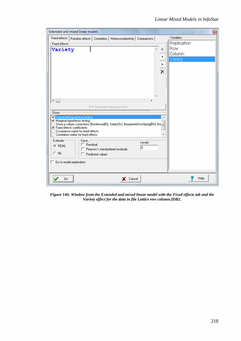
Linear Mixed Models in InfoStat
218
Figure 146: Window from the Extended and mixed linear model with the Fixed effects tab and the
Variety effect for the data in file Lattice row column.IDB2.
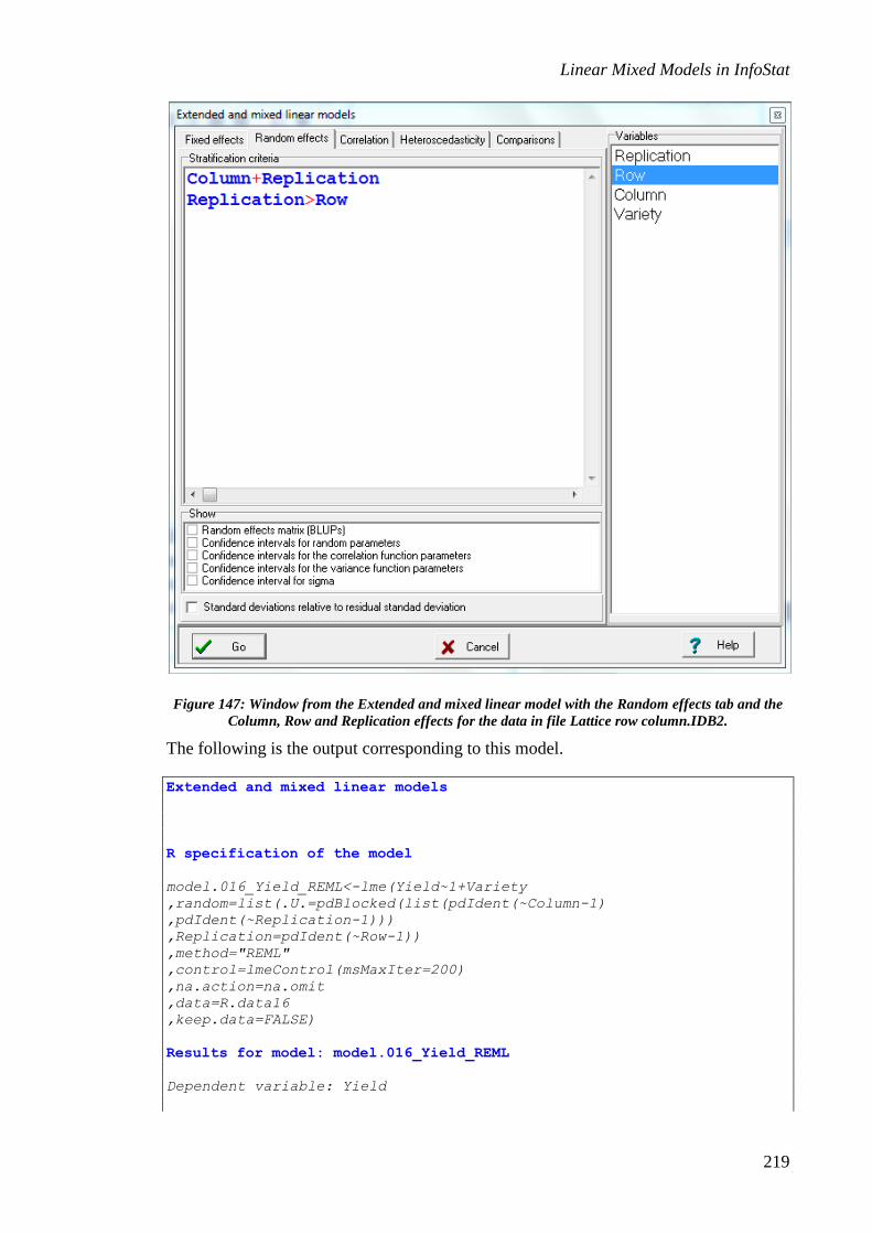
Linear Mixed Models in InfoStat
219
Figure 147: Window from the Extended and mixed linear model with the Random effects tab and the
Column, Row and Replication effects for the data in file Lattice row column.IDB2.
The following is the output corresponding to this model.
Extended and mixed linear models
R specification of the model
model.016_Yield_REML<-lme(Yield~1+Variety
,random=list(.U.=pdBlocked(list(pdIdent(~Column-1)
,pdIdent(~Replication-1)))
,Replication=pdIdent(~Row-1))
,method="REML"
,control=lmeControl(msMaxIter=200)
,na.action=na.omit
,data=R.data16
,keep.data=FALSE)
Results for model: model.016_Yield_REML
Dependent variable: Yield

Linear Mixed Models in InfoStat
220
Fit measurements
N AIC BIC logLik Sigma R2_0 R2_1 R2_2
150 1673.82 1768.59 -802.91 140.59 0.32 0.63 0.70 Smaller AIC and BIC is better
Marginal hypothesis testing (Type III SS)
numDF denDF F-value p-value
(Intercept) 1 116 1285.12 <0.0001
Variety 29 116 3.25 <0.0001
Sequential hypothesis testing
numDF denDF F-value p-value
(Intercept) 1 116 1285.12 <0.0001
Variety 29 116 3.25 <0.0001
Fixed effects
Value Std.Error DF t-value p-value
(Intercept) 1929.15 86.43 116 22.32 <0.0001
Variety10 271.61 91.94 116 2.95 0.0038
Variety11 100.51 91.90 116 1.09 0.2763
Variety12 -12.83 92.68 116 -0.14 0.8902
Variety13 339.68 92.68 116 3.66 0.0004
Variety14 97.63 91.90 116 1.06 0.2903
Variety15 295.71 91.94 116 3.22 0.0017
Variety16 15.66 92.73 116 0.17 0.8662
Variety17 14.84 92.68 116 0.16 0.8730
Variety18 165.33 91.90 116 1.80 0.0746
Variety19 161.42 91.94 116 1.76 0.0818
Variety2 48.63 91.94 116 0.53 0.5979
Variety20 185.26 91.94 116 2.01 0.0462
Variety21 -126.88 91.94 116 -1.38 0.1702
Variety22 113.80 91.94 116 1.24 0.2183
Variety23 142.67 91.90 116 1.55 0.1233
Variety24 64.77 91.94 116 0.70 0.4826
Variety25 288.17 91.94 116 3.13 0.0022
Variety26 232.68 91.94 116 2.53 0.0127
Variety27 347.24 92.68 116 3.75 0.0003
Variety28 234.60 91.94 116 2.55 0.0120
Variety29 232.48 91.94 116 2.53 0.0128
Variety3 18.77 92.73 116 0.20 0.8400
Variety30 196.12 92.73 116 2.11 0.0366
Variety4 63.15 91.94 116 0.69 0.4936
Variety5 173.95 92.68 116 1.88 0.0630
Variety6 290.18 92.73 116 3.13 0.0022
Variety7 149.96 91.94 116 1.63 0.1056
Variety8 281.10 91.94 116 3.06 0.0028
Variety9 115.42 91.94 116 1.26 0.2119
Random effects parameters
Covariance model for random effects: pdBlocked
Formula: ~Column + Replication - 1
Standard deviations and correlations

Linear Mixed Models in InfoStat
221
S.D.
Column1 111.22
Column2 111.22
Column3 111.22
Column4 111.22
Column5 111.22
Replication1 58.01
Replication2 58.01
Replication3 58.01
Replication4 58.01
Replication5 58.01
Covariance model for random effects: pdIdent
Formula: ~Row - 1|Replication
Standard deviations and correlations
S.D.
1 50.57
10 50.57
11 50.57
12 50.57
13 50.57
14 50.57
15 50.57
16 50.57
17 50.57
18 50.57
19 50.57
2 50.57
20 50.57
21 50.57
22 50.57
23 50.57
24 50.57
25 50.57
26 50.57
27 50.57
28 50.57
29 50.57
3 50.57
30 50.57
4 50.57
5 50.57
6 50.57
7 50.57
8 50.57
9 50.57
Adjusted means and standard error for Variety
LSD Fisher (Alpha:=0.05)
p-value correction procedure: No
Variety Means S.E.
27 2276.39 86.43 A
13 2268.83 86.43 A B
15 2224.86 86.43 A B C
6 2219.33 86.43 A B C
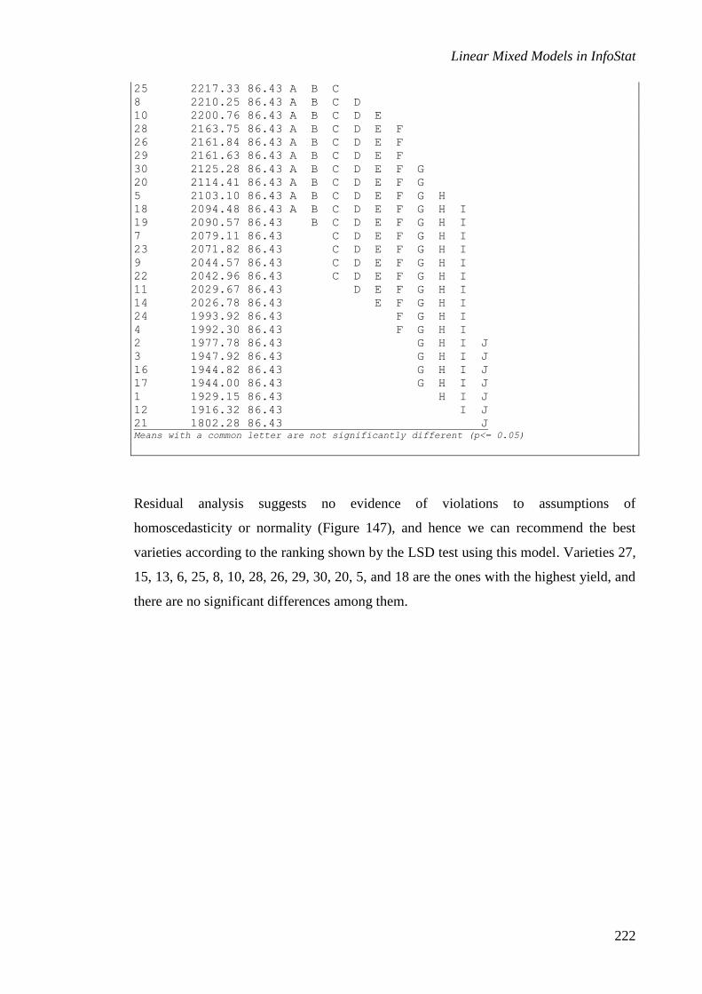
Linear Mixed Models in InfoStat
222
25 2217.33 86.43 A B C
8 2210.25 86.43 A B C D
10 2200.76 86.43 A B C D E
28 2163.75 86.43 A B C D E F
26 2161.84 86.43 A B C D E F
29 2161.63 86.43 A B C D E F
30 2125.28 86.43 A B C D E F G
20 2114.41 86.43 A B C D E F G
5 2103.10 86.43 A B C D E F G H
18 2094.48 86.43 A B C D E F G H I
19 2090.57 86.43 B C D E F G H I
7 2079.11 86.43 C D E F G H I
23 2071.82 86.43 C D E F G H I
9 2044.57 86.43 C D E F G H I
22 2042.96 86.43 C D E F G H I
11 2029.67 86.43 D E F G H I
14 2026.78 86.43 E F G H I
24 1993.92 86.43 F G H I
4 1992.30 86.43 F G H I
2 1977.78 86.43 G H I J
3 1947.92 86.43 G H I J
16 1944.82 86.43 G H I J
17 1944.00 86.43 G H I J
1 1929.15 86.43 H I J
12 1916.32 86.43 I J
21 1802.28 86.43 J Means with a common letter are not significantly different (p<= 0.05)
Residual analysis suggests no evidence of violations to assumptions of
homoscedasticity or normality (Figure 147), and hence we can recommend the best
varieties according to the ranking shown by the LSD test using this model. Varieties 27,
15, 13, 6, 25, 8, 10, 28, 26, 29, 30, 20, 5, and 18 are the ones with the highest yield, and
there are no significant differences among them.
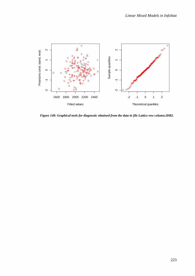
Linear Mixed Models in InfoStat
223
Figure 148: Graphical tools for diagnostic obtained from the data in file Lattice row column.IDB2.
1600 1800 2000 2200 2400
-2-1
01
2
Fitted values
Pe
ars
on
s c
on
d. sta
nd
. re
sd
.
-2 -1 0 1 2
-2-1
01
2
Theoretical quantiles
Sa
mp
le q
ua
ntile
s

Linear Mixed Models in InfoStat
224
Balanced squared lattice design
This example shows data from a trial with 25-wheat variety in 6 repetitions. Rows and
columns effects will be accounted for within each square (repetition). Rows and
columns constitute incomplete blocks. This trial was conducted in 1976 in Slate Hall
Farm, Cambridgeshire, UK (Gleason, 1997). Figure 149 shows the field arrangement.
The data are in the file Square lattice.IDB2. In order to analyze these data we first use
the variable selector window in Extended and mixed linear models. Yield is selected as
variable, and Replication, Row, and Column as class variables (Figure 150). Then we
select Variety in the Fixed effects tab (Figure 151). The Random effects tab is completed
as follows: first we include Repetition, and then we need to indicate that both Row and
Column are nested within Repetition (Figure 152).
1 2 4 3 5 19 23 2 6 15 18 25 9 11 2
6 7 9 8 10 8 12 16 25 4 5 7 16 23 14
21 22 24 23 25 11 20 24 3 7 6 13 22 4 20
11 12 14 13 15 22 1 10 14 18 24 1 15 17 8
16 17 19 18 9 5 9 13 17 21 12 19 3 10 21
3 18 8 13 23 16 24 10 13 2 10 4 17 11 23
1 16 6 11 21 12 20 1 9 23 12 6 24 18 5
5 20 10 15 25 4 7 18 21 15 19 13 1 25 7
2 17 7 12 22 25 2 14 17 6 21 20 8 2 14
4 19 9 14 24 8 11 22 5 19 3 22 15 9 16
Figure 149: Layout of the design for the 25-variety wheat trial conducted in a square lattice whit six
replications (squared) and numbers of each cell represent the varieties.

Linear Mixed Models in InfoStat
225
Figure 150: Window from the Extended and mixed linear model with the variable selection for data in
file Square lattice.IDB2.

Linear Mixed Models in InfoStat
226
Figure 151: Window from the Extended and mixed linear model with the Fixed effect tab for data in
file Square lattice.IDB2.

Linear Mixed Models in InfoStat
227
Figure 152: Window from the Extended and mixed linear model with the Random effect tab for data in
file Square lattice.IDB2.
Extended and mixed linear models
R specification of the model
model.017_Yield_REML<-lme(Yield~1+Variety
,random=list(Replication=pdIdent(~1)
,Replication=pdIdent(~Row-1)
,Replication=pdIdent(~Column-1))
,method="REML"
,control=lmeControl(msMaxIter=200)
,na.action=na.omit
,data=R.data17
,keep.data=FALSE)
Results for model: model.017_Yield_REML
Dependent variable: Yield

Linear Mixed Models in InfoStat
228
Fit measurements
N AIC BIC logLik Sigma R2_0 R2_1 R2_2 R2_3
150 1703.31 1785.33 -822.65 89.79 0.27 0.38 0.67 0.92 Smaller AIC and BIC is better
Marginal hypothesis testing (Type III SS)
numDF denDF F-value p-value
(Intercept) 1 120 1216.28 <0.0001
Variety 24 120 8.84 <0.0001
Sequential hypothesis testing
numDF denDF F-value p-value
(Intercept) 1 120 1216.28 <0.0001
Variety 24 120 8.84 <0.0001
Random effects parameters
Covariance model for random effects: pdIdent
Formula: ~1|Replication
Standard deviations and correlations
(const)
(const) 65.29
Covariance model for random effects: pdIdent
Formula: ~Row - 1|Replication
Standard deviations and correlations
S.D.
1 124.88
2 124.88
3 124.88
4 124.88
5 124.88
Covariance model for random effects: pdIdent
Formula: ~Column - 1|Replication
Standard deviations and correlations
S.D.
1 121.70
2 121.70
3 121.70
4 121.70
5 121.70
Adjusted means and standard error for Variety
LSD Fisher (Alpha:=0.05)
p-value correction procedure: No
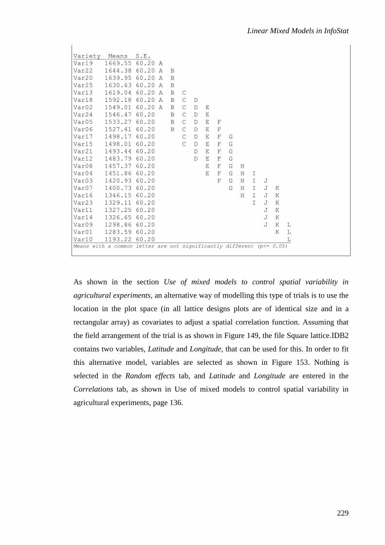
Linear Mixed Models in InfoStat
229
Variety Means S.E.
Var19 1669.55 60.20 A
Var22 1644.38 60.20 A B
Var20 1639.95 60.20 A B
Var25 1630.63 60.20 A B
Var13 1619.04 60.20 A B C
Var18 1592.18 60.20 A B C D
Var02 1549.01 60.20 A B C D E
Var24 1546.47 60.20 B C D E
Var05 1533.27 60.20 B C D E F
Var06 1527.41 60.20 B C D E F
Var17 1498.17 60.20 C D E F G
Var15 1498.01 60.20 C D E F G
Var21 1493.44 60.20 D E F G
Var12 1483.79 60.20 D E F G
Var08 1457.37 60.20 E F G H
Var04 1451.86 60.20 E F G H I
Var03 1420.93 60.20 F G H I J
Var07 1400.73 60.20 G H I J K
Var16 1346.15 60.20 H I J K
Var23 1329.11 60.20 I J K
Var11 1327.25 60.20 J K
Var14 1326.65 60.20 J K
Var09 1298.86 60.20 J K L
Var01 1283.59 60.20 K L
Var10 1193.22 60.20 L Means with a common letter are not significantly different (p<= 0.05)
As shown in the section Use of mixed models to control spatial variability in
agricultural experiments, an alternative way of modelling this type of trials is to use the
location in the plot space (in all lattice designs plots are of identical size and in a
rectangular array) as covariates to adjust a spatial correlation function. Assuming that
the field arrangement of the trial is as shown in Figure 149, the file Square lattice.IDB2
contains two variables, Latitude and Longitude, that can be used for this. In order to fit
this alternative model, variables are selected as shown in Figure 153. Nothing is
selected in the Random effects tab, and Latitude and Longitude are entered in the
Correlations tab, as shown in Use of mixed models to control spatial variability in
agricultural experiments, page 136.
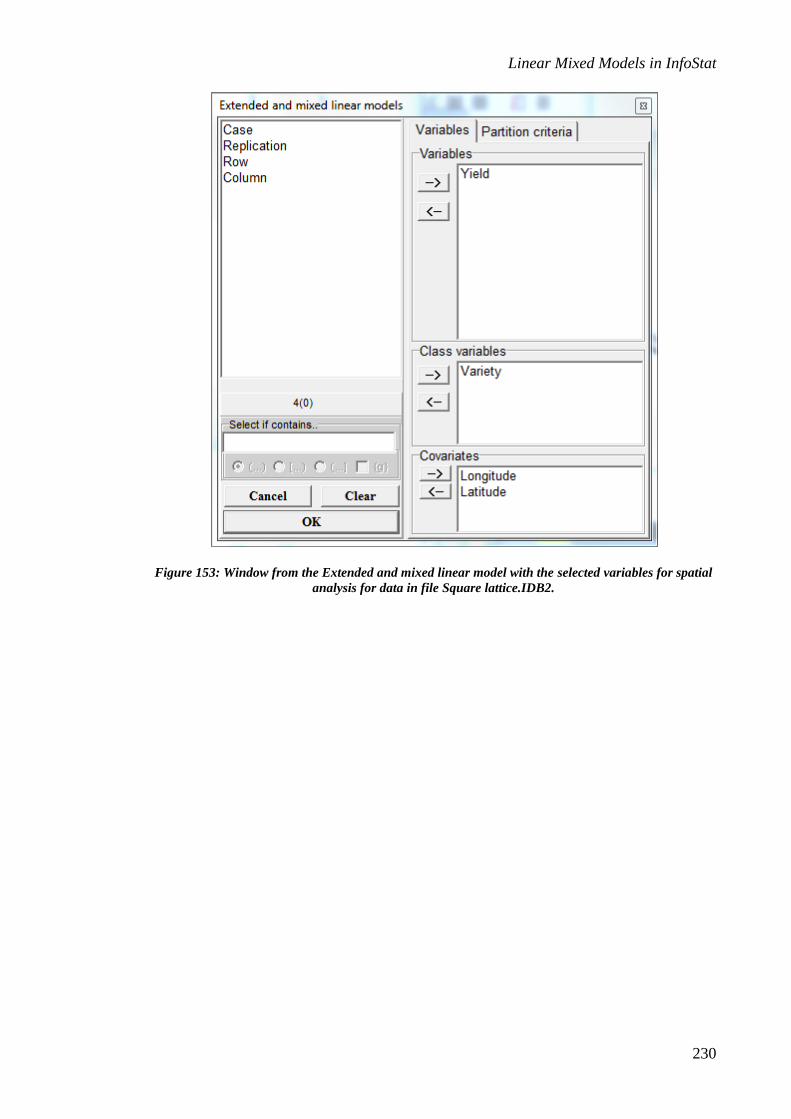
Linear Mixed Models in InfoStat
230
Figure 153: Window from the Extended and mixed linear model with the selected variables for spatial
analysis for data in file Square lattice.IDB2.

Linear Mixed Models in InfoStat
231
Figure 154: Window from the Extended and mixed linear model with the Correlation tab and the
inclusion of Latitude and Longitude for data in file Square lattice.IDB2.
Extended and mixed linear models
R specification of the model
model.018_Yield_REML<-gls(Yield~1+Variety
,correlation=corExp(form=~as.numeric(as.character(Longitude))+as.numer
ic(as.character(Latitude))
,metric="euclidean"
,nugget=FALSE)
,method="REML"
,na.action=na.omit
,data=R.data18)
Results for model: model.018_Yield_REML
Dependent variable: Yield
Fit measurements

Linear Mixed Models in InfoStat
232
N AIC BIC logLik Sigma R2_0
150 1692.55 1768.92 -819.28 212.96 0.27 Smaller AIC and BIC is better
Marginal hypothesis testing (Type III SS)
numDF F-value p-value
(Intercept) 1 399.80 <0.0001
Variety 24 7.70 <0.0001
Sequential hypothesis testing
numDF F-value p-value
(Intercept) 1 393.70 <0.0001
Variety 24 7.70 <0.0001
Correlation structure
Correlation model: Exponential spatial correlation
Formula: ~ as.numeric(as.character(Longitude)) +
as.numeric(as.character(Latitude))
Metric: euclidean
Model parameters
Parameter Estim.
range 2.45
Adjusted means and standard error for Variety
LSD Fisher (Alpha:=0.05)
p-value correction procedure: No
Variety Means S.E.
Var19 1664.57 86.82 A
Var20 1659.01 87.25 A
Var13 1626.37 87.32 A B
Var22 1589.59 87.21 A B C
Var06 1552.97 86.99 A B C D
Var24 1550.00 87.19 A B C D
Var25 1544.63 87.50 A B C D
Var18 1537.52 87.20 A B C D E
Var17 1535.60 87.60 A B C D E
Var02 1531.18 86.48 A B C D E
Var21 1510.73 87.08 B C D E F
Var05 1477.87 86.64 C D E F
Var08 1473.21 87.17 C D E F
Var12 1456.69 87.40 C D E F G
Var15 1422.74 87.02 D E F G H
Var03 1407.62 86.78 E F G H
Var04 1399.11 86.90 E F G H
Var07 1389.06 87.46 F G H
Var16 1332.43 86.72 G H I
Var14 1327.22 87.19 G H I
Var11 1326.39 87.04 G H I
Var23 1306.36 87.02 H I
Var09 1289.71 86.66 H I
Var01 1231.80 86.54 I
Var10 1201.09 87.28 I Means with a common letter are not significantly different (p<= 0.05)

Linear Mixed Models in InfoStat
233
In order to compare the fit of both models, we can compare their AICs or BICs (since
one of the models is not a special case of the other, we cannot conduct a likelihood ratio
test to compare them). The following are the values of AIC and BIC:
Model AIC BIC
IBD 1703.31 1785.33
Spatial correlation 1692.55 1768.92
From these results, the spatial correlation model fits the data better. Nevertheless, if we
compute the average standard errors of the difference of means for both models we find
that the spatial correlation model yields a value of 69.118, while the model considering
the design structure yields a value of 62.019. Hence if the goal is to compare variety
means, the model considering the design structure is more appropriate.

Linear Mixed Models in InfoStat
234
References
Benjamini Y., Hochberg Y.1995. Controlling the false discovery rate: a practical and
powerful approach to multiple testing. J. R. Stat. Soc. Ser. B, 57:289-300.
Benjamini Y., Yekutieli, D. 2001. The control of the false discovery rate in multiple
hypothesis testing under dependency. The Annals of Statistics, 29(4):1165-
1188.
Besag J.E. 1974. Spatial interaction and the statistical analysis of lattice systems. J. R.
Stat. Soc. Ser. B 36: 192-225.
Besag J.E. 1977. Errors-in-variables estimation for Gaussian lattice schemes. J. R. Stat.
Soc. Ser. B 39: 73-78.
Cáceres L., Macchiavelli R, Rojas Y. (2011). A Professional Development Model:
including coaching and problem-based learning. Abstracts, INTED2011
(International Technology, Education and Development Conference),
Valencia, Spain.
Casanoves F., Macchiavelli R., Balzarini, M. 2005. Error variation in multienvironment
peanut trials: Within-trial spatial correlation and between-trial heterogeneity.
Crop Science, 45: 1927-1933.
Casanoves F., Macchiavelli R., Balzarini M. 2007. Models for multi-environment yield
trials with fixed and random block effects and homogeneous and
heterogeneous residual variances. Journal of Agriculture of the University of
Puerto Rico, 91(3-4): 117-131.
Cullis B.R., Gogel B.J., Verbyla A.P., Thompson R. 1998. Spatial analysis of multi-
environment early generation trials. Biometrics 54: 1-18.
Di Rienzo J.A., Guzman A.W., Casanoves F. (2002). A Multiple Comparisons Method
based On the Distribution of the Root Node Distance of a Binary Tree
Obtained by Average Linkage of the Matrix of Euclidean Distances between
Treatment Means. JABES 7(2), 129-142.
Di Rienzo J. 2007.Curso de Diseño de Experimentos 2007 de la Maestría en Estadística
Aplicada – UNC. http://vaca.agro.uncor.edu/~estad/cursosposgrado.htm

Linear Mixed Models in InfoStat
235
Gilmour A.R., Thompson R, Cullis B.R., Verbyla A.P. 1997. Accounting for natural
and extraneous variation in the analysis of field experiments. J. Agric. Biol.
Env. Stat. 2: 269:273.
Gleson A.C. 1997. Spatial Analysis. In R.A. Kempton, P.N. Fox (eds) Statistical
Methods for Plant Variety Evaluation. Chapman & Hall, London.
Hsu J.C. 1996. Multiple Comparisons: Theory and Methods. First edition. Chapman &
Hall, London.
Littell R., Milliken G., Stroup W., Wolfinger R., Schabenberger O. 2006. SAS for
Mixed Models. Second Ed., SAS Institute, Cary, NC.
Littell R., Pendergast J., Natarajan R. 2002. Modelling Covariance Structure in the
Analysis of Repeated Measures Data. Statistics in Medicine 19:1793-1819.
Martínez N. 2006. Determinación de la tasa de degradación de hojarasca de guadua
(Guadua angustifolia) e higuerón (Ficus glabrata) con y sin presencia de
macroinvertebrados acuáticos en una quebrada del Valle del Cauca, Colombia.
Disertación, Departamento de Biología, Universidad del Valle, Colombia.
Mead R. 1971. Models for interplant competition in irregularly spaced population. In:
Statistical Ecology, Patil G.P., Pielou E.C. and Waters W.E. (Eds.).
Pensilvania State University Press, State College, PA, pp: 13-22.
Milliken G.A., Johnson D.E. 1992. Analysis of Messy Data, Vol. 1. Chapman and Hall:
Londres.
Moser E.B., Macchiavelli R. 2002. Model selection techniques for repeated measures
covariance structures. Proceedings of the XIV Conference on Applied
Statistics in Agriculture 14: 17-31.
Navarro C., Cavers S., Pappinen A., Tigerstedt P., Lowe A., Merila J. 2005. Contrasting
quantitative traits and neutral genetic markers for genetic resource assessment
of Mesoamerican Cedrela odorata. Silvae Genetica. 54: 281–292.
Ospina S. 2010. Linking plant strategies and ecosystem function: an assessment of the
contribution of biodiversity to Neotropical grassland productivity. Ph.D. Tesis.
School of the Environment, Natural Resources and Geography, Bangor
University, Gwynedd, United Kingdom, and Program Tropical Agricultural
Research and Higher Education Center (CATIE). Bangor, Reino Unido. 163 p.
Linear Mixed Models in InfoStat
236
Ospina S., Rusch G.M., Pezo D., Casanoves F., Sinclair F.L. 2012. More stable
productivity of semi natural grasslands than sown pastures in a seasonally dry
climate. Sent to PLoS ONE.
Papadakis J.S. 1937. Méthode statistique pour des experiences sur champ. Institut
d’Amélioration des Plantes a Thessaloniki.
Patterson H.D.,Thompson R., Hunter E.R., Williams E.R. 1989. Analysis of non-
orthogonal data using REML. Scottish Agricultural Statistical Services
(unpublished notes from an internal course).
Pinheiro J.C., Bates D.M. 2004. Mixed-Effects Models in S and S-PLUS. Springer,
New York.
Pierson R.A., Ginther O.J. 1987. Follicular population dynamics during the estrus cycle
of the mare. Animal Reproduction Science 14: 219–231.
Ripley B.D. 1981. Spatial Statistics. Wiley, New York.
Williams E.R. 1986. Row and column designs with contigous replicates. Australian
Journal of Statistics 28 :149-154.
Zimmerman D.L., Harville D.A. 1991. A random field approach to the analysis of field
plot experiments and other spatial experiments. Biometrics 47: 223-239.

Linear Mixed Effects Models in InfoStat
237
Table index
Table 1. Estimated variance components (VarCom.IDB2 file) .................................................................................... 39
Table 2. Characteristics and fitted measures of the evaluated model (Respiratory capacity.IDB2 file)...................... 115
Table 3. Goodness of fit criteria for the adjusted models with a fixed block effect (Peanut MET.IDB2 file). ........... 151
Table 4. Goodness of fit criteria for the adjusted models without a fixed block effect (Peanut MET.IDB2 file). ...... 151
Figures index
Figure 1: Tabs with the options for the specification of an extended and mixed linear model. ......................................2
Figure 2: Window displaying the Fixed effects tab (Atriplex.IDB2 file)........................................................................3
Figure 3: Window displaying the Random effects tab (Block.IDB2 file). ......................................................................5
Figure 4: Window displaying the Comparisons tab (Block.IDB2 file). ..........................................................................8
Figure 5: Window with the Random effects tab for a hypothetical example with four classification factors: A, B, C,
and D (A is fixed; B, C, and D are random). In this case B, C, and D are included as nested random effects. ...............9
Figure 6: Window with the Random effects tab for a hypothetical example with four classification factors: A, B, C,
and D (A is fixed; B, C, and D are random). In this case B, C, and D are included as nested random effects (explicit
form). ............................................................................................................................................................................ 10
Figure 7: Window with the Random effects tab for a hypothetical example with four classification factors: A, B, C,
and D (A is fixed; B, C, and D are random.) In this case D and C are included as crossed random effects................. 10
Figure 8: Window with the Random effects tab for a hypothetical example with four classification factors: A, B, C,
and D (A is fixed; B, C, and D are random.) In this case D and C are included as crossed random effects with
interaction. .................................................................................................................................................................... 11
Figure 9: Window with the Random effects tab for a hypothetical example with four classification factors: A, B, C,
and D (A is fixed; B, C, and D are random.) In this case D and C are included as crossed random effects with
interaction, and B is nested in C. .................................................................................................................................. 11
Figure 10: Window with the Random effects tab for a hypothetical example with four classification factors: A, B, C,
and D (A is fixed; B, C, and D are random.) In this case B and C are included as crossed random effects, both nested
within the fixed factor A. .............................................................................................................................................. 11
Figure 11: Window with the Random effects tab for a hypothetical example with four classification factors: A, B, C,
and D (A is fixed; B, C, and D are random.) In this case C are D are included as crossed random effects, both nested
within the random effect B. .......................................................................................................................................... 12
Figure 12: Dialogue window for importing data from R libraries. ............................................................................... 13
Figure 13: Heading of the data table (Ovary file). ........................................................................................................ 14
Figure 14. Relationship between the number of follicles and time. .............................................................................. 14
Figure 15: Window displaying the Fixed effects tab (Ovary file). ................................................................................ 16
Figure 16: Window displaying the Random effects tab (Ovary file). ........................................................................... 17

Linear Mixed Effects Models in InfoStat
238
Figure 17: Window displaying the Correlation tab (Ovary file). .................................................................................. 18
Figure 18: Fitted functions for the population number of follicles (solid black line) and for each mare generated by
the random effect on the constant (Ovary file). ............................................................................................................ 21
Figure 19: Smooth functions (third order polynomial) for the number of follicles (solid black lines) for each mare
generated by the random effect on the constant (Ovary file). ....................................................................................... 22
Figure 20: Specification of the fixed part of model (3) ................................................................................................. 22
Figure 21: Specification of the random part of model (3). Different variances for each random effect........................ 23
Figure 22: Predicted values for the number of follicles of each mare generated by the inclusion of random effects on
all parameters of the fixed part of the model (pdDiag covariance structure) (Ovary file). .......................................... 23
Figure 23: Specification of the random part of model (3), with different variances of each random effect and random
effects correlated .......................................................................................................................................................... 24
Figure 24: Predicted values for the number of follicles of each mare generated by the inclusion of random effects on
all parameters of the fixed part of the model (pdSym covariance structure) (Ovary file). ........................................... 24
Figure 25: Window displaying the Heteroscedasticity tab (Ovary file). ....................................................................... 26
Figure 26: Model exploration window displaying the Diagnostic tab (Atriplex.IDB2 file). ......................................... 29
Figure 27: Model exploration window displaying the Linear combination tab (Atriplex.IDB2 file). ........................... 30
Figure 28: Residual autocorrelation function of the model shown in Equation, excluding serial autocorrelation. ....... 31
Figure 29: Residual autocorrelation function of the model presented in Equation (2), including serial autocorrelation.
...................................................................................................................................................................................... 32
Figure 30: Variables selection window for extended and mixed linear models (VarCom.IDB2 file). .......................... 36
Figure 31: Window displaying the Random effects tab for Model 1(VarCom.IDB2 file). ........................................... 37
Figure 32: Model exploration window displaying the Diagnostic tab for Model 1 (VarCom.IDB2 file). .................... 40
Figure 33: Diagnostic graphs obtained for the variable Length, Model 1 (VarCom.IDB2 file). ................................... 40
Figure 34: Window displaying the Heteroscedasticity tab for the specification of heterogeneous variables for
populations (VarCom.IDB2 file). ................................................................................................................................. 41
Figure 35: Diagnostic graphs obtained for the variable Length, Model 1 with heterogeneous residual variables for
populations (VarCom.IDB2 file). ................................................................................................................................. 46
Figure 36: Window displaying the Fixed effects tab, Model 2 (VarCom.IDB2 file). ................................................... 47
Figure 37: Window displaying the Random effects tab, Model 2 (VarCom.IDB2 file). .............................................. 47
Figure 38: Window displaying the Comparisons tab, Model 2 (VarCom.IDB2 file).. .................................................. 48
Figure 39: Model exploration window displaying the Diagnostic tab, Model 2 (VarCom.IDB2 file). ......................... 52
Figure 40: Diagnostic graphs obtained for the variable Length, Model 2 (VarCom.IDB2 file). ................................... 53
Figure 41: Diagnostic graphs obtained for the variable Length once the different residual variances for each
population were declared, Model 2 (VarCom.IDB2 file). ............................................................................................ 56

Linear Mixed Effects Models in InfoStat
239
Figure 42: Window displaying the Random effects tab with Line and Operator effects crossed and their interaction,
file Production.IDB2. ................................................................................................................................................... 58
Figure 43: Scheme of the split plots design for the example (Wheat.IDB2 file, light gray =irrigation, dark
gray=rainfed). ............................................................................................................................................................... 63
Figure 44: Heading of the data table (Wheat.IDB2 file). .............................................................................................. 63
Figure 45: Variables selection window for Extended and mixed linear models (Wheat.IDB2 file). ............................ 64
Figure 46: Window displaying the Fixed effects tab (Wheat.IDB2 file). ..................................................................... 65
Figure 47: Window displaying the Random effects tab, with Block and Water as stratification criteria (Wheat.IDB2
file). .............................................................................................................................................................................. 66
Figure 48: Model exploration window for the comparison of extended and mixed models displaying the Diagnostic
tab (Wheat.IDB2 file). .................................................................................................................................................. 68
Figure 49: Diagnostic graphs (Wheat.IDB2 file). ......................................................................................................... 69
Figure 50: Window displaying the Heteroscedasticity tab, with the varIdent function with Variety selected as a
grouping variable (Wheat.IDB2 file). ........................................................................................................................... 70
Figure 51: Window displaying the Comparisons tab, and the selection of the Means subtab (Wheat.IDB2 file). ........ 71
Figure 52: Heading of the data table (Coverage drops.IDB2 file). ............................................................................... 73
Figure 53: Variables selection window for Extended and mixed linear models (Coverage drops.IDB2 file). .............. 74
Figure 54: Window displaying the Fixed effects tab (Coverage drops.IDB2 file). ....................................................... 74
Figure 55: Window displaying the Random effects tab, with Plot as the stratification criterion (Coverage drops.IDB2
file). .............................................................................................................................................................................. 75
Figure 56: Box plots for the Pearson standardized residuals for the levels of the factor Face. ..................................... 77
Figure 57: Window displaying the Heteroscedasticity tab, with Face as a grouping variable (Coverage drops.IDB2
file). .............................................................................................................................................................................. 78
Figure 58: Dot plot for the study of the interaction between Adjuvant and Height (a) and between Face and Height
(b). ................................................................................................................................................................................ 81
Figure 59: Diagram of the split-split plot design for the example (Starch quality.IDB2 file). ...................................... 82
Figure 60: Heading of the data table (Starch quality.IDB2). ........................................................................................ 82
Figure 61: Variables selection window for the Extended and mixed linear models (Starch quality.IDB2 file). ........... 83
Figure 62: Window with the tab Fixed effects displayed for the data in the file Starch quality.IDB2. ......................... 84
Figure 63: Window displaying the Random effects tab (Starch quality.IDB2 file). ..................................................... 85
Figure 64: Window displaying the Random effects tab that shows another way to specify the random part (Starch
quality.IDB2 file).......................................................................................................................................................... 87
Figure 65: Relationship between Coverage and Time for five treatments (Forage Coverage.IDB2 file). .................... 91
Figure 66: Variables selection window for Extended and mixed linear models (Forage Coverage.IDB2 file)............. 93
Figure 67: Window displaying the Fixed effects tab (Forage Coverage.IDB2 file). ..................................................... 94

Linear Mixed Effects Models in InfoStat
240
Figure 68: Window displaying the Random effect tab for model 1(Forage Coverage.IDB2 file). ............................... 95
Figure 69: Window displaying the Correlation tab and the selection of Independent errors (Model 1) (Forage
Coverage.IDB2 file). .................................................................................................................................................... 96
Figure 70: Window displaying the Random Effect tab, with Block and Plot selected (Model 2) (Forage
Coverage.IDB2 file). .................................................................................................................................................... 97
Figure 71: Window displaying the Heteroscedasticity tab, with the varIdent function selected and Time as the
grouping variable (Model 2) (Forage Coverage.IDB2 file). ......................................................................................... 98
Figure 72: Window displaying the Correlation tab, and selection of Compound symmetry for data grouped block and
plot (Forage Coverage.IDB2 file). ................................................................................................................................ 99
Figure 73: Window displaying the Correlation tab, and selection of the Autoregressive of order 1. Data grouped by
Block and Plot, and the order of the observations indicated by the variable Time (Forage Coverage.IDB2 file). ...... 101
Figure 74: Window displaying the Correlation tab, and the selection of the General positive symmetric matrix Model
for the data grouped by plot, and the order of the observations indicated by the variable Time (Forage Coverage.IDB2
file). ............................................................................................................................................................................ 103
Figure 75: InfoStat Probability and quantile calculator window. ................................................................................ 106
Figure 76: Window displaying the Comparisons tab, with the Contrasts subtab selected (Forage Coverage.IDB2 file).
.................................................................................................................................................................................... 107
Figure 77: Variable selector window (Respiratory capacity.IDB2 file). ..................................................................... 110
Figure 78: Window displaying the Fixed effects tab (Respiratory capacity.IDB2 file). ............................................. 111
Figure 79: Window displaying the Correlation tab, with the Compound symmetry option selected (Respiratory
capacity.IDB2 file). .................................................................................................................................................... 112
Figure 80: Window displaying the Correlation tab, with the Autoregressive of order 1 option selected (Respiratory
capacity.IDB2 file). .................................................................................................................................................... 113
Figure 81: Window displaying the Heteroscedasticity tab (Respiratory capacity.IDB2 file)...................................... 113
Figure 82: Window displaying the Random effects tab (Respiratory capacity.IDB2 file). ......................................... 114
Figure 83: Window displaying the Correlation tab, with the General positive symmetric matrix option selected
(Respiratory capacity.IDB2 file). ................................................................................................................................ 114
Figure 84: Variables selector window (Respiratory capacity average.IDB2 file). ...................................................... 119
Figure 85: Variables selector window displaying the activated Partitions tab (Respiratory capacity average.IDB2 file).
.................................................................................................................................................................................... 119
Figure 86: Box plot to study the interactions between treatments and time with the data from the Respiratory
capacity.IDB2 file. ...................................................................................................................................................... 120
Figure 87: Window displaying the Comparisons tab, Contrasts subtab (Respiratory capacity.IDB2 file). ................. 121
Figure 88: Dot plot for the logarithm of remnant dry weight as a function of Time for the four treatments (Species-
Bag) (Decomposition.IDB2 file). ............................................................................................................................... 124

Linear Mixed Effects Models in InfoStat
241
Figure 89: Specification of the linear regression model with different intercepts and slopes for the logarithm of
remnant dry matter as a function of Time for the four treatments determined by the combination of species and bag
type (Species-Bag) (Decomposition.IDB2 file). ......................................................................................................... 125
Figure 90: Dot plot for the Predicted value (logarithm of remnant dry weight) as a function of Time for the four
treatments (Species-Bag) (Decomposition.IDB2 file). ............................................................................................... 125
Figure 91: Graph of Pearson studentized residuals vs. Time for a regression model of remnant dry matter as a
function of Time for the four treatments (Species-Bag) with different intercepts and slopes, (Decomposition.IDB2
file). ............................................................................................................................................................................ 126
Figure 92: Specification of the linear regression model with different intercepts and slopes for the logarithm of
remnant dry matter as a function of Time for the four Species-Bag treatments (Descomposition.IDB file2). ........... 127
Figure 93: Fits for the second-order polynomial regression model with different intercepts and slopes for the
logarithm of remnant dry matter as a function of Time^2 (centered) for four Species-Bag treatments
(Decomposition.IDB2 file). ........................................................................................................................................ 127
Figure 94: Studentized residuals (Pearson) vs. Time for the second-order polynomial regression model with different
intercept and slopes for the logarithm of remnant dry weight as a function of Time and Time^2 (centered) for four
Species-Bag treatments (Decomposition.IDB2 file). .................................................................................................. 128
Figure 95: Specification of the heteroscedastic part of the second-order polynomial regression model with different
intercepts and slopes for the logarithm of remnant dry weight as a function of Time and Time^2 (centered) for four
Species-Bag treatments (Decomposition.IDB2 file). .................................................................................................. 129
Figure 96: Studentized residuals (Pearson) vs. Time for the heteroscedastic regression model with different intercepts
and slopes by treatment for the logarithm of Remnant dry weight as a function of Time and Time^2 (centered) for the
four treatments (Species-Bag) (Decomposition.IDB2 file). .......................................... ¡Error! Marcador no definido.
Figure 97: Specification of the random part of the second-order heteroscedastic regression model with different
intercepts and slopes for the logarithm of Remnant dry weight as a function of Time and Time^2 (centered) for the
four treatments (Species-Bag) (Decomposition.IDB2 file). ........................................................................................ 130
Figure 98: Studentized residuals (Pearson) vs. Time for the heteroscedastic regression model with different intercept
and slopes by treatment and the addition of a random effect on the constant that is particular for each combination of
Time and Treatment, for the logarithm of remnant dry weight as a function of Time and Time^2 (centered) for the
four treatments (Species-Bag) (Decomposition.IDB2 file). ........................................................................................ 131
Figure 99: R interface with four panels: Script contains the R programs to be executed, Output shows the executed
script, Objects shows the list of objects retained in R’s memory, and the bottom panel shows messages and error
reports sent by R to the console. ................................................................................................................................. 132
Figure 100: Decomposition curves, by species and bag type. ..................................................................................... 135
Figure 101: Window displaying the Fixed effects tab, FB Model (Peanut MET.IDB2 file). ...................................... 139
Figure 102: Window displaying the Fixed effects tab, RB Model (Peanut MET.IDB2 file). ..................................... 140
Figure 103: Window displaying the Random effects tab, RB Model (Peanut MET.IDB2 file). ................................. 140
Figure 104: Window displaying the Heteroscedasticity tab, with Location as the grouping variable, FBE and RBE
models (Peanut MET.IDB2 file). ................................................................................................................................ 141

Linear Mixed Effects Models in InfoStat
242
Figure 105: Window displaying the Correlation tab using the la and lon variables as X and Y coordinates,
respectively, and Site as the grouping variable, Exp and FBExp Models (Peanut MET.IDB2 file). .......................... 142
Figure 106: Dot plot used to study the interaction between Location and Genotype for the variable Yield (Peanut
MET.IDB). ................................................................................................................................................................. 156
Figure 107: Outline of an experiment conducted under a strip-plot design, repeated in completely randomized blocks
with the randomization of the factors Nitrogen and Amount of irrigation for a particular block (StripPlot.IDB2 file).
.................................................................................................................................................................................... 158
Figure 108: Dot plot used to explore the means of Irrigation and Nitrogen (StripPlot.IDB2 file). ............................. 159
Figure 109: Window displaying the Fixed effects tab to evaluate a mixed model (StripPlot.IDB2 file). ................... 160
Figure 110: Window displaying the Random effects tab to evaluate a mixed model (StripPlot.IDB2 file). .............. 161
Figure 111: Window displaying the Random effects tab to evaluate a mixed model with Nitrogen and Irrigation as
cross factors (StripPlot.IDB2 file). ............................................................................................................................. 163
Figure 112: Variables selector window for the Extended and mixed linear model (Earthworms.IDB2 file). ............. 166
Figure 113: Window displaying the Fixed effects tab for evaluating a mixed model (Earthworms.IDB2 file). ......... 167
Figure 114: Window displaying the Correlation tab for evaluating a mixed model with exponential spatial correlation
(Earthworms.IDB2 file). ............................................................................................................................................. 168
Figure 115: Window displaying the Correlation tab for evaluating a mixed model with first-order autoregressive
correlation (Earthworms.IDB2 file). ........................................................................................................................... 170
Figure 116: Graphic diagnostic tools (Earthworms.IDB2 file). .................................................................................. 172
Figure 117: Window displaying the Heteroscedasticity tab for evaluating a mixed model (Earthworms.IDB2 file). 173
Figure 118: Dot plot used to study the interaction between Treatments and Depth and its effect on biomass
(Earthworms.IDB2 file). ............................................................................................................................................. 175
Figure 119: Window displaying the Comparisons tab and Contrasts subtab for evaluating a mixed model
(Earthworms.IDB2 file). ............................................................................................................................................. 176
Figure 120: Window displaying the Fixed effects tab (Matched checks.IDB2 file). .................................................. 179
Figure 121: Window displaying the Correlation tab, and selection of Exponential spatial correlation (Matched
checks.IDB2 file). ....................................................................................................................................................... 181
Figure 122: Window displaying the Correlation tab, and selection of Guassian spatial correlation (Matched
checks.IDB2 file). ....................................................................................................................................................... 182
Figure 123: Window displaying the Correlation tab, and selection of Linear spatial correlation (Matched checks.IDB2
file). ............................................................................................................................................................................ 183
Figure 124: Window displaying the Correlation tab, and selection of “Rational quadratic” spatial correlation
(Matched checks.IDB2 file). ....................................................................................................................................... 184
Figure 125: Window displaying the Correlation tab, and selection of Spherical spatial correlation (Matched
checks.IDB2 file). ....................................................................................................................................................... 185
Figure 126: Variables selector window for the Extended and mixed linear models (Matched checks.IDB2 file). ..... 188

Linear Mixed Effects Models in InfoStat
243
Figure 127: Relationship between Learning gain and Pre-test score, smoothed separately for each teacher. File
Learning.idb2.............................................................................................................................................................. 190
Figure 128: Window to select fixed effects in the Extended and mixed models for the data in the file LearningIDB2.
.................................................................................................................................................................................... 191
Figure 129: Extended and mixed linear models with the Random effects tab for the data in the file Learning.IDB2.
.................................................................................................................................................................................... 192
Figure 130: Variable selection window in the Extended and mixed linear models module for the data in file Primary
productivity.IDB2. ...................................................................................................................................................... 194
Figure 131: Window from the Extended and mixed linear model with the Fixed effects tab for the data in file Primary
productivity.IDB2. ...................................................................................................................................................... 195
Figure 132: Window from the Extended and mixed linear model with the Random effects tab for the data in file
Primary productivity.IDB2. ........................................................................................................................................ 196
Figure 133: Graphical tools for diagnostic obtained from the data in file Primary productivity.IDB2 with Rain as
regressor and Pasture as fixed factor. ......................................................................................................................... 197
Figure 134: Graphical tools for diagnostic obtained from the data in file Primary productivity.IDB2 with Rain and
POW_Rain as regressors and Pasture as fixed factor. ................................................................................................ 198
Figure 135: Window from the Extended and mixed linear model with the Heteroscedasticity tab for the data in file
Primary productivity.IDB2, and the selection of the function VarPower. .................................................................. 199
Figure 136: Graphical tools for diagnostic obtained from the data in file Primary productivity.IDB2 with Rain and
POW.Rain as regressors, Pasture as fixed factor, and a VarPower function to model variance heterogeneity. .......... 200
Figure 137: Window from the Extended and mixed linear model for the data in file Primary productivity.IDB2, and
the specification of the model with interaction. .......................................................................................................... 201
Figure 138: Window from the Extended and mixed linear model module with the Random effects tab for the data in
file Primary productivity.IDB2. .................................................................................................................................. 202
Figure 139: Scatterplot showing the relationship between primary productivity and rain for each of the two pastures.
File Primary productivity.IDB2. ................................................................................................................................. 206
Figure 140: Model exploration window with Linear combination tab for the data in file Primary productivity.IDB2.
.................................................................................................................................................................................... 207
Figure 141: Layout of the design for the 18-variety barley trial conducted in an alpha-lattice. Roman numbers at the
right indicate replicates, arabic numbers at the top of each cell indicate the incomplete block (of sizes 4 and 3), and
numbers at the bottom of each cell represent the varieties. ......................................................................................... 208
Figure 142: Window from the Extended and mixed linear model with the Fixed effects tab for the data in file Alpha
lattice.IDB2. ............................................................................................................................................................... 209
Figure 143: Window from the Extended and mixed linear model with the Random effects tab and the Replication
effect for the data in file Alpha lattice.IDB2............................................................................................................... 210
Figure 144: Window from the Extended and mixed linear model with the Random effects tab and the Replication and
Incomplete block effect for the data in file Alpha lattice.IDB2. ................................................................................. 212

Linear Mixed Effects Models in InfoStat
244
Figure 145: Field layout for a 30-variety cotton trial conducted as a latinized row-column design with five replication.
.................................................................................................................................................................................... 217
Figure 146: Window from the Extended and mixed linear model with the Fixed effects tab and the Variety effect for
the data in file Lattice row column.IDB2. .................................................................................................................. 218
Figure 147: Window from the Extended and mixed linear model with the Random effects tab and the Column, Row
and Replication effects for the data in file Lattice row column.IDB2. ....................................................................... 219
Figure 148: Graphical tools for diagnostic obtained from the data in file Lattice row column.IDB2. ........................ 223
Figure 149: Layout of the design for the 25-variety wheat trial conducted in a square lattice whit six replications
(squared) and numbers of each cell represent the varieties. ........................................................................................ 224
Figure 150: Window from the Extended and mixed linear model with the variable selection for data in file Square
lattice.IDB2. ............................................................................................................................................................... 225
Figure 151: Window from the Extended and mixed linear model with the Fixed effect tab for data in file Square
lattice.IDB2. ............................................................................................................................................................... 226
Figure 152: Window from the Extended and mixed linear model with the Random effect tab for data in file Square
lattice.IDB2. ............................................................................................................................................................... 227
Figure 153: Window from the Extended and mixed linear model with the selected variables for spatial analysis for
data in file Square lattice.IDB2. .................................................................................................................................. 230
Figure 154: Window from the Extended and mixed linear model with the Correlation tab and the inclusion of
Latitude and Longitude for data in file Square lattice.IDB2. ...................................................................................... 231