linear elliptic equations of second ordermiersemann/pde2book.pdflinear elliptic equations of second...
TRANSCRIPT

Linear Elliptic Equations of Second Order
Lecture Notes
Erich MiersemannDepartment of Mathematics
Leipzig University
Version October, 2012

2

Contents
1 Potential theory 71.1 Preliminaries . . . . . . . . . . . . . . . . . . . . . . . . . . . 91.2 Dipole potential . . . . . . . . . . . . . . . . . . . . . . . . . . 111.3 Single layer potential . . . . . . . . . . . . . . . . . . . . . . . 201.4 Integral equations . . . . . . . . . . . . . . . . . . . . . . . . 261.5 Volume potential . . . . . . . . . . . . . . . . . . . . . . . . . 381.6 Exercises . . . . . . . . . . . . . . . . . . . . . . . . . . . . . 43
2 Perron’s method 472.1 A maximum principle . . . . . . . . . . . . . . . . . . . . . . 472.2 Subharmonic, superharmonic functions . . . . . . . . . . . . . 502.3 Boundary behaviour . . . . . . . . . . . . . . . . . . . . . . . 56
2.3.1 Examples for local barriers . . . . . . . . . . . . . . . 592.4 Generalizations . . . . . . . . . . . . . . . . . . . . . . . . . . 632.5 Exercises . . . . . . . . . . . . . . . . . . . . . . . . . . . . . 65
3 Maximum principles 673.1 Basic maximum principles . . . . . . . . . . . . . . . . . . . . 67
3.1.1 Directional derivative boundary value problem . . . . 723.1.2 Behaviour near a corner . . . . . . . . . . . . . . . . . 733.1.3 An apriori estimate . . . . . . . . . . . . . . . . . . . . 76
3.2 A discrete maximum principle . . . . . . . . . . . . . . . . . . 773.3 Exercises . . . . . . . . . . . . . . . . . . . . . . . . . . . . . 83
3

4 CONTENTS

Preface
These lecture notes are intented as an introduction to linear second orderelliptic partial differential equations. It can be considered as a continuationof a chapter on elliptic equations of the lecture notes [17] on partial differen-tial equations. In [17] we focused our attention mainly on explicit solutionsfor standard problems for elliptic, parabolic and hyperbolic equations.
The first chapter concerns integral equation methods for boundary valueproblems of the Laplace equation. This method can be extended to a largeclass of linear elliptic equations and systems. In the following chapter weconsider Perron’s method for the Dirichlet problem for the Laplace equation.This method is based on the maximum principle and on an estimates ofderivatives of solutions of the Laplace equation.
For additional reading we recommend following books: W. I. Smirnov [21],I. G. Petrowski [20], D. Gilbarg and N. S. Trudinger [10], S. G. Michlin [14],P. R. Garabedian [9], W. A. Strauss [22], F. John [13], L. C. Evans [5] andR. Courant and D. Hilbert [4]. Some material of these lecture notes wastaken from some of these books.
5

6 CONTENTS

Chapter 1
Potential theory
The notation potential has its origin in Newton’s attraction rule
K(x, y) = −GMm
|y − x|2y − x
|y − x| ,
where G = 6.67 · 10−11 m3/(kg · s2), and K is the force acting between twomass points M and m located at x, y ∈ R
3, respectively. Since rot K = 0,there is a scalar function Q(x, y), called potential, such that ∇xQ(x, y) =K(x, y). Thus Q(x, y) = −GMm|y − x|−1 is a Newton potential. Thefunction Q(x, y) defines the work which has to be done to move one of themass points to infinity if the other one is fixed.
Let Ω ⊂ Rn be a bounded, connected and sufficiently regular domain.
Consider for given f and h the boundary value problem
−4v = f in Ω
v = h on ∂Ω.
We can transform this problem into a boundary value problem for theLaplace equation by setting v = u − w, where
w(x) =
∫
Ωs(|x − y|)f(y) dy.
Here s(r) denotes the singularity function, see also [17],
s(r) :=
− 12π
ln r : n = 2r2−n
(n−2)ωn: n ≥ 3
We recall that ωn = |∂B1(0)|. Since w ∈ C1(Rn) and −4w = f in Ω iff is sufficiently regular, see Section 5.1, we arrive at the problem 4u = 0
7

8 CHAPTER 1. POTENTIAL THEORY
in Ω and v = h − w on ∂Ω. Consequently, it is sufficient to consider theboundary value problem for the Laplace equation, which is a problem witha homogeneous differential equation.
The Dirichlet problem (first boundary value problem) is to find a solutionu ∈ C2(Ω) ∩ C(Ω) of
4u = 0 in Ω (1.1)
u = Φ on ∂Ω, (1.2)
where Φ is given and continuous on ∂Ω.The Neumann problem (second boundary value problem) is to find a
solution u ∈ C2(Ω) ∩ C1(Ω) of
4u = 0 in Ω (1.3)
∂u
∂n= Ψ on ∂Ω, (1.4)
where Ψ is given and continuous on ∂Ω.In [17], Chapter 7, we derived an explicit formula for the solution of (1.1),
(1.2) if Ω is a ball. In general, one gets explicit solutions, provided the Greenfunction is known for the domain Ω considered.
We denote (1.1), (1.2) by (Di) and (1.3), (1.4) by (Ni) to indicate thatthe problems considered concerns the interior of Ω. Then (De) and (Ne)denote the associated exterior problems, that is we have to replace in (1.1)and (1.3) the domain Ω by its complement R
n \ Ω.
For the Dirichlet problems we make an ansatz with a dipole potential
W (z) =
∫
∂Ωσ(y)
∂
∂ν(y)
(
1
|z − y|n−2
)
dSy (1.5)
if n ≥ 3. In the case that n = 2 we have to replace |z−y|2−n by − ln(|z−y|).In the formula above ν(y) denotes the exterior unit normal at y ∈ ∂Ω andσ(y) the dipole density.
For the Neumann problem we make an ansatz with a single layer potential
V (z) =
∫
∂Ω
σ(y)
|z − y|n−2dSy (1.6)
if n ≥ 3. In the case that n = 2 we have to replace |z−y|2−n by − ln(|z−y|).

1.1. PRELIMINARIES 9
Both potentials solve the Laplace equation in Rn \ ∂Ω.
In the rest of this chapter we assume that n ≥ 3.
We will see that discontinuous properties of these surface potentials leadto integral equations which can be studied by using Fredholm’s results onintegral equations. Thus the method of surface potentials provide a beautifulexample for Fredholm’s theory.
1.1 Preliminaries
Let Ω ⊂ Rn be a bounded and connected domain with a sufficiently regular
boundary ∂Ω.
Definition. We say that ∂Ω ∈ C1,λ, 0 < λ ≤ 1, if:
(i) For each given x ∈ ∂Ω there exists a ρ > 0 and N = N(x, ρ) ballsB2ρ(xi) ⊂ R
n, i = 1, . . . , N , with centers xi ∈ ∂Ω, where x1 = x, such that
∂Ω ⊂N⋃
i=1
Bρ(xi).
(ii) Let Txibe a plane which contains xi and denote by Z2ρ(xi) a circular
cylinder parallel to the normal on Txisuch that its intersection with the
plane Txiis a ball in R
n−1 with radius 2ρ and the center at xi. We assumethe intersection ∂Ω ∩ Z2ρ(xi) has a local representation τ = f(ξ), f ≡ fi,where ξ is in an (n − 1)-dimensional ball D2ρ = D2ρ(0) with radius 2ρ andthe center at 0 ∈ R
n−1. Moreover, we assume
f ∈ C1,λ(D2ρ), f(0) = 0, ∇f(0) = 0.
Lemma 1.1.1 (Partition of unity). There exists ηi ∈ C∞0 (B2ρ(xi)), 0 ≤
ηi ≤ 1, such thatN
∑
i=1
ηi(x) = 1 if x ∈N⋃
i=1
Bρ(xi).
Proof. For given B2ρ(xi) there exists φi ∈ C∞0 (B2ρ(xi)) with the properties

10 CHAPTER 1. POTENTIAL THEORY
T
Z
xi
2
2
ρ
ρ
δΩ
(xi)
xi
B2ρ(xi)
Figure 1.1: Definition of ∂Ω ∈ C1,λ
that φi = 1 in Bρ(xi) and 0 ≤ φi(x) ≤ 1, see an exercise. Set
η1 = φ1
= 1 − (1 − φ1),
ηi = φi(1 − φ1) · . . . · (1 − φi−1)
= (1 − (1 − φi))(1 − φ1) · . . . · (1 − φi−1).
ThenN
∑
i=1
ηi(x) = 1 − (1 − φ1) · . . . · (1 − φN ),
which implies that
N∑
i=1
ηi(x) = 1, if x ∈N⋃
i=1
Bρ(xi)
since at least one of the factors is zero. 2
Assume ∂Ω ∈ C1,λ, then we define the area integral by
∫
∂Ωg(y) dSy =
∫
∂Ω
N∑
i=1
ηi(y) g(y) dSy
=N
∑
i=1
∫
∂Ωηi(y) g(y) dSy,
1.2. DIPOLE POTENTIAL 11
where∫
∂Ωηi(y) g(y) dSy
=
∫
D2ρ
ηi(ξ, fi(ξ)) g(ξ, fi(ξ))√
1 + |∇fi(ξ)|2 dξ.
Here we suppose that ∂Ω ∩ Z2ρ(xi) has the parametric representation y =(ξ, fi(ξ)).
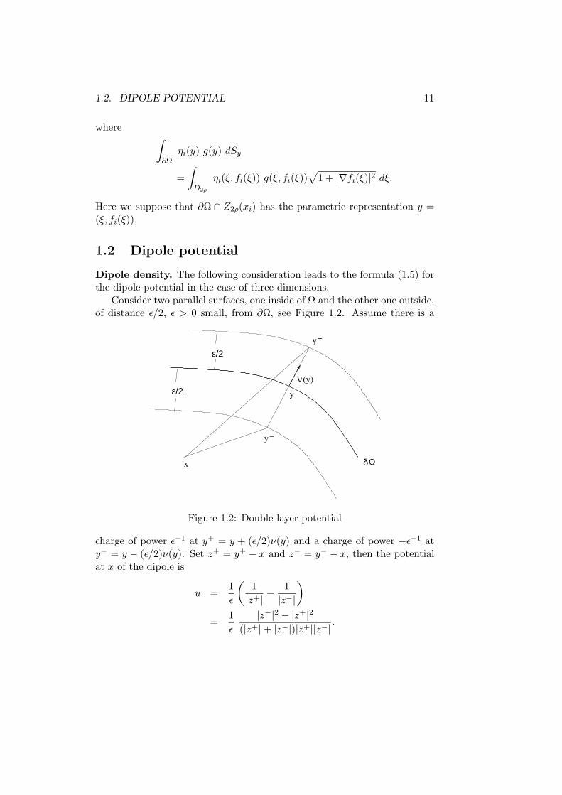
1.2 Dipole potential
Dipole density. The following consideration leads to the formula (1.5) forthe dipole potential in the case of three dimensions.
Consider two parallel surfaces, one inside of Ω and the other one outside,of distance ε/2, ε > 0 small, from ∂Ω, see Figure 1.2. Assume there is a
x
y
y
ε/2
ε/2
δΩ
+
−
y
ν (y)
Figure 1.2: Double layer potential
charge of power ε−1 at y+ = y + (ε/2)ν(y) and a charge of power −ε−1 aty− = y − (ε/2)ν(y). Set z+ = y+ − x and z− = y− − x, then the potentialat x of the dipole is
u =1
ε
(
1
|z+| −1
|z−|
)
=1
ε
|z−|2 − |z+|2(|z+| + |z−|)|z+||z−| .

12 CHAPTER 1. POTENTIAL THEORY
Since z− = z+ − εν(y), we have
|z−|2 = 〈z+ − εν(y), z+ − εν(y)〉= |z+|2 − 2εz+ · ν(y) + ε2.
Thus
u = −1
ε
2εz+ · ν(y) + ε2
(|z+| + |z−|)|z+||z−| .
Set z = y − x, then
limε→0
u = −z · ν(y)
|z|3
=∂
∂ν(y)
(
1
|y − x|
)
is the potential of a single dipole with density σ(y) = 1 at y. Multiplicationwith a density σ(y) and integration over ∂Ω leads to (1.5).
The right hand side of (1.5) is called dipole potential or potential of a doublelayer with density σ. The dipole potential is in C∞(Rn \∂Ω) and a solutionof the Laplace equation in R
n \ ∂Ω. In fact, see the following proposition,the right hand side of (1.5) is defined and continuous on ∂Ω provided theboundary ∂Ω is sufficiently smooth, but W (x) makes a jump across ∂Ω.
Some of the following calculations are based on the formula for the di-rectional derivative in direction ν(y)
∂
∂ν(y)
(
1
|z − y|n−2
)
=1
|z − y|nn
∑
i=1
(zi − yi)(ν(y))i. (1.7)
Lemma 1.2.1. Assume ∂Ω ∈ C1,λ and σ ∈ C(∂Ω). Then the right handside of (1.5) is defined and is continuous on ∂Ω.
Proof. Consider the case n ≥ 3. Let x be the center of a local coordinatesystem and z ∈ ∂Ω ∩ Z2ρ(x), see Figure 1.3. We have to show that, seeSection 1.1 for the definition of the surface integral and formula (1.7),
q(ζ) :=
∫
D2ρ
η(ξ, f(ξ)) σ(ξ, f(ξ))−(ζ − ξ) · ∇f(ξ) + f(ζ) − f(ξ)
(|ζ − ξ|2 + |f(ζ) − f(ξ)|2)n/2dξ
is continuous in a neighbourhood of 0 ∈ Rn−1. Here is D2ρ = D2ρ(0),
z = (ζ, f(ζ)) and y = (ξ, f(ξ)) in local coordinates, and η ∈ C∞ in itsarguments.
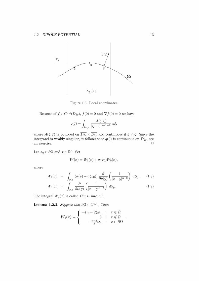
1.2. DIPOLE POTENTIAL 13
T
Z
x
2ρ
δΩ
(x )
xyz
(y)ν
Figure 1.3: Local coordinates
Because of f ∈ C1,λ(D2ρ), f(0) = 0 and ∇f(0) = 0 we have
q(ζ) =
∫
D2ρ
A(ξ, ζ)
|ξ − ζ|n−1−λdξ,
where A(ξ, ζ) is bounded on D2ρ × D2ρ and continuous if ξ 6= ζ. Since theintegrand is weakly singular, it follows that q(ζ) is continuous on D2ρ, seean exercise. 2
Let x0 ∈ ∂Ω and x ∈ Rn. Set
W (x) = W1(x) + σ(x0)W0(x),
where
W1(x) =
∫
∂Ω(σ(y) − σ(x0))
∂
∂ν(y)
(
1
|x − y|n−2
)
dSy, (1.8)
W0(x) =
∫
∂Ω
∂
∂ν(y)
(
1
|x − y|n−2
)
dSy. (1.9)
The integral W0(x) is called Gauss integral.
Lemma 1.2.2. Suppose that ∂Ω ∈ C1,λ. Then
W0(x) =
−(n − 2)ωn : x ∈ Ω0 : x 6∈ Ω
−n−22
ωn : x ∈ ∂Ω.

14 CHAPTER 1. POTENTIAL THEORY
Proof. (i) If x ∈ Rn \ Ω is fixed, then there is a domain Ω0 ⊃⊃ Ω where
|x − y|2−n ∈ C∞(Ω0) and satisfies the Laplace equation. Then
0 =
∫
Ω4y
(
1
|x − y|n−2
)
dy
=
∫
∂Ω
∂
∂ν(y)
(
1
|x − y|n−2
)
dSy.
(ii) Let x ∈ Ω be fixed, then there is a ball Bρ(x) ⊂ Ω. Then
0 =
∫
Ω\Bρ(x)4y
(
1
|x − y|n−2
)
dy
=
∫
∂Ω
∂
∂ν(y)
(
1
|x − y|n−2
)
dSy −∫
∂Bρ(x)
∂
∂ν(y)
(
1
|x − y|n−2
)
dSy,
where in the second integral ν(y) denotes the exterior unit normal at theboundary of Bρ(x). Using polar coordinates with center at x, we find forthe second integral
∫
∂Bρ(x)
∂
∂ν(y)
(
1
|x − y|n−2
)
dSy =
∫
∂B1(x)
∂
∂ρ
(
ρ2−n)
ρn−1 dS
= (2 − n)ωn.
(iii) Let x ∈ ∂Ω and set for a sufficiently small ρ > 0,
Sρ = Ω ∩ ∂Bρ(x), Cρ = ∂Ω \ Bρ(x),
see Figure 1.4. Then
0 =
∫
Ω\Bρ(x)4y
(
1
|x − y|n−2
)
dy
=
∫
Cρ
∂
∂ν(y)
(
1
|x − y|n−2
)
dSy −∫
Sρ
∂
∂ν(y)
(
1
|x − y|n−2
)
dSy.
Since, see an exercise,
limρ→0
∫
Cρ
∂
∂ν(y)
(
1
|x − y|n−2
)
dSy =
∫
∂Ω
∂
∂ν(y)
(
1
|x − y|n−2
)
dSy,
1.2. DIPOLE POTENTIAL 15
B
y
x
y S
Ω
ν
νρ
ρ
(y)
(y)
Cρ
Figure 1.4: Figure to the proof of Lemma 1.2.2
it follows that∫
∂Ω
∂
∂ν(y)
(
1
|x − y|n−2
)
dSy = limρ→0
∫
Sρ
∂
∂ν(y)
(
1
|x − y|n−2
)
dSy.
We have∫
Sρ
∂
∂ν(y)
(
1
|x − y|n−2
)
dSy = −(n − 2)ρ1−n
∫
Sρ
dSy
and∫
Sρ
dSy =ωn
2ρn−1
(
1 + O(ρ2λ))
.
The previous formula follows by introducing local coordinates at x. Let(ξ, h(ξ)) ∈ ∂Bρ(x) ∩ ∂Ω, then
|h(ξ)| ≤ cρ1+λ.
Let F be a layer of a sphere with radius ρ of hight cρ1+λ, see Figure 1.5,then
ωn
2ρn−1 − |F | ≤ |Sρ| ≤
ωn
2ρn−1 + |F |.
We have
|F | =1
2ρn−1ωn(1 − cos θ)
=1
2ρn−1ωn
(
1 − (1 − c2ρ2λ)1/2)
=1
2ρn−1ωnO(ρ2λ)

16 CHAPTER 1. POTENTIAL THEORY
θ
δΩρ
Figure 1.5: Estimate of |Sρ|
as ρ → 0. 2
Lemma 1.2.3. Let ∂Ω ∈ C1,λ. Then∫
∂Ω
∣
∣
∣
∣
∂
∂ν(y)
(
1
|x − y|n−2
)∣
∣
∣
∣
dSy
is uniformly bounded for x ∈ Rn.
Proof. (i) For fixed d > 0 consider x such that dist(x, ∂Ω) ≥ d/2. Then, seeformula (1.7),
∣
∣
∣
∣
∂
∂ν(y)
(
1
|x − y|n−2
)∣
∣
∣
∣
≤ (n − 2)2n−1
dn−1,
which implies that∫
∂Ω
∣
∣
∣
∣
∂
∂ν(y)
(
1
|x − y|n−2
)∣
∣
∣
∣
dSy ≤ (n − 2)2n−1
dn−1|∂Ω|.
(ii) Consider x ∈ Rn such that dist(x, ∂Ω) < d/2 for a d > 0 and let
x0 ∈ ∂Ω : |x − x0| = miny∈∂Ω
|x − y|.
Set Sd = ∂Ω ∩ Bd(x0). Then for y ∈ ∂Ω \ Sd we have
|y − x| ≥ |y − x0| − |x − x0| > d/2,
which implies that∫
∂Ω\Sd
∣
∣
∣
∣
∂
∂ν(y)
(
1
|x − y|n−2
)∣
∣
∣
∣
dSy ≤ (n − 2)2n−1
dn−1|∂Ω \ Sd|
≤ (n − 2)2n−1
dn−1|∂Ω|.
1.2. DIPOLE POTENTIAL 17
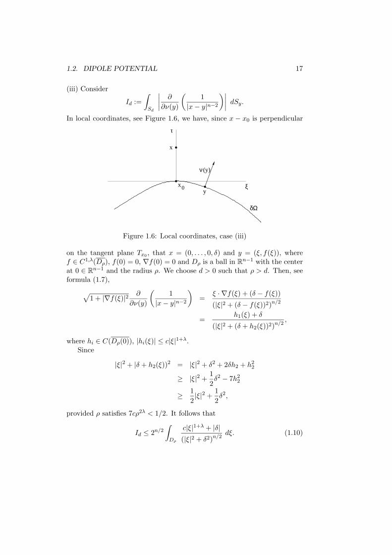
(iii) Consider
Id :=
∫
Sd
∣
∣
∣
∣
∂
∂ν(y)
(
1
|x − y|n−2
)∣
∣
∣
∣
dSy.
In local coordinates, see Figure 1.6, we have, since x − x0 is perpendicular
δΩ
xy
x
0 ξ
τ
(y)ν
Figure 1.6: Local coordinates, case (iii)
on the tangent plane Tx0, that x = (0, . . . , 0, δ) and y = (ξ, f(ξ)), where
f ∈ C1,λ(Dρ), f(0) = 0, ∇f(0) = 0 and Dρ is a ball in Rn−1 with the center
at 0 ∈ Rn−1 and the radius ρ. We choose d > 0 such that ρ > d. Then, see
formula (1.7),
√
1 + |∇f(ξ)|2 ∂
∂ν(y)
(
1
|x − y|n−2
)
=ξ · ∇f(ξ) + (δ − f(ξ))
(|ξ|2 + (δ − f(ξ))2)n/2
=h1(ξ) + δ
(|ξ|2 + (δ + h2(ξ))2)n/2
,
where hi ∈ C(Dρ(0)), |hi(ξ)| ≤ c|ξ|1+λ.Since
|ξ|2 + |δ + h2(ξ))2 = |ξ|2 + δ2 + 2δh2 + h2
2
≥ |ξ|2 +1
2δ2 − 7h2
2
≥ 1
2|ξ|2 +
1
2δ2,
provided ρ satisfies 7cρ2λ < 1/2. It follows that
Id ≤ 2n/2
∫
Dρ
c|ξ|1+λ + |δ|(|ξ|2 + δ2)n/2
dξ. (1.10)

18 CHAPTER 1. POTENTIAL THEORY
The right hand side of (1.10) is uniformly bounded with respect to |δ| < d.More precisely, we have
Id ≤ 2n/2ωn−1 maxcλ−1ρλ, π/2,
see an exercise. 2
Lemma 1.2.4. Assume σ ∈ C(∂Ω) and x0 ∈ ∂Ω. Then W1(x), see defini-tion (1.8), is continuous at x0.
Proof. Set Sρ = ∂Ω ∩ Bρ(x0) and W1(x) = I1 + I2, where
I1(x) =
∫
Sρ
(σ(y) − σ(x0))∂
∂ν(y)
(
1
|x − y|n−2
)
dSy
I2(x) =
∫
∂Ω\Sρ
(σ(y) − σ(x0))∂
∂ν(y)
(
1
|x − y|n−2
)
dSy.
We have
|W1(x) − W1(x0)| ≤ |I1(x)| + |I1(x0)| + |I2(x) − I2(x0)|
and
|I1(x)| ≤∫
Sρ
|σ(y) − σ(x0)|∣
∣
∣
∣
∂
∂ν(y)
(
1
|x − y|n−2
)∣
∣
∣
∣
dSy.
Set, see Lemma 1.2.3,
C = supx∈Rn
∫
∂Ω
∣
∣
∣
∣
∂
∂ν(y)
(
1
|x − y|n−2
)∣
∣
∣
∣
dSy
and choose for given ε > 0 a ρ = ρ(ε) such that
|σ(y) − σ(x0)| <ε
3C
if y ∈ Sρ. Then |I1(x)| < ε/3 and |I1(x0)| < ε/3.
Consider x ∈ Rn such that |x − x0| < ρ/2, then
|y − x| ≥ |y − x0| − |x − x0| ≥ ρ/2,
provided that y ∈ ∂Ω \ Sρ. Since I2 is continuous in Bρ/2(x0), there is aδ = δ(ε) such that
|I2(x) − I2(x0)| < ε/3

1.2. DIPOLE POTENTIAL 19
if |x − x0| < δ(ε). Summarizing, we have
|W1(x) − W1(x0)| < ε
if |x − x0| < minρ(ε)/2, δ(ε). 2
Let x0 ∈ ∂Ω and denote by Wi(x0) the limit of W (x) from interior to x0
and by We(x0) the limit of W (x) from exterior to x0.
Proposition 1.2.1. Suppose that σ ∈ C(∂Ω) and x0 ∈ ∂Ω. The limitsWi(x0) and We(x0) exist and satisfy the jump relations
Wi(x0) = −(n − 2)ωn
2σ(x0) + W (x0),
We(x0) =(n − 2)ωn
2σ(x0) + W (x0).
Proof. We will prove the first of the jump relations. For x ∈ Ω we set W (x) =W1(x) + σ(x0)W0(x), where W1(x) is continuous at x0, see Lemma 1.2.4,and W0(x) is the Gauss integral, see Lemma 1.2.2. Thus
Wi(x0) = limx→x0,x∈Ω
(W1(x) + σ(x0)W0(x))
= W1(x0) − (n − 2)σ(x0)
=
∫
∂Ω(σ(y) − σ(x0))
∂
∂ν(y)
(
1
|x0 − y|n−2
)
dSy − (n − 2)σ(x0)
= W (x0) −(n − 2)ωn
2σ(x0).
2
Corollary. The double layer potential
W (x) =
∫
∂Ωσ(y)
∂
∂ν(y)
(
1
|x − y|n−2
)
dSy,
where σ ∈ C(∂Ω), defines a solution of the interior Dirichlet problem (Di)if and only if σ ∈ C(∂Ω) is a solution of the integral equation
Φ(x) = −(n − 2)ωn
2σ(x) +
∫
∂Ωσ(y)
∂
∂ν(y)
(
1
|x − y|n−2
)
dSy,

20 CHAPTER 1. POTENTIAL THEORY
where x ∈ ∂Ω, and W (x) is a solution of the exterior Dirichlet problem (De)if and only if σ ∈ C(∂Ω) satisfies the integral equation
Φ(x) =(n − 2)ωn
2σ(x) +
∫
∂Ωσ(y)
∂
∂ν(y)
(
1
|x − y|n−2
)
dSy
We recall that W is a solution of (Di) if and only if
Φ(x) = limz→x,z∈Ω
W (z),
and of (De) if and only if
Φ(x) = limz→x,z∈Rn\Ω
W (z).
1.3 Single layer potential
Consider the single layer potential
V (x) =
∫
∂Ω
σ(y)
|x − y|n−2dSy,
where σ ∈ C(∂Ω).
Lemma 1.3.1. V ∈ C(Rn).
Proof. It remains to show that V (x) is continuous if x ∈ ∂Ω. Let x ∈ ∂Ω,set Sρ = ∂Ω ∩ Bρ(x), ρ > 0 sufficiently small, and
V (x) = V1(x) + V2(x),
where
V1(x) =
∫
Sρ
σ(y)
|x − y|n−2dSy,
V2(x) =
∫
∂Ω\Sρ
σ(y)
|x − y|n−2dSy.
Consider z ∈ Rn, z in a neighbourhood of x. We have
|V (z) − V (x)| ≤ |V1(z)| + |V1(x)| + |V2(z) − V2(x)|.

1.3. SINGLE LAYER POTENTIAL 21
δΩ
x
y
ξ
z
ρ
ζ
Figure 1.7: Proof of Lemma 1.3.1
In local coordinates it is y = (ξ, f(ξ)), z = (ζ, δ), where ξ, ζ ∈ Dρ = Dρ(0),see Figure 1.7, and
|V1(z)| ≤∫
Dρ
|σ(ξ, f(ξ))|√
1 + |∇f(ξ)|2(|ζ − ξ|2 + (δ − f(ξ))2)(n−2)/2
dξ
≤ c
∫
Dρ
dξ
|ξ − ζ|n−2
≤ c
∫
D2ρ
dξ
|ξ|n−2
= 2cωn−1ρ.
Let ε > 0 be given and set ρ = ρ(ε) = ε/(6cωn−1), then |V1(z)| < ε/3 if|z − x| < ρ(ε). Consequently, for those z we have
|V (z) − V (x)| ≤ 2
3ε + |V2(z) − V2(x)|.
For fixed ρ > 0 there is a δ = δ(ε) > 0 such that
|V2(z) − V2(x)| <ε
3
if |z − x| < δ(ε). Summarizing, we have
|V (z) − V (x)| < ε,

22 CHAPTER 1. POTENTIAL THEORY
provided that |z − x| < minρ(ε), δ(ε). 2
Definition. Assume u ∈ C1(Ω) and ∂Ω ∈ C1,λ. We say that there exists aregular interior normal derivative of u at ∂Ω if the limit
(
∂u(x)
∂ν(x)
)
i
:= limz→x
∂u(z)
∂ν(x)
exists for each x ∈ ∂Ω. Here is z ∈ Ω on the line defined by the exteriornormal νx at x, see Figure 1.8, and this limit is uniform with respect x ∈ ∂Ωand it is a continuous function on ∂Ω. Analogously, we define the regular
Ω
x
Bρν
z
ξ
(x)
Figure 1.8: Normal derivative
exterior normal derivative of u ∈ C1(Rn \ Ω) on ∂Ω by
(
∂u(x)
∂ν(x)
)
e
:= limz→x
∂u(z)
∂ν(x),
where z ∈ Rn \ Ω is on the line defined by ν(x) and x.
Assume z 6∈ ∂Ω, then
∂V (z)
∂l=
∫
∂Ωσ(y)
∂
∂l
(
1
|z − y|n−2
)
dSy,
where l is any direction. If x ∈ ∂Ω we define
∂V (x)
∂ν(x):=
∫
∂Ωσ(y)
∂
∂ν(x)
(
1
|x − y|n−2
)
dSy. (1.11)

1.3. SINGLE LAYER POTENTIAL 23
In some of the following considerations we need the formula
∂
∂ν(x)
(
1
|x − y|n−2
)
= − n − 2
|x − y|nn
∑
i=1
(xi − yi)(ν(x))i. (1.12)
Lemma 1.3.2. The right hand side of (1.11) exists1 if x ∈ ∂Ω.
Proof. We introduce a local coordinate system with center at x as in previousconsiderations and show that
Iρ(x) :=
∫
Sρ
σ(y)∂
∂ν(x)
(
1
|x − y|n−2
)
dSy
exists, where Sρ = ∂Ω∩Bρ(x), ρ > 0 sufficiently small. In local coordinatesit is y = (ξ, f(ξ)). Using formula (1.12), we obtain
|Iρ(x)| ≤ c1
∫
Dρ
|f(ξ)||ξ|n dξ
≤ c2
∫
Dρ|ξ|−n+1+λ dξ
= c2ωn−1λ−1ρλ.
2
Let x ∈ ∂Ω and consider the sum
s(z) =∂V (z)
∂ν(x)+ W (z)
=
∫
∂Ωσ(y)
(
∂
∂ν(x)
(
1
|z − y|n−2
)
+∂
∂ν(y)
(
1
|z − y|n−2
))
dSy,
where W is the dipole potential and z is on the line defined by ν(x), seeFigure 1.8.
Lemma 1.3.3. The sum s(z) is continuous at x.
Proof. Set Sρ = ∂Ω ∩ Bρ(x), ρ > 0 sufficiently small, and
s(z) = s1(z) + s2(z),
1i. e., this weakly singular exists in the sense of Riemann or as a Lebesgue integral,and it is bounded

24 CHAPTER 1. POTENTIAL THEORY
where
s1(z) =
∫
Sρ
σ(y)
(
∂
∂ν(x)
(
1
|z − y|n−2
)
+∂
∂ν(y)
(
1
|z − y|n−2
))
dSy,
s2(z) =
∫
∂Ω\Sρ
σ(y)
(
∂
∂ν(x)
(
1
|z − y|n−2
)
+∂
∂ν(y)
(
1
|z − y|n−2
))
dSy.
We have
|s(z) − s(x)| ≤ |s1(z)| + |s1(x)| + |s2(z) − s2(x)|.
Thus the lemma is shown if for given ε > 0 there exists a ρ = ρ(ε) > 0 suchthat |s1(z)| < ε/3 if |x − z| < ρ(ε), see the proof of Lemma 1.3.1. It is,see (1.7), (1.12),
∂
∂ν(x)
(
1
|z − y|n−2
)
+∂
∂ν(y)
(
1
|z − y|n−2
)
= (n − 2)1
|z − y|n
(
n∑
i=1
(zi − yi)(ν(y))i −n
∑
i=1
(zi − yi)(ν(x))i
)
,
where, in local coordinates, x = (0, . . . , 0, 0), z = (0, . . . , 0, δ), ν(x) =(0, . . . , 0, 1) and
ν(y) =1
√
1 + |∇f(ξ)|2(−fξ1 , . . . ,−fξn−1
, 1).
It follows that
|s1(z)| ≤ c1
∫
Sρ
∣
∣
∣
∣
∂
∂ν(x)
(
1
|z − y|n−2
)
+∂
∂ν(y)
(
1
|z − y|n−2
)∣
∣
∣
∣
dSy
≤ c2
∫
Dρ(0)
∣
∣
∣ξ · ∇f(ξ) + (δ − f(ξ)) − δ
√
1 + |∇f(ξ)|2∣
∣
∣
(|ξ|2 + |δ − f(ξ)|2)n/2dξ
≤ c3
∫
Dρ(0)
|ξ|1+λ + |δ||ξ|2λ
(|ξ|2 + δ2)n/2dξ
≤ c3ωn−1 maxλ−1ρλ, πρ2λ/2,
where the constants ci are independent of ρ. 2
Proposition 1.3.1. Suppose that ∂Ω ∈ C1,λ. Then there exists a regularinterior and a regular exterior normal derivative of V , and these derivatives
1.3. SINGLE LAYER POTENTIAL 25
satisfy the jump relations(
∂V (x)
∂ν(x)
)
i
=(n − 2)ωn
2σ(x) +
∂V (x)
∂ν(x)(
∂V (x)
∂ν(x)
)
e
= −(n − 2)ωn
2σ(x) +
∂V (x)
∂ν(x),
where x ∈ ∂Ω.
Proof. The existence of regular normal derivatives follow from Lemma 1.3.3and Proposition 1.2.1 since
∂V (z)
∂ν(x)=
(
∂V (z)
∂νx+ W (z)
)
− W (z),
where z is on the line defined by ν(x). From Lemma 1.3.3 it follows also
(
∂V (x)
∂ν(x)
)
i
+ Wi(x) =
(
∂V (x)
∂ν(x)
)
e
+ We(x)
=∂V (x)
∂ν(x)+ W (x),
where
∂V (x)
∂ν(x): =
∫
∂Ωσ(y)
∂
∂ν(x)
(
1
|x − y|n−2
)
dSy,
W (x) : =
∫
∂Ωσ(y)
∂
∂ν(y)
(
1
|x − y|n−2
)
dSy.
Using Lemma 1.3.1, we obtain(
∂V (x)
∂ν(x)
)
i
= W (x) − Wi(x) +∂V (x)
∂ν(x)
=(n − 2)ωn
2σ(x) +
∂V (x)
∂ν(x)
and(
∂V (x)
∂ν(x)
)
e
= W (x) − We(x) +∂V (x)
∂νx
= −(n − 2)ωn
2σ(x) +
∂V (x)
∂ν(x).
2

26 CHAPTER 1. POTENTIAL THEORY
Remark. Let x ∈ ∂Ω, then it follows immediately that(
∂V (x)
∂ν(x)
)
i
−(
∂V (x)
∂νx
)
e
= (n − 2)ωnσ(x).
Corollary. The single layer potential
V (x) =
∫
∂Ω
σ(y)
|x − y|n−2dSy,
where σ ∈ C(∂Ω) defines a solution of the interior Neumann problem (Ni)if and only if σ ∈ C(∂Ω) is a solution of the integral equation
Ψ(x) =(n − 2)ωn
2σ(x) +
∫
∂Ωσ(y)
∂
∂ν(x)
(
1
|x − y|n−2
)
dSy,
where x ∈ ∂Ω, and V (x) is a solution of the exterior Neumann problem (Ne)if and only if σ ∈ C(∂Ω) satisfies the integral equation
Ψ(x) = −(n − 2)ωn
2σ(x) +
∫
∂Ωσ(y)
∂
∂ν(x)
(
1
|x − y|n−2
)
dSy.
We recall that V is a solution of (Ni) if and only if
Ψ(x) =
(
∂V (x)
∂ν(x)
)
i
,
and of (Ne) if and only if
Ψ(x) =
(
∂V (x)
∂ν(x)
)
e
.
1.4 Integral equations
Denote by H = L2(∂Ω) the Hilbert space with the inner product
〈σ, µ〉 =
∫
∂Ωσ(x)µ(x) dSx,
and, if n ≥ 3, we define the linear operator T from H into H by
(Tσ)(x) =
∫
∂Ωσ(y)
∂
∂ν(y)
(
1
|x − y|n−2
)
dSy.
1.4. INTEGRAL EQUATIONS 27
Set
(T ∗σ)(x) =
∫
∂Ωσ(y)
∂
∂ν(x)
(
1
|x − y|n−2
)
dSy,
then
〈Tσ, µ〉 = 〈σ, T ∗µ〉
for all σ, µ ∈ H. Below we will show that T is bounded. Then it followsthat T ∗ is the adjoint operator to T .
According to the above corollaries to Proposition 1.2.1 and Proposi-tion 1.3.1, the potentials W and V are solutions of the boundary valueproblems (Di), De), (Ni) and (Ne) if the density σ is continuous on ∂Ω andsatisfies the integral equations, respectively,
σ − 2
(n − 2)ωnTσ = − 2
(n − 2)ωnΦ (Di)I
σ +2
(n − 2)ωnTσ =
2
(n − 2)ωnΦ (De)I
σ +2
(n − 2)ωnT ∗σ =
2
(n − 2)ωnΨ (Ni)I
σ − 2
(n − 2)ωnT ∗σ = − 2
(n − 2)ωnΨ (Ne)I .
Remark. Since we make the ansatz with above potentials for the exteriorproblems, we prescribe in fact the behaviour |u(z) ≤ c|z|1−n, |u(z) ≤ c|z|2−n,respectively, as z → ∞.
The above integral equations are defined for σ ∈ L2(∂Ω). In the following wewill discuss whether or not there exist solutions in L2(∂Ω). From a regularityresult which says that an L2-solution is in fact in C(∂Ω), we recover that thepotentials define solutions of the boundary value problem, see the corollariesto Proposition 1.2.1 and Proposition 1.3.1.
Proposition 1.4.1. Suppose that ∂Ω ∈ C1,λ. Then T is a completelycontinuous operator from H into H.
Proof. (i) T is bounded. It is sufficient, see Section 1.1, to show that
(Pµ)(ζ) :=
∫
Dρ
a(ξ)µ(ξ)K(ξ, ζ) dξ

28 CHAPTER 1. POTENTIAL THEORY
is bounded from L2(Dρ) into L2(Dρ). Here is Dρ = Dρ(0) ⊂ Rn−1, a ∈
C∞0 (Dρ), µ(ξ) = σ(ξ, f(ξ)) and
K(ξ, ζ) =(n − 2) (−(ξ − ζ) · ∇f(ξ) + f(ζ) − f(ξ))
(|ξ − ζ|2 + (f(ξ) − f(ζ))2)n/2.
Set q(ζ) := (Pµ)(ζ), then
q(ζ) =
∫
Dρ
µ(ξ)A(ξ, ζ)
|ξ − ζ|n−1−λdξ,
where A is bounded on Dρ×Dρ) and continuous if ξ 6= ζ. Let κ = n−1−λ,then we have, with constants ci independent of µ and ρ, that
|q(ζ)| ≤ c1
∫
Dρ
|µ(ξ)||ξ − ζ|κ/2
1
|ξ − ζ|κ/2dξ,
|q(ζ)|2 ≤ c2
∫
Dρ
|µ(ξ)|2|ξ − ζ|κ dξ
∫
Dρ
dξ
|ξ − ζ|κ
≤ c3ρλ
∫
Dρ
|µ(ξ)|2|ξ − ζ|κ dξ,
∫
Dρ
|q(ζ)|2 dζ ≤ c3ρλ
∫
Dρ
|µ(ξ)|2(
∫
Dρ
dζ
|ξ − ζ|κ
)
dξ
≤ c4ρ2λ
∫
Dρ
|µ(ξ)|2 dξ.
(ii) T is completely continuous. According to a lemma due to Kolmogoroff,see for example [21], pp. 246, or [1], pp. 31, P is completely continuous iffor given ε1 > 0 there exists an h0(ε1) > 0 such that
∫
Dρ
|q(ζ + h) − q(ζ)|2 dζ ≤ ε21
for all h ∈ Rn−1 such that |h| ≤ h0(ε1), and uniformly for ||µ||L2(Dρ) ≤ M ,
where M < ∞. Thus the set ||µ||L2(Dρ) ≤ M is uniformly continuous in themean. Above we set q(ζ) = 0 if ζ 6∈ Dρ. Let η ∈ C(R+), 0 ≤ η ≤ 1, suchthat for given ε > 0
η(t) =
1 : 0 ≤ t ≤ ε/20 : t ≥ ε
.
1.4. INTEGRAL EQUATIONS 29
Set
q(ζ) = q1(ζ) + q2(ζ),
where
q1(ζ) =
∫
Dρ(0)µ(ξ)
A(ξ, ζ)η(|ξ − ζ|)|ξ − ζ|κ dξ
q2(ζ) =
∫
Dρ(0)µ(ξ)
A(ξ, ζ) (1 − η(|ξ − ζ|))|ξ − ζ|κ dξ.
We have
|q(ζ + h) − q(ζ)| ≤ |q1(ζ + h)| + |q1(ζ)| + |q2(ζ + h) − q2(ζ)|. (1.13)
Let ε > 0 be fixed, then for given τ > 0 there is an h0 = h0(τ) > 0 such that
|q2(ζ) − q2(ζ)| < τ (1.14)
for all |h| ≤ h0. Concerning q1(ζ) we have
|q1(ζ)| ≤ c
∫
Dρ(0)∩Bε(ζ)|µ(ξ)| dξ
|ξ − ζ|κ
|q1(ζ)|2 ≤ c2
∫
Dρ(0)∩Bε(ζ)|µ(ξ)|2 dξ
|ξ − ζ|κ∫
Dρ(0)∩Bε(ζ)
dξ
|ξ − ζ|κ
≤ c2ωn−1ελλ−1
∫
Dρ(0)∩Bε(ζ)|µ(ξ)|2 dξ
|ξ − ζ|κ∫
Dρ(0)|q1(ζ)|2 dζ ≤ c2ωn−1ε
λλ−1
∫
Dρ(0)
∫
Dρ(0)|µ(ξ)|2 dξ
|ξ − ζ|κ dζ
= c2ωn−1ελλ−1
∫
Dρ(0)|µ(ξ)|2 dξ
∫
Dρ(0)
dζ
|ξ − ζ|κ
≤ c2ωn−1ελλ−1
∫
Dρ(0)|µ(ξ)|2 dξ
∫
D2ρ(ξ)
dζ
|ξ − ζ|κ
= c2ω2n−1ε
λλ−2(2ρ)λ||µ||2L2(Dρ).

30 CHAPTER 1. POTENTIAL THEORY
Analogously we have
|q1(ζ + h)|2 ≤ c2
∫
Dρ(0)∩Bε(ζ+h)|µ(ξ)|2 dξ
|ξ − (ζ + h)|κ∫
Dρ(0)∩Bε(ζ+h)
dξ
|ξ − (ζ + h)|κ
≤ c2ωn−1ελλ−1
∫
Dρ(0)∩Bε(ζ+h)|µ(ξ)|2 dξ
|ξ − (ζ + h)|κ∫
Dρ(0)|q1(ζ + h)|2 dζ ≤ c2ωn−1ε
λλ−1
∫
Dρ(0)
∫
Dρ(0)|µ(ξ)|2 dξ
|ξ − (ζ + h)|κ dζ
= c2ωn−1ελλ−1
∫
Dρ(0)|µ(ξ)|2 dξ
∫
Dρ(0)
dζ
|ξ − (ζ + h)|κ
≤ c2ωn−1ελλ−1
∫
Dρ(0)|µ(ξ)|2 dξ
∫
D3ρ(ξ−h)
dζ
|ζ − (ξ − h)|κ
= c2ω2n−1ε
λλ−2(3ρ)λ||µ||2L2(Dρ).
Combining these L2-estimates with (1.13) and (1.14) we obtain that themapping T is completely continuous. 2
From a result of functional analysis we have
Corollary. T ∗ is bounded with the same norm as T and T ∗ is completelycontinuous.
In the following we study the question of the existence of solutions σ ∈L2(∂Ω) of the above integral equations. To recover that the associatedsurface potentials define solutions of the original boundary value problems,we need more regularity, namely σ ∈ C(∂Ω). We obtain this property byusing the integral equations.
Proposition 1.4.2 (Regularity). Let w ∈ L2(Dρ) be a solution of theintegral equation
w(ζ) −∫
Dρ
w(ξ)A(ξ, ζ)
|ξ − ζ|κ dξ = b(ζ),
where κ = n − 1 − λ, Dρ = Dρ(0) ⊂ Rn−1, A is bounded in Dρ × Dρ and

1.4. INTEGRAL EQUATIONS 31
continuous if ξ 6= ζ. The function b ∈ C(Dρ) is given. Then it follows thatw ∈ C(Dρ).
Proof. Let η ∈ C(R+), 0 ≤ η ≤ 1, such that for given ε > 0
η(t) =
1 : 0 ≤ t ≤ ε/20 : t ≥ ε
.
SetA(ξ, ζ)
|ξ − ζ|κ = K1(ξ, ζ) + K2(ξ, ζ),
where
K1(ξ, ζ) =A(ξ, ζ)η(|ξ − ζ|)
|ξ − ζ|κ
K2(ξ, ζ) =A(ξ, ζ) (1 − η(|ξ − ζ|)
|ξ − ζ|κ .
Then
w(ζ) −∫
Dρ
w(ξ)K1(ξ, ζ) dξ = g(ζ),
where
g(ζ) =
∫
Dρ
w(ξ)K2(ξ, ζ) dξ + b(ζ)
is a continuous function on Dρ. Define the integral operator T1 from L2(Dρ)into L2(Dρ) by
(T1w)(ζ) =
∫
Dρ
w(ξ)K1(ξ, ζ) dξ,
then we can write the above integral equation as (I − T1)w = g, where Idenotes the identity operator. The L2-norm of T1 satisfies the inequality||T1|| < 1, provided ε > 0 is sufficiently small, see an exercise. It followsthat w is given by the Neumann series
w = (I − T1)−1g =
∞∑
n=0
Tn1 g,
which is a uniformly convergent series of continuous functions, providedε > 0 was chosen sufficiently small, see an exercise. 2
FREDHOLM THEOREMS. Here we recall some results from functionalanalysis, see for example [23]. Let H be a Hilbert space over C and T : H 7→

32 CHAPTER 1. POTENTIAL THEORY
H a completely continuous linear operator. Consider for given f, g ∈ Hand λ ∈ C the equations
u + λ Tu = f (I)
v + λ T ∗v = g (I∗)
and the associated homogeneous equations
u + λ Tu = 0 (Ih)
v + λ T ∗v = 0 (I∗h).
Equations (I∗), (I∗h) are called adjoint to (I), (Ih), respectively.
(i) Let λ be an eigenvalue of (Ih), then the linear space of solutions hasfinite dimension.
(ii) The eigenvalue problem (Ih) has at most a countable set of eigenvalueswith at most one limit element at infinity.
(iii) λ is an eigenvalue of (Ih) if and only if λ is an eigenvalue of (I∗h) anddim N(I + λT ) =dim N(I + λT ∗).
(iv) (I) has a solution if and only if f ⊥ N(I+λ T ∗) and (I∗) has a solutionif and only if g ⊥ N(I + λ T ).
We recall that N(A) denotes the null space N(A) = w ∈ H : Aw = 0 ofa linear operator A.
Proposition 1.4.3. Suppose that ∂Ω ∈ C2, then λ0 = −2/((n − 2)ωn) isno eigenvalue of the homogeneous integral equation to (Di).
Proof. Suppose that λ0 is an eigenvalue and µ0 ∈ L2(∂Ω) an associatedeigenvector of the adjoint problem (Ne)I . From Proposition 1.4.2 we havethat µ0 ∈ C(∂Ω). Consider the single layer potential
V (x) :=
∫
∂Ω
µ0(y)
|x − y|n−2dSy.
From a jump relation of Proposition 1.3.1 it follows that
(
∂V (x)
∂ν(x)
)
e
= 0 (1.15)

1.4. INTEGRAL EQUATIONS 33
since µ0 is an eigenvector of (Ne)I .Set for a (small) h > 0
Ωh = Ω ∪ y ∈ Rn : y = x + sν(x), x ∈ ∂Ω, 0 ≤ s < h,
see Figure 1.9. The surface ∂Ωh is called parallel surface to ∂Ω.
x
z
h
Ω
δΩ
(x)=ν ν (z)
h
Figure 1.9: Parallel surface
Consider a ball BR = BR(0) such that Ωh ⊂ BR, then
∫
BR\Ωh
|∇V |2 dx =
∫
∂BR
V (x)∂V (x)
∂ν(x)dSx −
∫
∂Ωh
V (z)∂V (z)
∂ν(z)dSz. (1.16)
We have on ∂Ωh
ν(z) = ν(x). (1.17)
To show this equation, we consider the surface ∂Ω which is given (locally)by x = x(u), where u ∈ U and U is an (n-1)-dimensional parameter domain.Then the parallel surface ∂Ωh is defined by z(u) = x(u) + hν(x(u)). Thenwe consider a C1-curve X(t) on ∂Ω with X(0) = x, and let Z(t) be theassociated curve on ∂Ωh. Then
|X(t) − Z(t)|2 = h2.
It follows
(X(t) − Z(t)) · X ′(t) − (X(t) − Z(t)) · Z ′(t) = 0,
which proves (1.17) since the first term is zero.
34 CHAPTER 1. POTENTIAL THEORY
Combining (1.16), (1.17), (1.15) and
limh→0
∂V (z)
∂ν(x)=
(
∂V (x)
∂ν(x)
)
e
,
we obtain
limh→0
∫
BR\Ωh
|∇V |2 dx =
∫
∂BR
V (x)∂V (x)
∂ν(x)dSx
since the surface element dSz converges uniformly to dSx on U as h → 0.2
We have V = O(R2−n) and ∂V/∂ν(x) = O(R1−n), consequently
limR→∞
(
limh→0
∫
BR\Ωh
|∇V |2 dx
)
= 0.
Thus V = const. on Rn \ Ω. From the behaviour of V at infinity it follows
that V ≡ 0 on Rn \ Ω. Because of V ∈ C(Rn), see Lemma 1.3.1.
From the maximum principle we find that V ≡ 0 in Ω since 4V = 0 inΩ and V = 0 on ∂Ω. Consequently the interior regular normal derivativeon ∂Ω is zero. Finally the jump relations, see Proposition 1.3.1, imply thatµ0(x) ≡ 0 on ∂Ω. 2
Proposition 1.4.3 and Fredholm’s theorems imply
Theorem 1.4.1. Let Ω be bounded and ∂Ω ∈ C2. Then there exists forgiven Φ, Ψ ∈ C(∂Ω) a unique solution of the interior Dirichlet problem (Di)and the exterior Neumann problem (Ne), respectively.3
Proof. N(I + λ0T ) = N(I + λ0T∗) = 0. 2
Proposition 1.4.4. Let Ω be bounded and ∂Ω ∈ C2. The number λ0 =2/((n − 2)ωn) is a simple eigenvalue of (De)I to the eigenvector σ ≡ 1.
Proof. From, see Lemma 1.2.2,∫
∂Ω
∂
∂ν(y)
(
1
|x − y|n−2
)
dSy = −(n − 2)ωn
2
2In the case R3 we have dSz =
√EG − F 2du1du2, where E = zu1
· zu1, G = zu2
· zu2,
F = zu1· zu2
and z(u) = x(u) + hν(x(u)).3In this and in the following two theorems it is sufficient to assume that ∂Ω ∈ C
1,1 byRademacher’s Theorem: A Lipschitz continuous function is differentiable almost every-where, see for example [5], pp. 280 or [6].

1.4. INTEGRAL EQUATIONS 35
we see that λ0 is an eigenvalue and σ ≡ 1 is an associated eigenvector. FromFredholm’s theorems it follows that there exists at least one eigenfunctionµ0(x) to λ0 of (Ni)h. We will show that dim N(I + λ0 T ∗) = 1. Set
V (x) =
∫
∂Ω
µ0(y)
|x − y|n−2dSy.
From the jump relations, see Proposition 1.3.1 and from the fact that µ0
is an eigenvector it follows that (∂V (x)/∂ν(x))i = 0. We obtain as in theproof of Proposition 1.4.3 that V (x) = const. =: c0 in Ω. This constant isdifferent from zero. If not, then V = 0 on ∂Ω. Then the maximum principleimplies that V ≡ 0 in R
n \ Ω. We recall that V = O(|x|2−n) as |x| → ∞.Consequently we have also (∂V (x)/∂ν(x))e = 0, which implies that µ0 = 0,see the jump relations of Proposition 1.3.1.
Let µ1 be another eigenvector to λ0, then we can assume that µ1 ∈ C(∂Ω)according to the regularity result Proposition 1.4.2. Set
V1(x) =
∫
∂Ω
µ1(y)
|x − y|n−2dSy.
As above we conclude that V1(x) ≡ const. =: c1 in Ω, where c1 6= 0. Thelinear combination µ2 := c1µ0 − c0µ1 is contained in the null space N(I +λ0 T ∗). Set
V2(x) =
∫
∂Ω
µ2(y)
|x − y|n−2dSy
= c1V0(x) − c0V1(x).
In Ω we have V2(x) = c1c0 − c0c1, and from the jump relations we find asabove that µ2(x) ≡ 0. Thus we have shown
µ1(x) =c1
c0µ0(x).
2
Then it follows from Fredholm’s theorems
Theorem 1.4.2. Let Ω be bounded and ∂Ω ∈ C2. Then there exists asolution of (Ni) if and only if
∫
∂ΩΨ(y) dSy = 0.

36 CHAPTER 1. POTENTIAL THEORY
In fact, we obtain also the existence of a solution of (De)I under the as-sumption that
∫
∂Ωµ0(y)Φ(y) dSy = 0,
where µ0 is the eigenvector from above. It turns out that there is a solution ofthe exterior Dirichlet problem without this restriction if we look for solutionswith a weaker decay at infinity. We make the ansatz of a sum of a doublelayer and a single layer potential
u(x) =
∫
∂Ωσ(y)
∂
∂ν(y)
(
1
|x − y|n−2
)
dSy
+d
∫
∂Ω
µ0(y)
|x − y|n−2dSy,
where d is a constant which we will determine later. The ansatz defines asolution of the exterior Dirichlet problem if and only if
limy→x, y∈Rn\Ω
u(y) = φ(x),
where x ∈ ∂Ω. From a jump relation of Proposition 1.2.1 we see that theunknown density σ must satisfy the integral equation
Φ(x) =
∫
∂Ωσ(y)
∂
∂ν(y)
(
1
|x − y|n−2
)
dSy
+(n − 2)ωn
2σ(x) + d
∫
∂Ω
µ0(y)
|x − y|n−2dSy.
Above we have shown that, if x ∈ ∂Ω,
∫
∂Ω
µ0(y)
|x − y|n−2dSy = const. = c0
with a constant c0 6= 0. Thus we have to consider the integral equation
(n − 2)ωn
2σ(x) +
∫
∂Ωσ(y)
∂
∂ν(y)
(
1
|x − y|n−2
)
dSy = Φ(x) − dc0.
This equation has a solution if∫
∂Ω(Φ(x) − dc0)µ0(x) dSx = 0
1.4. INTEGRAL EQUATIONS 37
is satisfied. We can find an appropriate constant d such that this equationis satisfied since
∫
∂Ωµ0(x) dSx 6= 0.
This inequality is a consequence of a jump relation and of the fact that µ0
is an eigenvector:(
∂V0(x)
∂ν(x)
)
e
= −(n − 2)ωn
2µ0(x) +
∫
∂Ωµ0(y)
∂
∂ν(x)
(
1
|x − y|n−2
)
dSy
0 =(n − 2)ωn
2µ0(x) +
∫
∂Ωµ0(y)
∂
∂ν(x)
(
1
|x − y|n−2
)
dSy,
which implies that(
∂V0(x)
∂ν(x)
)
e
= −(n − 2)ωnµ0(x).
Suppose that∫
∂Ωµ0(x) dSx = 0,
then∫
∂Ω
(
∂V0(x)
∂ν(x)
)
e
dSx = 0,
which implies, see the proof of Proposition 1.4.3 for notations,∫
BR\Ωh
|∇V0|2 dx =
∫
∂BR
V0(x)∂V0(x)
∂ν(x)dSx −
∫
∂Ωh
V0(z)∂V0(z)
∂ν(z)dSz.
Letting h → 0 and R → ∞, it follows V0 = const. in Rn \ Ω and V0 = c0
since V0(x) = const. = c0 on ∂Ω.From the decay behaviour of V0 at infinity and since V ∈ C(Rn) we
find that V0 = 0 in Rn \ Ω. Thus we have c0 = 0, a contradiction to a
consideration above.
Thus we have shown
Theorem 1.4.3. Let Ω be bounded and ∂Ω ∈ C2. Then for given Φ ∈C(∂Ω) there exists a unique solution u of (De) which the property u =O(|x|2−n) as |x| → ∞.
Proof. It remains to show that the solution is unique. This follows from themaximum principle. 2

38 CHAPTER 1. POTENTIAL THEORY
Remark. There is no uniqueness without the decay assumption. Let Ω =BR(0) be a ball in R
3. Then u = 1/|x| and u = 1/R are two solutions of theLaplace equation with the same boundary values on ∂Ω.
1.5 Volume potential
Set
Γ(x, y) = s(|x − y|),
where s(r) is the singularity function
s(r) :=
− 12π
ln r : n = 2r2−n
(n−2)ωn: n ≥ 3
We recall that ωn = |∂B1(0)|. Let Ω ∈ Rn a bounded and sufficiently
regular domain, then we define for given f the volume potential (or Newtonpotential)
V (x) =
∫
ΩΓ(x, y)f(y) dy.
If f is bounded in Ω and f ∈ C1(Ω), then V ∈ C2(Ω) and −4V = f inΩ, see for example [17]. This result holds under the weaker assumptionthat f is bounded and locally Holder continuous in Ω, see Proposition 1.5.1.In fact, also the second derivatives are Holder continuous (with the sameHolder exponent), see [10], for example.
Definition. Let f be a real function, defined in a fixed bounded neighbour-hood D of x0 ∈ R
n. Then f is called Holder continuous at x0 if there existsa real number α, 0 < α ≤ 1, such that
[f ]α,x0:= sup
x∈D\x0
|f(x) − f(x0)||x − x0|α
< ∞.
The constant [f ]α,x0is called Holder constant and α Holder exponent.
The function f is said to be uniformly Holder continuous with respectto α in D if
[f ]α,D := supx,y∈D, x 6=y
|f(x) − f(y)||x − y|α < ∞,
and f is called locally Holder continuous in a domain Ω if f is uniformlyHolder continuous on compact subsets of Ω.

1.5. VOLUME POTENTIAL 39
In the following we will use the abbreviations Di = ∂/∂xi and Dij =∂2/∂xi∂xj .
Proposition 1.5.1. (i) Let f be bounded and integrable over Ω. ThenV ∈ C1(Rn) and for any x ∈ Ω
DiV (x) =
∫
ΩDiΓ(x, y)f(y) dy.
(ii) Let f be bounded and locally Holder continuous in Ω with exponent 0 <α ≤ 1. Then V ∈ C2(Ω), −4V = f in Ω, and for any x ∈ Ω
DijV (x) =
∫
Ω0
DijΓ(x, y)(f(y) − f(x)) dy (1.18)
−f(x)
∫
∂Ω0
DiΓ(x, y)(ν(y))j dSy,
where Ω0 ⊃ Ω is any domain for which the divergence theorem holds and fis extended to vanish outside Ω.
Proof. See [10], Chapter 4. (i) Set for x ∈ Rn
v(x) =
∫
ΩDiΓ(x, y)f(y) dy.
This function is well defined since |DiΓ| ≤ |x − y|1−n/ωn holds. We willshow that v = DiV and v ∈ C(Rn). Let η ∈ C1(R) be a fixed functionsatisfying 0 ≤ η ≤ 1, 0 ≤ η′ ≤ 2, η(t) = 0 if t ≤ 1 and η(t) = 1 if t ≥ 2. Fora (small) ε > 0 set ηε = η(|x − y|/ε) and consider the regularized potential
Vε(x) =
∫
ΩΓ(x, y)ηεf(y) dy.
Then Vε ∈ C1(Rn) and
v(x) − DiVε(x) =
∫
B2ε(x)Di ((1 − ηε)Γ) f(y) dy.
We obtain
|v(x) − DiVε(x)| ≤ supΩ
|f |∫
B2ε(x)(|DiΓ| + 2|Γ|/ε) dy
≤ supΩ
|f |
4(1 + | ln(2ε)|)ε : n = 22nε/(n − 2) : n ≥ 3
.
40 CHAPTER 1. POTENTIAL THEORY
It follows that Vε and DiVε converge uniformly on compact subsets of Rn to
V and v, resp., as ε → 0. Consequently V ∈ C1(Rn) and DiV = v.
(ii) Set for x ∈ Ω
u(x) =
∫
Ω0
DijΓ(x, y)(f(y) − f(x)) dy
−f(x)
∫
∂Ω0
DiΓ(x, y)(ν(y))j dSy.
The right hand side is well-defined since f is locally Holder continuous andsince |DijΓ| ≤ (1 + n)|x − y|n/ωn holds. Set v = DiV and define for ε > 0the regularized function
vε(x) =
∫
Ω0
DiΓηεf(y) dy.
Then
Djvε =
∫
Ω0
Dj(DiΓηε)f(y) dy
=
∫
Ω0
Dj(DiΓηε)(f(y) − f(x)) dy
f(x)
∫
Ω0
Dj(DiΓηε) dy
=
∫
Ω0
Dj(DiΓηε)(f(y) − f(x)) dy
−f(x)
∫
∂Ω0
DiΓ(ν(y))j dSy,
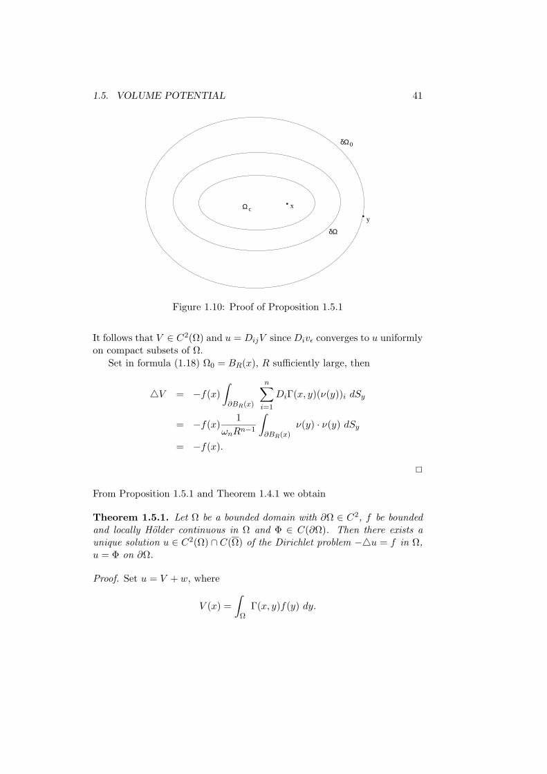
provided ε > 0 is small enough such that ηε = 1 on ∂Ω0, see Figure 1.10.Then
u(x) − Djvε(x) =
∫
B2ε(x)Dj ((1 − ηε)DiΓ) (f(y) − f(x)) dy.
We suppose that 2ε < dist (x, ∂Ω) if x ∈ Ωc, Ωc ⊂⊂ Ω. Then
|u(x) − Djvε(x)| ≤ [f ]α,Ωc
∫
B2ε(x)(|DijΓ| + 2|DiΓ|/ε) |x − y|α dy
≤ [f ]α,Ωc(4 + n/α)(2ε)α.
1.5. VOLUME POTENTIAL 41
Ω
δΩ
y
xc
0
δΩ
Figure 1.10: Proof of Proposition 1.5.1
It follows that V ∈ C2(Ω) and u = DijV since Divε converges to u uniformlyon compact subsets of Ω.
Set in formula (1.18) Ω0 = BR(x), R sufficiently large, then
4V = −f(x)
∫
∂BR(x)
n∑
i=1
DiΓ(x, y)(ν(y))i dSy
= −f(x)1
ωnRn−1
∫
∂BR(x)ν(y) · ν(y) dSy
= −f(x).
2
From Proposition 1.5.1 and Theorem 1.4.1 we obtain
Theorem 1.5.1. Let Ω be a bounded domain with ∂Ω ∈ C2, f be boundedand locally Holder continuous in Ω and Φ ∈ C(∂Ω). Then there exists aunique solution u ∈ C2(Ω) ∩ C(Ω) of the Dirichlet problem −4u = f in Ω,u = Φ on ∂Ω.
Proof. Set u = V + w, where
V (x) =
∫
ΩΓ(x, y)f(y) dy.

42 CHAPTER 1. POTENTIAL THEORY
Then u is a solution of the Dirichlet problem if and only if 4w = 0 in Ω andw = Φ − V on ∂Ω. The existence of a w follows from Theorem 1.4.1. Theuniqueness of u is a consequence of the maximum principle. Moreover, w isgiven by a dipole potential, see Theorem 1.4.1. 2

1.6. EXERCISES 43
1.6 Exercises
1. Let S be a surface in R3 defined by z = f(x), x = (x1, x2), x ∈ U ,
where U is a neighbourhood of x = 0. Assume f ∈ C1,λ(U), f(0) =0, ∇f(0) = 0. Consider the intersection I = S ∩ ∂Bρ0
(0), ρ0 > 0sufficiently small, i. e.,
I = (x, z) : z = f(x) and x21 + x2
2 + z2 = ρ20.
Show that there is a function ε(ρ, φ), 0 < ρ ≤ ρ0, φ ∈ [0, 2π), 2π-periodic in φ and in C1 with respect to φ, such that ε(ρ, φ) = O(ρλ)as ρ → 0, uniformly in φ ∈ [0, 2π), and
x1 = ρ(1 + ε(ρ, φ)) cos φ
x2 = ρ(1 + ε(ρ, φ)) sin φ.
Hint: Implicit function theorem.
2. Let B2R(x0) ⊂ Rn be a ball with radius 2R and the center at x0. Show
that there is a function η ∈ C∞0 (B2R(x0)) which satisfies 0 ≤ η ≤ 1 in
B2R(x0) and η ≡ 1 in BR(x0).
Hint: Set r = |x| and define
φ(r) = e−1/((3/(2R)−r)2−r2/4)
if R < r < 2R and set φ(r) = 0 if 0 < r < R or r ≥ 2R. Let
ψ(r) =
∫ r0 φ(t) dt
∫ ∞0 φ(t) dt
and χ(r) = 1−ψ(r). Show that η(x) = χ(|x−x0|) is a function whichsatisfies the above properties.
3. Suppose that ∂Ω ∈ C1,λ and x ∈ ∂Ω. Show that
limρ→0
∫
∂Ω\Bρ(x)
∂
∂ν(y)
(
1
|z − y|n−2
)
dSy = 0
Hint: Local coordinates and formula (1.7).

44 CHAPTER 1. POTENTIAL THEORY
4. Let Ω ⊂ Rn be a bounded and sufficiently regular domain and set
q(ζ) =
∫
Ω
A(ξ, ζ)
|ξ − ζ|n−λdξ,
where A is bounded in Ω × Ω and continuous if ξ 6= ζ and 0 < λ ≤ 1.Show that q ∈ C(Ω).
Hint: Let η ∈ C(R) be a fixed function satisfying 0 ≤ η ≤ 1, η(t) = 0if t ≤ 1 and η(t) = 1 if t ≥ 2. For (small) ε > 0 set ηε = η(|ζ − ξ|/ε).Then consider the regularized function
qε(ζ) =
∫
Ωηε
A(ξ, ζ)
|ξ − ζ|n−λdξ
and prove that qε converges uniformly to q in Ω.
5. Show that
||K1w||L2(Dρ) ≤ cελ||w||L2(Dρ).
For the definition of K1 see the proof of Proposition 1.4.2.
6. Assume g ∈ C(Dρ). Prove that
(i) |K l1g| ≤ (cελ)l maxDρ
|g(ζ)|.
(ii) K l1g are continuous on Dρ.
(iii)∑∞
l=1 K l1g is uniformly convergent on Dρ, provided that ε > 0 is
small enough.
7. The solution u of the interior Dirichlet problem 4u = 0 in Ω andu = Φ on ∂Ω, where Ω ⊂ R
2 and Φ ∈ C(∂Ω), is given by
u(x) = −∫
∂Ωσ(y)
∂
∂ν(y)ln(|x − y|) dSy.
Here is σ(x), x ∈ ∂Ω, the solution of the integral equation
πσ(x) +
∫
∂Ωσ(y)
∂
∂ν(y)ln(|x − y|) dSy = −Φ.
Find the density σ if Ω is a disk BR(0).

1.6. EXERCISES 45
Hint: Show that∂
∂ν(y)ln(|x − y|) =
1
2R
if x, y ∈ ∂BR(0). This formula is a consequence of
∂
∂ν(y)ln(|x − y|) =
1
|y − x|2 (y − x) · ν(y)
=1
|y − x| cos β,
see Figure 1.11 for notations.
O
x
y
R
ν (y)β
Figure 1.11: Notations to the exercise
8. Show that
Cα[a, b] := u ∈ C[a, b] : ||u||α < ∞,
where −∞ < a < b < ∞ and 0 < α ≤ 1, defines a Banach space,where
||u||α := maxx∈[a,b]
|u(x)| + supx,y∈[a,b],x 6=y
|u(x) − u(y)||x − y|α .
9. Show that C∞[a, b] is not dense in Cα[a, b], i. e., there is a u ∈ Cα[a, b]such that no sequence un ∈ C∞[a, b] exists such that ||un − u||α tendsto zero.
46 CHAPTER 1. POTENTIAL THEORY
Hint: Consider u =√
x and [a, b] = [0, 1]. We have√
x ∈ C1/2[0, 1].Assume
supx,y∈[a,b],x 6=y
|un(x) − u(x) − (un(y) − u(y))||x − y|α → 0
if n → ∞, where α = 1/2. Then
∣
∣
∣
∣
un0(x) − un0
(0)√x
− 1
∣
∣
∣
∣
≤ ε
for a given ε > 0 and an integer n0 = n0(ε).
10. Show that C∞0 (a, b) is not dense in Cα[a, b].
Hint: Consider (a, b) = (−1, 1) and
u(x) =
√x : 0 ≤ x ≤ 10 : −1 ≤ x ≤ 0
.

Chapter 2
Perron’s method
Perron’s method is a maximum principle based existence theory for secondorder linear or quasilinear elliptic equations. In this chapter we consider theDirichlet problem for the Laplace equation 4u = 0 in Ω and u = Φ on ∂Ω,where Ω ⊂ R
n is bounded and connected and Φ is a given function definedon ∂Ω.
In contrast to many other existence theories the Perron method providesresults under rather weak assumptions on the boundary ∂Ω since the prob-lem of existence is separated from the question of the boundary behaviour.
2.1 A maximum principle
We know that a harmonic function u must be a constant if u achieves itssupremum or infimum in a connected domain. This result is a consequenceof the mean value formula for harmonic functions, see [17], Chapter 7, forexample. Fortunately, there is a related principle for functions which satisfy4u ≥ 0 or 4u ≤ 0 throughout in Ω.
Lemma 2.1.1 (Mean value theorems). Suppose that u ∈ C2(Ω) satisfies4u = 0, 4u ≥ 0, 4u ≤ 0 in Ω, resp. Then for any ball B = BR(x) ⊂⊂ Ω
u(x) = (≤, ≥)1
|∂B|
∫
∂Bu(y) dSy (2.1)
u(x) = (≤,≥)1
|B|
∫
Bu(y) dy. (2.2)
47

48 CHAPTER 2. PERRON’S METHOD
Proof. See [10], Chapter 2, for example. Let ρ ∈ (0, R) and Bρ = Bρ(x),then
∫
Bρ
4u dy =
∫
∂Bρ
∂u
∂ν(y)dSy
= (≥, ≤) 0,
respectively. Here is ν(y) the exterior unit normal at y on ∂Bρ.
Set r = |x − y|, ω = (y − x)/r, then u(y) = u(x + rω). Thus
∫
∂Bρ
∂u
∂ν(y)dSy =
∫
∂Bρ
uyi(x + ρω)ωi dSy
=
∫
∂Bρ
∂u(x + rω)
∂r
∣
∣
∣
∣
r=ρ
dSy
= ρn−1
∫
∂B1(0)
∂u(x + rω)
∂r
∣
∣
∣
∣
r=ρ
dω
= ρn−1 ∂
∂ρ
∫
∂B1(0)u(x + ρω) dω
= ρn−1 ∂
∂ρ
(
ρ1−n
∫
∂Bρ
u(y) dSy
)
= (≥, ≤) 0.
Consequently for any ρ ∈ (0, R)
∂
∂ρ
(
ρ1−n
∫
∂Bρ
u(y) dSy
)
= (≥, ≤) 0.
It follows
ρ1−n
∫
∂Bρ
u(y) dSy = (≤, ≥) R1−n
∫
∂BR
u(y) dSy
or1
|∂Bρ|
∫
∂Bρ
u(y) dSy = (≤, ≥)1
|∂BR|
∫
∂BR
u(y) dSy.
Letting ρ → 0, we obtain
u(x) = (≤, ≥)1
|∂BR|
∫
∂BR
u(y) dSy.

2.1. A MAXIMUM PRINCIPLE 49
Formula (2.2) follows from
ρn−1ωnu(x) = (≤, ≥)
∫
∂Bρ
u(y) dSy,
where 0 < ρ ≤ R. We recall that ωn = |∂B1(0)|. Integrating over (0, R), weobtain
ωnRn
nu(x) = (≤, ≥)
∫
BR
u(y) dy,
which is formula (2.2) since |BR| = Rn/(nωn). 2
As a consequence of Lemma 2.1.1 we get the following generalization of themaximum principle for harmonic functions.
Theorem 2.1.1 (Strong maximum principle). Assume Ω ⊂ Rn is a con-
nected domain and u ∈ C2(Ω). Let 4u ≥ 0 (4u ≤ 0) in Ω and supposethere exists a point y ∈ Ω for which u(y) = supΩ u (u(y) = infΩ u). Then uis a constant.
Proof. Consider the case 4u ≥ 0 in Ω. Let x0 ∈ Ω such that
M := u(x0) = supx∈Ω
u(x).
Set Ω1 = x ∈ Ω : u(x) = M and Ω2 = x ∈ Ω : u(x) < M. The setΩ1 is not empty and the set Ω2 is open since u ∈ C(Ω). Consequently Ω2
is empty if we can show that Ω1 is an open set. Let y ∈ Ω1, then there is aρ0 > 0 such that Bρ0
(y) ⊂ Ω and u(x) = M for all x ∈ Bρ0(y). If not, then
there are ρ > 0, z ∈ Ω such that |z − y| = ρ, 0 < ρ < ρ0 and u(z) < M .From Lemma 2.1.1 we have
M ≤ 1
ωnρn−1
∫
∂Bρ(y)u(x) dSx
<M
ωnρn−1
∫
∂Bρ(y)u(x) dS = M,
which is a contradiction. 2
Corollary. Assume Ω is connected and bounded and u ∈ C2(Ω) ∩ C(Ω)satisfies 4u ≥ 0 (4u ≤ 0) in Ω. Then u achieves its maximum (minimum)on the boundary ∂Ω.
50 CHAPTER 2. PERRON’S METHOD
Corollary. Assume Ω is connected and bounded and v, w ∈ C2(Ω) ∩ C(Ω)satisfy 4v ≥ 4w in Ω and v ≤ w on ∂Ω. Then v ≤ w in Ω.
Proof. Exercise.
2.2 Subharmonic, superharmonic functions
Sometimes a function u ∈ C2(Ω) is called subharmonic (superharmonic) ina domain Ω ∈ R
n if 4u ≥ 0 (4u ≤ 0) in Ω. It turns out that we can definesuperharmonic and subharmonic functions if u merely is in C(Ω).
Definition. A function u ∈ C(Ω) is called subharmonic (superharmonic)in Ω if for every ball B ⊂⊂ Ω and every function h harmonic in B, i. e.,h ∈ C2(B) ∩ C(B) and 4h = 0 in B, satisfying u ≤ h (u ≥ h) on ∂B wehave u ≤ h (u ≥ h) in B.
Corollary. A harmonic function in Ω is both a superharmonic and a sub-harmonic function. In particular, constants are super- and subharmonic.
Remark. A function u in the class C2(Ω) is subharmonic (superharmonic)if 4(u− h) ≥ 0 (4(u− h) ≤ 0) in B for any harmonic function h in B suchthat u ≤ h (u ≥ h) on ∂B.
Lemma 2.2.1 (Strong maximum principle). Assume Ω is connected. If asubharmonic function u attends its supremum in Ω, then u ≡ const. in Ω,and if a superharmonic function attends its infimum in Ω, then u = const.in Ω.
Proof. Consider the case of a subharmonic function. Let x0 ∈ Ω and
M := u(x0) = supΩ
u(x).
We will show thatΩ1 = x ∈ Ω : u(x) = M
is an open set. It is not empty since x0 ∈ Ω1. Let x1 ∈ Ω1, then Bρ0(x1) ⊂
Ω1 if ρ0 > 0 is sufficiently small such that Bρ0(x1) ⊂ Ω. If not, then there
is a ρ, 0 < ρ ≤ ρ0 and an x2 ∈ ∂Bρ(x1) such that u(x2) < M . Consider
a function h harmonic in B = Bρ(x1) and h = u on ∂B. Then, since h is
harmonic in B and u is subharmonic in Ω,
M ≥ max∂B
u = max∂B
h ≥ h(x) ≥ u(x),

2.2. SUBHARMONIC, SUPERHARMONIC FUNCTIONS 51
where x ∈ B. Consequently h(x1) = M since u(x1) = M . Thus h = const.in B since the harmonic function h attends its maximum in B. Since h(x) =u(x) on ∂Ω we have u(x) = M for all x ∈ ∂B, a contradiction to u(x2) < M .2
The following lemma is a generalization of the comparison principle foru, v ∈ C2(Ω)∩C(Ω) which says that 4v ≤ 4u in Ω and v ≥ u on ∂Ω implythat either v > u throughout Ω or v ≡ u.
Lemma 2.2.2. Suppose that Ω is bounded and connected. Let u ∈ C(Ω) bea subharmonic and v ∈ C(Ω) a superharmonic function with u − v ≤ 01 on∂Ω. Then either v > u throughout Ω or v ≡ u.
Proof. We will show that u− v ≡ const. in Ω if u− v attends a nonnegativesupremum in Ω. Let x0 ∈ Ω such that
M := supΩ
(u − v) = (u − v)(x0) ≥ 0.
Set Ω1 = x ∈ Ω : (u − v)(x) = M. This set is not empty since x0 ∈ Ω1.We will show that Ω1 is an open set. Let x1 ∈ Ω1 and consider a ballBρ0
(x1) ⊂⊂ Ω. Then Bρ0(x1) ∈ Ω1. If not, then there is a ball B = Bρ(x
1),0 < ρ ≤ ρ0, and an x2 ∈ ∂B such that (u−v)(x2) < M . Let h1, h2 harmonicin B with h1 = u on ∂B and h2 = v on ∂B. Then, if x ∈ B,
M ≥ max∂B
(u − v) = max∂B
(h1 − h2)
≥ h1(x) − h2(x) ≥ u(x) − v(x).
Set x = x1, then by assumption u(x1) − v(x1) = M which implies thatthe harmonic function h1 − h2 attends its maximum in B. Consequentlyh1−h2 = const. in B. Thus u(x)−v(x) = M on ∂B which is a contradictionto u(x2) < M . We have seen that u − v ≡ M ≥ 0 in Ω. Finally theassumption u − v ≤ 0 on ∂Ω implies u(x) ≡ v(x) in Ω. 2
Let u be subharmonic in Ω, B ⊂⊂ Ω a ball and u harmonic in B such thatu = u on ∂B.
1Here u − v ≤ 0 on ∂Ω means that
lim supy→x, y∈Ω, x∈∂Ω
(u − v) ≤ 0
52 CHAPTER 2. PERRON’S METHOD
Definition. The function
U(x) =
u : x ∈ B
u(x) : x ∈ Ω \ B
is called harmonic lifting of u in B.
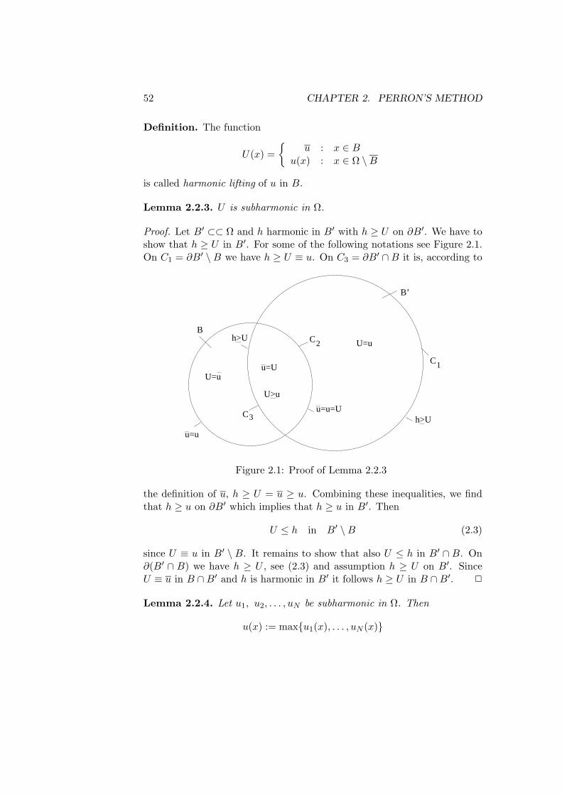
Lemma 2.2.3. U is subharmonic in Ω.
Proof. Let B′ ⊂⊂ Ω and h harmonic in B′ with h ≥ U on ∂B′. We have toshow that h ≥ U in B′. For some of the following notations see Figure 2.1.On C1 = ∂B′ \ B we have h ≥ U ≡ u. On C3 = ∂B′ ∩ B it is, according to
B’
h>U
C
U=u
h>UB
u=U
U>u
C
u=u
u=u=U
U=u
3
2
C1
Figure 2.1: Proof of Lemma 2.2.3
the definition of u, h ≥ U = u ≥ u. Combining these inequalities, we findthat h ≥ u on ∂B′ which implies that h ≥ u in B′. Then
U ≤ h in B′ \ B (2.3)
since U ≡ u in B′ \ B. It remains to show that also U ≤ h in B′ ∩ B. On∂(B′ ∩ B) we have h ≥ U , see (2.3) and assumption h ≥ U on B′. SinceU ≡ u in B ∩ B′ and h is harmonic in B′ it follows h ≥ U in B ∩ B′. 2
Lemma 2.2.4. Let u1, u2, . . . , uN be subharmonic in Ω. Then
u(x) := maxu1(x), . . . , uN (x)

2.2. SUBHARMONIC, SUPERHARMONIC FUNCTIONS 53
is also subharmonic in Ω, and if u1, . . . , uN are superharmonic, then u(x) :=minu1(x), . . . , uN (x) is superharmonic in Ω.
Proof. Exercise.
Definition. Let Ω be bounded and φ a bounded function on ∂Ω. A subhar-monic function u ∈ C(Ω) is called subfunction with respect to φ if u ≤ φ on∂Ω, and a superharmonic function u ∈ C(Ω) is called a superfunction withrespect to φ if u ≥ φ on ∂Ω.
Here u ≤ φ on ∂Ω means that
lim supy→x, y∈Ω, x∈∂Ω
u(y) ≤ φ(x).
Lemma 2.2.5. Suppose u is a subfunction and u a superfunction withrespect to φ. Then u ≤ u in Ω.
Proof. Lemma 2.2.2 and
lim supy→x, y∈Ω, x∈∂Ω
(u(y) − u(y)) = lim supy→x, y∈Ω, x∈∂Ω
(u(y) − φ(x) + φ(x) − u(y))
≤ lim supy→x, y∈Ω, x∈∂Ω
(u(y) − φ(x))
+ lim supy→x, y∈Ω, x∈∂Ω
(φ(x) − u(y))
≤ 0.
2
Remark. The set of subfunctions with respect to φ and the set of super-functions with respect to φ are not empty since constants ≤ inf∂Ω φ aresubfunctions and constants ≥ sup∂Ω φ are superfunctions.
SetSφ = v ∈ C(Ω) subharmonic in Ω : v ≤ φ on ∂Ω.
Theorem 2.2.1 (Perron, [19]). The function
u(x) := supv∈Sφ
v(x)
is harmonic in Ω.

54 CHAPTER 2. PERRON’S METHOD
Proof. (i) We have in Ω that
inf∂Ω
φ ≤ u(x) ≤ sup∂Ω
φ.
To show this inequality, let v ∈ Sφ, then v(x) ≤ φ(x) ≤ sup∂Ω φ on ∂Ω.Since the constant sup∂Ω φ is a superfunction with respect to φ and v is asubfunction with respect to φ we obtain from Lemma 2.2.5 the inequalityv(x) ≤ sup∂Ω φ, x ∈ Ω. Consequently u(x) ≤ sup∂Ω φ, x ∈ Ω. The otherside of the above inequality follows since the constant inf∂Ω φ is an elementof Sφ.
(ii) Let y ∈ Ω be fixed. Then there is a sequence vn ∈ Sφ with limn→∞ vn(y) =u(y). Let B = BR(y) ⊂⊂ Ω, R sufficiently small, and let Vn be the harmoniclifting of vn in B. Then
Vn ∈ Sφ, (2.4)
andlim
n→∞Vn(y) = u(y). (2.5)
Proof of (2.4): That Vn is subharmonic is the assertion of Lemma 2.2.3.Since Vn = vn on ∂B, we have Vn ≤ φ on ∂B.Proof of (2.5): We have
vn(y) ≤ Vn(y)
since vn = Vn on ∂B, Vn is harmonic in B and vn is superharmonic. Then
u(y) ≤ lim infn→∞
Vn(y).
On the other hand, since Vn ∈ Sφ, we have
Vn(y) ≤ supv∈Sφ
v(y) = u(y),
which implies thatlim sup
n→∞Vn(y) ≤ u(y).
(iii) For every function h harmonic in B we have,
supBρ(y)
|Dαh| ≤ C(ρ, R, α, n) supBR(y)
|h|, (2.6)
where 0 < ρ < R and the constant C is finite. This inequality is a conse-quence of Poisson’s formula for the solution of the Dirichlet problem in a

2.2. SUBHARMONIC, SUPERHARMONIC FUNCTIONS 55
ball, see [13, 10, 17], for example. Consequently for each fixed ρ, 0 ≤ ρ ≤ Rthere exists a subsequence Vnk
which converges uniformly in Bρ(y) to aharmonic function v. It follows that there is a subsequence of Vn, denotedalso by Vnk
, which converges uniformly on compact subsets of BR(0) to afunction v harmonic in BR(0). We have
v(x) ≤ u(x), x ∈ BR(y) (2.7)
since Vnk(x) ≤ u(x) on BR(y), see the definition of u(x). At the center y it
is, see (2.5),v(y) = u(y). (2.8)
(iv) Claim: v(x) = u(x), x ∈ B.Proof: If not, then there is a z ∈ B such that v(z) < u(z). Then there existsan u0 ∈ Sφ with v(z) < u0(z). Set
wk(x) := max(u0(x), Vnk(x)).
Let Wk be the harmonic lifting of wk in B. A subsequence of Wk convergesuniformly on each compact subset of B to a function w harmonic in B suchthat
v(x) ≤ w(x) ≤ u(x), x ∈ B = BR(y). (2.9)
These inequalities follow since wnk(x) ≤ Wnk
(x), wnk(x) ≥ Vnk
(x) andWnk
(x) ≤ u(x), where x ∈ B.Combining equation (2.8) and inequalities (2.9) we obtain
v(y) = w(y) = u(y). (2.10)
Thus the harmonic function v −w is less or equal zero in B and zero in theinterior point y ∈ B. The strong maximum principle implies that
v(x) = w(x), x ∈ B. (2.11)
According to the assumption we have for a z ∈ B
v(z) < u0(z).
On the other hand, see the definition of wn and Wn, if x ∈ B then
u0(x) ≤ wnk(x) ≤ Wnk
(x),
which implies thatu0(x) ≤ w(x), x ∈ B.

56 CHAPTER 2. PERRON’S METHOD
Summarizing, we have for the particular z under consideration the inequal-ities
v(z) < u0(z) ≤ w(z),
which is a contradiction to (2.11). 2
2.3 Boundary behaviour
One of the advantages of Perron’s method is that the boundary behaviourof solutions is separated from the existence problem.
Definition. A C(Ω)-function w = wξ is called a barrier at ξ ∈ ∂Ω relativeto Ω if
(i) w is superharmonic in Ω,
(ii) w > 0 in Ω \ ξ and w(ξ) = 0.
w is called a local barrier at ξ ∈ ∂Ω if there is a neighbourhood N of ξ suchthat w satisfies (i) and (ii) in Ω ∩N instead in Ω.
Let w be a local barrier at ξ ∈ ∂Ω, then we can define a barrier at ξ ∈ ∂Ωrelative to Ω as follows. Let B = BR(ξ), R > 0 sufficiently small such thatB ⊂⊂ N , see Figure 2.2. Set
.ξ
B
N
Ω
Γ
Figure 2.2: Definition of a local barrier
m = infN\B
w

2.3. BOUNDARY BEHAVIOUR 57
. We have m > 0, see assumption (ii) in the above definition.
Lemma 2.2.6. The function
w0(x) =
min(m, w(x)) : x ∈ Ω ∩ B
m : x ∈ Ω \ B
is a barrier at ξ relative to ∂Ω.
Proof. The property w0 ∈ C(Ω) follows since w0 = m on Γ = ∂B ∩ Ω. Ifnot, then there is an x0 ∈ Γ with w(x0) < m, which is a contradiction tothe definition of m. Now we will show that w0 is superharmonic in Ω. Thisfollows since
w0(x) =
w1 : x ∈ Ω ∩ B
w2 : x ∈ Ω \ B,
where w1(x) = min(m, w(x)), w2 = m and w1, w2 are superharmonic inΩ ∩ B and Ω \ B, respectively, and since w1 = w2 on Γ. To show this,consider a ball B′ ⊂⊂ Ω located as shown in Figure 2.3. Let h be harmonic
.ξ
Ω
B
B´
w =m0
Figure 2.3: A local barrier defines a barrier
in B′ with h ≤ w0 on ∂B′. We have to show that h ≤ w0 in B′. Sincew0 ≤ m on ∂1B
′ = ∂B′ ∩ B and w0 = m on ∂2B′ = ∂B′ \ ∂1B
′, we havew0 ≤ m on ∂B′. Thus the assumption h ≤ w0 on ∂B′ implies that h ≤ mon ∂B′. In particular h ≤ w0 in B′ \ B since w0 = m on B′ \ B. Finally wehave h ≤ w0 in B ∩ B′ since h ≤ w0 on B′ ∩ ∂B and on B ∩ ∂B′. We recallthat w0 = w1 in Ω∩B and w1 is superharmonic in Ω∩B, see Lemma 2.2.4.2
Definition. A boundary point is called regular if there exists a barrier atthat point.

58 CHAPTER 2. PERRON’S METHOD
Lemma 2.2.7. Let u be a harmonic function defined in Ω by the Perronmethod with boundary data φ. If ξ is a regular point af ∂Ω and if φ iscontinuous at ξ, then
limx→ξ,x∈Ω
u(x) = φ(ξ).
Proof. Fix ε > 0. Then there is a δ = δ(ε) > 0 such that |φ(x) − φ(ξ)| < εfor all x ∈ ∂Ω satisfying |x − ξ| < δ. Set M = sup∂Ω |φ|. Let w be a barrierat ξ. Then there is a k = k(ε) > 0 such that kw(x) > 2M if |x − ξ| ≥ δ.
Step 1. We will show that φ(ξ) + ε + kw(x) is a superfunction relative to φ.We recall that w ∈ C(Ω), w is superharmonic in Ω, w > 0 in Ω \ ξ andw(ξ) = 0. Then
φ(ξ) + ε + kw(x) ≥ φ(x)
on ∂Ω, since for x ∈ ∂Ω with |x − ξ| ≥ δ we have
φ(ξ) + ε + kw(x) ≥ φ(ξ) + ε + 2M
≥ φ(x),
and for x ∈ ∂Ω with |x − ξ| < δ we have
φ(x) − φ(ξ)| ≤ ε
since |φ(x) − φ(ξ)| ≤ ε if x ∈ ∂Ω ∩ Bδ(ξ) and kw(x) ≥ 0.
Step 2. Since
u(x) = supv∈Sφ
v(x)
and φ(ξ) − ε − kw(x) is a subfunction relative to φ, we have
φ(ξ) − ε − kw(x) ≤ u(x)
in Ω. The function φ(ξ) + ε + kw(x) is a superfunction relative to φ, seeStep 1. Concequently,
v(x) ≤ φ(ξ) + ε + kw(x)
for all v ∈ Sφ, see Lemma 2.2.5. This inequality implies that
u(x) ≤ φ(ξ) + ε + kw(x).
2.3. BOUNDARY BEHAVIOUR 59
Summarizing, we get
|u(x) − φ(ξ)| ≤ ε + kw(x).
Since limx→ξ,x∈Ω w(x) = 0, we obtain finally
limx→ξ,x∈Ω
u(x) = φ(ξ).
2
Theorem 2.2.2. Let Ω ⊂ Rn be bounded and connected. Then the Dirichlet
problem 4u = 0 in Ω, u = φ on ∂Ω, where φ ∈ C(∂Ω) is given, is solvableif and only if the boundary points are all regular.
Proof. (i) Assume all points of ∂Ω are regular points. Then the assertionfollows from previous Lemma 2.2.7.(ii) Assume the Dirichlet problem is solvable for all continuous φ ∈ C(∂Ω).Set φ(x) := |x − ξ| and consider the Dirichlet problem with the boundarycondition u(x) = φ(x) on ∂Ω. Let uξ(x) be the solution, then uξ(x) is abarrier at ξ. Consequently all boundary points are regular.
2
2.3.1 Examples for local barriers
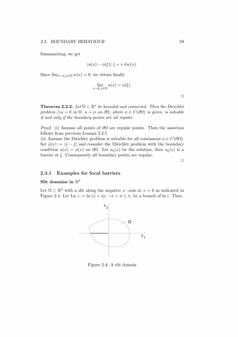
Slit domains in R2
Let Ω ⊂ R2 with a slit along the negative x−axis at x = 0 as indicated in
Figure 2.4. Let Ln z := ln |z| + iφ, −π < φ ≤ π, be a branch of ln z. Then
Ω
x
x
1
2
Figure 2.4: A slit domain
60 CHAPTER 2. PERRON’S METHOD
w := −Re
(
1
Lnz
)
= − ln r
ln2 r + φ2
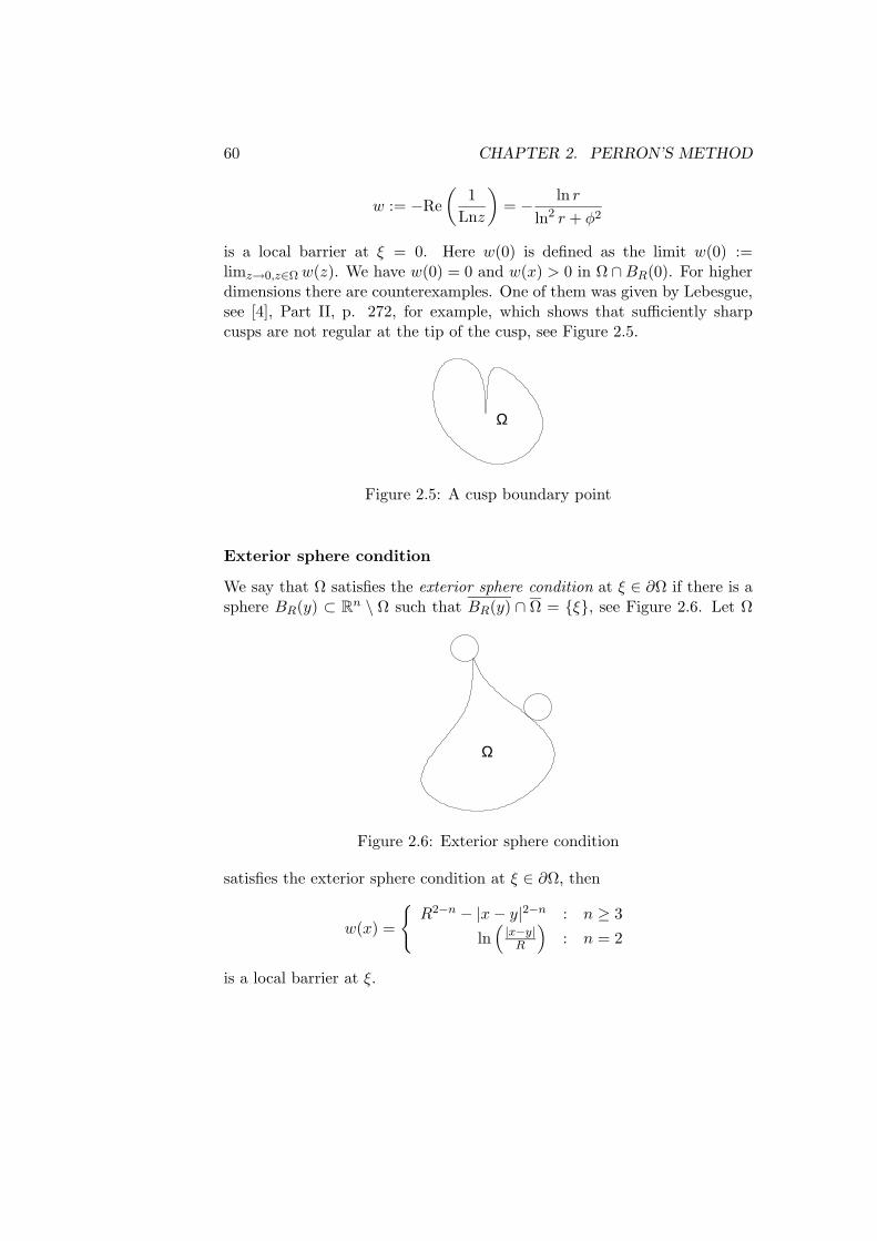
is a local barrier at ξ = 0. Here w(0) is defined as the limit w(0) :=limz→0,z∈Ω w(z). We have w(0) = 0 and w(x) > 0 in Ω ∩ BR(0). For higherdimensions there are counterexamples. One of them was given by Lebesgue,see [4], Part II, p. 272, for example, which shows that sufficiently sharpcusps are not regular at the tip of the cusp, see Figure 2.5.
Ω
Figure 2.5: A cusp boundary point
Exterior sphere condition
We say that Ω satisfies the exterior sphere condition at ξ ∈ ∂Ω if there is asphere BR(y) ⊂ R
n \ Ω such that BR(y) ∩ Ω = ξ, see Figure 2.6. Let Ω
Ω
Figure 2.6: Exterior sphere condition
satisfies the exterior sphere condition at ξ ∈ ∂Ω, then
w(x) =
R2−n − |x − y|2−n : n ≥ 3
ln(
|x−y|R
)
: n = 2
is a local barrier at ξ.

2.3. BOUNDARY BEHAVIOUR 61
Exterior cone condition
We say that Ω satisfies an exterior cone condition at ξ ∈ ∂Ω if there isa finite circular cone C with the vertex at ξ such that K ∩ Ω = ξ, seeFigure 2.7. Let ξ be the origin and assume the exterior cone property is
Ω
Figure 2.7: Exterior cone condition
satisfied at ξ ∈ ∂Ω. Then we can find a positive constant λ and a positivefunction f(θ), where θ is the polar angle, such that
w = rλf(θ),
r = |x|, is a local barrier at ξ.
Two-dimensional domains. Here we find λ and f(θ) as follows. Let
C ⊂ (r, θ) : r > 0, −α < θ < α,
see Figure 2.8 Introducing polar coordinates (r, θ), where
x1 = r sin θ, x2 = r cos θ,
we have
w(x) = W (r, θ) := w(r cos θ, r sin θ)
4w =1
r
∂
∂r(rWr) +
1
r2Wθθ.
Consider the ansatzW (r, θ) = rλ cos(µθ),
where λ and µ are positive constants, then
4w = rλ−2(λ2 − µ2) cos(µθ).

62 CHAPTER 2. PERRON’S METHOD
Ω
θ
x
x
1
C
2
Figure 2.8: Local barrier, R2
Consequently 4w ≤ 0 on C if λ ≤ µ and |µθ| ≤ π/2 for all θ satisfyingα < θ < 2π − α (0 < α < π/2).
Then w > 0 if r > 0 and α < θ < 2π − α. Thus w is a local barrier atthe origin if we choose λ = µ with a sufficiently small positive µ.
Higher dimensional case. Let M ⊂ ∂B1(O) be the manifold as indicated inFigure 2.9. Consider the eigenvalue problem
−4′v = ν2v in Mv = 0 on ∂M,
where 4′ is the Laplace-Beltrami differential operator on the unit sphere.We recall that in the two-dimensional case
4′ =∂2
∂θ2
and in the three-dimensional case
4′ =1
sin θ
∂
∂θ
(
sin θ∂
∂θ
)
+1
sin2
∂2
∂φ2.
For the definition of the Laplace-Beltrami operator see for example [2]and for n-dimensional polar coordinates see [7], Part III, pp. 395, for exam-ple.

2.4. GENERALIZATIONS 63
Ω
θ
xn
0M
Figure 2.9: Local barrier, Rn
Let ν1 be the first eigenvalue of the above eigenvalue problem. It is knownthat ν1 is positive, a simple eigenvalue and the associated eigenfunction v1
has no zero in M. Thus, we can assume that v1 > 0 in M. Set
W = Arκv1 ≡ w(x)
where A and κ are positive constants. Then w > 0 in Rn \ C and
4w = Arκ−2v1 (κ(κ − 1) + (n − 1)κ − α1) ,
where
α1 = −n − 2
2+
√
(
n − 2
2
)2
+ ν21 .
Consequently we have 4w ≤ 0 in Rn\C, provided κ > 0 is sufficiently small.
2.4 Generalizations
Perron’s method can be applied to the Dirichlet problem for a more generalclass of linear elliptic equations of second order, see for example [10], pp. 102.The previous discussion in the case of the Laplace equation showes that weneed a strong maximum principle, the existence of solutions of the Dirichletproblem on a ball with continuous boundary data and some estimates forthe derivatives. Then we are able to prove the existence of a solution of
64 CHAPTER 2. PERRON’S METHOD
the equation in the given domain. The problem of the boundary behaviourrequires an additional discussion.

2.5. EXERCISES 65
2.5 Exercises
1. Let Ω ⊂ Rn be a connected domain. Consider the eigenvalue problem
−4u = λu in Ω
u = 0 on ∂Ω.
Suppose λ0 ≥ 0 is an eigenvalue and u0 ∈ C2(Ω)∩C(Ω) an associatedeigenfunction satisfying u0(x) ≥ 0 in Ω. Show that u0(x) > 0 in Ω.
2. Prove the second corollary to Theorem 2.1.1.
3. Prove Lemma 2.2.4.

66 CHAPTER 2. PERRON’S METHOD

Chapter 3
Maximum principles
Maximum principles provide powerful tools for linear and nonlinear ellipticequations of second order. We consider linear equations.
3.1 Basic maximum principles
Set
Mu =n
∑
i,j=1
aij(x)Diju +n
∑
i=1
bi(x)Diu
Lu = Mu + c(x)u,
where ai,j , bi and c are real and defined on a simply connected domainΩ ⊂ R
n. We assume aij = aji. Let λ(x) be the minimum of the eigenvaluesof the symmetric matrix defined by the coefficients aij and let Λ(x) be themaximum of these eigenvalues.
Definition. L is called elliptic in Ω if λ(x) > 0 in Ω. L is said to be strictlyelliptic in Ω if λ(x) ≥ λ0 > 0 in Ω, where λ0 is a constant. An elliptic L iscalled uniformly elliptic if Λ/λ is bounded in Ω.
In the following we suppose that L is at least elliptic and for each i
supx∈Ω
|bi(x)|λ(x)
< ∞. (3.1)
Theorem 3.1.1 (Weak maximum principle). Let L be elliptic in the boundeddomain Ω. Assume a function u ∈ C2(Ω)∩C(Ω) satisfies Mu ≥ 0 (Mu ≤ 0)in Ω. Then the supremum (infimum) of u on Ω is achieved on ∂Ω.
67

68 CHAPTER 3. MAXIMUM PRINCIPLES
Proof. Assume initially that Mu > 0 in Ω. Then u cannot achieves an inte-rior maximum since ∇u(x0) = 0 at this point where u achives its maximum,and since the matrix D2u(x0) = [Diju(x0)] is nonpositive (necessary condi-tion of second order). It follows that, see an exercice in [17], for example,
Mu(x0) =n
∑
i,j=1
aij(x0)Diju(x0) ≤ 0
since the matrix [aij(x0)] is nonnegative (even positive) by assumption. Thisinequality is a contradiction to our assumption.
For a positive sufficiently large constant γ we calculate
Meγx1 = (γ2a11 + γb1)eγx1
≥ λ(γ2 − γc1)eγx1 > 0.
We recall that a11 ≥ λ and |b1|/λ ≤ c1, where c1 is a positive constant, seeassumption (3.1). Consequently for any ε > 0 we have in Ω
M (u + εeγx1) > 0.
Using the above result, we conclude that
supΩ
(u + εeγx1) = sup∂Ω
(u + εeγx1) .
Letting ε → 0, we obtainsupΩ
u = sup∂Ω
u.
2
The next theorem is the strong maximum principle. It follows from theboundary point lemma due to E. Hopf [11]. The proof of this lemma needsthe previous weak maximum principle. The strong maximum principle isthe essential tool to show existence of a solution of the Dirichlet problemvia Perron’s method.
Lemma 3.1.1 (E. Hopf, 1952). Let L be uniformly elliptic. Assume u ∈C2(Ω) satisfies Mu ≥ 0 in Ω. Let x0 ∈ ∂Ω and suppose that(i) u is continuous at x0,(ii) u(x0) > u(x) for all x ∈ Ω ∩ Ba(x0) for an a > 0,(iii) ∂Ω satisfies the interior sphere condition at x0.Then the outer normal derivative of u at x0, if it exists, satisfies
∂u
∂ν(x0) > 0.

3.1. BASIC MAXIMUM PRINCIPLES 69
Proof. Let B = BR(y) be the ball related to the interior sphere condition,see Figure 3.1. Consider the function
.
.
.
x
x
y
BR
(y)
ν
ρ
0
Figure 3.1: Proof of Hopf’s boundary point lemma
v(x) = e−αr2 − e−αR2
,
where r = |x − y| > ρ and α is a positive constant which we will determinelater. A calculation leads to
Mv = e−αr2(
4α2n
∑
i,j=1
aij(xi − yi)(xj − yj)
−2α(
n∑
i=1
aii +n
∑
i=1
bi(xi − yi))
)
≥ e−αr2(
4α2λ(x)r2 − 2α(
n∑
i=1
aii + |b|r)
)
,
where b = (b1, . . . , bn). Since by assumption aii/λ and |b|/λ are bounded,we may choose α large enough such that Mv ≥ 0 in the annular domainA := BR(y) \ Bρ(y). Since u(x) − u(x0) < 0 on ∂Bρ(y) there is a constantε > 0 such that u(x) − u(x0) + εv(x) ≤ 0 on ∂Bρ(y). This inequality is

70 CHAPTER 3. MAXIMUM PRINCIPLES
also satisfied on ∂BR(y) by assumption on u and since v = 0 on ∂BR(y).We have M
(
u(x)− u(x0) + εv(x))
= Mu + εMv. Then the weak maximumprinciple implies that u − u(x0) + εv ≤ 0 in A. Thus
u(x0) − u(x) ≥ −ε(
v(x0) − v(x))
,
where x ∈ A and on the line defined by x0 and ν. It follows
∂u
∂ν(x0) ≥ −εV ′(R),
provided the normal derivative exists. Here is
V (r) = e−αr2 − e−αR2
.
2
Remark. If the normal derivative does not exist, then
lim infx→x0
u(x0) − u(x)
|x0 − x| > 0,
where the angle between x0−x and the exterior normal ν is less then (π/2)−δfor a fixed δ > 0.
Corollary. Suppose that ∂Ω satisfies the interior sphere condition at x0 ∈∂Ω, u ∈ C2(Ω)∩C(Ω) satisfies Lu ≥ 0 and u(x0) > u(x) in Ω∩U , where Uis a neighbourhood of x0. If additionally c ≤ 0 in Ω ∩ U and u(x0) > 0 then∂u/∂ν(x0) > 0, provided the normal derivative exists.
Proof. Mu = Lu − cu ≥ 0 in Ω ∩ V, where V is a neighbourhood of x0. 2
In generalization to the strong maximum principle for 4 we have
Theorem 3.1.2 (Strong maximum principle). Let L be uniformly elliptic.Assume u ∈ C2(Ω)∩C(Ω) satisfies Mu ≥ 0 (Mu ≤ 0) in a connected domainΩ, not necessarily bounded. Then if u achieves its supremum (infimum) inthe interior of Ω, u is a constant.
Proof. Consider the case of a maximum. Assume u is not constant andachieves its maximum m in the interior of Ω. Set Ω1 = x ∈ Ω : u(x) = mand Ω2 = x ∈ Ω : u(x) < m. By assumption Ω1 is not empty. We willshow that Ω1 is open. Then Ω2 = ∅ since we suppose that Ω is connected.

3.1. BASIC MAXIMUM PRINCIPLES 71
Let x1 ∈ Ω1. Consider a ball B = B2ρ0(x1) ⊂⊂ Ω. If Ω1 is not open, then
there is an x2 ∈ Bρ0(x1) such that u(x2) < m. Consequently there is a ball
Bρ(x2), where 0 < ρ ≤ |x2 − x1|, and u(x) < m in Bρ(x
2) and there is anx3 ∈ ∂Bρ(x
2) such that u(x3) = m. See Figure 3.2 for notations. Hopf’s
.
..
2
x
x
x3
2
1ρ
0
ρ0
Figure 3.2: Proof of the strong maximum principle
lemma says that (∂u/∂ν) (x3) > 0, where ν is the exterior normal derivativeon x3 ∈ ∂Bρ(x
2) at u(x3) which is a contradiction to the fact that u attendsan interior maximum at x3. 2
In many cases the assumption c ≡ 0 in Ω is not satisfied. If c(x) ≤ 0 inΩ, then we have the following corollary to the previous theorem. If c(x) ispositive on a subset of Ω, then the situation is more complicated. In thiscase one studies an associated eigenvalue problem.
Corollary. Let Ω be a connected domain, not necessarily bounded. SupposeL is uniformly elliptic and c(x) ≤ 0 in Ω. Assume u ∈ C2(Ω)∩C(Ω) satisfiesLu ≥ 0 (Lu ≤ 0). If u achieves its positive supremum (negative infimum)in the interior of Ω then u is a constant.
Proof. Consider the case of a maximum. Set m = supΩ u(x) and Ω1 = x ∈Ω : u(x) = m, Ω2 = x ∈ Ω : u(x) < m. By assumption Ω1 is not empty.We show that Ω1 is an open set. Let x1 ∈ Ω1. Then there is ball Bρ(x
1) ⊂ Ω

72 CHAPTER 3. MAXIMUM PRINCIPLES
where u is nonnegative. Thus
Mu ≡ Lu − c(x)u ≥ 0
in Bρ(x1). The above strong maximum principle (Theorem 3.1.2) says that
u(x) = m for all x ∈ Bρ(x1).
2
From this corollary follows a result important for many applications:
Theorem 3.1.3 (Comparison principle). Let Ω be a bounded and connecteddomain. Suppose that L is uniformly elliptic and c(x) ≤ 0 in Ω. Assumeu, v ∈ C2(Ω) ∩ C(Ω) and satisfy Lu ≥ Lv in Ω and u ≤ v on ∂Ω. Thenu ≤ v in Ω.
Proof. Set w = u−v. Then Lw ≥ 0 in Ω and w ≤ 0 on ∂Ω. From the abovecorollary we see that w can not achieve a positive maximum in Ω. 2
3.1.1 Directional derivative boundary value problem
As an application of the previous corollary we consider a generalization ofthe Neumann problem. Let Ω ⊂ R
n be a bounded and connected domain,and assume ∂Ω is sufficiently smooth. Consider
Lu = f, in Ω (3.2)
∂u
∂α= φ on ∂Ω, (3.3)
where f, φ are given and sufficiently regular, and the direction α is nottangential on ∂Ω at each point of ∂Ω, see Figure 3.3.
ν
x0
α
t
Figure 3.3: Directional derivative boundary value problem
Proposition 3.1.1. Suppose that c ≤ 0 in Ω and let u1, u2 ∈ C2(Ω)∩ C1(Ω)are solutions of (3.2), (3.3). Then u1 − u2 ≡ const. in Ω.

3.1. BASIC MAXIMUM PRINCIPLES 73
Proof. Set u = u1 − u2, then Lu = 0 in Ω and ∂u/∂α = 0 on ∂Ω. Supposethat u is not constant, then we can assume maxΩ u > 0. This maximumis achieved at x0 ∈ ∂Ω and u(x0) > u(x) for all x ∈ Ω, see the corollaryto the strong maximum principle. For the tangential derivative we have(∂u/∂t)(x0) = 0, and the assumption implies that (∂u/∂α)(x0) = 0. Thus
(∂u/∂ν)(x0) = a(x0)(∂u/∂t)(x0) + b(x0)(∂u/∂α)(x0)
= 0,
which is a contradiction to the corollary to the Hopf boundary point lemmawhich says that ∂u/∂ν > 0 at x0. 2
3.1.2 Behaviour near a corner
Set Lu =∑2
i,j=1 aij(x)uxixjand consider the Dirichlet problem
Lu = f in Ω (3.4)
u = 0 on ∂Ω, (3.5)
where f is given. Suppose that the boundary of Ω ⊂ R2 has a corner.
Without loss of generality we suppose that the corner is the origin. SetΩρ = Ω ∩ Bρ(0). Then we assume that there is a ρ > 0 such that in Ωρ
we have aij = aji, L is uniformly elliptic, aij ∈ Cα(Ωρ). An appropriaterotation with center at the origin and a streching of the axis transforms(3.4), (3.5) into a Dirichlet problem where aij(0, 0) = δij . Here we denotethe transformed coefficients aij(C
−1y) and the transformed right hand sidef(C−1y) by aij and f , resp., and y by x. The new domain is denoted by Ωagain. The new interior angle ω can be calculated from the original interiorangle γ and the original coefficients [aij(0, 0)], see an exercice. After thismapping we arrived at the problem
Lu = 4u +2
∑
i,j=1
(aij(x) − δij)uxixj= f in Ωρ (3.6)
u = 0 on ∂Ω ∩ Ωρ, (3.7)
where|aij(x) − δij | ≤ c|x|α.
Suppose that Ωρ is contained in a domain, see Figure 3.4, defined by 0 <r < ρ and θ1(ρ) ≤ θ ≤ θ2(ρ), where r = (x2
1 + x22)
1/2. Set
ω = ω(ρ) = θ2(ρ) − θ1(ρ)
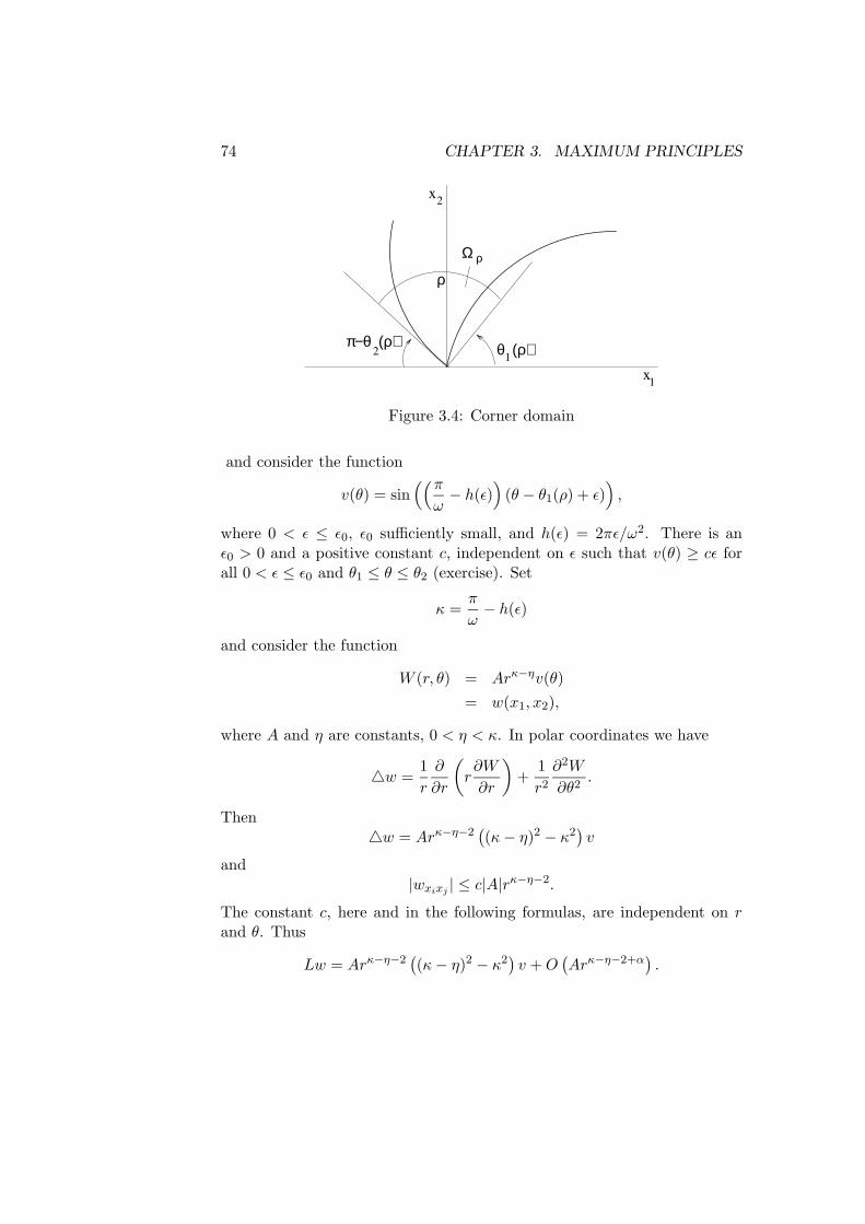
74 CHAPTER 3. MAXIMUM PRINCIPLES
π−θ (ρ)
Ω
θ (ρ)1
2
ρ
ρ
x1
2x
Figure 3.4: Corner domain
and consider the function
v(θ) = sin((π
ω− h(ε)
)
(θ − θ1(ρ) + ε))
,
where 0 < ε ≤ ε0, ε0 sufficiently small, and h(ε) = 2πε/ω2. There is anε0 > 0 and a positive constant c, independent on ε such that v(θ) ≥ cε forall 0 < ε ≤ ε0 and θ1 ≤ θ ≤ θ2 (exercise). Set
κ =π
ω− h(ε)
and consider the function
W (r, θ) = Arκ−ηv(θ)
= w(x1, x2),
where A and η are constants, 0 < η < κ. In polar coordinates we have
4w =1
r
∂
∂r
(
r∂W
∂r
)
+1
r2
∂2W
∂θ2.
Then4w = Arκ−η−2
(
(κ − η)2 − κ2)
v
and|wxixj
| ≤ c|A|rκ−η−2.
The constant c, here and in the following formulas, are independent on rand θ. Thus
Lw = Arκ−η−2(
(κ − η)2 − κ2)
v + O(
Arκ−η−2+α)
.

3.1. BASIC MAXIMUM PRINCIPLES 75
Suppose that the constant A is positive, then from the above considerationsit follows that for given δ > 0, 0 < δ ≤ δ0, δ0 sufficiently small, there arepositive constants c(δ) and ρ = ρ(δ) such that
Lw ≤ −Ac(δ)r(π/ω)−δ−2
in Ωρ.
Proposition 3.1.2. Assume the right hand side f of (3.4) satisfies
|f | ≤ cr(π/ω)−2−δ+τ
in Ωρ0, ρ0 > 0, for a τ > 0. Assume u ∈ C2(Ωρ0
) and supΩρ0|u(x)| < ∞.
Then for given (small) ε > 0 there exists positive constants c(ε) and ρ(ε) > 0such that
|u| ≤ c(ε)|x|(π/ω)−ε
in Ωρ(ε).
Proof. We have Lw ≤ Lu in Ωρ and w ≥ u on ∂Ωρ, provided ρ > 0 issufficiently small. 2
Remark. The additional assumption that u remains bounded up to thecorner is essential for the previous proposition since there exists also solu-tions which are unbounded near the corner. An example is the boundaryvalue problem 4u = 0 in Ωα, u = 0 on ∂Ωα, where Ωα is the sector definedby r > 0 and 0 < θ < α, where 0 < α < 2π. Solutions are given by
u(x) = rπk/α sin ((π/α)kθ) ,
where k ∈ ±1,±2, . . .. For a class of quasilinear nonuniformly boundaryvalue problems the behaviour of the solution near the corner does not re-quire such an additional assumption near the boundary, see [8, 16, 3, 18].The behaviour follows from the problem itself. The reason for this strikingdifference is that essential information is lost through the linearization.
Remark. Asymptotic expansions near a corner yield more precise be-haviour near the corner, see [15] for a class of uniformly quasilinear ellipticDirichlet problems. In general, the expansion, depends on the solution con-sidered, in contrast to some nonuniformly problems, see [16].

76 CHAPTER 3. MAXIMUM PRINCIPLES
3.1.3 An apriori estimate
Consider for given bounded functions f , Φ defined on Ω and on ∂Ω, respec-tively, the Dirichlet problem
Lu =n
∑
i,j=1
aij(x)Diju +n
∑
i=1
bi(x)uxi+ c(x) = f(x) in Ω (3.8)
u = Φ on ∂Ω (3.9)
where ai,j , bi and c are real and defined on a simply connected and boundeddomain Ω ⊂ R
n. We assume aij = aji, L is strictly elliptic and
supΩ
|bi(x)| < ∞
for every i = 1, . . . , n. Let K be a bound of b1 and set
α =1
λ0
(
K + (K2 + 4λ0)1/2
)
, (3.10)
where the positive constant λ0 is a lower bound of the minimum of theeigenvalues of the matrix [aij(x)]. Set d = diam Ω.
Proposition 3.1.3. Suppose that c(x) ≤ 0 in Ω and let u ∈ C2(Ω) ∩ C(Ω)be a solution of (3.8), (3.9). Then
supΩ
|u| ≤ sup∂Ω
|Φ| +(
eαd − 1)
supΩ
|f |.
Proof. Suppose that Ω is contained in the strip defined by 0 ≤ x1 ≤ d.Consider the function
g(x) = eαd − eαx1 ,
where α is positive constant which will be determined later. We have g(x) ≥0 if x ∈ Ω. We get
Lg = −(a11α2 + b1α)eαx1 + cg
≤ (λ0α2 + Kα)eαx1
≤ −eαx1
≤ −1,
provided that α is large enough. We can choose α given by (3.10). Set
h = sup∂Ω
|Φ| + g(x) supΩ
|f |.
3.2. A DISCRETE MAXIMUM PRINCIPLE 77
Then
Lh = Lg supΩ
|f | + c sup∂Ω
|Φ|
≤ − supΩ
|f |.
We recall that c ≤ 0 on Ω. Summarizing, we have
Lh ≤ − supΩ
|f | in Ω
h ≥ supΩ
|Φ| on ∂Ω.
Set v = u − h, then
Lv = f − Lh ≥ f + supΩ
|f | ≥ 0 in Ω
v = Φ − sup∂Ω
|Φ| ≤ 0 on ∂Ω.
The comparison principle says that v ≤ 0 in Ω. The same argument leadsto the inequality u ≥ −h in Ω if we set v = −u − h. Then
Lv = −f − Lh ≥ −f + supΩ
|f | ≥ 0 in Ω
v = −Φ − h ≤ −Φ − sup∂Ω
|Φ| ≤ 0 on ∂Ω.
2
3.2 A discrete maximum principle
To simplify the presentation we consider here a subclass of elliptic boundaryvalue problems in a domain Ω ∈ R
2, see [12], pp. 458, for example. Set
Mu = 4u + b1(x, y)ux + b2(x, y)uy.
Suppose that there is a constant K such that
supΩ
(|b1(x, y)| + |b2(x, y)|) ≤ K. (3.11)
Let
Lu = Mu + c(x, y)u,

78 CHAPTER 3. MAXIMUM PRINCIPLES
where c(x, y) is defined on Ω. Then we consider for given f defined on Ω,and Φ defined on ∂Ω, the Dirichlet problem
Lu = f in Ω (3.12)
u = Φ on ∂Ω. (3.13)
Let h > 0 be a (small) constant. Then we define an associated differenceoperator to Mu by
Mhu =u(x + h, y) + u(x − h, y) + u(x, y + h) + u(x, y − h) − 4u(x, y)
h2
+b1(x, y)u(x + h, y) − u(x − h, y)
2h+ b2(x, y)
u(x, y + h) − u(x, y − h)
2h.
We have limh→0 Mhu = Mu on every compact subdomain of Ω, providedu ∈ C2(Ω).
Set P0 = (x, y) and assume P0 ∈ Ω. The four points P01 = (x + h, y),P02 = (x, y+h), P03 = (x−h, y), P04 = (x, y−h) are called h-neighbourhoodof P0 or a star around P0. Consider the intersection of Ω with an h-net Nh
of R2 defined by
Nh(x, y) = (x + lh, y + kh) ∈ R2 : k, l = 0,±1,±2, . . .,
where (x, y) ∈ R2 is given. Let Ωh be the set of the points Pi of Ω∩Nh such
that each point of the star associated to Pi are contained in Ω. The set ofall star points not in Ωh is denoted by ∂Ωh, see Figure 3.5. Then we define
Figure 3.5: Definition of Ωh and ∂Ωh
Ωh = Ωh ∪ ∂Ωh.
3.2. A DISCRETE MAXIMUM PRINCIPLE 79
Suppose that Ωh is connected in the sense that for given P, R ∈ Ωh
there exists points Q1, Q2, . . . , Qs ∈ Ωh, where Q1 = P and Qs = R, suchthat Qj is a point of the h-neighbourhood of Qj−1, j = 1, . . . , s + 1. Weassume that h > 0 is sufficiently small such that
hK < 1. (3.14)
Theorem 3.2.1. Let u be defined on Ωh. Suppose that Mhu ≥ 0 in Ωh andu attends its maximum in Ωh. Then u is constant on Ωh.
Proof. Let Pi ∈ Ωh. From the definition of Mhu and the assumption Mhu ≥0 we obtain that
u(Pi) ≤4
∑
j=1
λiju(Pij),
where Pij are the points of the h-neighbourhood of Pi and
λi1 =1
4
(
1 +hb1(Pi)
2
)
, λi2 =1
4
(
1 +hb2(Pi)
2
)
λi3 =1
4
(
1 − hb1(Pi)
2
)
, λi4 =1
4
(
1 − hb2(Pi)
2
)
.
We have∑4
j=1 λij = 1 and, see (3.14), λij > 0. Assume
m := maxΩh
u(x) = u(Pi).
Then u = m in all points of the h-neighbourhood of Pi. Since Ωh is con-nected, the theorem is shown. 2
Set Lhu = Mhu + c(x)u. The following corollary is the discrete version ofthe corollary to the above Theorem 3.2.
Corollary. Suppose that c(x) ≤ 0 on Ωh and u defined on Ωh satisfiesLhu ≥ 0 on Ωh. Then if u achieves its nonnegative supremum m in Ωh, uis constant on Ωh.
Proof. Set Ωh,1 = x ∈ Ωh : u(x) = m and Ωh,2 = x ∈ Ωh : u(x) < m.By assumption Ωh,1 is not empty. The set Ωh,1 is open in the sense that ifPi ∈ Ωh,1 then u(Pil) = m for every point Pil, l = 1, 2, 3, 4, of the associated
80 CHAPTER 3. MAXIMUM PRINCIPLES
star to Pi. This follows from the inequality
u(Pi) ≤3
∑
j=1
λiju(Pij) +h2
4c(Pi)u(Pi).
Thus u = m on Ωh since Ωh is connected by assumption. 2
From this corollary it follows
Theorem 3.2.2 (Comparison principle). Let Ωh be a bounded and connecteddomain. Suppose that c(x) ≤ 0. Assume u, v are defined on Ωh and satisfyLhu ≥ Lhv in Ωh and u ≤ v on ∂Ωh. Then u ≤ v on Ω.
Proof. Set w = u − v. Then Lhw ≥ 0 in Ωh and w ≤ 0 on ∂Ωh. From theabove corollary we see that w can not achieve a nonnegative maximum inΩ. 2
Suppose that Ωh is bounded and connected. We consider the discrete Dirich-let problem
Lhu = f in Ωh (3.15)
u = Φ on ∂Ωh, (3.16)
where f is defined in Ωh and Φ on ∂Ωh. Assume c ≤ 0 and h is sufficientlysmall such that the inequality (3.14) is satisfied.
Corollary. There exists a unique solution of the discrete Dirichlet prob-lem (3.15), (3.16).
Proof. The Dirichlet problem defines a linear system of N equations in Nunknowns. From the comparison principle it follow that there is at mostone solution. From the linear algebra it is known that uniqueness impliesexistence. 2
Proposition 3.2.1 (Apriori etimate). Assume u is a solution of the discreteDirichlet problem (3.15), (3.16), where c(x) ≤ 0. Then
maxΩh
|u| ≤ max∂Ωh
|Φ| + c maxΩh
|f |,
where the constant c is independent of u and h, and 0 < h < h0, h0 suffi-ciently small, see the following proof for an explicit h0.

3.2. A DISCRETE MAXIMUM PRINCIPLE 81
Proof. The proof is the same as the proof of the apriori estimate of Theo-rem 3.4. Concerning notations in the following formula see the proof of thistheorem. For a sufficiently large α we have
Lh
(
eαd − eαx)
= −α2eαx
(
sinh(αh/2)
αh/2
)2
−b1(x)αeαx sinh(αh)
αh+ c(x)
(
eαd − eαx)
≤ −eαx
(
α2
(
sinh(αh/2)
αh/2
)2
+ b1αsinh(αh)
αh
)
.
Suppose that αh ≤ 1, then
Lh
(
eαd − eαx)
≤ −eαx(
α2 − Kα cosh(1))
≤ −1,
if we take an α which satisfies
α ≥ (K/2) cosh(1) +
√
((K/2) cosh(1))2 + 1.
We recall that we assume that Ω is bounded and is contained in the strip0 < x1 < d, where d is the diameter of Ω. 2
The following result says that the solution of the discrete Dirichlet problemis an approximation of the solution of the original problem, provided thatthis solution is sufficiently smooth,
Corollary. Suppose that u ∈ C3(Ω) is a solution of the continuous Dirichletproblem (3.12), (3.13), where c(x) ≤ 0 and Φ is defined on a boundarystrip and is in C1 in the closed strip. Let uh be a solution of the discreteproblem (3.15), (3.16). Then
maxΩh
|u(x) − uh(x)| ≤ ch,
where the constant c is independent on h < h0, h0 sufficiently small.
Proof. Here we make the additional assumption that ∂Ωh ⊂ ∂Ω, see Fig-ure 3.5 for an example. The proof of the general case is left as an exercise.The assumption on u implies that
|Lhu − Lu| ≤ ch. (3.17)
82 CHAPTER 3. MAXIMUM PRINCIPLES
Let U be defined on Ωh. Then we have from the above apriori estimate that
maxΩh
|U | ≤ max∂Ωh
|U | + c maxΩh
|LhU |.
Set U = u − uh, then
maxΩh
|u − uh| ≤ c maxΩh
|Lhuh − Lhu|
since u − uh = 0 on ∂Ωh. Finally, we have on Ωh that
Lhuh − Lhu = Lhuh − Lu + Lu − Lhu
= Lu − Lhu
since Lhuh = f and Lu = f on Ωh. Then the estimate of the corollaryfollows from the estimate (3.17). 2

3.3. EXERCISES 83
3.3 Exercises
1. Let Ω ⊂ Rn be a bounded domain and assume u ∈ C(Ω) and
supΩ
(u + εeγx1) = sup∂Ω
(u + εeγx1)
for each ε. Show thatsupΩ
u = sup∂Ω
u.
2. Let [aij ] be a real regular symmetric matrix in Rn. Find a regular
Matrix C in Rn such that
n∑
i,j=1
aijuxixj=
n∑
i=1
Uyiyi,
where U(y) := u(C−1y).
Hint: Let Z1,Z2 be an orthonormal system of eigenvectors to [aij ] tothe eigenvalues λ1, λ2, respectively. Set B = (Z1,Z2), then
C =
(
1/√
λ1 00 1/
√λ2
)
BT .
3. Let γ be the interior angle of a sector with its corner at the origin inR
2. Calculate the interior angle ω of the sector transformed by theabove mapping.
4. Let u ∈ C1(Ω) ∩ C2(Ω) be a solution of
div∇u
√
1 + |∇u|2= f inΩ
u = Φ on ∂Ω,
where Ω ∈ R2 and f, Φ are given. Suppose the origin is a corner of
Ω with interior angle γ, 0 < γ < π. Show that ω, see the previousexercise, is the opening angle of the surface S defined by z = u(x1, x2),over the origin, see Figure 3.6.
Hint:
div∇u
√
1 + |∇u|2=
2∑
i,j=1
aij(x)uxixj,

84 CHAPTER 3. MAXIMUM PRINCIPLES
z
ω
γ
S
Ω
Figure 3.6: Transformed opening angle
where
aij =1
(1 + |∇u|2)3/2
(
δij −uxi
uxj
1 + |∇u|2)
.
5. Let Ωα be the sector in R2 defined by r > 0 and 0 < θ < α, where
0 < α < 2π. Set Ωα,ρ = Ωα ∩ Bρ(0). Suppose that u ∈ C2(Ωα,ρ \ 0)and supΩα,ρ
|u| < ∞ is a solution of 4u = 0 in Ωα,ρ, u = 0 on (∂Ωα ∩Bρ(0)) \ 0.Show that there is a constant c such that
|u| ≤ c|x|π/α
in Ωα,ρ.
Hint: Choose the comparison function W = Arπ/α sin(πθ/α) and showthat −AW ≤ u ≤ AW on Ωα ∩ ∂Bρ(0) provided the positive constantA is sufficiently large.
6. Let m, λj , cj be real numbers satisfying cj ≤ m, λj > 0 and∑4
j=1 λj =
1. Show that m ≤ ∑4j=1 λjcj implies cj = m.
7. Prove the corollary to Proposition 3.3.
Hint: The inclusion ∂Ωh ⊂ ∂Ω is not assumed. The result follows sincefor given x ∈ ∂Ωh there exists an x1 ∈ ∂Ω such that |x − x1| < h.

Bibliography
[1] R. A. Adams, Sobolev Spaces. Academic Press, New York, 1975.
[2] W. Blaschke, Vorlesungen uber Differentialgeometrie I. Springer-Verlag, Berlin 1921, Grundlehren, Bd 1.
[3] J. T. Chen, R. Finn and E. Miersemann, Capillary surfaces in wedgedomains. Pacific J. Math. 236 (2008), 283–305.
[4] R. Courant und D. Hilbert, Methoden der Mathematischen Physik.Band 1 und Band 2. Springer-Verlag, Berlin, 1968. English translation:Methods of Mathematical Physics. Vol. 1 and Vol. 2, Wiley-Interscience,1962.
[5] L. C. Evans, Partial Differential Equations. Graduate Studies in Math-ematics , Vol. 19, AMS, Providence, 1991.
[6] L. C. Evans and R. F. Gariepy, Measure Theory and Fine Properties ofFunctions, Studies in Advanced Mathematics, CRC Press, Boca Raton,1992.
[7] G. M. Fichtenholz, Differential-und Integralrechnung III. VEBDeutscher Verlag der Wissenschaften, Berlin 1973. Translation fromRussian.
[8] R. Finn, Equilibrium Capillary Surfaces. Grundlehren, Vol. 284,Springer-Verlag, New York, 1986.
[9] P. R. Garabedian, Partial Differential Equations. Chelsia PublishingCompany, New York, 1986.
[10] D. Gilbarg and N. S. Trudinger, Elliptic Partial Differential Equationsof Second Order. Grundlehren, Vol. 224, Springer-Verlag, Berlin, 1983.
85
86 BIBLIOGRAPHY
[11] E. Hopf, A remark on linear elliptic equations of second order. ProcAmer. Math. Soc. 3 (1952), 791–793.
[12] E. Isaacson and H. B. Keller, Analysis of Numerical Methods. Wi-ley&Sons, New York. German translation: Analyse numerischer Ver-fahren., Edition Leipzig, 1972.
[13] F. John, Partial Differential Equations. Springer-Verlag, New York,1982.
[14] S. G. Michlin, Lehrgang der Mathematischen Physik. Akademie-Verlag,Berlin, 1975. Translation from Russian.
[15] E. Miersemann, Asymptotic expansions of solutions of the Dirichletproblem for quasilinear elliptic equations of second order near a con-ical point. Math. Nachr. 135 (1988), 239–274.
[16] E. Miersemann, Asymptotic expansion at a corner for the capillaryproblem: the singular case. Pacific J. Math. 157 (1993), 95-107.
[17] E. Miersemann, Partial Differential Equations. Lecture Notes, LeipzigUniversity, 2009.
[18] E. Miersemann, Kapillarflachen. Ber. Verh. Sachs. Akad. Wiss. Leipzig,Math.-Natur. Kl. 130 (2008), Heft 4, S. Hirzel, Leipzig, 2008.
[19] O. Perron, Eine neue Behandlung der ersten Randwertaufgabe fur4u = 0. Math. Z. 18, (1923), 42–54.
[20] I. G. Petrowski, Vorlesungen uber Partielle Differentialgleichungen.Teubner, Leipzig, 1955. Translation from Russian. Englisch translation:Lectures on Partial Differential Equations. Wiley-Interscience, 1954.
[21] W. I. Smirnow, Lehrgang der Hoheren Mathematik., Teil V. VEB Verlagder Wiss., Berlin, 1975. Translation from Russian. English translation:Course of Higher Mathematics, Vol. 2., Elsevier, 1964.
[22] W. A. Strauss, Partial Differential equations. An Introduction. Secondedition, Wiley-Interscience, 2008. German translation: Partielle Differ-entialgleichungen. Vieweg, 1995.
[23] K. Yosida, Functional Analysis. Grundlehren, Vol. 123, Springer-Verlag,Berlin, 1965.

Index
apriori estimate 76, 80barrier 56comparison principle 51completely continuous 27cone condition 61corner 73dipole potential 11directional derivative 72double layer potential 11elliptic 67Fredholm theorems 32harmonic lifting 52Holder continuous 38, 39Hopf boundary point lemma 68integral equation 26jump relations 19, 25Laplace-Beltrami operator 62maximum principle
strong 49, 70weak 67discrete 77
mean value theorem 47Neumann series 31Newton potential 7normal derivative 22partition of unity 9Perron’s method 47Perron’s theorem 53potential 7regular boundary point 57regularity 30single layer potential 20
slit domain 59sphere condition 60subharmonic 50superharmonic 50volume potential 38
87