linear dynamical systems - university of minnesota dynamical systems 1.1 system classiﬁcations and...

Chapter 1

Linear Dynamical Systems

1.1 System classifications and descriptions

A system is a collection of elements that interacts with its environment via a set of input variablesu and output variables y. Systems can be classified in different ways.

Continuous time versus Discrete time

A continuous time system evolves with time indices t ∈ �, whereas a discrete time system evolveswith time indices t ∈ Z = {. . . ,−3,−2,−1, 0, 1, 2, . . .}. Usually, the symbol k instead of t is usedto denote discrete time indices. Examples of continuous time systems are physical systems such aspendulums, servomechanisms, etc. An examples of a discrete time system is mutual funds whosevaluation is done once a day.

An important class of systems are sampled data systems. The use of modern digital computersin data processing and computations means that data from a continuous time system is “sampled”at regular time intervals. Thus, a continuous time system appears as a discrete time system tothe controller (computer) due to the sampling of the system outputs. If inter-sample behaviors areessential, a sampled data system should be analyzed as a continuous time system.

Static versus dynamic

The system is a static system if its output depends only on its present input. i.e. ∃ (there exists)a function f(u, t) such that for all t ∈ T ,

y(t) = f(u(t), t). (1.1)

An example of a static system is a simple light switch in which the switch position determines ifthe light is on or not.

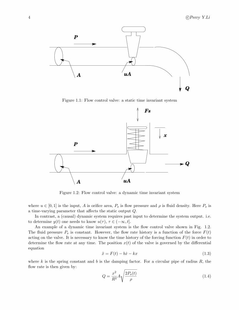
A static time invariant system is one with y(t) = f(u(t)) for all t. To determine the output ofa static system at any time t, the input value only at t is needed. Again, a light switch is a statictime invariant system. A static time-varying system is one with time-varying parameters such asexternal disturbance signals. An example is a flow control valve (Fig.1.1), whose output flow rateQ is given as

Q = uA

�2Ps(t)

ρ(1.2)

3

4 c�Perry Y.Li

A uA

Q

P

Figure 1.1: Flow control valve: a static time invariant system

A uA

Q

Fs

x

P

Figure 1.2: Flow control valve: a dynamic time invariant system

where u ∈ [0, 1] is the input, A is orifice area, Ps is flow pressure and ρ is fluid density. Here Ps isa time-varying parameter that affects the static output Q.

In contrast, a (causal) dynamic system requires past input to determine the system output. i.e.to determine y(t) one needs to know u(τ), τ ∈ (−∞, t].

An example of a dynamic time invariant system is the flow control valve shown in Fig. 1.2.The fluid pressure Ps is constant. However, the flow rate history is a function of the force F (t)acting on the valve. It is necessary to know the time history of the forcing function F (t) in order todetermine the flow rate at any time. The position x(t) of the valve is governed by the differentialequation

x = F (t)− bx− kx (1.3)

where k is the spring constant and b is the damping factor. For a circular pipe of radius R, theflow rate is then given by:

Q =x2

R2A

�2Ps(t)

ρ(1.4)

University of Minnesota ME 8281: Advanced Control Systems Design, 2001-2012 5

Earth

Orbiting pendulum

Figure 1.3: Example of a dynamic time varying system

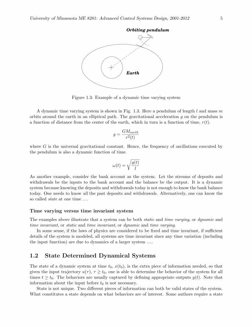
A dynamic time varying system is shown in Fig. 1.3. Here a pendulum of length l and mass morbits around the earth in an elliptical path. The gravitational acceleration g on the pendulum isa function of distance from the center of the earth, which in turn is a function of time, r(t).

g =GMearth

r2(t)

where G is the universal gravitational constant. Hence, the frequency of oscillations executed bythe pendulum is also a dynamic function of time.

ω(t) =

�g(t)

l

As another example, consider the bank account as the system. Let the streams of deposits andwithdrawals be the inputs to the bank account and the balance be the output. It is a dynamicsystem because knowing the deposits and withdrawals today is not enough to know the bank balancetoday. One needs to know all the past deposits and withdrawals. Alternatively, one can know theso called state at one time . . .

Time varying versus time invariant system

The examples above illustrate that a system can be both static and time varying, or dynamic andtime invariant, or static and time invariant, or dynamic and time varying.

In some sense, if the laws of physics are considered to be fixed and time invariant, if sufficientdetails of the system is modeled, all systems are time invariant since any time variation (includingthe input function) are due to dynamics of a larger system .....

1.2 State Determined Dynamical Systems

The state of a dynamic system at time t0, x(t0), is the extra piece of information needed, so thatgiven the input trajectory u(τ), τ ≥ t0, one is able to determine the behavior of the system for alltimes t ≥ t0. The behaviors are usually captured by defining appropriate outputs y(t). Note thatinformation about the input before t0 is not necessary.

State is not unique. Two different pieces of information can both be valid states of the system.What constitutes a state depends on what behaviors are of interest. Some authors require a state

6 c�Perry Y.Li

to be a minimal piece of information. In these notes, we do not require this to be so.

Example: Consider a car with input u(t) being its acceleration. Let y(t) be the position of the car.

1. If the behavior of interest is just the speed of the car, then x(t) = y(t) can be used as the state.It is qualified to be a state because given u(τ), τ ∈ [t0, t], the speed at t is obtained by:

v(t) = y(t) = x(t0) +

�t

t0

u(τ)dτ.

2. If the behavior of interest is the position of the car, then xa(t) =

�y(t)y(t)

�∈ �2 can be used as

the state.

3. An alternate state might be xb(t) =

�y(t) + 2y(t)

y(t)

�. Obviously, since we can determine the

old state vector xa(t) from this alternate one xb(t), and vice versa, both are valid state vectors.This illustrates the point that state vectors are not unique.

Remark 1.2.1 1. If y(t) is defined to be the behavior of interest, then by taking t = t0, thedefinition of a state determined system implies that one can determine y(t) from the statex(t) and input u(t), at time t. i.e. there is a static output function h(·, ·, ·) so that the outputy(t) is given by:

y(t) = h(x(t), u(t), t)

h : (x, u, t) �→ y(t) is called the output readout map.

2. The usual representation of continuous time dynamical system is given by the form:

x = f(x, u, t)

y = h(x, u, t)

and for discrete time system,

x(k + 1) = f(x(k), u(k), k)

y(k) = h(x(k), u(k), k)

3. Notice that a state determined dynamic system defines, for every pair of initial and finaltimes, t0 and t1, a mapping (or transformation) of the initial state x(t0) = x0 and inputtrajectory u(τ), τ ∈ [t0, t1] to the state at a time t1, x(t1). In these notes, we shall use thenotation: s(t1, t0, x0, u(·)) to denote this state transition mapping 1 . i.e.

x(t1) = s(t1, t0, x0, u(·))

if the initial state at time t0 is x0, and the input trajectory is given by u(·).

1In class (Spring 2008), we might have used the notation s(x0, u(·), t0, t1). As long as you are consistent, either

way is okay. Please be careful.


0.5

off

on

light bulb

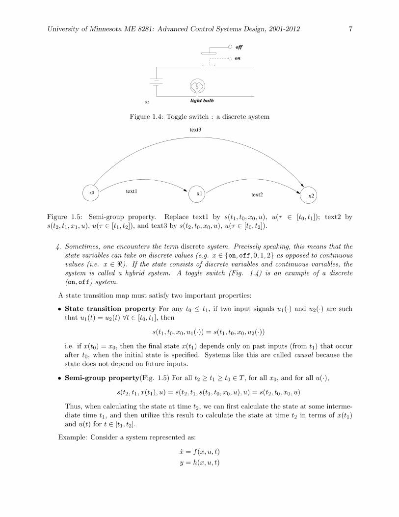
Figure 1.4: Toggle switch : a discrete system

x0 x1 x2text1 text2

text3

Figure 1.5: Semi-group property. Replace text1 by s(t1, t0, x0, u), u(τ ∈ [t0, t1]); text2 bys(t2, t1, x1, u), u(τ ∈ [t1, t2]), and text3 by s(t2, t0, x0, u), u(τ ∈ [t0, t2]).

4. Sometimes, one encounters the term discrete system. Precisely speaking, this means that thestate variables can take on discrete values (e.g. x ∈ {on, off, 0, 1, 2} as opposed to continuousvalues (i.e. x ∈ �). If the state consists of discrete variables and continuous variables, thesystem is called a hybrid system. A toggle switch (Fig. 1.4) is an example of a discrete(on, off) system.

A state transition map must satisfy two important properties:

• State transition property For any t0 ≤ t1, if two input signals u1(·) and u2(·) are suchthat u1(t) = u2(t) ∀t ∈ [t0, t1], then

s(t1, t0, x0, u1(·)) = s(t1, t0, x0, u2(·))

i.e. if x(t0) = x0, then the final state x(t1) depends only on past inputs (from t1) that occurafter t0, when the initial state is specified. Systems like this are called causal because thestate does not depend on future inputs.

• Semi-group property(Fig. 1.5) For all t2 ≥ t1 ≥ t0 ∈ T , for all x0, and for all u(·),

s(t2, t1, x(t1), u) = s(t2, t1, s(t1, t0, x0, u), u) = s(t2, t0, x0, u)

Thus, when calculating the state at time t2, we can first calculate the state at some interme-diate time t1, and then utilize this result to calculate the state at time t2 in terms of x(t1)and u(t) for t ∈ [t1, t2].

Example: Consider a system represented as:

x = f(x, u, t)

y = h(x, u, t)

8 c�Perry Y.Li

with initial condition x0 and control u(τ), τ ∈ [t0, t1]. Then the state transition map is givenas:

x(t1) = s(t1, t0, x0, u(·)) = x0 +

�t1

t0

f(x(τ), u(τ), (τ))dτ (1.5)

Notice that the solution state trajectory x(·) appears on both the left and right hand sides sothat the above equation is an implicit equation [see the section on Peano-Baker formula for lineardifferential systems].

1.3 Jacobian linearization

A continuous time, physical dynamic system is typically nonlinear and is represented by:

x = f(x, u, t) (1.6)

y = h(x, u, t) (1.7)

One can find an approximate system that is linear to represent the behavior of the nonlinear systemas it deviates from some nominal trajectory.

1. Find nominal input / trajectory One needs to find the nominal input u(·), nominal statetrajectory x(t), s.t. (1.6) (and (1.7)) are satisfied. Typically, a nominal input (or output)is given, then the nominal state and the nominal output (or input) can be determined bysolving for all t,

˙x(t) = f(x(t), u(t), t), y(t) = h(x(t), u(t), t)

2. Define perturbation. Let ∆u := u− u and ∆x := x− x, ∆y := y − y.

∆x(t) = x(t)− ˙x(t)

= f(∆x(t) + x(t),∆u(t) + u(t), t)− f(x(t), u(t), t)

3. Expand RHS in Taylor’s series and truncate to 1st order term

∆x(t) = f(∆x(t) + x(t),∆u(t) + u(t), t)− f(x(t), u(t), t)

≈ f(x(t), u(t), t) +∂f

∂x(x(t), u(t), t)∆x(t) +

∂f

∂u(x(t), u(t), t)∆u(t) +H.O.T.− f(x(t), u(t), t)

=∂f

∂x(x(t), u(t), t)∆x(t) +

∂f

∂u(x(t), u(t), t)∆u(t)

= A(t)∆x(t) +B(t)∆u(t)

Similarly,

∆y(t) ≈∂h

∂x(x(t), u(t), t)∆x(t) +

∂h

∂u(x(t), u(t), t)∆u(t)

= C(t)∆x(t) +D(t)∆u(t)

Notice that if x ∈ �n, u ∈ �m, y ∈ �p, then A(t) ∈ �n×n, B(t) ∈ �n×m, C(t) ∈ �p×n andD(t) ∈ �p×m.


Be careful that to obtain the actual input, state and output, one needs to recombine with thenominals:

u(t) ≈ u(t) +∆u(t)

x(t) ≈ x(t) +∆x(t)

y(t) ≈ y(t) +∆y(t)

Remark: In the Taylor expansion step above, the approximation can be made EXACT if weapply the mean value theorem: if f : � → � is a differentiable function then there exists a pointx� ∈ [x0, x0 +∆],

f(x0 +∆) = f(x0) +df

dx

��x�·∆

i.e. there is a point in [x0, x0+∆] such that the slope there is the mean slope between x0 and x0+∆.However, exactly what x� is not known. Nevertheless, the mean value theorem provides a way ofbounding the error in the Taylor expansion.

A similar linearization procedure can be applied to a nonlinear discrete time system

x(k + 1) = f(x(k), u(k), k)

y(k) = h(x(k), u(k), k)

about the nominal input/state/output s.t. x(k + 1) = f(x(k), u(k), k), y(k) = h(x(k), u(k), k) toobtain the linear approximation,

∆x(k + 1) = A(k)∆x(k) +B(k)∆u(k)

∆y(k) = C(k)∆x(k) +D(k)∆u(k)

with

u(t) ≈ u(t) +∆u(t)

x(t) ≈ x(t) +∆x(t)

y(t) ≈ y(t) +∆y(t)

Example: Consider the pendulum shown in Fig. 1.6. The differential equation describing theangular displacement θ is nonlinear:

(Unforced) θ = −b

lθ −

g

lsin θ (1.8)

(Forced) θ = sinωt−b

lθ −

g

lsin θ (1.9)

where b = 0.5Ns/m is the damping factor, l = 1m is the pendulum length, g = 9.81m/s2 is thegravitational acceleration, θ and θ are the angular velocity and acceleration of pendulum. Thependulum is given an initial angular displacement of 20◦.The force acting on the pendulum is asinusoidal function of frequency ω.

The responses of the nonlinear system are shown in Figs. 1.7-1.8.

• Unforced pendulum: Choose state x = [θ θ]T . Following the procedure for linearization, weobtain the linear system:

x = Ax (1.10)

where

A =

�0 1

−g/l −b/l

�

10 c�Perry Y.Li

0.5

m

l θ

mg

Figure 1.6: Example for Jacobian linearization: Pendulum

5 10 15 20 25 30

!0.2

!0.1

0.1

0.2

0.3

5 10 15 20 25 30

!0.2

!0.1

0.1

0.2

0.3

Figure 1.7: (left)Nonlinear, unforced; (right)Nonlinear, forced, ω = 1 rad/s

5 10 15 20 25 30

!0.6

!0.4

!0.2

0.2

0.4

0.6

5 10 15 20 25 30

!0.2

!0.1

0.1

0.2

0.3

Figure 1.8: (left)Nonlinear, forced, ω =�

g/l rad/s (resonance); (right)Nonlinear, forced, ω =15 rad/s


0 5 10 15 20 25 30−0.3

−0.2

−0.1

0

0.1

0.2

0.3

0.4

0 5 10 15 20 25 30−0.3

−0.2

−0.1

0

0.1

0.2

0.3

0.4

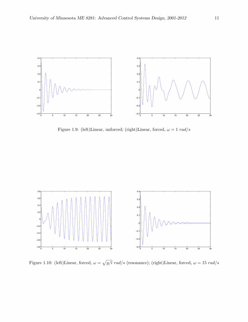
Figure 1.9: (left)Linear, unforced; (right)Linear, forced, ω = 1 rad/s

0 5 10 15 20 25 30−0.8

−0.6

−0.4

−0.2

0

0.2

0.4

0.6

0.8

0 5 10 15 20 25 30−0.3

−0.2

−0.1

0

0.1

0.2

0.3

0.4

Figure 1.10: (left)Linear, forced, ω =�g/l rad/s (resonance); (right)Linear, forced, ω = 15 rad/s

12 c�Perry Y.Li

f(x)

x

a b c d

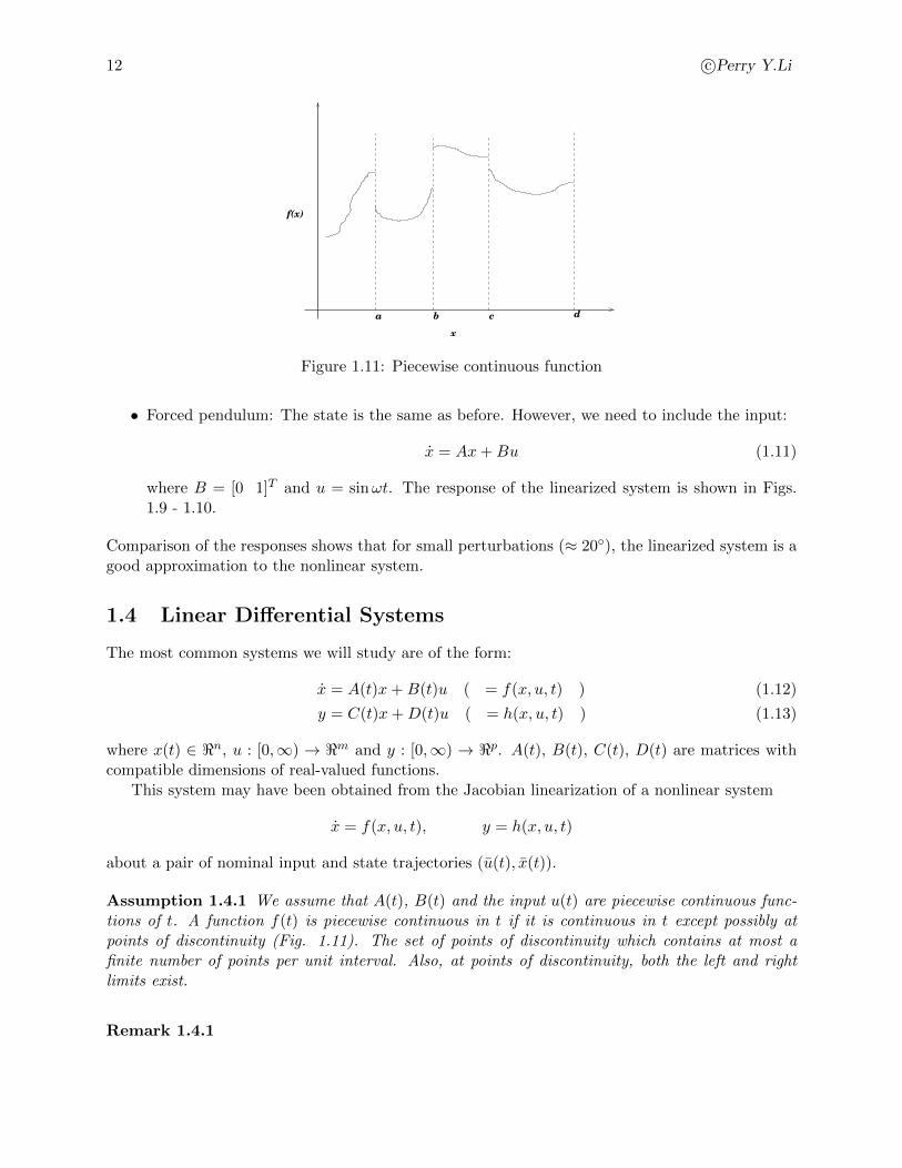
Figure 1.11: Piecewise continuous function

• Forced pendulum: The state is the same as before. However, we need to include the input:

x = Ax+Bu (1.11)

where B = [0 1]T and u = sinωt. The response of the linearized system is shown in Figs.1.9 - 1.10.

Comparison of the responses shows that for small perturbations (≈ 20◦), the linearized system is agood approximation to the nonlinear system.

1.4 Linear Differential Systems

The most common systems we will study are of the form:

x = A(t)x+B(t)u ( = f(x, u, t) ) (1.12)

y = C(t)x+D(t)u ( = h(x, u, t) ) (1.13)

where x(t) ∈ �n, u : [0,∞) → �m and y : [0,∞) → �p. A(t), B(t), C(t), D(t) are matrices withcompatible dimensions of real-valued functions.

This system may have been obtained from the Jacobian linearization of a nonlinear system

x = f(x, u, t), y = h(x, u, t)

about a pair of nominal input and state trajectories (u(t), x(t)).

Assumption 1.4.1 We assume that A(t), B(t) and the input u(t) are piecewise continuous func-tions of t. A function f(t) is piecewise continuous in t if it is continuous in t except possibly atpoints of discontinuity (Fig. 1.11). The set of points of discontinuity which contains at most afinite number of points per unit interval. Also, at points of discontinuity, both the left and rightlimits exist.

Remark 1.4.1


• Assumption 1.4.1 allows us to claim that given an initial state x(t0), and an input functionu(τ), τ ∈ [t0, t1], the solution,

x(t) = s(t, t0, x(t0), u(·)) = x(t0) +

�t

t0

[A(τ)x(τ) +B(τ)u(τ)]dτ

exists and is unique via the Fundamental Theorem of Ordinary Differential Equations (seebelow) often proved in a course on nonlinear systems.

• Uniqueness and existence of solutions of nonlinear differential equations are not generallyguaranteed. Consider the following examples.

An example in which existence is a problem:

x = 1 + x2

with x(t = 0) = 0. This system has the solution x(t) = tan t which cannot be extended beyondt ≥ π/2. This phenomenon is called finite escape.

The other issue is whether a differential equation can have more than one solution for thesame initial condition (non-uniqueness issue). e.g. for the system:

x = 3x23 , x(0) = 0.

both x(t) = 0, ∀t ≥ 0 and x(t) = t3 are both valid solutions.

Theorem 1.4.1 (Fundamental Theorem of ODE’s) Consider the following ODE

x = f(x, t) (1.14)

where x(t) ∈ �n, t ≥ 0, and f : �n ×�+ → �n.On a time interval [t0, t1], if the function f(x, t) satisfies the following:

1. For any x ∈ �n, the function t �→ f(x, t) is piecewise continuous,

2. There exists a piecewise continuous function, k(t), such that for all x1, x2 ∈ �n,

�f(x1, t)− f(x2, t)� ≤ k(t)�x1 − x2� .

Then,

1. there exists a solution to the differential equation x = f(x, t) for all t, meaning that: a) Foreach initial state xo ∈ Rn, there is a continuous function φ : R+ → Rn such that

φ(to) = x0

and

φ(t) = f(φ, t) ∀ t ∈ �

2. Moreover, the solution φ(·) is unique. [If φ1(·) and φ2(·) have the same properties above,then they must be the same.]

14 c�Perry Y.Li

Remark 1.4.2 This version of the fundamental theorem of ODE is taken from [Callier and Desoer,91]. A weaker condition (and result) is that on the interval [t0, t1], the second condition saysthat there exists a constant k[t0,t1] such that for any t ∈ [t0, t1], the function x �→ f(x, t), for allx1, x2 ∈ Rn, satisfies

�f(x1, t)− f(x2, t)� ≤ k[t0,t1]�x1 − x2� .

In this case, the solution exists and is unique on [t0, t1].

The proof of this result can be found in many books on ODE’s or dynamic systems 2 and isusually proved in details in a Nonlinear Systems Analysis class.

1.4.1 Linearity Property

The reason why the system (1.12)-(1.13) is called a linear differential system is because it satisfiesthe linearity property.

Theorem 1.4.2 For any pairs of initial and final times t0, t1 ∈ �, the state transition map

s : (t1, t0, x(t0), u(·)) �→ x(t1)

of the linear differential system (1.12)-(1.13) is a linear map of the pair of the initial state x(t0)and the input u(τ), τ ∈ [t0, t1].

In order words, for any u(·), u�(·) ∈ �m

[t0,t1], x, x� ∈ �n and α,β ∈ �,

s(t1, t0, (αx+ βx�), (αu(·) + βu�(·))) = α · s(t1, t0, x, u(·)) + β · s(t1, t0, x�, u�(·)). (1.15)

Similarly, for each pair of t0, t1, the mapping

ρ : (t1, t0, x(t0), u(·)) �→ y(t1)

from the initial state x(t0) and the input u(τ), τ ∈ [t0, t1], to the output y(t1) is also a linear map,i.e.

ρ(t1, t0, (αx+ βx�), (αu(·) + βu�(·))) = α · ρ(t1, t0, x, u(·)) + β · ρ(t1, t0, x�, u�(·)). (1.16)

Before we prove this theorem, let us point out a very useful principle for proving that two timefunctions x(t), and x�(t), t ∈ [t0, t1], are the same.

Lemma 1.4.3 Given two time signals, x(t) and x�(t). Suppose that

• x(t) and x�(t) satisfy the same differential equation,

p = f(t, p) (1.17)

• they have the same initial conditions, i.e. x(t0) = x�(t0)

• The differential equation (1.17) has unique solution on the time interval [t0, t1],

then x(t) = x�(t) for all t ∈ [t0, t1].

2e.g. Vidyasagar, Nonlinear Systems Analysis, 2nd Prentice Hall, 93, or Khalil Nonlinear Systems, McMillan, 92


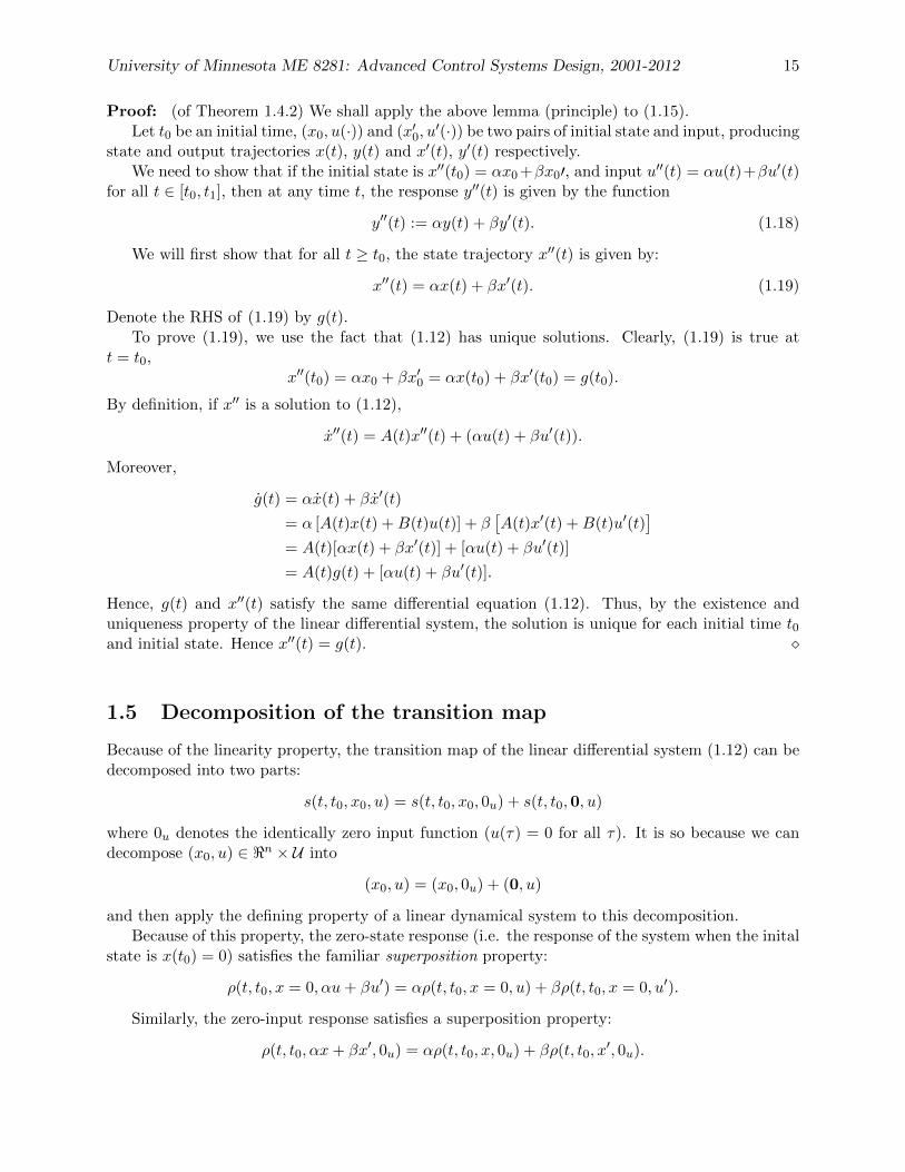
Proof: (of Theorem 1.4.2) We shall apply the above lemma (principle) to (1.15).Let t0 be an initial time, (x0, u(·)) and (x�

0, u�(·)) be two pairs of initial state and input, producing

state and output trajectories x(t), y(t) and x�(t), y�(t) respectively.We need to show that if the initial state is x��(t0) = αx0+βx0�, and input u��(t) = αu(t)+βu�(t)

for all t ∈ [t0, t1], then at any time t, the response y��(t) is given by the function

y��(t) := αy(t) + βy�(t). (1.18)

We will first show that for all t ≥ t0, the state trajectory x��(t) is given by:

x��(t) = αx(t) + βx�(t). (1.19)

Denote the RHS of (1.19) by g(t).To prove (1.19), we use the fact that (1.12) has unique solutions. Clearly, (1.19) is true at

t = t0,x��(t0) = αx0 + βx�0 = αx(t0) + βx�(t0) = g(t0).

By definition, if x�� is a solution to (1.12),

x��(t) = A(t)x��(t) + (αu(t) + βu�(t)).

Moreover,

g(t) = αx(t) + βx�(t)

= α [A(t)x(t) +B(t)u(t)] + β�A(t)x�(t) +B(t)u�(t)

�

= A(t)[αx(t) + βx�(t)] + [αu(t) + βu�(t)]

= A(t)g(t) + [αu(t) + βu�(t)].

Hence, g(t) and x��(t) satisfy the same differential equation (1.12). Thus, by the existence anduniqueness property of the linear differential system, the solution is unique for each initial time t0and initial state. Hence x��(t) = g(t). �

1.5 Decomposition of the transition map

Because of the linearity property, the transition map of the linear differential system (1.12) can bedecomposed into two parts:

s(t, t0, x0, u) = s(t, t0, x0, 0u) + s(t, t0,0, u)

where 0u denotes the identically zero input function (u(τ) = 0 for all τ). It is so because we candecompose (x0, u) ∈ �n × U into

(x0, u) = (x0, 0u) + (0, u)

and then apply the defining property of a linear dynamical system to this decomposition.Because of this property, the zero-state response (i.e. the response of the system when the inital

state is x(t0) = 0) satisfies the familiar superposition property:

ρ(t, t0, x = 0,αu+ βu�) = αρ(t, t0, x = 0, u) + βρ(t, t0, x = 0, u�).

Similarly, the zero-input response satisfies a superposition property:

ρ(t, t0,αx+ βx�, 0u) = αρ(t, t0, x, 0u) + βρ(t, t0, x�, 0u).

16 c�Perry Y.Li

1.6 Zero-input transition and the Transition Matrix

From the proof of linearity of the Linear Differential Equation, we actually showed that the statetransition function s(t, t0, x0, u) is linear with respect to (x0, u). In particular, for zero input(u = 0u), it is linear with respect to the initial state x0. We call the transition when the input isidentically 0, the zero-input transition.

It is easy to show, by choosing x0 to be columns in an identity matrix successively (i.e. invokingthe so called 1st representation theorem, namely any a finite dimensional linear function can berepresented by a matrix multiplication - Ref: Desoer and Callier, or Chen), that there exists amatrix, Φ(t, t0) ∈ �n×n so that

s(t, t0, x0, 0u) = Φ(t, t0)x0.

This matrix function is called the transition matrix. The following result gives the definingproperty a transition matrix.Theorem: Φ(t, t0) satisfies (1.12). i.e.

∂

∂tΦ(t, t0) = A(t)Φ(t, t0) (1.20)

and Φ(t0, t0) = I.Proof: Consider an arbitrary initial state x0 ∈ �n and zero input. By definition,

x(t) = Φ(t, t0)x0 = s(t, t0, x0, 0u).

Differentiating the above,

x(t) =∂

∂tΦ(t, t0)x0 = A(t)Φ(t, t0)x0.

Now pick successively n different initial conditions x0 = e1, x0 = e2, · · · , x0 = en so that{e1, · · · , en} form a basis of �n. (We can take for example, ei to be the i − th column of theidentity matrix). Thus,

∂

∂tΦ(t, t0)

�e1 e2 · · · en

�= A(t)Φ(t, t0)

�e1 e2 · · · en

�

Since�e1 e2 · · · en

�∈ �n×n is invertible, we multiply both sides by its inverse to obtain the

required answer.The initial condition Φ(t0, t0) = I because s(t0, t0, x0,00u) = Φ(t0, t0)x0 = x0 for all x0. �

With this property, one can solve for the transition matrix by integrating the differential equa-tion (1.20) with the initial condition of I at t = t0. Note that there are n2 elements to solve.

Definition 1.6.1 A n× n matrix X(t) that satisfies the system equation,

X(t) = A(t)X(t)

and X(τ) is non-singular for some τ , is called a fundamental matrix.

Remark 1.6.1 The transition matrix Φ(t, t0) is a fundamental matrix (as a function of t and t0is considered fixed). It is invertible for at least t = t0.

Proposition 1.6.1 Let X(t) ∈ �n×n be a fundamental matrix. Then, X(t) is non-singular at allt ∈ �.


Proof: Since X(t) is a fundamental matrix, X(t1) is nonsingular for some t1. Suppose that X(τ)is singular, then ∃ a non-zero vector k ∈ �n s.t. X(τ)k = 0, the zero vector in �n. Consider nowthe differential equation:

x = A(t)x, x(τ) = X(τ)k = 0 ∈ �n.

Then, x(t) = 0 for all t is the unique solution to this system with x(τ) = 0. However, the function

x�(t) = X(t)k

satisfies

x�(t) = A(t)X(t)k = A(t)x�(t),

and x�(τ) = x(τ) = 0. Thus, by the uniqueness of differential equation, x(t) = x�(t) for all t. Hencex�(t1) = 0 extracting a contradiction because X(t1) is nonsingular so x�(t1) = X(t1)k is non-zero.�

1.6.1 Properties of Transition matrices

1. (Existence and Uniqueness) Φ(t, t0) exists and is unique for each t, t0 ∈ � (t ≥ t0 is notnecessary).

2. (Group property) For all t, t1, t0 (not necessarily t0 ≤ t ≤ t1)

Φ(t, t0) = Φ(t, t1)Φ(t1, t0).

Example: For A =

�0.8147 0.12700.9058 0.9134

�, the state transition matrix Φ(t, t0) is calculated as

(to be derived later):

Φ(t, t0) = exp[A(t− t0)]

If t0 = 0, t1 = 2, t2 = 5,

Φ(t1, t0) =

�6.4051 1.544711.0169 7.6055

�

Φ(t2, t0) =

�186.38 74.814533.59 244.52

�

Φ(t2, t1) =

�18.7195 6.035043.0435 23.4097

�

Now,

Φ(t2, t1)Φ(t1, t0) =

�186.38 74.814533.59 244.52

�

= Φ(t2, t0)

3. (Non-singularity) Φ(t, t0) = [Φ(t0, t)]−1.

18 c�Perry Y.Li

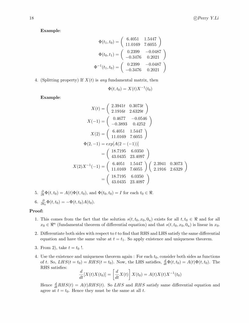
Example:

Φ(t1, t0) =

�6.4051 1.544711.0169 7.6055

�

Φ(t0, t1) =

�0.2399 −0.0487−0.3476 0.2021

�

Φ−1(t1, t0) =

�0.2399 −0.0487−0.3476 0.2021

�

4. (Splitting property) If X(t) is any fundamental matrix, then

Φ(t, t0) = X(t)X−1(t0)

Example:

X(t) =

�2.3941t 0.3073t2.1916t 2.6329t

�

X(−1) =

�0.4677 −0.0546−0.3893 0.4252

�

X(2) =

�6.4051 1.544711.0169 7.6055

�

Φ(2,−1) = exp[A(2− (−1))]

=

�18.7195 6.035043.0435 23.4097

�

X(2)X−1(−1) =

�6.4051 1.544711.0169 7.6055

��2.3941 0.30732.1916 2.6329

�

=

�18.7195 6.035043.0435 23.4097

�

5. ∂

∂tΦ(t, t0) = A(t)Φ(t, t0), and Φ(t0, t0) = I for each t0 ∈ �.

6. ∂

∂t0Φ(t, t0) = −Φ(t, t0)A(t0).

Proof:

1. This comes from the fact that the solution s(t, t0, x0, 0u) exists for all t, t0 ∈ � and for allx0 ∈ �n (fundamental theorem of differential equation) and that s(t, t0, x0, 0u) is linear in x0.

2. Differentiate both sides with respect to t to find that RHS and LHS satisfy the same differentialequation and have the same value at t = t1. So apply existence and uniqueness theorem.

3. From 2), take t = t0 !.

4. Use the existence and uniqueness theorem again : For each t0, consider both sides as functionsof t. So, LHS(t = t0) = RHS(t = t0). Now, the LHS satisfies, d

dtΦ(t, t0) = A(t)Φ(t, t0). The

RHS satisfies:d

dt[X(t)X(t0)] =

�d

dtX(t)

�X(t0) = A(t)X(t)X−1(t0)

Hence d

dtRHS(t) = A(t)RHS(t). So LHS and RHS satisfy same differential equation and

agree at t = t0. Hence they must be the same at all t.


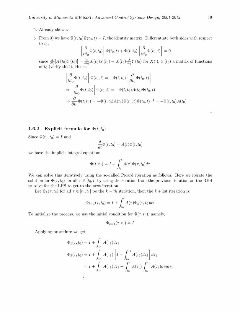
5. Already shown.

6. From 3) we have Φ(t, t0)Φ(t0, t) = I, the identity matrix. Differentiate both sides with respectto t0, �

∂

∂t0Φ(t, t0)

�Φ(t0, t) + Φ(t, t0)

�∂

∂t0Φ(t0, t)

�= 0

since d

dt0[X(t0)Y (t0)] =

d

dt0X(t0)Y (t0) +X(t0)

d

dt0Y (t0) for X(·), Y (t0) a matrix of functions

of t0 (verify this!). Hence,�

∂

∂t0Φ(t, t0)

�Φ(t0, t) = −Φ(t, t0)

�∂

∂t0Φ(t0, t)

�

⇒

�∂

∂t0Φ(t, t0)

�Φ(t0, t) = −Φ(t, t0)A(t0)Φ(t0, t)

⇒∂

∂t0Φ(t, t0) = −Φ(t, t0)A(t0)Φ(t0, t)Φ(t0, t)

−1 = −Φ(t, t0)A(t0)

�

1.6.2 Explicit formula for Φ(t, t0)

Since Φ(t0, t0) = I andd

dtΦ(t, t0) = A(t)Φ(t, t0)

we have the implicit integral equation:

Φ(t, t0) = I +

�t

t0

A(τ)Φ(τ, t0)dτ

We can solve this iteratively using the so-called Picard iteration as follows. Here we iterate thesolution for Φ(τ, t0) for all τ ∈ [t0, t] by using the solution from the previous iteration on the RHSto solve for the LHS to get to the next iteration.

Let Φk(τ, t0) for all τ ∈ [t0, t1] be the k − th iteration, then the k + 1st iteration is:

Φk+1(τ, t0) = I +

�t

t0

A(τ)Φk(τ, t0)dτ

To initialize the process, we use the initial condition for Φ(τ, t0), namely,

Φk=1(τ, t0) = I

Applying procedure we get:

Φ1(τ, t0) = I +

�τ

t0

A(τ1)dτ1

Φ2(τ, t0) = I +

�τ

t0

A(τ1)

�I +

�τ1

t0

A(τ2)dτ2

�dτ1

= I +

�τ

t0

A(τ1)dτ1 +

�τ

t0

A(τ1)

�τ1

t0

A(τ2)dτ2dτ1

...

20 c�Perry Y.Li

0 5 100

0.2

0.4

0.6

0.8

1

Time(sec)

Φ11

123456

0 5 10−2

−1

0

1

2

3

4

Time(sec)

Φ21

123456

0 5 100

0.1

0.2

0.3

0.4

Time(sec)

Φ12

123456

0 5 10−2

−1

0

1

2

3

4

Time(sec)

Φ22

123456

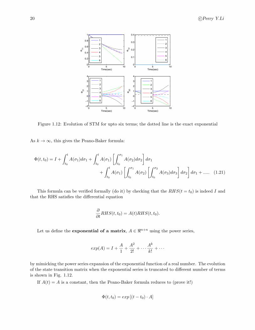
Figure 1.12: Evolution of STM for upto six terms; the dotted line is the exact exponential

As k → ∞, this gives the Peano-Baker formula:

Φ(t, t0) = I +

�t

t0

A(σ1)dσ1 +

�t

t0

A(σ1)

��σ1

t0

A(σ2)dσ2

�dσ1

+

�t

t0

A(σ1)

��σ1

t0

A(σ2)

��σ2

t0

A(σ3)dσ3

�dσ2

�dσ1 + ..... (1.21)

This formula can be verified formally (do it) by checking that the RHS(t = t0) is indeed I andthat the RHS satisfies the differential equation

∂

∂tRHS(t, t0) = A(t)RHS(t, t0).

Let us define the exponential of a matrix, A ∈ �n+n using the power series,

exp(A) = I +A

1+

A2

2!+ · · ·

Ak

k!+ · · ·

by mimicking the power series expansion of the exponential function of a real number. The evolutionof the state transition matrix when the exponential series is truncated to different number of termsis shown in Fig. 1.12.

If A(t) = A is a constant, then the Peano-Baker formula reduces to (prove it!)

Φ(t, t0) = exp [(t− t0) ·A]


For example, examining the 4th term,

�t

t0

A(σ1)

��σ1

t0

A(σ2)

��σ2

t0

A(σ3)dσ3

�dσ2

�dσ1

=A3

�t

t0

�σ1

t0

�σ2

t0

dσ3dσ2dσ1

=A3

�t

t0

�σ1

t0

(σ2 − t0)dσ2dσ1

=A3

�t

t0

(σ1 − t0)2

2dσ1 = A3

(t− t0)3

3!

A more general case is that if A(t) and�t

t0A(τ)dτ , commute for all t,

Φ(t, t0) = exp

��t

t0

A(τ)dτ

�(1.22)

An intermediate step is to show that:

1

k + 1

d

dt

��t

0

A(τ)dτ

�k+1

= A(t)

��t

t0

A(τ)dτ

�k=

��t

t0

A(τ)dτ

�kA(t).

Notice that (1.22) does not in general apply unless the matrices commute. i.e.

A(t)

��t

t0

A(τ)dτ

�k=

��t

t0

A(τ)dτ

�kA(t).

Each of the following situations will guarantee that the condition A(t) and�t

t0A(τ)dτ commute

for all t is satisfied:

1. A(t) is constant.

2. A(t) = α(t)M where α(t) is a scalar function, and M ∈ �n×n is a constant matrix;

3. A(t) =�

iαi(t)Mi where {Mi} are constant matrices that commute: MiMj = MjMi, and

αi(t) are scalar functions;

4. A(t) has a time-invariant basis of eigenvectors spanning �n.

1.6.3 Computation of Φ(t, 0) = exp(tA) for constant A

The defining computational method for Φ(t, t0) not necessarily for time varying A(t) is:

∂

∂tΦ(t, t0) = A(t)Φ(t, t0); Φ(t0, t0) = I

When A(t) = constant, there are algebraic approaches available:

Φ(t1, t0) = exp(A(t1 − t0))

:= I +A(t1 − t0)

1!+

A2(t1 − t0)2

2!+ . . .

22 c�Perry Y.Li

Matlab provides expm(A ∗ (t1 − t0)). Example :>> t0 = 2;

>> t1 = 5;>> A = [0.8147 0.1270; 0.9058 0.9134];>> expm(A ∗ (t1 − t0))ans = 18.7195 6.0350

43.0435 23.4097

Laplace transform approach

L(Φ(t, 0)) = [sI −A]−1

Proof: Since Φ(0, 0) = I, and∂

∂tΦ(t, 0) = A(t)Φ(t, 0)

take Laplace transform of the (Matrix) ODE:

sΦ(s, 0)− Φ(0, 0) = AΦ(s, 0)

where Φ(s, 0) is the Laplace transform of Φ(t, 0) when treated as function of t. This gives:

(sI −A)Φ(s, 0) = I

Example

A =

�−1 01 −2

�

(sI −A)−1 =

�s+ 1 0−1 s+ 2

�−1

=1

(s+ 1)(s+ 2)

�s+ 2 01 s+ 1

�

=

�1/(s+ 1) 0

1/(s+ 1)(s+ 2) 1/(s+ 2)

�

Taking the inverse Laplace transform (using e.g. a table) term by term,

Φ(t, 0) =

�e−t 0

e−t − e−2t e−2t

�

Similarity Transform (decoupled system) approach

Let A ∈ �n×n, if v ∈ Cn and λ ∈ C satisfy

A · v = λv

then, v is an eigenvector and λ its associated eigenvalue.If A ∈ �n×n has n distinct eigenvalues λ1, λ2, . . .λn, then A is called simple. If A ∈ �n×n has

n independent eigenvectors then A is called semi-simple (Notice that A is necessarily semi-simpleif A is simple).

Suppose A ∈ �n×n is simple, then let

T =�v1 v2 . . . vn

�; Λ = diag(λ1,λ2, . . . ,λn)


be the collection of eigenvectors, and the associated eigenvalues. Then, the so-called similaritytransform is:

A = TΛT−1 (1.23)

Remark

• A sufficient condition for A being semi-simple is if A has n distinct eigenvalues (i.e. it issimple);

• When A is not semi-simple, a similar decomposition as (1.23) is available except that Λ will bein Jordan form (has 1’s in the super diagonals) and T consists of eigenvectors and generalizedeigenvectors). This topic is covered in most Linear Systems or linear algebra textbook

Now

exp(At) := I +At

1!+

A2t2

2!+ . . .

Notice that Ak = TΛkT−1, thus,

exp(tA) = T

�I +

Λt

1!+

Λ2t2

2!+ . . .

�T−1 = Texp(Λt)T−1

The above formula is valid even if A is not semi-simple. In the semi-simple case,

Λk = diag�λk

1,λk

2, . . . ,λk

n

�

so that

exp(Λt) = diag [exp(λ1t), exp(λ2t), . . . , exp(λnt)]

If we write T−1 =

wT

1

wT

2

...wTn

where wT

iis the i-th row of T−1, then,

exp(tA) = Texp(Λt)T−1 =n�

i=1

exp(λit)viwT

i .

This is the dyadic expansion of exp(tA). Can you show that wT

iA = λiwT

i? This means that wi

are the left eigenvectors of A.The expansion shows that the system has been decomposed into a set of simple, decoupled 1st

order systems.Example

A =

�−1 01 −2

�

The eigenvalues and eigenvectors are:

λ1 = −1, v1 =

�11

�; λ2 = −2, v2 =

�01

�.

24 c�Perry Y.Li

Thus,

exp(At) =

�1 01 1

��e−t 00 e−2t

��1 0−1 1

�=

�e−t 0

e−t − e−2t e−2t

�,

same as by the Laplace transform method.

Digression: Modal decomposition The (generalized 3) eigenvectors are good basis for a coor-dinate system.

Suppose that A = TΛT−1 is the similarity transform.

Let x ∈ �n, z = T−1x, and x = Tz, Thus,

x = z1v1 + z2v2 + . . . znvn.

where T = [v1, v2, . . . , vn] ∈ �n×n.

Hence, x is decomposed into the components in the direction of the eigenvectors with zi beingthe scaling for the i−th eigenvector.

The original linear differential equation is written as:

x = Ax+Bu

T z = TΛz +Bu

z = Λz + T−1Bu

If we denote B = T−1B, then, since Λ is diagonal,

zi = λizi + Biu

where zi is the i−th component of z and Bi is the i− th row of B.

This is a set of n decoupled first order differential equations that can be analyzed indepen-dently. Dynamics in each eigenvector direction is called a mode. If desired, z can be used tore-constitute x via x = Tz.

Example: Consider the system

x =

�2 −5−1 3

�x+

�01

�u (1.24)

3for the case the A is not semi-simple, additional “nice” vectors are needed to form a basis, they are called

generalized eigenvectors


Eigenvalues: λ1 = 0.2087, λ2 = 4.7913. Eigenvectors: v1 =

�−0.9414−0.3373

�, v2 =

�0.8732−0.4874

�.

T = (v1 v2) =

�−0.9414 0.8732−0.3373 −0.4874

�

T−1 =

�−0.6470 −1.15900.4477 −1.2496

�

Λ =

�λ1 00 λ2

�

A = TΛT−1

z = T−1x

B = T−1B

=

�−1.1590−1.2496

�

z = Λz + Bu

z1 = (0.2087)z1 + (−1.1590)u

z2 = (4.7913)z2 + (−1.2496)u

Thus, the system equations obtained after modal decomposition are completely decoupled.

1.7 Zero-State transition and response

Recall that for a linear differential system,

x(t) = A(t)x(t) +B(t)u(t) x(t) ∈ �n, u(t) ∈ �

m

the state transition map can be decomposed into the zero-input response and the zero-state re-sponse:

s(t, t0, x0, u) = Φ(t, t0)x0 + s(t, t0, 0x, u)

Having figured out the zero-input state component, we now derive the zero-state response.

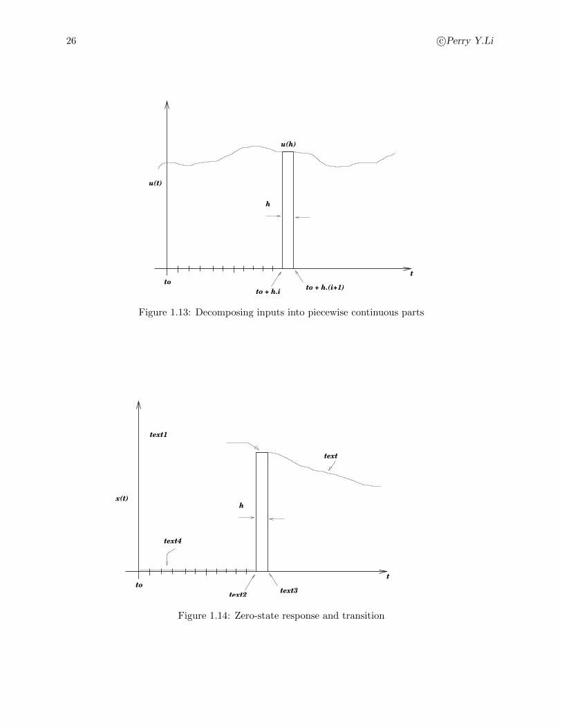
1.7.1 Heuristic guess

We first decompose the inputs into piecewise continuous parts {ui : � → �m} fori = · · · ,−2,−1, 1, 0, 1, · · · ,

ui(t) =

�u(t0 + h · i) t0 + h · i ≤ t < t0 + h · (i+ 1)

0 otherwise

where h > 0 is a small positive number (Fig. 1.13). Intuitively we can see that as h → 0,

u(t) =∞�

i=−∞ui(t) as h → 0.

Let u(t) =�∞

i=−∞ ui(t). By linearity of the transition map,

s(t, t0, 0, u) =�

i

s(t, t0, 0, ui).

Now we figure out s(t, t0, 0, ui). Refer Fig. 1.14.

26 c�Perry Y.Li

h

to

to + h.ito + h.(i+1)

t

u(t)

u(h)

Figure 1.13: Decomposing inputs into piecewise continuous parts

h

to

t

x(t)

text

text1

text2text3

text4

Figure 1.14: Zero-state response and transition


• Step 1: t0 ≤ t < t0 + h · i.

Since u(τ) = 0, τ ∈ [t0, t0 + h · i) and x(t0) = 0,

x(t) = 0 for t0 ≤ t < t0 + h · i

• Step 2: t ∈ [t0 + h · i, t0 + h(i+ 1)).

Input is active:

x(t) ≈x(t0 + h · i) + [A(t0 + h · i) +B(t0 + h · i)u(t0 + h · i)] ·∆T

= [B(t0 + h · i)u(t0 + h · i)] ·∆T

where ∆T = t− t0 + h · i.

• Step 3: t ≥ t0 + h · (i+ 1).

Input is no longer active, ui(t) = 0. So the state is again given by the zero-input transitionmap:

Φ (t, t0 + h · (i+ 1))B(t0 + i · h)u(t0 + h · i)� �� ≈x(t0+(i+1)·h)

Since Φ(t, t0) is continuous, if we make the approximation

Φ(t, t0 + (h+ 1)i) ≈ Φ(t, t0 + h · i)

we only introduce second order error in h. Hence,

s(t, t0, x0, ui) ≈ Φ(t, t0 + h · i)B(t0 + h · i)u(t0 + h · i).

The total zero-state state transition due to the input u(·) is therefore given by:

s(t, t0, 0, u) ≈

(t−t0)/h�

i=0

Φ (t, t0 + h · i)B(t0 + i · h)u(t0 + h · i)

As h → 0, the sum becomes an integral so that:

s(t, t0, 0, u) =

�t

t0

Φ(t, τ)B(τ)u(τ)dτ. (1.25)

In this heuristic derivation, we can see that Φ(t, τ)B(τ)u(τ) is the contribution to the state x(t)due to the input u(τ) for τ < t.

1.7.2 Formal Proof of zero-state transition map

We will show that for all t, t0 ∈ �+,

(x(t) = s(t, t0, 0x, u)) =

�t

t0

Φ(t, τ)B(τ)u(τ)dτ. (1.26)

Clearly (1.26) is correct for t = t0. We will now show that the LHS of (1.26), i.e. x(t) and the RHSof (1.26), which we will denote by z(t) satisfy the same differential equation.

28 c�Perry Y.Li

toto

t t

t tτ τ

σσ

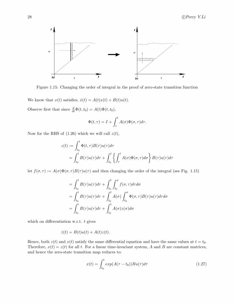
Figure 1.15: Changing the order of integral in the proof of zero-state transition function

We know that x(t) satisfies, x(t) = A(t)x(t) +B(t)u(t).

Observe first that since d

dtΦ(t, t0) = A(t)Φ(t, t0),

Φ(t, τ) = I +

�t

τ

A(σ)Φ(σ, τ)dτ.

Now for the RHS of (1.26) which we will call z(t),

z(t) :=

�t

t0

Φ(t, τ)B(τ)u(τ)dτ

=

�t

t0

B(τ)u(τ)dτ +

�t

t0

��t

τ

A(σ)Φ(σ, τ)dσ

�B(τ)u(τ)dτ

let f(σ, τ) := A(σ)Φ(σ, τ)B(τ)u(τ) and then changing the order of the integral (see Fig. 1.15)

=

�t

t0

B(τ)u(τ)dτ +

�t

t0

�σ

t0

f(σ, τ)dτdσ

=

�t

t0

B(τ)u(τ)dτ +

�t

t0

A(σ)

�σ

t0

Φ(σ, τ)B(τ)u(τ)dτdσ

=

�t

t0

B(τ)u(τ)dτ +

�t

t0

A(σ)z(σ)dσ

which on differentiation w.r.t. t gives

z(t) = B(t)u(t) +A(t)z(t).

Hence, both z(t) and x(t) satisfy the same differential equation and have the same values at t = t0.Therefore, x(t) = z(t) for all t. For a linear time-invariant system, A and B are constant matrices,and hence the zero-state transition map reduces to:

x(t) =

�t

t0

exp(A(τ − t0))Bu(τ)dτ (1.27)


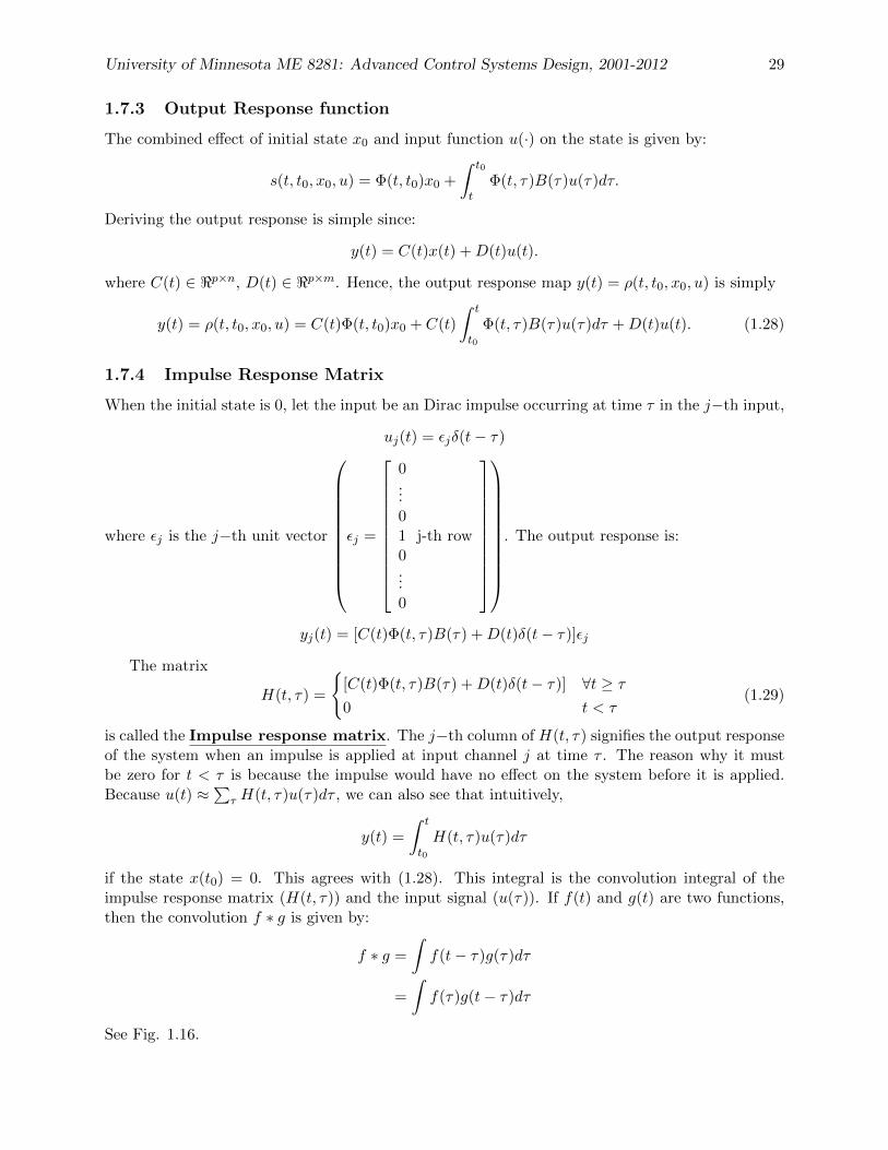
1.7.3 Output Response function

The combined effect of initial state x0 and input function u(·) on the state is given by:

s(t, t0, x0, u) = Φ(t, t0)x0 +

�t0

t

Φ(t, τ)B(τ)u(τ)dτ.

Deriving the output response is simple since:

y(t) = C(t)x(t) +D(t)u(t).

where C(t) ∈ �p×n, D(t) ∈ �p×m. Hence, the output response map y(t) = ρ(t, t0, x0, u) is simply

y(t) = ρ(t, t0, x0, u) = C(t)Φ(t, t0)x0 + C(t)

�t

t0

Φ(t, τ)B(τ)u(τ)dτ +D(t)u(t). (1.28)

1.7.4 Impulse Response Matrix

When the initial state is 0, let the input be an Dirac impulse occurring at time τ in the j−th input,

uj(t) = �jδ(t− τ)

where �j is the j−th unit vector

�j =

0...01 j-th row0...0

. The output response is:

yj(t) = [C(t)Φ(t, τ)B(τ) +D(t)δ(t− τ)]�j

The matrix

H(t, τ) =

�[C(t)Φ(t, τ)B(τ) +D(t)δ(t− τ)] ∀t ≥ τ

0 t < τ(1.29)

is called the Impulse response matrix. The j−th column of H(t, τ) signifies the output responseof the system when an impulse is applied at input channel j at time τ . The reason why it mustbe zero for t < τ is because the impulse would have no effect on the system before it is applied.Because u(t) ≈

�τH(t, τ)u(τ)dτ , we can also see that intuitively,

y(t) =

�t

t0

H(t, τ)u(τ)dτ

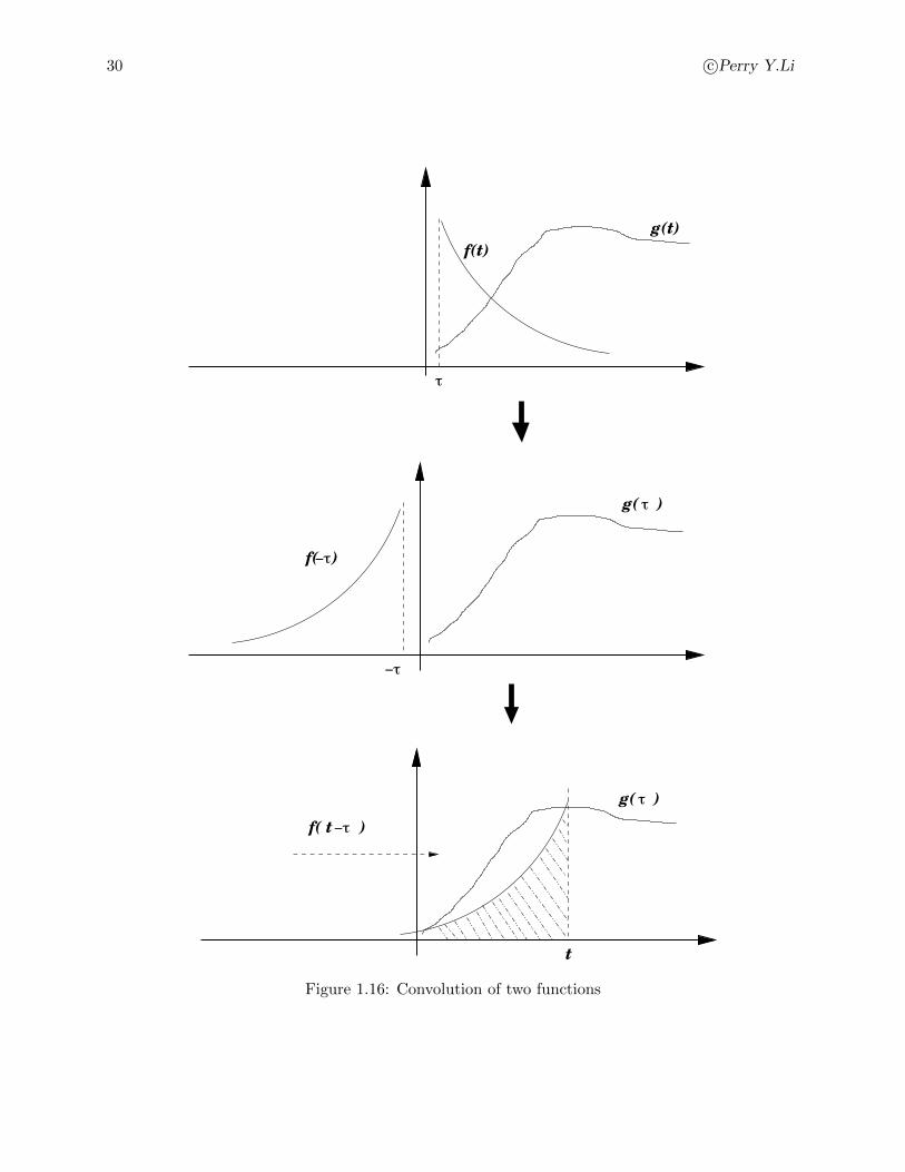
if the state x(t0) = 0. This agrees with (1.28). This integral is the convolution integral of theimpulse response matrix (H(t, τ)) and the input signal (u(τ)). If f(t) and g(t) are two functions,then the convolution f ∗ g is given by:

f ∗ g =

�f(t− τ)g(τ)dτ

=

�f(τ)g(t− τ)dτ

See Fig. 1.16.

30 c�Perry Y.Li

τ

g(t)

f(t)

−τ

f( )−τ

g( )τ

g( )τ

f( t )−τ

t

Figure 1.16: Convolution of two functions


1.8 Linear discrete time system response

Discrete time systems are described by difference equation. For any (possibly nonlinear) differenceequation:

x(k + 1) = f(k, x(k), u(k))

with initial condition x(k0), the solution x(k ≥ k0) exists and is unique as long as f(k, x(k), u(k))is a properly defined function (i.e. f(k, x, u) is well defined for given k, x, u.) This can be shownby just recursively applying the difference equation forward in time. The existence of the solutionbackwards in time is not guaranteed, however.

The linear discrete time system is given by the difference equation:

x(k + 1) = A(k)x(k) +B(k)u(k);

with initial condition given by x(k0) = x0.Many properties of linear discrete time systems are similar to the linear differential (continuous

time) systems. We now study some of these, and point out some differences.Let the transition map be given by s(k1, k0, x0, u(·)) where

x(k1) = s(k1, k0, x0, u(·)).

Linearity: For any α,β ∈ R, and for any two initial states xa, xb and two input signals ua(·)and ub(·),

s(k1, k0,αxa + βxb,αua(·) + βub(·)) = αs(k1, k0, xa, ua(·)) + βs(k1, k0, xb, ub(·))

As corollaries, we have:

1. Decomposition into zero-input response and zero-state response:

s(k1, k0, x0, u(·)) = s(k1, k0, x0, 0u)� �� zero-input

+ s(k1, k0, 0x, u(·))� �� zero-initial-state

2. Zero input response can be expressed in terms of a transition matrix,

x(k) := s(k1, k0, x0, 0u) = Φ(k, k0)x0

1.8.1 Φ(k, k0) properties

The discrete time transition function can be explicitly written as:

Φ(k, k0) = Πk−1

k�=k0A(k�)

The discrete time transition matrix has many similar properties as the continuous one, particularlyin the case of A(k) is invertible for all k. The main difference results from the possibility that A(k)may not be invertible.

1. Existence and uniqueness: Φ(k1, k0) exists and is unique for all k1 ≥ k0. If k1 < k0, thenΦ(k1, k0) exists and is unique if and only if A(k) is invertible for all k0 > k ≥ k1.

2. Existence of inverse: If k1 ≥ k0, Φ(k1, k0)−1 exists and is given by

Φ(k1, k0)−1 = A(k0)

−1A(k0 + 1)−1· · ·A(k1 − 1)−1

if and only if A(k) is invertible for all k1 > k ≥ k0.

32 c�Perry Y.Li

3. Semi-group property:Φ(k2, k0) = Φ(k2, k1)Φ(k1, k0)

for k2 ≥ k1 ≥ k0 only, unless A(k) is invertible.

4. Matrix difference equations:

Φ(k + 1, k0) = A(k)Φ(k, k0)

Φ(k1, k − 1) = Φ(k1, k)A(k − 1)

Can you formulate a property for discrete time transition matrices similar to the splitting propertyfor continuous time case?

1.8.2 Zero-initial state response

The zero-initial initial state response can be obtained easily

x(k) = A(k − 1)x(k − 1) +B(k − 1)u(k − 1)

= A(k − 1)A(k − 2)x(k − 2) +A(k − 1)B(k − 2)u(k − 2) +B(k − 1)u(k − 1)

...

= A(k − 1)A(k − 2) . . . A(k0)x(k0) +k−1�

i=k0

Πk−1

j=i+1A(j)B(i)u(i)

Thus, since x(k0) = 0 for the the zero-initial state response:

s(k, k0, 0x, u) =k−1�

i=k0

Πk−1

j=i+1A(j)B(i)u(i)

=k−1�

i=k0

Φ(k, i+ 1)B(i)u(i)

1.8.3 Discretization of continuous time system

Consider a continuous time LTI system:

x = Ax x(t0) = x0 (1.30)

The state xD(k) of the equivalent discretized system is

xD(k) = x(kT )

where T is the sampling time.

xD(k + 1) = Φ((k + 1)T, kT )xD(k)

= exp(TA)xD(k)

xD(k + 2) = exp(TA)xD(k + 1)

= exp(TA)2xD(k)


Therefore, for the interval [k0, k],

xD(k) = exp(TA)k−k0xD(k0) (1.31)

Hence, the discrete-time state transition matrix is given as:

ΦD(k, k0) = exp(TA)k−k0 (1.32)

= Φ(kT, k0T ) (1.33)

34 c�Perry Y.Li

linear dynamical systems - university of minnesota dynamical systems 1.1 system classiﬁcations and...

Documents