linear differential equations with constant coefficients
TRANSCRIPT
Linear Differential Equations With ConstantCoefficients
Alan H. SteinUniversity of Connecticut
Alan H. SteinUniversity of Connecticut Linear Differential Equations With Constant Coefficients
Linear Equations With Constant Coefficients
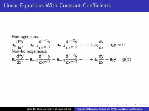
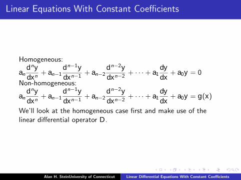
Homogeneous:
andny
dxn+ an−1
dn−1y
dxn−1+ an−2
dn−2y
dxn−2+ · · · + a1
dy
dx+ a0y = 0
Non-homogeneous:
andny
dxn+ an−1
dn−1y
dxn−1+ an−2
dn−2y
dxn−2+ · · · + a1
dy
dx+ a0y = g(x)
We’ll look at the homogeneous case first and make use of thelinear differential operator D.
Alan H. SteinUniversity of Connecticut Linear Differential Equations With Constant Coefficients
Linear Equations With Constant Coefficients
Homogeneous:
andny
dxn+ an−1
dn−1y
dxn−1+ an−2
dn−2y
dxn−2+ · · · + a1
dy
dx+ a0y = 0
Non-homogeneous:
andny
dxn+ an−1
dn−1y
dxn−1+ an−2
dn−2y
dxn−2+ · · · + a1
dy
dx+ a0y = g(x)
We’ll look at the homogeneous case first and make use of thelinear differential operator D.
Alan H. SteinUniversity of Connecticut Linear Differential Equations With Constant Coefficients
Differential Operators
Let:D denote differentiation with respect to x .
D2 denote differentiation twice.
D3 denote differentiation three times.
In general, let Dk denote differentiation k times.
The expressionf (D) = anDn + an−1Dn−1 + an−2Dn−2 + · · ·+ a1D + a0 is called adifferential operator of order n.
Alan H. SteinUniversity of Connecticut Linear Differential Equations With Constant Coefficients

Differential Operators
Given a function y with sufficient derivatives, we define
f (D)y = (anDn + an−1Dn−1 + an−2Dn−2 + · · · + a1D + a0)y
= andny
dxn+ an−1
dn−1y
dxn−1+ an−2
dn−2y
dxn−2+ · · · + a1
dy
dx+ a0y
.
This gives a convenient way of writing a homogeneous lineardifferential equation:f (D)y = 0
Alan H. SteinUniversity of Connecticut Linear Differential Equations With Constant Coefficients

Properties
We can add, subtract and multiply differential operators in theobvious way, similarly to the way we do with polynomials. Theysatisfy most of the basic properties of algebra:
I Commutative Laws
I Associative Laws
I Distributive Law
We can even factor differential operators.
Alan H. SteinUniversity of Connecticut Linear Differential Equations With Constant Coefficients

The Auxiliary Equation
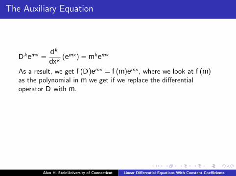
Dkemx =dk
dxk(emx) = mkemx
As a result, we get f (D)emx = f (m)emx , where we look at f (m)as the polynomial in m we get if we replace the differentialoperator D with m.
Consequence: y = emx is a solution of the differential equationf (D)y = 0 if m is a solution of the polynomial equation f (m) = 0.
We call f (m) = 0 the auxiliary equation.
Alan H. SteinUniversity of Connecticut Linear Differential Equations With Constant Coefficients
The Auxiliary Equation
Dkemx =dk
dxk(emx) = mkemx
As a result, we get f (D)emx = f (m)emx , where we look at f (m)as the polynomial in m we get if we replace the differentialoperator D with m.
Consequence: y = emx is a solution of the differential equationf (D)y = 0 if m is a solution of the polynomial equation f (m) = 0.
We call f (m) = 0 the auxiliary equation.
Alan H. SteinUniversity of Connecticut Linear Differential Equations With Constant Coefficients

The Auxiliary Equation: Distinct Roots
If the auxiliary equation f (m) = 0 has n distinct roots,m1, m2, m3, . . . mn, thenem1x , em2x , em3x , . . . , emnx are distinct solutions of the differentialequation f (D)y = 0 and the general solution isc1em1x + c2em2x + c3em3x + · · · + cnemnx .
Alan H. SteinUniversity of Connecticut Linear Differential Equations With Constant Coefficients

The Auxiliary Equation: Repeated Roots
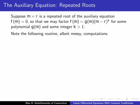
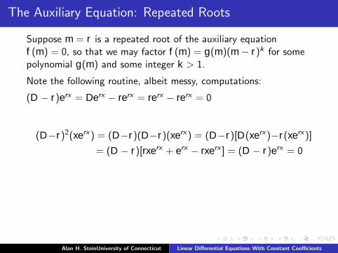
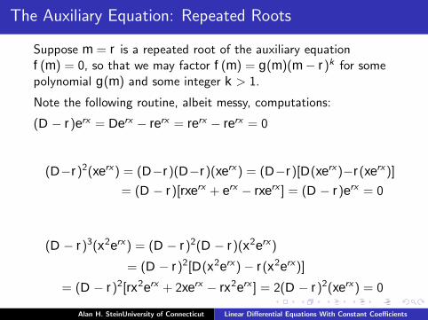
Suppose m = r is a repeated root of the auxiliary equationf (m) = 0, so that we may factor f (m) = g(m)(m − r)k for somepolynomial g(m) and some integer k > 1.
Note the following routine, albeit messy, computations:
(D − r)erx = Derx − rerx = rerx − rerx = 0
(D−r)2(xerx) = (D−r)(D−r)(xerx) = (D−r)[D(xerx)−r(xerx)]
= (D − r)[rxerx + erx − rxerx ] = (D − r)erx = 0
(D − r)3(x2erx) = (D − r)2(D − r)(x2erx)
= (D − r)2[D(x2erx) − r(x2erx)]
= (D − r)2[rx2erx + 2xerx − rx2erx ] = 2(D − r)2(xerx) = 0
Alan H. SteinUniversity of Connecticut Linear Differential Equations With Constant Coefficients
The Auxiliary Equation: Repeated Roots
Suppose m = r is a repeated root of the auxiliary equationf (m) = 0, so that we may factor f (m) = g(m)(m − r)k for somepolynomial g(m) and some integer k > 1.
Note the following routine, albeit messy, computations:
(D − r)erx = Derx − rerx = rerx − rerx = 0
(D−r)2(xerx) = (D−r)(D−r)(xerx) = (D−r)[D(xerx)−r(xerx)]
= (D − r)[rxerx + erx − rxerx ] = (D − r)erx = 0
(D − r)3(x2erx) = (D − r)2(D − r)(x2erx)
= (D − r)2[D(x2erx) − r(x2erx)]
= (D − r)2[rx2erx + 2xerx − rx2erx ] = 2(D − r)2(xerx) = 0
Alan H. SteinUniversity of Connecticut Linear Differential Equations With Constant Coefficients
The Auxiliary Equation: Repeated Roots
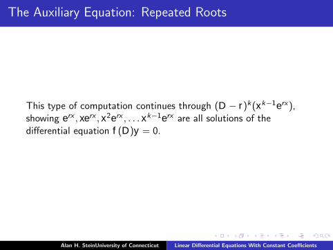
This type of computation continues through (D − r)k(xk−1erx),showing erx , xerx , x2erx , . . . xk−1erx are all solutions of thedifferential equation f (D)y = 0.
Alan H. SteinUniversity of Connecticut Linear Differential Equations With Constant Coefficients

The Auxiliary Equation: Complex Roots
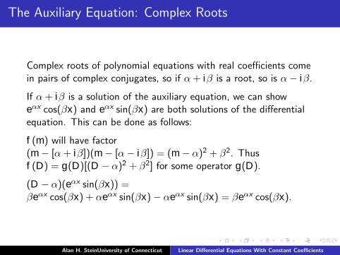
Complex roots of polynomial equations with real coefficients comein pairs of complex conjugates, so if α + iβ is a root, so is α − iβ.
If α + iβ is a solution of the auxiliary equation, we can showeαx cos(βx) and eαx sin(βx) are both solutions of the differentialequation. This can be done as follows:
f (m) will have factor(m − [α + iβ])(m − [α − iβ]) = (m − α)2 + β2. Thusf (D) = g(D)[(D − α)2 + β2] for some operator g(D).
(D − α)(eαx sin(βx)) =βeαx cos(βx) + αeαx sin(βx) − αeαx sin(βx) = βeαx cos(βx).
Alan H. SteinUniversity of Connecticut Linear Differential Equations With Constant Coefficients

The Auxiliary Equation: Complex Roots
Complex roots of polynomial equations with real coefficients comein pairs of complex conjugates, so if α + iβ is a root, so is α − iβ.
If α + iβ is a solution of the auxiliary equation, we can showeαx cos(βx) and eαx sin(βx) are both solutions of the differentialequation. This can be done as follows:
f (m) will have factor(m − [α + iβ])(m − [α − iβ]) = (m − α)2 + β2. Thusf (D) = g(D)[(D − α)2 + β2] for some operator g(D).
(D − α)(eαx sin(βx)) =βeαx cos(βx) + αeαx sin(βx) − αeαx sin(βx) = βeαx cos(βx).
Alan H. SteinUniversity of Connecticut Linear Differential Equations With Constant Coefficients

TheAuxiliaryEquation:ComplexRoots
(
D
�
�
)2
(
e�x
sin(
�
x
)))=(
D
�
�
)(
D
�
�
)(
e�x
sin(
�
x
)))=(
D
�
�
)[
�
e�x
cos(
�
x
)]=�
[�
�
e�x
sin(
�
x
)+
�
e�x
cos(
�
x
)
�
�
e�x
sin(
�
x
)=
�
�2
e�x
sin(
�
x
).
Wethusget[(
D
��
)2
+�2
](
e�x
sin(
�
x
))=
�
�2
e�x
sin(
�
x
)+
�2
e�x
sin(
�
x
)=0.
AlanH.SteinUniversityofConnecticutLinearDi�erentialEquationsWithConstantCoe�cients

The Auxiliary Equation: Complex Roots
(D − α)2(eαx sin(βx))) = (D − α)(D − α)(eαx sin(βx))) =(D − α)[βeαx cos(βx)] =β[−βeαx sin(βx)+αeαx cos(βx)−αeαx sin(βx) = −β2eαx sin(βx).
We thus get[(D−α)2+β2](eαx sin(βx)) = −β2eαx sin(βx)+β2eαx sin(βx) = 0.
Alan H. SteinUniversity of Connecticut Linear Differential Equations With Constant Coefficients
Multiple Complex Roots
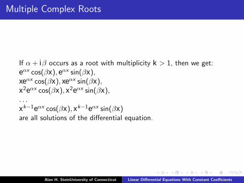
If α + iβ occurs as a root with multiplicity k > 1, then we get:eαx cos(βx), eαx sin(βx),xeαx cos(βx), xeαx sin(βx),x2eαx cos(βx), x2eαx sin(βx),. . .xk−1eαx cos(βx), xk−1eαx sin(βx)are all solutions of the differential equation.
Alan H. SteinUniversity of Connecticut Linear Differential Equations With Constant Coefficients

Nonhomogeneous Equations
Consider two distinct solutions y1, y2 of a nonhomogeneous lineardifferential equation f (D)y = g(x).
It follows thatf (D)(y1 − y2) = f (D)y1 − f (D)y2 = g(x) − g(x) = 0.
In other words, the difference between two solutions of anonhomogeneous differential equation is a solution of the relatedhomogeneous equation.
Consequence: If we find any particular solution yp of anonhomogeneous equation and yg is the general solution of therelated homogeneous differential equation, then yg + yp is thegeneral solution of the nonhomogeneous equation.
So, once we solve the related homogeneous equation, we just haveto find one solution of the nonhomogeneous equation.
Alan H. SteinUniversity of Connecticut Linear Differential Equations With Constant Coefficients

Nonhomogeneous Equations
Consider two distinct solutions y1, y2 of a nonhomogeneous lineardifferential equation f (D)y = g(x). It follows thatf (D)(y1 − y2) = f (D)y1 − f (D)y2 = g(x) − g(x) = 0.
In other words, the difference between two solutions of anonhomogeneous differential equation is a solution of the relatedhomogeneous equation.
Consequence: If we find any particular solution yp of anonhomogeneous equation and yg is the general solution of therelated homogeneous differential equation, then yg + yp is thegeneral solution of the nonhomogeneous equation.
So, once we solve the related homogeneous equation, we just haveto find one solution of the nonhomogeneous equation.
Alan H. SteinUniversity of Connecticut Linear Differential Equations With Constant Coefficients

Solving a Nonhomogeneous Equation
If g(x) involves only polynomials, exponentials, sines or cosines, orsums and products of such functions, a particular solution can befound by the Method of Undetermined Coefficients or JudiciousGuessing.
We take the individual terms of g(x) along with all theirderivatives, of all orders, ignoring constant coefficients. With theform for g(x) given, this will be a finite set. It may be very tediousto find all of them, but it is a routine, mechanical task.
Some linear combination of this collection of terms will be asolution of the differential equation. We can find which one bywriting down an arbitrary linear combination, plugging it into thedifferential equation, and then equating like coefficients on the twosides.
This is reminiscent of the method of partial fractions used tocalculate integrals involving rational functions.
Alan H. SteinUniversity of Connecticut Linear Differential Equations With Constant Coefficients
Solving a Nonhomogeneous Equation
If g(x) involves only polynomials, exponentials, sines or cosines, orsums and products of such functions, a particular solution can befound by the Method of Undetermined Coefficients or JudiciousGuessing.
We take the individual terms of g(x) along with all theirderivatives, of all orders, ignoring constant coefficients.
With theform for g(x) given, this will be a finite set. It may be very tediousto find all of them, but it is a routine, mechanical task.
Some linear combination of this collection of terms will be asolution of the differential equation. We can find which one bywriting down an arbitrary linear combination, plugging it into thedifferential equation, and then equating like coefficients on the twosides.
This is reminiscent of the method of partial fractions used tocalculate integrals involving rational functions.
Alan H. SteinUniversity of Connecticut Linear Differential Equations With Constant Coefficients

Solving a Nonhomogeneous Equation
If g(x) involves only polynomials, exponentials, sines or cosines, orsums and products of such functions, a particular solution can befound by the Method of Undetermined Coefficients or JudiciousGuessing.
We take the individual terms of g(x) along with all theirderivatives, of all orders, ignoring constant coefficients. With theform for g(x) given, this will be a finite set. It may be very tediousto find all of them, but it is a routine, mechanical task.
Some linear combination of this collection of terms will be asolution of the differential equation. We can find which one bywriting down an arbitrary linear combination, plugging it into thedifferential equation, and then equating like coefficients on the twosides.
This is reminiscent of the method of partial fractions used tocalculate integrals involving rational functions.
Alan H. SteinUniversity of Connecticut Linear Differential Equations With Constant Coefficients
Solving a Nonhomogeneous Equation
If g(x) involves only polynomials, exponentials, sines or cosines, orsums and products of such functions, a particular solution can befound by the Method of Undetermined Coefficients or JudiciousGuessing.
We take the individual terms of g(x) along with all theirderivatives, of all orders, ignoring constant coefficients. With theform for g(x) given, this will be a finite set. It may be very tediousto find all of them, but it is a routine, mechanical task.
Some linear combination of this collection of terms will be asolution of the differential equation. We can find which one bywriting down an arbitrary linear combination, plugging it into thedifferential equation, and then equating like coefficients on the twosides.
This is reminiscent of the method of partial fractions used tocalculate integrals involving rational functions.
Alan H. SteinUniversity of Connecticut Linear Differential Equations With Constant Coefficients