Limited Risk Sharing and International Equity Returns

Shaojun A. Zhang∗

Oct 2014

Abstract

I study international consumption risk sharing with limited stock market participation in eachcountry. I present new evidence, employing micro-level household consumption data in the U.S.and U.K., showing that stockholders’ consumption growth correlation is considerably higher thanthat of the aggregate consumption growth. Empirically, for stock markets that are integrated withthe U.S. market (such as European markets), U.S. stockholders long-run consumption growth canexplain its equity cross-section, but not that of segmented markets. I construct an incompletemarket model that features limited risk sharing within each country due to limited stock marketparticipation. Besides matching the salient features of asset prices (high and volatile equity pre-mium, low and smooth risk free rate), the model quantitatively rationalizes the empirical evidenceabove, as well as the low aggregate consumption growth correlation and high asset return correla-tion. The model suggests that financial integration significantly reduces the consumption volatilityof the stockholders and the amount of aggregate risks borne by them, hence improves their welfare.However, the benefits are almost all captured by the stockholders.

Keywords: comovement, consumption risk sharing, equity premium puzzle, financial integra-tion, international diversification, international equity markets, limited stock market participationJEL classification: F30, F41, F44, F62, F65, G11, G12, G15

∗School of Economics and Finance, The Univeristy of Hong Kong. Email: aszhang@hku.hk. I thank

my thesis committee Stijn van Nieuwerburgh, Matteo Maggiori, Thomas Mertens, and Robert Whitelaw for

many valuable discussions. I would also like to thank Viral Acharya, David Backus, Aurel Hizmo, Anthony

Lynch, Thomas Philippon, and Jianfeng Yu, as well as seminar participants at Georgetown McDonoungh,

HKU SEF, Hofstra, UMN Carlson, NYU Stern, OSU Fisher, PSU Smeal, Purdue Krannert, Tsinghua

PBCSF. All errors are my own.

Stock markets around the world exhibit high correlations in returns relative to the cor-

relations in aggregate economic fundamentals. In the post Bretton Woods period, the U.S.

quarterly equity return has an average correlation of 0.6 with that of Australia, Canada,

France, Germany, Italy and the United Kingdom, as shown in Table 1. The same correlation

of their financial income growth (defined as corporate profit minus investment) is 0.02, and

that of non-durable consumption growth is 0.09.

This discrepancy between the financial and fundamental correlation increases along the

dimension of financial integration, in both the time-series and the cross-section. By 2011,

U.S. investors held as much as 24% of the market capitalization of the U.K. stock market,

which was only 13% in 1997. 1 From 1973 to 1996, the quarterly return correlation between

U.S. and U.K. equity indices is 0.64, rising to 0.88 from 1997 to 2013, while the correlation

of their economic fundamentals exhibits no such increase.2

In the cross-section, the fraction of the foreign market capitalization held by U.S. investors

in 1997 is strongly positively correlated with the subsequent return correlation between the

foreign and U.S. stock market from 1998 to 2013, and explains 22% of the variation (see

Figure 1). The consumption growth correlation remains low across.

Therefore, the asset market and the macro quantity-based views give very different an-

swers to the following questions: 1) Is the current consumption risk sharing between finan-

cially integrated countries good or bad? 2) What is the potential gain (or the historical gain)

from the global financial integration?

The typical approach for making the connection is to consider alternative preferences or

shocks regarding the representative agent in each country. What is largely ignored, often

for modeling convenience or due to data restriction, is the limited risk sharing within a

country. In particular, in the U.S., only about 50% of individuals invest in the stock market,

1I use 1997 as the dividing point, since 1997 is the earliest date when the bilateral investment data areavailable.

2The literature has not reached a consensus over the magnitude and direction of these correlation changes.For example, Heathcote and Perri (2004) documents that the correlation of GDP and consumption betweenU.S. and the rest or the world decreased from 0.76 and 0.51 pre-1986 to 0.26 and 0.13 post-1986. However,Kose, Otrok, and Prasad (2010) show that during the period of financial globalization (1985-2008), there is asmall convergence of business cycle fluctuations among developed countries, but also a concomitant declinein the relative importance of the global factor.

1

either directly or indirectly (e.g., via investment vehicles for retirement or non-retirement

accounts). The participation rate tends to be lower in Europe (Grinblatt, Keloharju, and

Linnainmaa, 2011).

The limited stock market participation leads to significantly different consumption risk

sharing patterns within a country. A novel dataset of U.S. and U.K. household-level con-

sumption survey reveals that from 1988 to 2007, the 12-quarter consumption growth corre-

lation between U.S. and U.K stockholders is as high as 0.5, compared to 0.2 for the non-

stockholders. The correlation of the aggregate is only 0.3.

Since the stockholders are the marginal agents in pricing the assets, the evidence can

potentially reconcile the asset market view and the macro quantity view. I provide an

incomplete market model to quantitatively evaluate the conjecture. I adopt the consumption

risk sharing framework in the tradition of Obstfeld (1994a, b), but model the limited risk

sharing both within and between countries.

The imperfect risk sharing within a country arises due to the limited stock market par-

ticipation. There are two types of agents in each country: non-stockholders only trade in a

global bond market, whereas stockholders have access to the two stock markets as well as the

bond market. The risk sharing between countries is also imperfect, due to the undiversifiable

labor income risks.

The model quantitatively explains the dichotomy between the correlation in returns and

quantities. Home stockholders aggressively diversify their income risk with the foreign stock-

holders by directly holding the foreign equity, as well as actively re-balancing their portfolio

positions. The correlation of their consumption growths is high (0.5 in both model and

data). Equity returns reflect the risk sharing between the marginal pricers of the asset, or

the stockholders, therefore, are highly correlated (0.8 in both model and data). The non-

stockholders, nevertheless, can only smooth their consumption through the bond market. It

leads to low correlation in their consumption growths and further the low correlation in the

aggregate consumption growths (0.3 in both model and data).

Noticeably, the model delivers a low and smooth risk free-rate, together with a high and

2

volatile equity risk premium, thanks to the preference heterogeneity. In the model, non-

stockholders have lower elasticity of intertemporal substitution (EIS, 0.1) than stockholders

(0.3), consistent with empirical estimates.3 To smooth away consumption fluctuations due

to the country idiosyncratic labor income risks, the non-stockholders actively borrow and

lend with each other. For the global aggregate labor income risks, the stockholders provide

insurance to the non-stockholders, because they are more willing to substitute intertempo-

rally. Hence, the global aggregate risk is concentrated on stockholders, and they require a

high equity risk premium for compensation.

The incompleteness within a country allows reassessing the welfare of financial integra-

tion, and analyzing distributive effects. When stock markets are closed to foreign investors,

all consumption smoothing can only be conducted through the bond market, and within a

country only. Since the bond is an inefficient way to achieve the purpose, the cross-country

correlation risk sharing is very limited for all agents. Equity return correlation is also low.

The stockholders have to insure the domestic non-stockholders against a large fraction of

country-specific labor income shocks. Therefore, the equity claim appears very risky to them,

and carries high risk premium.

As soon as the stock market open up to foreign investors, in other words, when financial

markets integrate, stockholders can diversify away a significant amount of country-specific

risk through the international equity market. This accompanies an increase in the con-

sumption growth correlation for the stockholders. Naturally, the return correlation between

countries dramatically rises: The common discount rate effect dominates the low cash flow

correlation. This is consistent with the the increase of return correlation between the U.K.

and U.S., as well as in the cross-section of countries as the level of financial integration

increases.

The stockholders reaps a lot of benefit from the financial integration in terms of welfare.

Now, the stockholders only need to insure the non-stockholders against the global labor

income shocks, but not the country-specific. Further, they now only bear the global, but

3See Attanasio, Banks, and Tanner (2002), Brav, Constantinides, and Geczy (2002) and Vissing-Jorgensen(2002).

3

not country-specific, financial income risk, by taking advantage of the foreign investment

opportunities. This leads to a fall in their consumption volatility. So, they not only have

need to provide less aggregate insurance, but the cost of providing the insurance is low also.

Nevertheless, the non-stockholders are excluded from this financial advance. They bear

as much income risk as in the financial segmentation scenario and their consumption is

also as volatile. Welfare calculation shows that, the financial integration favors different

asset holders and in an extreme way: The stockholders capture almost all of the welfare

improvement from the financial integration.

1 Related Literature

The limited stock market participation literature has achieved success in closed-economy

pricing. For example, Basak and Cuoco (1998), Gomes and Michaelides (2008) and Gu-

venen (2009) show that accounting for limited participation can help rationalize the high

equity risk premium. Empirically, Vissing-Jorgensen (2002), Attanasio, Banks, and Tanner

(2002), Parker and Julliard (2005) and Malloy, Moskowitz, and Vissing-Jorgensen (2009)

find evidence on the pricing ability of the stockholders consumption growth. I bring the

limited stock market participation into the international context and provide, to my knowl-

edge, the first empirical evidence on the pricing of international assets from the perspective

of domestic stockholders.

The disconnect of asset prices from economic fundamentals in international finance draws

a lot of attention, starting from Cole and Obstfeld (1991) in the endowment economy frame-

work and Backus, Kehoe, and Kydland (1992) in the production economy framework. One

strand of literature, for example Lewis (1998), Kehoe and Perri (2002) and Bai and Zhang

(2012) among others, focuses on investigating the frictions required in order to generate the

excessive low consumption correlation in data. Another strand of literature studies the risk

sharing and asset prices jointly, such as Dumas (1992), Farhi and Gabaix (2008), Verdelhan

(2010), Colacito and Croce (2011) and Pavlova and Rigobon (2007, 2012).4 Most of this line

4Amongst others see also: Stathopoulos (2012), Hassan (2013), Martin (2011), Heyerdahl-Larsen (2012),

4

of research assume complete markets5. I instead take an incomplete market view and more

importantly, deviate from the homogeneity assumption of each countrys population. Theo-

retical analysis demonstrates that the different access to stock markets, hence risk sharing

opportunities, helps connect risk sharing with asset prices. I also exploit a novel dataset

and provide new empirical evidence on the different levels of cross-country risk sharing for

different asset holders, consistent with the model.

In parallel with the theoretical work, a growing empirical literature provides evidence

on the linkage between international asset pricing and economic fundamentals, for instance,

Lustig and Verdelhan (2007) and Borri and Verdelhan (2011) for currency and sovereign

bond returns respectively.6 I add to the literature by providing evidence on the pricing of

international equity returns in consumption CAPM framework.

My research further studies the impacts of financial integration, especially the stock mar-

ket integration. The literature on its asset pricing implications focuses mainly on emerging

markets. For example, Bekaert and Harvey (1997) document in event studies that the corre-

lation between the emerging market and the world market increases after the domestic stock

market opens up. 7

I document that globally there is a tight relation between cross-country asset returns and

asset holding shares, as well as provide a theoretical framework to analyze the mechanism

and its quantitative impacts.

Obstfeld (1998) is one of the first to examine the welfare impact of financial integra-

tion. More recent work, such as Colacito and Croce (2010), Favilukis, Ludvigson, and

Van Nieuwerburgh (2010), Martin (2010) and Lewis and Liu (2012) attempts to estimate

the aggregate welfare impacts in asset pricing context. I instead highlight the distributional

perspective, i.e, who benefits more from this process.

Farhi et al. (2009).5Notable exceptions include Alvarez, Atkeson, and Kehoe (2009) which studies time-varying levels of

market segmentation, and Maggiori (2011) as well as Gabaix and Maggiori (2013) which examine the role offinancial intermediation

6See also Brunnermeier, Nagel, and Pedersen (2009), Lustig, Roussanov, and Verdelhan (2010), Lettau,Maggiori, and Weber (2013), Jurek (2014).

7There is another strand literature that studies the determinates and measurements of financial integra-tion, see Stulz (1981), Schindler (2008), Bekaert et al. (2011) and Karolyi and Stulz (2003) etc.

5

My research is also part of the recent theoretical effort to incorporate portfolio choices in

international macro finance models. The related literature includes Devereux and Sutherland

(2009, 2011) and Pavlova and Rigobon (2010, 2012) among others.8

The rest of the paper is organized as follows. In Sections 2 and 3, I describe the empirical

framework, hypotheses, and results. I construct the theoretical framework, featuring limited

participation, in Section 4. In Sections 5 and 6, I report the quantitative results and explore

the empirical implications. In Section 7, I provide concluding remarks.

2 Empirical Preliminaries

In this section, I describe the data sets adopted, calculate the correlation of U.S. and U.K.

consumption growth rates for stockholders and non-stockholders.

2.1 The Consumption Data

I start by introducing the two household-level consumption survey data.

The U.S. Consumption Data

I draw the U.S consumption data from the Consumer Expenditure Survey (CEX) data of

the U.S. for the period 1982-2012. I calculate the quarterly consumption growth rates for

stockholders and non-stockholders respectively. The CEX data over a shorter sample period

have been used in previous studies, such as Vissing-Jorgensen (2002) and Malloy, Moskowitz,

and Vissing-Jorgensen (2009) (MMV hence) among others.

The CEX data are available from 1980: Q1 to 2012: Q1. Each household in the sample

was surveyed five times, three months apart. I identify stockholders, following Vissing-

Jorgensen (2002), based on the response to the survey question indicating positive holdings

of “stocks, bonds, mutual funds and other such securities” on the last day of last month.

Households also report the change in positions from a year ago. I require households to hold

8See also Bacchetta and Van Wincoop (2010), Tille and Van Wincoop (2010) and Duzhak, Mertens, andZhang (2013).

6

a positive amount of securities a year ago. I discuss further details of the sample and data

construction in the Appendix.

Aggregation of Household Consumption Growth Rates

I calculate the non-durable consumption growth rates for each household. The quarterly

consumption growth rate for a particular group g (stockholders/non-stockholders) from t to

t+ 1 is defined as

1

Hgt

Hgt∑

h=1

(ch,gt+1 − c

h,gt

)where ch,gt is the log quarterly consumption of household h in group g at time t, and Hg

t

denotes the number of households of group g at time t.

The U.K. Consumption Data

For the U.K. consumption growth, I use the U.K. Family Expenditure Survey(FES) data

from 1988 and 2000, and the U.K. Expenditure and Food Survey (EFS) data from 2001 to

2007. The data are used by Attanasio, Banks, and Tanner (2002) and Blundell and Etheridge

(2010) among others. I again discuss the details about data in the Appendix for brevity.

Attanasio, Banks, and Tanner (2002) point out that it is important to adjust for the

increase in the stock market participation in U.K.. They report that the increase in the level

of direct share ownership in the U.K. is “precarious” during 1985 - 1987, due to a number

of measures to promote “share-owning democracy”. It starts to stabilize in 1988. Therefore,

1988 is chosen as the start point of the sample. In 2001, this dataset merged with the UK

National Food Survey to create the Expenditure and Food Survey (EFS), and I refer to

both datasets as FES is the text below. Stockholders are identified by their response to the

question “How much is invested in stocks/shares at present”.

7

Aggregation of Household Consumption Growth Rates

The FES data are repeated cross-section, rather than panel data, which forces me to assume

a representative agent within each stockholder- and non-stockholder-group, in order to de-

termine the consumption growth rate of each group. The log consumption growth rate is

calculated as

1

Hgt+s+1

Hgt+s+1∑h=1

ch,gt+1+s −1

Hgt+s

Hgt+s∑h=1

ch,gt+s

where c denotes the per capita log consumption level and Hg denotes the number of house-

holds in group g.

I calculate the per capita non-durable consumption data per period, equalized by the

OECD (Organisation for Economic Co-operation and Development) adult equalization mea-

sure. To remove seasonality in the data, I further regress the change in the log consumption

on a set of monthly dummies, and use the residual as the quarterly consumption growth

measure.

2.2 Correlation of U.S. and U.K. consumption growth rates

I calculate the correlation of consumption growth rates for U.S. and U.K. stockholders and

non-stockholders. Results are reported in Table 2. For ease of presentation, I only report

the average for U.S. and U.K., for the within-country correlation, and the cross-country

correlation between the stockholders and the non-stockholders. I recover the correlation

of aggregate consumption growth rates from the two survey data sets, which is low, as

emphasized in the literature.

The result shows that:

corr(∆cUS,stockholders,∆cUK,stockholders) > corr(∆cUS,aggregate,∆cUK,aggregate)

corr(∆cUS,stockholders,∆cUK,stockholders) > corr(∆cUS,non−stockholders,∆cUK,non−stockholders)

corr(∆ci,stockholders,∆cj,stockholders) > corr(∆ci,stockholders,∆cj,non−stockholders)

8

where i, j ∈ {U.S., U.K.}, i 6= j.

In sum, although the aggregate consumption correlation between U.S. and U.K. is low

(0.31 at 12-quarter horizon), the consumption correlation between U.S. and U.K. stockhold-

ers is much higher (0.51 at 12-quarter horizon).

3 Empirical Asset Pricing Results

Before explaining the model, I test the following key empirical predictions of the reasoning:

Home stockholders’ consumption growth a) can price both home and integrated foreign

stock markets, and can price them better than that of non-stockholders; b) but cannot price

the segmented foreign stock markets.

The tests are important for at least two reasons: First, if empirically prediction a) holds,

it could help ensure that the model about financial integration is a sensible description of the

world to begin with; second, if prediction b) holds, it provides evidence about the dispersion

in the degree of integration between countries. I briefly describe the test and present a main

result here. I refer readers to an earlier version of this paper for full tests with robustness

tests.

3.1 Empirical Framework for Asset Pricing Tests

I adopt recursive preference specification following Kreps and Porteus (1978), Epstein and

Zin (1989), and Weil (1989). I follow the formulation in Hansen, Heaton, and Li (2008), and

the empirical implementation of MMV (2009).

Stockholders have recursive preferences of the form

Vt =

[(1− β)C

1− 1σ

t + β(Et[V1−γt+1 ])

1− 1σ

1−γ

] 1

1− 1σ

(1)

Following MMV (2009), I assume that the growth rate of the log consumption ct is a

9

linear function of the state of the economy xt, which evolves according to a first-order VAR:

ct+1 − ct = µc + Ucxt + λ0wt+1 (2)

xt+1 = Gxt +Hwt+1 (3)

I focus on the special case where the EIS (for stockholders) equals one. To avoid the

potentially imprecise results from estimating conditional expectations over a relatively short

sample period, I estimate equation (??) using only the unconditional covariance term, con-

sistent with MMV (2009)’s baseline approach. This approach leads to a consistent es-

timate of γ, if the expected return is constant over time, or if cov(Et∑∞

s=0 βs(ct+1+s −

ct+s), Et

(rit+1 − r

ft+1

)) is identical across the set of test assets (i.e., all expected asset re-

turns in the same way when the consumption growth rate varies). I include a constant term

in the regression to ensure the consistent estimate of γ in this specification. 9 Therefore, the

equation simplifies to

E(rit+1 − rft+1) +

1

2V (rit+1)−

1

2V (rft+1)

≈(γ − 1)cov(∞∑s=0

βs(ct+1+s − ct+s), rit+1 − rft+1)

(4)

I use ct to denote the sample estimate of ct. The I estimate the equation via Generalized

Method of Moments (GMM), following MMV (2009). The point estimate is equivalent to

that obtained from OLS.

3.2 Hypotheses Testing

The European market is a good candidate for a market integrated with U.S.. The European

financial market is open, with few regulatory restrictions. From the U.S. point of view,

Europe shares a lot of similarities from language and institutions to culture. Absent most

physical and informational frictions, European markets are popular hosts of U.S. foreign

9MMV (2009) shows that explicitly imposing a VAR structure on the consumption growth to estimatethe covariance does not change the results, using 25 Fama-French portfolios for the U.S..

10

equity investments. In 1997, the U.S. investors hold 11.7 percent of the European market

capitalization, which increased to 17.7 percent in 2007.

Table 3 reports the results using the 25 Fama-French portfolios with European assets.

Panel A covers the estimation using U.S. stockholder consumption growth rates. The implied

risk aversion in order to price the cross section from 8Q onwards is around 10, similar to the

estimates from the 25 U.S. Fama-French portfolio. The R2 is in general lower than when

I use the 25 U.S. portfolios as test assets; however, it is still high. Taken together, the

evidence lends strong support to the pricing ability of U.S. stockholder consumption risk for

European assets.

Panel B reports the estimates using U.S. non-stockholder consumption growth rates.

The implied risk aversion estimates are unstable, and not statistically different from 0. This

variable explains virtually none of the cross-sectional variation.

There are two reasons why the U.S. non-stockholder consumption risk fails to price the

European markets. First, non-stockholders do not hold the assets to begin with, therefore,

their Euler equation does not necessarily hold with respect to these assets. In the domes-

tic asset case, the U.S. non-stockholders’ consumption growth rate has a certain amount

of pricing ability, due to the correlation of their long-run consumption growth rates with

the domestic stockholders. However, it completely fails using the European test assets.

This result implies that the correlation of consumption growth between a typical US non-

stockholder with a typical European stockholder (the natural pricer of the European assets)

is low, consistent with Table 2.

Second, the EIS of non-stockholders is estimated to be lower than reported for stock-

holders in the literature, and hence is significantly different from 1. For instance, Barsky

et al. (1997) estimate the distribution of the EIS parameter in the population and find the

average to be below 0.3, but the highest percentiles exceed unit elasticity. Vissing-Jogensen

(2002) finds that for risky asset holders the EIS estimate is greater than 0.3, while for the

remaining households, the estimates are small and insignificantly different from 0.

The level of financial integration from the U.S. investors’ perspective significantly differs

11

across countries. In 1997, the U.S. holds in 6.1 percent of the Japanese stock market. For

comparison, the median level of market fraction that U.S. investors held is 7.5% in 1997.

Similarly, for countries in the Asian (ex-Japan) portfolio (i.e., Australia, Hong Kong, New

Zealand, and Singapore), the fraction of local market capitalization is 8.4% in 1997, and it

remained at a similar level for the next decade. Although these countries have open foreign

investment policies and few restrictions, the geographic distance (Portes and Rey, 2005) may

have prevented U.S. investors from making them primary investment destinations. More-

over, as Van Nieuwerburgh and Veldkamp (2009) shows, through active learning, investors

could amplify an initial small informational advantage (toward home countries and culturally

approximate European countries), and largely avoid investing in the others (such as Asian

countries in this case). Therefore, I consider the Asia-Pacific markets as segmented from the

U.S. markets.

Tables 4 and 5 report the estimates from the regression using Japanese assets and Asia-

Pacific (ex. Japan) respectively. In sharp contrast to the previous results, the empirical

model prices the assets of segmented markets poorly. The risk aversion estimates are un-

stable, and mostly are not statistically different from 0. The R2 is close to 0 in most cases.

Therefore, U.S. residents’ consumption growth has little explanatory power for the equity

returns of segmented markets.

4 An Incomplete Market Model with Limited Stock

Market Participation

In this section, I explain the empirical facts in a quantitative incomplete market model that

can jointly match the salient features of asset returns, portfolio positions, and consumption.

The main empirical facts that I want to explain are as follows:

Fact 1. International asset returns are highly correlated, while the correaltion for the con-

sumption growth is low (International equity premium puzzle);

Fact 2. Stock market integration (hence the increase in cross-country asset positions) ac-

12

companies the increase in asset return correlations (Figure 1);

Fact 3. Home stockholders’ consumption growth can price both home and integrated foreign

stock markets, and can price them better than that of non-stockholders; but cannot price

the segmented foreign stock markets.

4.1 Model Setup

There are two endowment economies. Each country is endowed with labor income and

capital income (from a Lucas tree) each period. The capital income endowments of Home

and Foreign country are Dh,t and Df,t, respectively. They are subject to normally distributed

country specific risks uh and uf .

Dh,t+1 = (1− κh)Dh + κhDh,t + uh,t+1 (5)

Df,t+1 = (1− κf )Df + κfDf,t + uf,t+1 (6)

Agents receive labor income endowments Lt from their own country. They follow the

following processes:

Lh,t+1 = (1− ρh)Lh + ρhLh,t + zh,t+1 (7)

Lf,t+1 = (1− ρf )Lf + ρfLf,t + zf,t+1 (8)

There are three assets in the economies: one-period real bonds B, and Home and Foreign

stocks Sh and Sf . They trade at prices pbt , psh,t, and psf,t, respectively.

Stocks are aggregate claims to home and foreign dividend/capital streams, and there is

one home stock and one foreign stock outstanding, respectively. Zero-net supply real bonds

give 1 unit of consumption next period.

Limited stock market participation is the key feature of the model. There are two types

of agents in each country: non-stockholders, who get 1− µi of country i’s labor income, and

stockholders, who get µi of country i’s labor income. Non-stockholders can save or borrow

only. Stockholders can invest in all three assets: the risk-free bond, and Home and Foreign

13

stocks.

Non-stockholder’s Optimization Problem

Non-stockholders choose saving (or borrowing) in the risk free bond bni,t, and consumption

Cni,t to maximize their expected utility

maxCni,t,b

ni,t

V ni,t =

((1− β)(Cn

i,t)1− 1

σn + β(E(V n

i,t+1)1−γn

) 1− 1σn

1−γn

) 11−1/σn

where σn is the EIS of non-stockholders, subject to their budget constraint and borrowing

constraint

Cni,t + pbtb

ni,t = (1− µi)Li,t + bni,t−1

bni,t ≥ bn

where bn denotes the bond position limit. The positions are symmetric across the countries,

therefore, I drop the country index i.

The borrowing constraints can be micro-founded by either private information or limited

commitment (e.g., Hart and Moore (1988), Mendoza, Quadrini, and Rıos-Rull (2009) and

Chatterjee, Corbae, and Rios-Rull (2008), etc). I abstract from the microeconomic mod-

elling, but impose the exogenous borrowing constraint directly. The borrowing constraint

also stabilizes the wealth distribution and enables the computation of the moments of the

equilibrium objects.

Stockholder’s Optimization Problem

The representative stockholder of country i chooses his saving Wi,t, the consumption of goods

Csi,t, shares of Home and Foreign stocks to hold sih,t and sif,t, and units of the real bond to

14

buy bi,t:

maxCsi,t,Wi,t,bi,t,sih,t,sif,t

V si,t =

((1− β)(Csi,t)

1− 1σ + β

(E(V s

i,t+1)1−γ) 1− 1

σ1−γ

) 11−1/σ

where σ is the EIS of stockholders, subject to his budget constraint and borrowing constraint:

sih,tpsh,t + sif,tp

sf,t + bi,tp

bt + Cs

i,t = µiLi,t

+bi,t−1 + sih,t−1(psh,t +Dh,t) + sif,t−1(p

sf,t +Df,t)

bi,t ≥ bs

sij,t ≥ 0

Market Clearing

I summarize the market clearing conditions below:

Resource constraints are given by:

Cnh + Cn

f + Csh + Cs

f = Yh + Yf (9)

Market clearing conditions for bonds are given by:

bnh + bnf + bh + bf = 0 (10)

Market clearing conditions for stocks are given by:

shh + sfh = 1 (11)

sff + shf = 1 (12)

One of the market clearing conditions above is redundant due to Walras’ Law.

15

4.2 Equilibrium

This economy is incomplete in several ways: First, there are three assets and four shocks;

second, part of the population does not participate in the stock market; last but not least,

all agents in the economy are subject to borrowing constraints. Therefore, in addition to

the exogenous shocks, I also need to keep track of the wealth of agents. Therefore, the state

vector of the economy is as follows:

X =[Lh, Lf , Dh, Df , b

nh, b

nf ,Wh,Wf

]where Wi denotes the wealth of the stockholder in country i.

The equilibrium of this open economy consists of optimal consumption policy functions

for home and foreign non-stockholders and stockholders Cnh , Cn

f , Csh and Cs

f , and optimal

portfolio policy functions Wh, Wf , bh, bf , bwh , bwf shh, shf , sfh and sff ; as well as asset prices

pb, psh and psf such that:

1. Consumption/saving decisions are optimal

2. Portfolio decisions are optimal

3. All individuals’ budget constraints are satisfied

4. The asset markets clear

5. The good market clears

4.3 Solution Method

This model is challenging to solve, due to the large set of state variables, especially endoge-

nous ones, as well as the indeterminacy of the portfolio positions in the non-stochastic steady

state.

I solve the model using the perturbation method. First, I write a generic policy function

G as a function of the state vector G(X). Then, starting from the non-stochastic steady

state, I take the Taylor expansion of the equilibrium conditions around the steady-state

16

value of the state vector Xss, and build the first and higher-order approximation of the state

variable G(X). I use the Barrier approach to smooth the borrowing constraints, which makes

the construction of Taylor expansion possible. Higher-order approximation is necessary for

at least two reasons. First, the risk premium is inherently a second-order object. Second,

the portfolio positions can only be solved in the higher-order approximation, which I explain

below.

The portfolio allocation problem of stockholders brings a subtle computation issue. At the

non-stochastic steady state, the optimal portfolio position is indeterminate, for the Implicit

Function Theorem does not apply. As I show in Figure 3 a), in the deterministic economy,

every point on the Share-axis (or the entire blue line) is an optimal portfolio position. Hence,

there is no steady-state value of portfolio positions to build the Taylor series around.

I deal with the issue applying the Bifurcation Theorem. The theorem implies that, there

exists a unique bifurcation point around which we can build the Taylor series (Judd and

Guu, 2001), and it can be identified at the second-order approximation. For example, in

Figure 3 a), there is only one deterministic optimal portfolio A that is consistent with the

limit portfolio when the volatility of the economy tends to 0. In companion work Duzhak,

Mertens, and Zhang (2013), we show that the Bifurcation Theorem in Rn space applies

to the case with multiple state variables. In Figure 3 b), any point in the V olatility = 0

plane (or the blue plane) is an optimal portfolio position in the non-stochastic steady state.

However, there is only a boundary BB′ (the bifurcation boundary), or a unique point w.r.t.

each state variable/vector, that is consistent with the limit portfolios when the volatility of

the economy tends to 0. This boundary is also the only boundary place the L’Hopital’s rule

holds. The dynamics of the portfolio positions is further solved at the 3rd order and higher.

I describe the solution for the bifurcation boundary in detail in the Appendix.

5 Benchmark Calibration and Model Properties

In this section, I discuss the benchmark calibration and results, as well as the properties of

the model. I highlight the first empirical fact that I try to explain: Fact 1. International

17

asset returns are highly correlated, while the correlation for the consumption growth is low

(International equity premium puzzle).

5.1 Benchmark Calibration

I explain the estimation of benchmark parameters and calibration procedure in this part.

5.1.1 Estimation of Stockholders’ Labor Income Share

I estimate the income share of stockholders from the Survey of Consumer Finance data (SCF)

for the following years: 1989, 1995, 2001, 2007 and 2010. Stockholders are those who hold

(1) stock mutual funds, (2) bond funds (excluding Treasury and Municipal bond funds), (3)

Combination funds that hold both stocks and bonds, (4) All other funds (mutual funds, hedge

funds, or Real Estate Investment Trusts (REITs)), (5) individual stocks. The composition

of Individual Retirement Account (IRA) is not explicitly surveyed. The estimation results

are reported in Table 6.

Due to the international setting of my analysis, I focus on the wealthy stockholders and

stockholders who invest in international stock markets. The SCF data reveals that, they not

only have higher labor income and hold the majority of the stock positions, but also are less

likely to focus on the stocks of their own companies. They are also more likely to diversify

their positions and hold mutual funds.

For the benchmark measure, I follow Vissing-Jorgensen (2002) to focus on the top one-

third of stockholders by their stock wealth. Among the rest of the population, less than 1%

directly holds the international stocks, while this fraction for the top one-third is more than

25%. The average corresponding labor income sharing over the sample is 48.05%. I also

consider a second measure: the stockholders who directly hold international stocks. Their

labor income share, 16.82%, is a lower bound of the stockholders’ labor income share. I use

a third measure, where I measure the labor income share of households that directly hold

foreign stocks, or have mutual fund holdings (the mutual funds can be domestic focused,

or internationally diversified). This share, 54.28%, is an upper bound of the labor income

18

share10. I adopt the average labor income share of the top one-third stockholders as the

stockholders’ labor income share, and conduct sensitivity analysis.

5.1.2 Parameter Calibration

Benchmark calibration parameters are reported in Table 7. Panel A reports the parameters

for the endowment process. I estimate the financial and labor income processes using U.S.

and U.K. quarterly national accounts data from 1980. From the asset pricing point of view,

the income stream of agents investing in the firm is gross operating profit, minus investments

(Santos and Veronesi (2006), and Coeurdacier and Gourinchas (2011)). I define the labor

income as the total compensation for employees.

I first detrend and seasonally adjust the financial income and labor income using monthly

dummy variables. I conduct the Johansen test for cointegration between labor income and

capital income. No evidence for cointegration is identified. The unit root tests strongly

reject that there is a unit root. Therefore, I consider an AR process as the appropriate

specification. I estimate the empirical counterpart of Equations (5) and (7), and calculate

Newey-West standard errors to control for serial correlation:

log(Financial Incomet) = c1 + φ1 log(Financial Incomet−1) + ε1,t

log(Labor Incomet) = c2 + φ2 log(Labor Incomet−1) + ε2,t

Adjusting for the level of the labor and financial income share, the financial income shock is

about twice as volatile as the labor income shock. For the correlation structure, εh1 and εh2 for

a country h are slightly negatively correlated. The cross-country correlation in labor income

shocks εh2 and εf2 is 0.39, which emphasizes cross-country spillover in labor productivity.

The cross-country correlation between εh1 and εf2 is 0.13, which is lower than 0.39. This is

consistent with Heathcote and Perri (2005) that, in the post-Bretton Woods era, the observed

correlation of country real shocks is low, and the improved international risk sharing through

financial markets further leads to a decrease in the correlation of dividend payouts.

10The 1989 survey does not identify whether stock holdings include foreign stocks, therefore, I do notreport estimates for alternative measures.

19

For preference parameters, I set the risk aversion of stockholders to 10, the estimate in

the previous section. It is also consistent with the literature, such as MMV (2009). In the

benchmark calibration, I restrict the non-stockholders risk aversion to be the same as the

stockholders.

I pick the standard discount factor 0.985, which is also consistent with my empirical

implementation. I set the EIS of stockholders to 0.3, consistent with the existing empirical

literature, such as Attanasio, Banks, and Tanner (2002), Brav, Constantinides, and Geczy

(2002) and Vissing-Jorgensen (2002). In particular, Vissing-Jorgensen (2002) obtains esti-

mates of the EIS that are greater than 0.3 for stockholders, while the estimates for remaining

households are small and insignificantly different from zero. The EIS of non-stockholders is

set to 0.1, the inverse of the risk aversion estimate.

Borrowing constraints are calibrated to match the asset price moments, as well as the

volatility of asset positions. I set them to be one period of labor income for the respective

group.

5.2 Calibration Results

I compute the long-run distribution of the model and report the moments of the benchmark

calibration in Table 8. Specifically, I simulate the model for 10,000 periods, drop the first

500 periods, and compute the moments for the rest of the simulated data.11

All data moments are computed for the U.S., except for the consumption moments. The

correlation of the real per capital consumption growth rates is calculated for the U.S. and

U.K. household level survey data. In consistency with my empirical results, I use the 12-

quarter correlation of consumption growth rates as the target moments, and calculate the

counterpart in the simulation.

The model quantitatively replicates patterns in Fact 1 that international asset returns

are highly correlated, while the correlation for the consumption growth is low.

The correlation in equity returns is high (0.84), compared to 0.83 in data, while the

11The model has non-degenerate wealth distribution in the long run, due to the borrowing constraints.

20

simulated cross-country dividend correlation in levels is 0.12. The intuition is that the

equity in each country is priced by the pricing kernel in both countries, and it induces high

correlation in discount rates.

The correlation of aggregate consumption is low (0.33 vs. 0.31 in the data). As is

documented in Table 2, the correlation of consumption between stockholders is high (0.52

vs. 0.51 in the data). Stockholders share their consumption risk in three ways. First, they

invest in the foreign stock market. The model implies that home stockholders hold 65%

of home stocks, and 35% of foreign stocks. It is symmetric for the foreign stockholders.

Although the home and foreign stockholders’ labor income growths only have a correlation

of 0.32, the correlation of their aggregate income is significantly higher, through their equity

holding of the other country. Second, they actively rebalance the equity portfolios. Third,

they also use a small amount of the bond margin.

The correlation of consumption between non-stockholders is significantly lower at 0.24,

compared to 0.26 in the data. The income growth correlation between the same groups is

0.15, and there is a mild amount of consumption correlation between home stockholders and

foreign non-stockholders (0.16 vs. 0.07 in the data).

The model also successfully matches the salient features of asset prices and asset positions,

both of which have been challenges for the international finance literature. The model implied

risk-free rate is low (1.18% vs. 1.11% in the data); and the equity risk premium is high (4.79%

vs. 5.65% in the data). The risk-free rate is smooth, with a volatility of 1.12% (vs. 1.59%

in the data), and the risk premium is reasonably volatile, with a volatility of 12.05% (vs.

17.24% in the data). The annualized volatility of bond positions is reasonable at 2.63%

(1.71% in data), and the same is true of equity positions(4.25% vs. 2.97% in the data).

The model falls short in matching the data in a couple of ways: first, the model generates

higher consumption correlation between stockholders and non-stockholders within the same

country (0.76 vs. 0.45 in the data); second, the model fails in matching the fact that the

stockholders’ consumption growth is more volatile than the non-stockholders’ consumption

growth. The reason for both is the simplifying assumption that the stockholders’ and non-

21

stockholders’ consumption growths are perfectly correlated and as volatile. First, in the

simulated data, the correlation of their income growth is as high as 0.69, and it drives the

high same-country consumption correlation. Second, I find in the household-level survey

data that, the stockholders’ income growth is much more volatile. Taking into account

this difference would help generate more volatile consumption growth for stockholders than

non-stockholders.

5.2.1 The Risk Sharing Properties and the Source of High ERP

The model successfully generates high equity risk premium, which has been a challenge for

many papers. From the cash flow perspective, I calibrate my income process to the data,

where the financial income is much more volatile than the labor income. The sheer amount

of risk embedded in the financial income makes the claim risky to begin with.

The risk sharing relation in this model further drives up the risk premium. The stockhold-

ers have a higher EIS (0.3) than the non-stockholders (0.1). Therefore, the non-stockholders

borrow and save aggressively in bonds in order to smooth their consumption. Different from

the closed economy models, the main lending and borrowing take place between home and

foreign non-stockholders, since their incomes are as volatile, and their income correlation

is low. They can achieve a significant amount of risk sharing through the risk-free bond

market.

When times are bad for non-stockholders in both countries, both non-stockholders would

want to borrow to consume. Their demand for bonds is relatively inelastic, for the non-

stockholders are less willing to substitute intertemporally. Therefore, The stockholders take

the other side of the bond positions and provide insurance to the non-stockholders, as in

the closed economy. This process concentrates the non-diversifiable part of the global labor

income risk among stockholders. So the stockholders demand a high premium for bearing

this aggregate risk.

Stockholders tend not to use the bond margin, except to provide risk sharing to the

non-stockholders. Indeed, the bond positions in each country are mainly taken by the non-

22

stockholders, and stockholders rely more on stocks. The stockholders achieve a significant

amount of risk sharing by holding foreign stocks, as well as rebalancing the equity positions,

as is discussed above.

5.2.2 The Role of Limited Stock Market Participation

Limited stock market participation is the key feature of the model and gives rise to key

features of the data. I analyze an alternative scenario, where I assume that all agents in

each country participate in the stock markets, therefore, there is one representative agent

in each country. In particular, the preference parameters of this representative agent are

the same as the stockholders in the benchmark case. The comparison with the benchmark

model is reported in Table 9 to highlight the role of the limited stock market participation.

As is discussed in the previous section, the stockholder provide insurance to the non-

stockholders. This concentration of the aggregate risk generates high equity premium. In

the case where there is non limited stock market participation, the equity risk premium

collapses to 1%.

Moreover, the representative economy generates excessively high correlation in aggre-

gate consumption growth across countries, compared to data. In the benchmark case, the

non-stockholders are restricted from the stock market, therefore the correlation of their

consumption growths across country is low. It further leads to the low correlation in the

aggregate consumption growths. Therefore, the feature of the limited stock market partici-

pation is key to generate high return correlation as well as the low aggregate consumption

growth correlation at the same time.

5.2.3 The Role of Heterogeneous Preferences

To further understand the properties of the model, I examine the effects of heterogeneity

in the EIS and risk aversion parameters on risk sharing and asset prices. I conduct three

experiments reported in Table 10. First, I eliminate the preference heterogeneity by reducing

the EIS of the stockholders to 0.1, which make the preferences of stockholders CRRA. Due to

23

the fact that the stockholders are relatively less willing to substitute intertemporally, they

provide less insurance to the non-stockholders. Hence, they load on less aggregate labor

income risk, as well as adjust their portfolio positions more aggressively to smooth their

consumption. As a result, the consumption volatility of the stockholders decreases from

2.19% to 1.91%, and the consumption growth correlation between the home and foreign

stockholders jumps from 0.52 to 0.76, which is counterfacturally high.

Second, I eliminate the preference heterogeneity by increasing the stockholders EIS to

0.3 (second column). This change generates a counterfactually high risk-free rate (5.24%),

and a collapse in the equity premium to 0.72%, although the corresponding volatilities re-

main largely similar to the benchmark case. The consumption growth volatility of the

non-stockholders increases from 2.59% to 2.76%, for they no longer have strong demand

for consumption smoothing. They use the bond margin much less, which reduces the bond

volatility to 0.05%. The stockholders also insure the non-stockholders less during bad times,

and no longer require a high risk premium. Therefore, we see a sharp jump in the risk-free

rate to 5.24%, and a collapse of the equity risk premium.

To summarize, the results demonstrate that the heterogeneity in the EIS is important to

match both the consumption correlation and the equity premium, which are the key statistics

that the model seeks to explain. The low EIS of the non-stockholders plays an important

role in generating the high equity risk premium, while the high EIS of the stockholders is

central to generate the relatively high (but not excessively high) consumption correlation

between home and foreign stockholders.

Last, I examine the effect of non-stockholder risk aversion by reducing it to 5, half of

the benchmark parameter 10. Comparing the third column to the fourth column shows that

this change has a minor effect. The unconditional moments of risk premium barely change.

This is due to the fact that the non-stockholders only affect asset prices through the bond

market. And this demand is largely determined by their EIS, rather than their risk aversion.

24

6 Quantitative Analysis

I quantitatively examine whether the model could deliver the empirical Fact 2 - 4 that I try

to explain: Stock market integration accompanies the increase in asset return correlations;

Home stockholders’ consumption growth can price both home and integrated foreign stocks,

and can price them better than that of non-stockholders; and Home stockholders’ and non-

stockholders’ consumption growth cannot price the segmented foreign stocks.

6.1 Comparative Statics between Financial Integration and Seg-

mentation

In this section, I discuss the financial integration/segmentation experiment. I solve the model

at the steady state for two scenarios: 1) the integrated economy (the benchmark model), and

2) the segmented economy (the bond economy), where the two economies have integrated

bond, but not stock, markets.

I quantitatively evaluate whether financial integration itself is able to account for Fact

2 that the stock market integration accompanies the increase in asset return correlations

(Figure 1).

I keep the benchmark calibration parameters for comparison. Moments for the bond

economy are reported in Table 11. The equity return correlation collapses from 0.84 to 0.25.

Both the cash flow and discount rate effect drive this result. As in the integrated economy,

the cash flow correlation is low as 0.16. Moreover, the correlation of discount rates and

consumption growths is significantly lower in the segmented markets than in the integrated

economy. And the equity is only priced by the stockholders’ pricing kernel in the same

country, but not of that in the other country.

In the bond economy, the cross-country stockholder consumption correlation sharply

decreases from 0.52 in the benchmark model to 0.12. The drop comes from two sources.

First, home (foreign) stockholders are excluded from directly holding the foreign (home)

equity, which leads to a decrease in the income correlation. Second, the stockholders can no

25

longer diversify risk with each other through equity portfolio rebalancing.

Deprived of this one investment instrument for consumption smoothing, the stockholders’

consumption volatility sharply increases from 2.19% to 2.59%. Moreover, the stockholders

provide less insurance to all members of the economy. The consumption correlation among

almost all pairs of agents drop. The consumption growth correlations between stockholders

is as low as 0.12. It is lower than the correlation between home and foreign non-stockholders,

driven by the fact that in the segmented economy, the income correlation of the stockholders

is lower than the correlation of non-stockholders. It demonstrates that the high correlation

of stockholders’ consumption growth rates can only take place among financially integrated

countries.

Due to the strengthened precautionary saving motive, and the increase in the amount of

risk borne by the stockholders, the risk free rate slightly decreases, while the risk premium

shoots up. There are two reasons. First, the stockholders suffer from the restriction on

consumption risk sharing, therefore the discount rate effect pushes up the equity risk pre-

mium. Second, now the stockholders have to hold on to the risky cash flow, or the dividends.

Specifically there are two kinds of risks embedded: the undiversifiable global risk and the

country-specific risk. In the integrated economy, the country-specific risk can be diversified

away through holding a global portfolio. As this global diversification becomes impossible,

the equity is now a much more risky claim. Consequently, the equity risk premium jumps

from 4.79% to 8.32%.

Therefore, financial segmentation is able to generate the significant decrease in asset

return correlations as in the data, and only a mild decrease in the aggregate consumption

correlation, even when the correlation of cash flows stays the same. Or, conversely, financial

integration is able to generate the significant increase in asset return correlations as in data,

and only a mild increase in the aggregate consumption correlation. The pattern is in line

with the pattern in Figure 1. It also matches the decline in the expected equity risk premium

in the past three decades (Pastor and Stambaugh, 2001, and Fama and French, 2002), as

the financial globalization unfolded.

26

I defer the discussion of the risk sharing properties in the section, through the lens of the

welfare analysis.

6.2 Welfare Analysis

I now analyze the welfare implications of stock market integration. I calculate the expected

utility for both types of agents in the pre- and post-financial integration steady states. The

expected utility of the non-stockholders does not move at all, up to the 5th digit. However,

the stockholders’ welfare improves by 0.062% of permanent consumption. Consistent with

the well-known result, in my analysis, the welfare cost of (lack of) consumption risk sharing

is small. However, the contrast between the two groups is stark.

This difference is consistent with the consumption moments that I discussed above. When

the stock markets open up, the consumption volatility for the stockholders drop by 0.4%,

while that of the non-stockholder barely moves. Moreover, stockholders share a significant

amount of consumption risk with each other, shown by both the increase in their consumption

correlation from 0.12 to 0.52, and the decrease in the equity risk premium from 0.832% to

4.79%.

In sum, almost all the welfare gains of financial integration are captured by the stock-

holders, and the potential cost of a financial sanction would be borne all by the stockholders

alone also.

7 Conclusion

In this paper, I show that taking into account the limited stock market participation can

help explain a series of facts in international risk sharing and asset prices.

I rationalize the high correlation in international stock markets despite the low correla-

tion in the aggregate consumption (International Equity Premium Puzzle), by documenting

that the correlation of stockholders’ consumption growth is significantly higher than the

correlation of the aggregate consumption growth, employing household-level survey data.

27

I construct a quantitative incomplete market model featuring limited participation. The

model is able to account for the empirical facts above, as well as match the asset price and

position moments. The model also generates the result that the stock market integration

(measured by asset positions) accompanies increases in the asset return correlation, as I

document in the data.

Several extensions to the current framework can be made. First, I am extending the model

to allow for the different labor income processes for stockholders and non-stockholders. I

estimate the processes using the household-level survey data, and find that, in particular,

the stockholders’ income growth is more volatile than the non-stockholders’. Second, the

asymmetry in country sizes can be introduced. It would bring the model closer to the data,

where the U.S. is a significantly bigger country than the U.K.. It would allow me to study

the risk sharing properties and welfare implications in more generic cases.

The evidence presented in this paper suggests that limited participation could be a fruitful

avenue to make sense of the dichotomy of prices and quantities in international finance. Much

future research can be done: Currently, I am extending my work to incorporate exchange

rate dynamics. This will allow me to study the Backus-Smith puzzle (the low correlation

between changes in the real exchange rate and aggregate consumption growth differentials)

and the uncovered interest rate parity deviations (the observation that high interest rate

currencies tend to appreciate).

28

References

Alvarez, Fernando, Andrew Atkeson, and Patrick J Kehoe. 2009. “Time-varying risk, interest rates, andexchange rates in general equilibrium.” The Review of Economic Studies 76 (3):851–878.

Attanasio, Orazio P, James Banks, and Sarah Tanner. 2002. “Asset holding and consumption volatility.”Journal of Political Economy 110 (4):771–792.

Attanasio, Orazio P and Annette Vissing-Jørgensen. 2003. “Stock-market participation, intertemporal sub-stitution, and risk-aversion.” The American Economic Review 93 (2):383–391.

Attanasio, Orazio P and Guglielmo Weber. 1993. “Consumption growth, the interest rate and aggregation.”Review of Economic Studies 60 (3):631–649.

Bacchetta, Philippe and Eric Van Wincoop. 2010. “Infrequent portfolio decisions: a solution to the forwarddiscount puzzle.” American Economic Review 100 (3):870–904.

Backus, David K, Patrick J Kehoe, and Finn E Kydland. 1992. “International real business cycles.” Journalof political Economy :745–775.

Backus, David K and Gregor W Smith. 1993. “Consumption and real exchange rates in dynamic economieswith non-traded goods.” Journal of International Economics 35 (3):297–316.

Bai, Yan and Jing Zhang. 2012. “Financial integration and international risk sharing.” Journal of Interna-tional Economics 86 (1):17–32.

Baker, Scott and Nicholas Bloom. 2011. “Does uncertainty reduce growth? using disasters as a naturalexperiment.” Working Paper .

Basak, Suleyman and Domenico Cuoco. 1998. “An equilibrium model with restricted stock market partici-pation.” Review of Financial Studies 11 (2):309–341.

Baxter, M. and U.J. Jermann. 1997. “The international diversification puzzle is worse than you think.”American Economic Review 87 (1):170–180.

Bekaert, Geert and Campbell R Harvey. 1997. “Emerging equity market volatility.” Journal of Financialeconomics 43 (1):29–77.

———. 2000. “Foreign speculators and emerging equity markets.” Journal of Finance 55 (2):565–613.

Bekaert, Geert, Campbell R Harvey, Christian T Lundblad, and Stephan Siegel. 2011. “What segmentsequity markets?” Review of Financial Studies 24 (12):3841–3890.

Bhamra, H. S. 2010. “Imperfect stock market integration and the international capm.” R&R Journal ofEconomic Dynamics and Control .

Bhamra, Harjoat S, Nicolas Coeurdacier, and Stephane Guibaud. 2012. “A dynamic equilibrium model ofimperfectly integrated financial markets.” ESSEC Working Papers DR 06014 .

Blundell, Richard and Ben Etheridge. 2010. “Consumption, income and earnings inequality in britain.”Review of Economic Dynamics 13 (1):76–102.

Borri, Nicola and Adrien Verdelhan. 2011. “Sovereign risk premia.” In AFA 2010 Atlanta Meetings Paper.

Brav, Alon, George M Constantinides, and Christopher C Geczy. 2002. “Asset pricing with heterogeneousconsumers and limited participation: empirical evidence.” Journal of Political Economy 110 (4).

Brunnermeier, Markus K, Stefan Nagel, and Lasse H Pedersen. 2009. “Carry trades and currency crashes.”NBER Macroeconomics Annual 2008, Volume 23 :313–347.

Campbell, John Y. 1996. “Understanding risk and return.” Journal of Political Economy 104 (2):298–345.

Chatterjee, Satyajit, Dean Corbae, and Jose-Victor Rios-Rull. 2008. “A finite-life private-information theoryof unsecured consumer debt.” Journal of Economic Theory 142 (1):149–177.

Chien, Y.L., H. Cole, and H. Lustig. 2011. “A multiplier approach to understanding the macro implicationsof household finance.” Review of Economic Studies 78 (1):199–234.

Coeurdacier, N. and H. Rey. 2011. “Home bias in open economy financial macroeconomics.” Working Paper.

29

Coeurdacier, Nicolas, Robert Kollmann, and Philippe Martin. 2010. “International portfolios, capital accu-mulation and foreign assets dynamics.” Journal of International Economics 80 (1):100–112.

Colacito, Riccardo and Mariano Croce. 2010. “The short-and long-run benefits of financial integration.”American Economic Review, Papers and Proceedings .

Colacito, Riccardo and Mariano M Croce. 2011. “Risks For The Long Run And The Real Exchange Rate.”Journal of Political Economy 119 (1):153–181.

Cole, Harold L and Maurice Obstfeld. 1991. “Commodity Trade And International Risk Sharing: How MuchDo Financial Markets Matter?” Journal of Monetary Economics 28 (1):3–24.

Daniel, Kent and Sheridan Titman. 2012. “Testing factor-model explanations of market anomalies.” CriticalFinance Review 1 (1):103–139.

Devereux, Michael B and Alan Sutherland. 2009. “A portfolio model of capital flows to emerging markets.”Journal of Development Economics 89 (2):181–193.

———. 2011. “Country portfolios in open economy macro-models.” Journal of the European EconomicAssociation 9 (2):337–369.

Dumas, Bernard. 1992. “Dynamic equilibrium and the real exchange rate in a spatially separated world.”Review of financial studies 5 (2):153–180.

Dumas, Bernard, Karen K Lewis, and Emilio Osambela. 2011. “Differences of opinion and internationalequity markets.” Tech. rep., National Bureau of Economic Research.

Dumas, Bernard and Raman Uppal. 2001. “Global diversification, growth, and welfare with imperfectlyintegrated markets for goods.” Review of Financial Studies 14 (1):277–305.

Duzhak, Evgeniya A., Thomas M. Mertens, and Shaojun A. Zhang. 2013. “Asset holdings when markets areincomplete.” Working Paper .

Fama, E. F. and Kenneth R. F. 2002. “The equity premium.” The Journal of Finance 57 (2):637–659.

Farhi, Emmanuel, Samuel Paul Fraiberger, Xavier Gabaix, Romain Ranciere, and Adrien Verdelhan. 2009.“Crash risk in currency markets.” Tech. rep., National Bureau of Economic Research.

Farhi, Emmanuel and Xavier Gabaix. 2008. “Rare disasters and exchange rates.” Tech. rep., NationalBureau of Economic Research.

Favilukis, Jack, Sydney C Ludvigson, and Stijn Van Nieuwerburgh. 2010. “The macroeconomic effects ofhousing wealth, housing finance, and limited risk-sharing in general equilibrium.” .

Gabaix, Xavier and Matteo Maggiori. 2013. “International liquidity and exchange rate dynamics.” Unpub-lished Manuscript New York University .

Gavazzoni, Federico, Batchimeg Sambalaibat, and Christopher Telmer. 2012. “Currency risk and pricingkernel volatility.” INSEAD Working Paper .

Gomes, F. and A. Michaelides. 2008. “Asset pricing with limited risk sharing and heterogeneous agents.”Review of Financial Studies 21 (1):415–448.

Grinblatt, M., M. Keloharju, and J. Linnainmaa. 2011. “IQ and stock market participation.” The Journalof Finance 66 (6):2121–2164.

Gromb, Denis and Dimitri Vayanos. 2002. “Equilibrium and welfare in markets with financially constrainedarbitrageurs.” Journal of financial Economics 66 (2):361–407.

Guvenen, F. 2009. “A parsimonious macroeconomic model for asset pricing.” Econometrica 77 (6):1711–1750.

Guvenen, F., S. Ozkan, and J. Song. 2012. “The nature of countercyclical income risk.” Working Paper .

Hansen, Lars Peter, John C Heaton, and Nan Li. 2008. “Consumption strikes back? measuring long-runrisk.” Journal of Political Economy 116 (2):260–302.

Hansen, Lars Peter and Kenneth J Singleton. 1983. “Stochastic Consumption, Risk Aversion, And TheTemporal Behavior Of Asset Returns.” Journal of Political Economy :249–265.

Hart, Oliver and John Moore. 1988. “Incomplete contracts and renegotiation.” Econometrica: Journal ofthe Econometric Society :755–785.

30

———. 1994. “A theory of debt based on the inalienability of human capital.” The Quarterly Journal ofEconomics 109 (4):841–879.

Hassan, Tarek Alexander. 2013. “Country size, currency unions, and international asset returns.” TheJournal of Finance 68 (6).

Hau, Harald and Helene Rey. 2006. “Exchange rates, equity prices, and capital flows.” Review of FinancialStudies 19 (1):273–317.

Heathcote, J. and F. Perri. 2013a. “The international diversification puzzle is not as bad as you think.”Journal Of Political Economy .

Heathcote, Jonathan and Fabrizio Perri. 2004. “Financial globalization and real regionalization.” Journalof Economic Theory 119 (1):207–243.

———. 2013b. “Assessing international efficiency.” National Bureau of Economic Research .

Henry, Peter Blair. 2000. “Stock market liberalization, economic reform, and emerging market equity prices.”Journal of Finance 55 (2):529–564.

Heyerdahl-Larsen, Christian. 2012. “Asset prices and real exchange rates with deep habits.” Working Paper.

Jagannathan, Ravi and Zhenyu Wang. 1996. “The conditional capm and the cross-section of expectedreturns.” Journal of Finance 51 (1):3–53.

Judd, K.L. and SY-MING Guu. 2001. “Asymptotic methods for asset market equilibrium analysis.” Eco-nomic Theory 18 (1):127–157.

Julliard, Christian. 2002. “The international diversification puzzle is not worse than you think.” WorkingPaper .

Jurek, Jakub W. 2014. “Crash-neutral currency carry trades.” Forthcoming Journal of Financial Economics.

Karolyi, G Andrew and Rene M Stulz. 2003. “Are financial assets priced locally or globally?” Handbook ofthe Economics of Finance 1:975–1020.

Kehoe, Patrick J and Fabrizio Perri. 2002. “International business cycles with endogenous incompletemarkets.” Econometrica 70 (3):907–928.

Kollmann, Robert. 2012. “Limited asset market participation and the consumption-real exchange rateanomaly.” Canadian Journal of Economics 45 (2):566–584.

Kose, M Ayhan, Christopher Otrok, and Eswar Prasad. 2012. “Global business cycles: convergence ordecoupling?” International Economic Review 53 (2):511–538.

Lane, Philip R and Gian Maria Milesi-Ferretti. 2001. “The external wealth of nations: measures of for-eign assets and liabilities for industrial and developing countries.” Journal of international Economics55 (2):263–294.

———. 2007. “The external wealth of nations mark II: Revised and extended estimates of foreign assets andliabilities, 1970–2004.” Journal of International Economics 73 (2):223–250.

Lettau, Martin, Matteo Maggiori, and Michael Weber. 2013. “Conditional risk premia in currency marketsand other asset classes.” Forthcoming Journal of Financial Economics .

Lewellen, Jonathan, Stefan Nagel, and Jay Shanken. 2010. “A skeptical appraisal of asset pricing tests.”Journal of Financial Economics 96 (2):175–194.

Lewis, Karen K. 1998. “What can explain the apparent lack of international consumption risk sharing?”Journal of Political Economy 104 (2):267–97.

Lewis, Karen K and Edith X Liu. 2012. “Evaluating International Consumption Risk Sharing Gains: AnAsset Return View.” Working Paper .

Lustig, H. and S. Van Nieuwerburgh. 2008. “The returns on human capital: good news on wall street is badnews on main street.” Review of Financial Studies 21 (5):2097–2137.

Lustig, Hanno, Nikolai Roussanov, and Adrien Verdelhan. 2010. “Countercyclical currency risk premia.”Tech. rep., National Bureau of Economic Research.

31

Lustig, Hanno and Adrien Verdelhan. 2007. “The cross section of foreign currency risk premia and consump-tion growth risk.” The American economic review :89–117.

Maggiori, Matteo. 2011. “Financial intermediation, international risk sharing, and Reserve Currencies.”Unpublished Manuscript New York University .

Malloy, Christopher J, Tobias J Moskowitz, and Annette Vissing-Jorgensen. 2009. “Long-run stockholderconsumption risk and asset returns.” Journal of Finance 64 (6):2427–2479.

Mankiw, N Gregory and Stephen P Zeldes. 1991. “The consumption of stockholders and nonstockholders.”Journal of Financial Economics 29 (1):97–112.

Martin, Ian. 2010. “How much do financial markets matter? cole-obstfeld revisited.” National Bureau ofEconomic Research .

———. 2011. “The forward premium puzzle in a two-country world.” National Bureau of Economic ResearchWorking Paper .

Mendoza, Enrique G, Vincenzo Quadrini, and Jose-Vıctor Rıos-Rull. 2009. “Financial integration, financialdevelopment, and global imbalances.” Journal of Political Economy 117 (3):371–416.

Mertens, Thomas and Kenneth Judd. 2012. “Equilibrium existence and approximation for incomplete marketmodels with substantial heterogeneity.” Available at SSRN 1859650 .

Milesi-Ferretti, Gian Maria and Philip R Lane. 2010. “Cross-Border investment in small internationalfinancial centers.” IMF Working Papers :1–32.

Moore, John. 1988. “Contracting Between Two Parties With Private Information.” Review of EconomicStudies 55 (1):49–69.

Obstfeld, Maurice. 1994. “Risk-Taking, Global Diversification, and Growth.” The American EconomicReview :1310–1329.

———. 1998. “The global capital market: benefactor or menace?” The Journal of Economic Perspectives12 (4):9–30.

Obstfeld, Maurice and Kenneth Rogoff. 2001. “The six major puzzles in international macroeconomics: isthere a common cause?” NBER Macroeconomics Annual 2000, Volume 15 :339–412.

Parker, Jonathan A and Christian Julliard. 2005. “Consumption risk and the cross section of expectedreturns.” Journal of Political Economy 113 (1):185–222.

Pavlova, A. and R. Rigobon. 2010. “International Macro-Finance.” Working Paper .

Pavlova, Anna and Roberto Rigobon. 2007. “Asset prices and exchange rates.” Review of Financial Studies20 (4):1139–1180.

———. 2012. “Equilibrium portfolios and external adjustment under incomplete markets.” Working Paper.

Plazzi, Alberto. 2009. “International stock return correlation: real or financial integration? a structuralpresent-value approach.” Work. Pap., Anderson Sch. Manag., Univ. Calif. Los Angel .

Portes, Richard and Helene Rey. 2005. “The determinants of cross-border equity flows.” Journal of inter-national Economics 65 (2):269–296.

Pukthuanthong, Kuntara and Richard Roll. 2009. “Global market integration: an alternative measure andits application.” Journal of Financial Economics 94 (2):214–232.

Rose, Andrew K and Mark M Spiegel. 2009. “International financial remoteness and macroeconomic volatil-ity.” Journal of Development Economics 89 (2):250–257.

Santos, Tano and Pietro Veronesi. 2006. “Labor income and predictable stock returns.” Review of FinancialStudies 19 (1):1–44.

Schindler, Martin. 2008. “Measuring financial integration: a new data set.” IMF Staff Papers 56 (1):222–238.

Shiller, Robert J. 1995. “Aggregate income risks and hedging mechanisms.” Quarterly Review of Economicsand Finance 35 (2):119–152.

32

Stathopoulos, Andreas. 2012. “Asset prices and risk sharing in open economies.” Working Paper, Universityof South California .

Stulz, Rene M. 1981. “On the effects of barriers to international investment.” The Journal of Finance36 (4):923–934.

Tille, C. and E. Van Wincoop. 2010. “International capital flows.” Journal of international Economics80 (2):157–175.

Van Nieuwerburgh, S. and L. Veldkamp. 2009. “Information immobility and the home bias puzzle.” TheJournal of Finance 64 (3):1187–1215.

Verdelhan, Adrien. 2010. “A habit-based explanation of the exchange rate risk premium.” The Journal ofFinance 65 (1):123–146.

Vissing-Jorgensen, Annette. 2002. “Limited asset market participation and the elasticity of intertemporalsubstitution.” Journal of Political Economy 110 (4).

Young, Andrew T. 2004. “Labor’s share fluctuations, biased technical change, and the business cycle.”Review of Economic Dynamics 7 (4):916–931.

33

8Tablesand

Figures F

igure

1:M

arke

tIn

tegr

atio

nan

dC

omov

emen

t

Th

ex-a

xis

show

sth

efr

acti

onof

ind

ivid

ual

mar

ket

shar

eh

eld

by

U.S

.in

ves

tors

in19

97,

the

earl

iest

avail

ab

led

ata

poin

t.T

he

y-a

xis

corr

esp

ond

sto

the

qu

arte

rly

retu

rnco

rrel

atio

nof

the

fore

ign

stock

mar

ket

index

wit

hth

eS

&P

500

ind

ex.

34

Fig

ure

2:M

arke

tIn

tegr

atio

nan

dC

omov

emen

t(I

I)

Th

ex-a

xis

show

sth

efr

acti

onof

ind

ivid

ual

mar

ket

shar

eh

eld

by

U.S

.in

vet

ors

in20

06(p

reth

efi

nan

cial

cris

is).

Th

ey-a

xis

corr

esp

ond

sto

the

qu

arte

rly

retu

rnco

rrel

atio

nof

the

fore

ign

stock

mar

ket

ind

exw

ith

the

S&

P50

0in

dex

.

35

Figure 3: Illustration of Bifurcation Point and Boundary

In Figure a), the y-axis shows the volatility of shocks, and the x-axis shows the shares of the riskyasset by the agent. In the deterministic economy, any point on the entire blue line is an optimalportfolio. In the stochastic economy, the blue line is the set of optimal portfolio positions. Thepoint A is the bifurcation point.

In Figure b), the z-axis shows the volatility of shocks, the y-axis a state variable, and the x-axis

shows the shares of the risky asset held by the agent. In the deterministic economy, any point on

the blue surface is an optimal portfolio. In the stochastic economy, the red manifold are the

optimal portfolio positions. The curve BB′ is the bifurcation boundary.

a) The Bifurcation Point b) The Bifurcation Boundary

36

Table 1: Return and Fundamental Correlation with the U.S.

The table displays each country’s correlation with the comparative variable of the U.S. The

sample period is from Q1 1973 to Q4 2010, at quarterly frequency. I measure

Gross financial income = Gross operating profit - Gross capital formation - Tax

Australia Canada France Germany Italy U.K.Equity Return 0.6578 0.6643 0.6953 0.5166 0.4575 0.7054Gross Financial income 0.0579 -0.02 -0.023 0.002 -0.0641 0.1435Non-durable consumption 0.2927 0.1671 0.4336 -0.1618 -0.3804 0.1826

37

Table 2: U.S. and U.K. Consumption Correlation

The sample period is from 1988 to 2007, the common sample period for the U.S. and U.K. data.

All the estimates are significant at 5% level. Super-script S denotes the stockholders, and the

super-script N denotes the non-stockholders.

1 Q 4 Q 8 Q 12 Q 16 Q 20 Q(∆CS,∆CS∗) 0.1502 0.3901 0.3601 0.5074 0.4955 0.4274(∆CN ,∆CN∗) 0.0986 0.1252 0.2148 0.2579 0.3383 0.3439(∆CS,∆CN∗) 0.1308 -0.0012 -0.0668 0.0744 0.2527 0.3108(∆CS,∆CN) 0.3603 0.3851 0.4276 0.4486 0.5296 0.5571

(∆Dagg,∆Cagg) 0.0729 0.2124 0.2347 0.3115 0.4290 0.3737

38

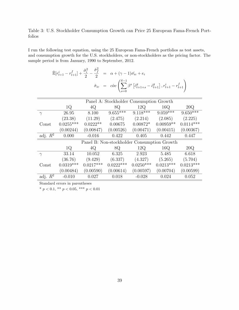
Table 3: U.S. Stockholder Consumption Growth can Price 25 European Fama-French Port-folios

I run the following test equation, using the 25 European Fama-French portfolios as test assets,and consumption growth for the U.S. stockholders, or non-stockholders as the pricing factor. Thesample period is from January, 1990 to September, 2012.

E[rit+1 − rft+1] +

σ2i2−σ2f2

= α+ (γ − 1)σic + ei

σic = ˆcov

(S−1∑s=0

βs[cgt+1+s − c

gt+1

], rit+1 − r

ft+1

)

Panel A: Stockholder Consumption Growth1Q 4Q 8Q 12Q 16Q 20Q

γ 26.95 8.100 9.655*** 9.118*** 9.059*** 9.650***(23.38) (11.29) (2.475) (2.214) (2.085) (2.225)

Const 0.0255*** 0.0222** 0.00675 0.00872* 0.00959** 0.0114***(0.00244) (0.00847) (0.00526) (0.00471) (0.00415) (0.00367)

adj. R2 0.000 -0.016 0.422 0.405 0.442 0.447

Panel B: Non-stockholder Consumption Growth1Q 4Q 8Q 12Q 16Q 20Q

γ 33.14 10.052 6.325 2.923 5.485 6.618(36.76) (9.429) (6.337) (4.327) (5.265) (5.704)

Const 0.0319*** 0.0217*** 0.0222*** 0.0250*** 0.0213*** 0.0213***(0.00484) (0.00590) (0.00614) (0.00597) (0.00704) (0.00599)

adj. R2 -0.010 0.027 0.018 -0.028 0.024 0.052

Standard errors in parentheses

* p < 0.1, ** p < 0.05, *** p < 0.01

39

Table 4: U.S. Stockholder Consumption Growth cannot Price 25 Japanese Fama-FrenchPortfolios

I run the following test equation, using the 25 Japanese Fama-French portfolios as test assets, andconsumption growth for the U.S. stockholders, or non-stockholders as the pricing factor. TheEurope market consists of Austria, Belgium, Denmark, Finland, France, Germany, Greece,Ireland, Italy, the Netherlands, Norway, Portugal, Spain, Sweden, Switzerland, and the UnitedKingdom. The sample period is from January, 1990 to September, 2012.

E[rit+1 − rft+1] +

σ2i2−σ2f2

= α+ (γ − 1)σic + ei

σic = ˆcov

(S−1∑s=0

βs[cgt+1+s − c

gt+1

], rit+1 − r

ft+1

)

Panel A: Stockholder Consumption Growth1Q 4Q 8Q 12Q 16Q 20Q

γ -44.79*** -14.64 -4.988 -2.310 -3.386 -1.985(10.52) (13.16) (5.099) (3.694) (2.724) (2.529)

Const 0.00860*** 0.00278 0.00627 0.00172 0.00514* 0.00351(0.00205) (0.00168) (0.00453) (0.00134) (0.00275) (0.00243)

adj. R2 0.399 0.041 0.022 -0.001 0.043 0.008

Panel B: Non-stockholder Consumption Growth1Q 4Q 8Q 12Q 16Q 20Q

γ 25.86* -4.692 -2.091 -3.662 -5.625 -7.737(15.04) (16.37) (7.388) (4.670) (4.359) (6.743)

Const 0.00222 0.00331 0.00367 0.00661 0.00906 0.00821(0.00164) (0.00753) (0.00693) (0.00560) (0.00533) (0.00543)

adj. R2 0.061 -0.029 -0.035 0.002 0.058 0.049

Standard errors in parentheses

* p < 0.1, ** p < 0.05, *** p < 0.01

40

Table 5: U.S. Stockholder Consumption Growth cannot Price 25 Asia Pacific (ex-Japan)Fama-French Portfolios

I run the following test equation, using the 25 Asian-Pacific (excluding Japan) Fama-Frenchportfolios as test assets, and consumption risk for the US stockholder, or non-stockholder as thepricing factor. The Asia Pacific market consists of Australia, Hong Kong, New Zealand, andSingapore. The sample period is from January, 1990 to September, 2012.

E[rit+1 − rft+1] +

σ2i2−σ2f2

= α+ (γ − 1)σic + ei

σic = ˆcov

(S−1∑s=0

βs[cgt+1+s − c

gt+1

], rit+1 − r

ft+1

)

Panel A: Stockholder Consumption Growth1Q 4Q 8Q 12Q 16Q 20Q

γ -34.64* -12.33 -10.37* -3.504 -8.770** -10.57***(18.74) (8.416) (5.665) (5.233) (3.559) (3.620)

Const 0.0198*** 0.0214*** 0.0323*** 0.0257*** 0.0321*** 0.0331***(0.00220) (0.00184) (0.00512) (0.00432) (0.00349) (0.00388)

adj. R2 0.101 0.086 0.066 -0.015 0.162 0.228

Panel B: Non-stockholder Consumption Growth1Q 4Q 8Q 12Q 16Q 20Q

γ -6.539 -6.894 -11.22 -12.63 -17.37** -7.245(32.47) (17.05) (10.76) (7.962) (7.426) (6.049)

Const 0.0203* 0.0264*** 0.0325*** 0.0388*** 0.0394*** 0.0278***(0.0114) (0.00681) (0.00773) (0.00891) (0.00651) (0.00315)

adj. R2 -0.041 -0.033 0.012 0.064 0.151 -0.003

Standard errors in parentheses

* p < 0.1, ** p < 0.05, *** p < 0.01

41

Tab

le6:

Lab

orIn

com

eof

Sto

ckhol

der

s(%

)

Th

ela

bor

inco

me

and

the

stock

hol

der

stat

us

are

dra

wn

from

Su

rvey

ofC

onsu

mer

Fin

ance

(SC

F).

Ire

port

the

wage

share

of

each

grou

psu

rvey

ed.

Sto

ckh

old

ers

incl

ud

eh

old

ers

of(1

)st

ock

mu

tual

fun

ds,

(2)

bon

dfu

nd

s(e

xcl

ud

ing

Tre

asu

ryan

dM

un

icip

al

bon

d

fun

ds)

,(3

)co

mb

inat

ion

fun

ds

that

hol

db

oth

stock

san

db

ond

s,(4

)al

lot

her

fun

ds

(mu

tual

fun

ds,

hed

ge

fun

ds,

or

RE

ITs

(Rea

l

Est

ate

Inve

stm

ent

Tru

sts)

),(5

)in

div

idu

alst

ock

s.T

op3r

dst

ock

hol

der

sid

enti

fyst

ock

hol

der

sw

hos

est

ock

posi

tion

sare

am

on

g

the

top

thir

dof

the

stock

hol

der

s.

1989

1995

2001

2007

2010

Ave

rage

All

stock

hol

der

s66

.29

73.1

879

.93

79.5

369

.94

Top

3rd

stock

hol

der

s39

.98

54.6

054

.70

55.7

441

.24

48.0

5H

older

sof

fore

ign

indiv

idual

stock

s24

.30

14.7

518

.86

12.2

16.8

2H

older

sof

fore

ign

indiv

idual

stock

san

dal

lm

utu

alfu

nds

49.3

255

.05

61.9

063

.83

54.2

8

Rat

ioof

lab

orin

com

ep

erhou

sehol

dof

the

iden

tified

grou

pto

rest

ofp

opula

tion

All

stock

hol

der

s3.

714.

705.

246.

053.

42T

op3r

dst

ock

hol

der

s5.

128.

597.

188.

426.

92H

older

sof

fore

ign

indiv

idual

stock

s5.

562.

542.

672.

43H

older

sof

fore

ign

indiv

idual

stock

san

dal

lm

utu

alfu

nds

3.19

3.04

4.61

8.14

42

Table 7: Benchmark Calibration: Parameters

Parameters

Mean of Wage Share L0 = 0.75Mean of Dividend Share D0 = 0.25Persistence of Wage ρ = 0.99Persistence of Dividend κ = 0.89Vol of Wage Shock vol(z) = 0.0120Vol of Dividend Shock vol(u) = 0.0065Corr of Wage and Dividend Shock corr(ui, zi) = −0.05Cross Corr of Wage Shock corr(z1, z2) = 0.39Cross Corr of Dividend Shock corr(u1, u2) = 0.13Cross Corr of the Two Shocks corr(ui, zj) = 0.06Non-stockholder EIS σn = 0.1Stockholder EIS σ = 0.3Non-stockholder Risk aversion γn = 10Stockholder Risk aversion γ = 10Discount factor β = 0.985Income Share of Stockholders µ = 0.48Non-stockholder Borrowing Limit bn = −0.39Stockholder Borrowing Limit bs = −0.36

43

Table 8: Benchmark Calibration Results

All data moments are computed at quarterly frequency for the U.S., except for the consumption

correlation. The correlation of the real per capital consumption growth rates is calculated for the

U.S. and U.K. household-level survey data. To be consistent with the empirical results, the 12

quarter correlation of consumption growth rates are reported.

Moments Model Data

Corr(Rsh, R

sf ) 0.84 0.83

Corr(∆Caggh,12Q,∆C

aggf,12Q) 0.33 0.31

Corr(∆Csh,12Q,∆C

sf,12Q) 0.52 0.51

Corr(∆Cnh,12Q,∆C

nf,12Q) 0.24 0.26

Corr(∆Csh,12Q,∆C

nf,12Q) 0.16 0.07

Corr(∆Cnh,12Q,∆C

sh,12Q) 0.76 0.45

Mean of Risk-free rate 1.18% 1.11%Volatility of Risk-free rate 1.12% 1.59%Mean of Equity Risk Premium 4.79% 5.65%Volatility of Stock return 12.05% 17.24%Vol of ∆Cn,i 2.59% 2.14%Vol of ∆Cs,i 2.19% 3.76%V ol(bi) 2.63% 1.71%V ol(∆NetEquityPositioni) 4.25% 2.97%

44

Table 9: The Role of Limited Stock Market Participation

All data moments are computed at quarterly frequency for the U.S., except for the consumptioncorrelation. The correlation of the real per capital consumption growth rates is calculated for theU.S. and U.K. household-level survey data. To be consistent with the empirical results, the 12quarter correlation of consumption growth rates are reported.Column Rep Agent represents the alternative model where there is full participation in the stockmarket in each country. Column Benchmark represents the benchmark model, where there islimited stock market participation.

Moments Rep Agent Bechmark Data

Corr(Rsh, R

sf ) 0.97 0.84 0.83

Corr(∆Caggh,12Q,∆C

aggf,12Q) 0.79 0.33 0.31

Mean of Risk-free rate 4.70% 1.18% 1.11%Volatility of Risk-free rate 0.95% 1.12% 1.59%Mean of Equity Risk Premium 1.00% 4.79% 5.65%Volatility of Stock return 9.22% 12.05% 17.24%V ol(∆Ci,agg) 2.01% 2.18% 2.95%V ol(bi) 0.01% 2.63% 1.71%V ol(∆NetEquityPositioni) 1.63% 4.25% 2.97%

45

Table 10: The Role of Preference Heterogeneity

Moments CRRA Alt. EIS Alt. RA Benchmark Data(0.1, 0.1) (0.3, 0.3) γn = 5 (0.1, 0.3)

Corr(Rsh, R

sf ) 0.94 0.84 0.84 0.84 0.83

Corr(∆Caggh,12Q,∆C

aggf,12Q) 0.48 0.30 0.40 0.33 0.31

Corr(∆Csh,12Q,∆C

sf,12Q) 0.76 0.52 0.63 0.52 0.51

Corr(∆Cnh,12Q,∆C

nf,12Q) 0.23 0.14 0.23 0.24 0.26

Corr(∆Csh,12Q,∆C

nf,12Q) 0.37 0.20 0.19 0.16 0.07

Corr(∆Cnh,12Q,∆C

sh,12Q) 0.77 0.75 0.71 0.76 0.45

Mean of Risk-free rate -0.91% 5.24% 1.13% 1.18% 1.11%Volatility of Risk-free rate 2.95% 1.34% 1.93% 1.12% 1.59%Mean of Equity Risk Premium 5.94% 0.72% 4.79% 4.79% 5.65%Volatility of Stock return 22.70% 12.01% 12.04% 12.05% 17.24%Vol of ∆Cn,i 2.62% 2.76% 2.61% 2.59% 2.14%Vol of ∆Cs,i 1.91% 2.21% 2.19% 2.19% 3.76%V ol(bi) 4.00% 0.05% 2.63% 2.63% 1.71%V ol(∆NetEquityPositioni) 4.52% 4.25 4.25%% 4.25% 2.97%

46

Table 11: Bond Economy Calibration Results

Moments Segmented Integrated Data(Bond) (Benchmark)

Corr(Rsh, R

sf ) 0.25 0.84 0.83

Corr(∆Caggh,12Q,∆C

aggf,12Q) 0.14 0.33 0.31

Corr(∆Csh,12Q,∆C

sf,12Q) 0.12 0.52 051

Corr(∆Cnh,12Q,∆C

nf,12Q) 0.18 0.24 0.26

Corr(∆Csh,12Q,∆C

nf,12Q) 0.09 0.16 0.07

Corr(∆Cnh,12Q,∆C

sh,12Q) 0.70 0.76 0.45

Mean of Risk-free rate 0.027% 1.18% 1.11%Volatility of Risk-free rate 1.84% 1.12% 1.59%Mean of Equity Risk Premium 8.32% 4.79% 5.65%Volatility of Stock return 13.73% 12.05% 17.24%Vol of ∆Cn,i 2.62% 2.59% 2.14%Vol of ∆Cs,i 2.59% 2.19% 3.76%V ol(bi) 2.64% 2.63% 1.71%

47