likelihood based inference on the box-cox family of transformations:
TRANSCRIPT
LIKELIHOOD BASEDINFERENCE ON
THE BOX-COX FAMILY OF
TRANSFORMATIONS:
SAS AND MATLAB PROGRAMS
Scott Hyde
Department of Mathematical Sciences
Montana State University
April 7, 1999
A writing project submitted in partial fulfillmentof the requirements for the degree
Master of Science in Statistics

APPROVAL
of a writing project submitted by
SCOTT HYDE
This writing project has been read by the writing project director and has been foundto be satisfactory regarding content, English usage, format, citations, bibliographicstyle, and consistency, and is ready for submission to the Statistics Faculty.
Date Robert J. BoikWriting Project Director

Contents
1 Introduction 1
1.1 Conventional Linear Model . . . . . . . . . . . . . . . . . . . . . . . . . 1
1.2 Box-Cox Family of Transformations . . . . . . . . . . . . . . . . . . . . 2
2 Estimation of the Transformation Parameter 3
2.1 Derivation of the Log Likelihood Function . . . . . . . . . . . . . . . . 3
3 Newton-Raphson Algorithm 6
4 Confidence Intervals for λ 8
4.1 Asymptotic Distribution of MLE . . . . . . . . . . . . . . . . . . . . . 9
4.2 Inversion of LR Test . . . . . . . . . . . . . . . . . . . . . . . . . . . . 12
5 Examples 13
6 Programming Notes 17
A Appendix 20
A.1 SAS Code . . . . . . . . . . . . . . . . . . . . . . . . . . . . . . . . . . 20
A.2 MATLAB Code . . . . . . . . . . . . . . . . . . . . . . . . . . . . . . . 25
A.3 Finding the limit of ui and vi . . . . . . . . . . . . . . . . . . . . . . . 30
A.4 Finding the form for the observed Fisher’s Total Information matrix. . 31
References 34

Box-Cox MLE computation 1
A SAS program to compute the MLE of theBox-Cox Transformation parameter
Abstract
Box and Cox [3] proposed a parametric family of power transformations of the datato reduce problems with non-normality and heteroscedasticity. This paper presentsprograms in SAS and MATLAB to compute the MLE and to compute approximateconfidence intervals for the Box-Cox transformation parameter.
1 Introduction
1.1 Conventional Linear Model
In the conventional linear model, the response is modeled by a linear combinationof parameters and explanatory variables plus random fluctuation. Additionally, theerrors, or random fluctuation, εj, j = 1, . . . , n are assumed to be independent andnormally distributed with mean 0 and variance σ2. In short,
y = Xβ + ε,
whereε ∼ N(0, σ2I).
Note that y is an n × 1 vector, X is a n × p matrix, and β is a p × 1 vector ofundetermined coefficients.
Box and Cox [3] note that the above model implies several assumptions, namely
1. Linearity of Structure for E(y);
2. Constancy of Error Variances;
3. Normality of Distributions; and
4. Independence of Observations.
Typically, the first and last assumptions are assumed to have been met. But, whenthese assumptions are not met, then conventional methods of inference, prediction,and estimation fail. Procedures are available for examining departures from theseassumptions. If replications are available, then a standard lack of fit test can be
Box-Cox MLE computation 2
performed. The Durbin-Watson test can be used to test for a serial correlation (i.e.,AR(1)).
For the second of the above assumptions, there are several methods for detectingheteroscedasticity. One method consists of examining a plot of the residuals versus thepredicted values. If the residual plot shows random scatter, then there is little evidenceagainst the homogeneity of variance assumption. Nonetheless, this does not imply thathomogeneity is satisfied. Other methods, including the residual plot method, can befound in Chapter 6 of Sen & Srivastava’s textbook [11].
Two methods are prominent for detecting non-normality. These methods, namelyprobability plots and inference tests, also are described in Sen and Srivastava [11].Probability plots are constructed by plotting the data versus quantiles γi of the normaldistribution. More specifically, the ith normal quantile is
γi = Φ−1
(i− 3/8
n + 1/4
).
When plotting γi versus the ordered data, a line should form if the data are normal. Ifthe data are not normal, then other patterns will emerge. Inference tests for normalityinclude the Shapiro-Wilk test, which seems to be the standard for small data sets.Other methods include the square of the correlation between the ordered data and theγi’s, which was initially used as an approximation to the Shapiro-Wilk statistic. Whenn is large, the Kolmogorov test statistic may be used.
If the first three assumptions are not satisfied, then a transformation of the originaldata may help so that methods of inference, prediction, and estimation can be valid.Several different transformation choices have been discussed by various authors. Onemain goal is to attain approximate constant variance. References are given to otherpapers in Box and Cox [3], Hoyle [5], and Sakia [9]. While there are many choicesfor transformations, this paper discusses the Box-Cox transformation of the dependentvariable.
1.2 Box-Cox Family of Transformations
The Box-Cox transformation family introduces a new parameter λ and transforms theresponse, y, to z = y(λ). The transformation is as follows:
z = y(λ) =
yλ − 1
λif λ 6= 0;
ln y if λ = 0.
(1)
The objective of this family of transformations is to produce data which follow anormal distribution more closely than the original data. While this transformationdoes not guarantee that the transformed data are normal, it does reduce problemswith estimation, prediction, and inference.
Box-Cox MLE computation 3
The transformation above can be used only on positive response variables. Onetransformation suggested by Box and Cox [3] which allows for negative data is
y(λ) =
(y + λ2)
λ1 − 1
λ1
if λ1 6= 0;
ln(y + λ2) if λ1 = 0.
The discussion in this paper is based on equation (1).
2 Estimation of the Transformation Parameter
Estimation of λ can be done by Bayesian methods, by likelihood-based methods, or byother methods. One estimator may be chosen over another if one is more robust. Infact, the mle of λ is not robust. A robust estimator of λ was described by Carroll [4].Although the mle of λ is not robust, there are still situations where it is a very goodestimator. For this reason, the mle of λ will be discussed in this paper.
2.1 Derivation of the Log Likelihood Function
Maximum likelihood estimation consists of the following steps. First, the likelihoodfunction is specified. Second, the likelihood function is maximized with respect to theunknown parameters. For the models in this paper, the maximizers (i.e., mles) can beobtained by taking the derivative of the likelihood function, setting the derivative tozero, and solving for the unknown parameters.
To construct the likelihood function, the distribution of the data, y, can be derivedbased on the assumption that the transformed data y(λ) are normal. The density ofthe multivariate normal distribution (with one response variable) can be written inmatrix form as
f(z|β,Σ) =exp
{−1
2(z − µ)′Σ−1(z − µ)
}(2π)
n2 |Σ| 12
,
where z = y(λ).
If linearity of the structure for E(y) (i.e. µ = Xβ) and homogeneity of variance (i.e.Σ = σ2I) are satisfied, then a slightly different density function emerges:
f(z|β, σ2) =exp
{− 1
2σ2 (z −Xβ)′(z −Xβ)}
(2πσ2)n2
.
But, the pdf of y, not z is needed. By multiplying the pdf of z by the Jacobian, thepdf of y is found to be
f(y|β, σ2, λ) =exp
{− 1
2σ2 (z −Xβ)′(z −Xβ)}
(2πσ2)n2
n∏i=1
yλ−1i .
Box-Cox MLE computation 4
Consequently, the log likelihood function is
ln L(β, σ2, λ|y) = − 1
2σ2(z −Xβ)′(z −Xβ)− n
2ln(2πσ2) + (λ− 1)
n∑i=1
ln yi.
The mles of β, σ2, and λ are found by maximizing the log likelihood function.Finding the values of the parameters that maximize the log likelihood is easily doneby doing the maximization separately for each parameter and substituting its mle intothe log likelihood function.
First, the mle of β will be found. Taking the derivative of ln L with respect to β,setting it equal to zero, and solving for β yields
∂ ln L(β, σ2, λ|y)
∂β= − 1
2σ2(−2X ′z + 2X ′Xβ)
set= 0
=⇒ 2X ′Xβ = 2X ′z
=⇒ β = (X ′X)−X ′z,
where (X ′X)− is any generalized inverse of X ′X. Substituting β for β into the loglikelihood function yields
ln L(σ2, λ|y, β) = − 1
2σ2(z −Hz)′(z −Hz)− n
2ln(2πσ2) + (λ− 1)
n∑i=1
ln yi (2)
= − 1
2σ2z′(I −H)z − n
2ln(2πσ2) + (λ− 1)
n∑i=1
ln yi, (3)
where H = X(X ′X)−X ′.
Taking the derivative of (2) with respect to σ2 and solving the resulting equationyields
∂ ln L(σ2, λ|yβ)
∂σ2= − 1
2σ4z′(I −H)z − n
2σ2
set= 0
=⇒ z′(I −H)z
σ4=
n
σ2
=⇒ σ2 =z′(I −H)z
n.
Accordingly, the concentrated log likelihood function is
ln L(λ|y) = ln L(λ|y, β, σ2) = −1
2
nσ2
σ2− n
2ln(2πσ2) + (λ− 1)
n∑i=1
ln yi
= −n
2ln(2πe)− n
2ln(σ2(z)) + (λ− 1)
n∑i=1
ln yi. (4)

Box-Cox MLE computation 5
Equation (4) represents a partially maximized log likelihood function that dependsonly on λ. Therefore, maximizing (4) with respect to λ will complete the estimationproblem. The derivative of ln L(λ|y) can be written as
∂ ln L(λ|y)
∂λ= − n
2σ2
∂σ2(z)
∂λ+
n∑i=1
ln yi,
which, using the chain rule for vectors, can be simplified as
∂ ln L(λ|y)
∂λ= − n
2σ2
(∂z′
∂λ
∂σ2(z)
∂z
)+
n∑i=1
ln yi.
Expressions for ∂z′
∂λand ∂σ2(z)
∂zare necessary to simplify the above expression. Because
z = y(λ), it follows that
∂zi
∂λ= ui =
λyλ
i ln yi − yλi + 1
λ2if λ 6= 0;
(ln yi)2
2if λ = 0
(5)
where, as shown in appendix A.3,
(ln yi)2
2= lim
λ→0
∂zi
∂λ.
It is convenient to arrange these derivatives into a vector:
∂z
∂λ= u,
where u is an n × 1 vector consisting of {ui}. The derivative ∂σ2(λ)∂z
can be found byusing the rule of quadratic forms found in chapter 8 of Schott [10]. The result is
∂σ2(z)
∂z=
1
n
∂z′(I −H)z
∂z=
2(I −H)z
n.
Combining the preceding gives
∂σ2(z)
∂λ=
∂z′
∂λ
∂σ2(z)
∂z
= u′(
2(I −H)z
n
)
=2u′(I −H)z
n.
In summary,
∂ ln L(λ|y)
∂λ= −u′(I −H)z
σ2+
n∑i=1
ln yi. (6)
Solving for λ proves to be difficult. Apparently, there is no closed form solution to thelikelihood equation ∂ ln L(λ|y)
∂λ= 0. Therefore, iterative techniques need to be used. One
such method is the Newton-Raphson algorithm.

Box-Cox MLE computation 6
3 Newton-Raphson Algorithm
The Newton-Raphson algorithm is an iterative method used to find an unconstrainedmaximum or minimum, or to solve an equation. A full motivation of the subject canbe found in chapter 10 of Kennedy and Gentle [6]. A synopsis of the algorithm follows.
Consider a differentiable scalar function f of an n × 1 vector θ. If an exactexpression for the optimizer of f(θ) does not exist, then an approximation for theoptimizer of f(θ) can be derived. First, expand f(θ) in a second order Taylor Seriesabout the vector θ0 (an initial guess):
f(θ) ≈ f(θ0) + g(θ0)(θ − θ0) +1
2(θ − θ0)
′H(θ0)(θ − θ0), (7)
where the gradient function is
g(θ0) =
[∂f
∂θ
]θ=θ0
,
and the Hessian matrix is
H(θ0) =
[∂2f
∂θ ∂θ′
]θ=θ0
.
An approximate optimizer of f(θ) can be found by taking the derivative of the Taylorapproximation of f(θ) with respect to θ, setting it equal to zero, and solving for θ.
By using vector calculus [10], the derivative of (7) becomes
∂f
∂θ= g(θ0) + H(θ0)(θ − θ0)
set= 0.
Solving for θ gives
θ = θ0 −H(θ0)−1g(θ0). (8)
By renaming θ as θ1 in equation (8), an iterative process can be established, and is
θk+1 = θk −H(θk)−1g(θk), (9)
where θk is the kth iteration and θk+1 is the (k + 1)st iteration. Equation (9) shouldbe repeatedly evaluated until convergence to the solution θ. Convergence will occur ata quadratic rate, which is one reason that this algorithm is often used. Nonetheless,if the initial guess is “too far” from the optimizer, then convergence may not occur.So, an “educated”, rather than arbitrary guess should be used. Once convergence hasoccurred, the Hessian matrix can be used to determine whether θ is a local minimizeror maximizer. If H(θ) is positive definite, then θ is a minimizer of f(θ); and if −H(θ)is positive definite, then θ is a maximizer.

Box-Cox MLE computation 7
Applying this general result to finding mles is simple. All that is necessary is iden-tifying f(θ). Either the concentrated likelihood function L(λ|y), or the concentratedlog likelihood function ln L(λ|y) are normally used for f(θ). In this case, estimationproceeds using f(θ) = ln L(λ|y).
Note that g(λ) already has been derived in (6). The Hessian matrix is the onlyremaining component that is needed to apply the Newton-Raphson method.
Before proceeding, two preliminary results are needed. First, define matrices A,B, and C with sizes of m× l, l× r, and p× q respectively. Then the derivative of theproduct AB with respect to C is the mp× rq matrix
∂(AB)
∂C=
(∂A
∂C
)(Iq ⊗B) + (Ip ⊗A)
(∂B
∂C
). (10)
Second, the derivative of the inverse of an v × v nonsingular matrix, A, whoseentries are functions of a p× q matrix C is
∂A−1
∂C= −(Ip ⊗A−1)
(∂A
∂C
)(Iq ⊗A−1). (11)
Using (10), the derivative of (6) with respect to λ′ is found by identifying
A = −u′(I −H)z, B = (σ2)−1, and C = λ′ = λ,
and m = l = r = p = q = 1. Consequently,
∂2 ln L(λ|y)
∂λ2=
(∂A
∂C
)B + A
(∂B
∂C
)
=
(∂ [−u′(I −H)z]
∂λ
)(σ2)−1 − u′(I −H)z
(∂(σ2)−1
∂λ
). (12)
Now, each individual derivative in (12) needs to be computed. To evaluate ∂(σ2)−1
∂λ,
equation (11) is used by identifying
A = (σ2)−1 and C = λ.
Therefore,
∂(σ2)−1
∂λ= −(σ2)−1
(∂σ2
∂λ
)(σ2)−1
= − 1
(σ2)2
(2u′(I −H)z
n
)
= −2u′(I −H)z
n(σ2)2.

Box-Cox MLE computation 8
Finding an expression for∂[−u′(I −H)z]
∂λinvolves the use of (10). Note that
A = −u′, B = (I −H)z, C = λ′ = λ,
m = r = p = q = 1, and l = n. As a result,
∂ [−u′(I −H)z]
∂λ=
(−∂u′
∂λ
)(I −H)z − u′(I −H)
(∂z
∂λ
)
= v′(I −H)z − u′(I −H)u,
where v is the n× 1 vector containing
vi = −∂ui
∂λ=
2− [(λ ln yi)
2 − 2λ ln yi + 2] yλi
λ3if λ 6= 0;
−(ln yi)3
3if λ = 0,
(13)
and, as shown in appendix A.3,
(ln yi)3
3= − lim
λ→0
∂ui
∂λ.
In summary,
∂2 ln L(λ|y)
∂λ2=
(∂ [−u′(I −H)z]
∂λ
)(σ2)−1 − u′(I −H)z
(∂(σ2)−1
∂λ
)
=v′(I −H)z − u′(I −H)u
σ2+ u′(I −H)z
(2u′(I −H)z
n(σ2)2
).(14)
After simplifying (14), the equation of the Hessian can be written as
H(λ) =∂2 ln L
∂λ2=
v′(I −H)z − u′(I −H)u
σ2+
2
n
(u′(I −H)z
σ2
)2
. (15)
In conclusion, the mle of λ can be found using the Newton-Raphson algorithm(9), with the gradient defined in (6), and the Hessian defined in (15).
4 Confidence Intervals for λ
While there are a variety of methods to find confidence intervals for parameters, onlytwo are discussed in this paper. One is based on the asymptotic distribution of mles,whereas the other is based on the inversion of the LR Test. Both yield approximate(1− α)100% confidence intervals.

Box-Cox MLE computation 9
4.1 Asymptotic Distribution of MLE
Finding a confidence interval using the asymptotic distribution of maximum likelihoodestimators is similar to the pivotal method for finding confidence intervals for locationparameters. Let θ be the mle of θ, a p×1 vector of parameters. Because the distributionof θ is asymptotically normal ([7], pg 198), an approximate (1 − α)100% confidenceinterval for one of the parameters in θ can be found using
θi ± z?SE(θi),
where z? is the(1− α
2
)100th percentile of the standard normal distribution, and SE(θi)
is an estimate of the standard error of θi. Once the mle is known, the standard errorsare all that remain in constructing the intervals. By finding the estimates to theparameters of the asymptotic distribution of θ, expressions for the standard errors canbe found as the square root of the diagonal entries of the estimated covariance matrix.First, the distribution of θ will be stated, followed by a derivation of the approximateasymptotic distribution of λ.
Designate the log likelihood function as `(θ | y). Define U as
U =∂`(θ | y)
∂θ,
and denote the observed Fisher’s total information matrix as
J(θ) = −∂U
∂θ′ = −∂2`(θ | y)
∂θ ∂θ′ .
Then Fisher’s total information matrix, J , is defined as
J(θ) = E[J(θ)] = E(UU ′).
The distribution of√
n(θ − θ), as n → ∞, converges to a normal distribution. Inparticular, [
J(θ)
n
] 12 √
n(θ − θ)dist−→ N(0, I), (16)
where J(θ) is Fisher’s total information matrix [7]. Nonetheless, J(θ) is typically not
known, yet by substituting an n− 12 consistent estimator, J (θ)
nfor J (θ)
nin equation
(16), the same result is obtained. Accordingly,
J(θ)12 (θ − θ)
dist−→ N(0, I) and θ·∼ N(θ, J(θ)−1).
In this paper,
θ =
βσ2
λ

Box-Cox MLE computation 10
and
− J(θ) =
∂2`(θ | y)
∂β ∂β′∂2`(θ | y)
∂β ∂σ2
∂2`(θ | y)
∂β ∂λ(∂2`(θ | y)
∂β ∂σ2
)′∂2`(θ | y)
∂(σ2)2
∂2`(θ | y)
∂σ2 ∂λ(∂2`(θ | y)
∂β ∂λ
)′ (∂2`(θ | y)
∂σ2 ∂λ
)′∂2`(θ | y)
∂λ2
(17)
=1
σ2
X ′XX ′(z −Xβ)
σ2−X ′u
(z −Xβ)′X
σ2
(z −Xβ)′(z −Xβ)
σ4− n
σ2−u′(z −Xβ)
σ2
−u′X −(z −Xβ)′u
σ2u′u− v′(z −Xβ)
.
Appendix A.4 gives details about the expression for J(θ).
The square root of the diagonal entries of J(θ)−1 is an estimate of the standarderror for each of the estimators. An estimator for the standard error of λ is of particularinterest and can be found using inverses of partitioned matrices. First, partition −J(θ)as
−J(θ) =1
σ2
X ′XX ′(z −Xβ)
σ2−X ′u
(z −Xβ)′X
σ2
(z −Xβ)′(z −Xβ)
σ4− n
σ2−u′(z −Xβ)
σ2
−u′X −(z −Xβ)′u
σ2u′u− v′(z −Xβ)
=1
σ2
(J(θ)11 J(θ)12
J(θ)21 J(θ)22
).
Then one estimator for Var(λ) is
Var(λ) = σ2(J(θ)22 − J(θ)21
[J(θ)11
]−1J(θ)12
)−1
.
Two problems exists with this estimator of Var(λ). First, J(θ)11 is singular, andsecond, each J(θ)ij matrix depends on unknown parameters. The latter problem can
averted by substituting the mles for β and σ2. The inverse of J(θ)11 does not exist,
but a generalized inverse does exist and J(θ)21
[J(θ)11
]−J(θ)12 does not depend on
the choice of the generalized inverse. Simplifications to J(θ)11 occur because
X ′(z −Xβ)
σ2=
0︷ ︸︸ ︷X ′(I −H) z
σ2= 0,
Box-Cox MLE computation 11
and(z −Xβ)′(z −Xβ)
(σ2)2− n
2σ2=
1
σ2
[nσ2
σ2− n
2
]=
n
2σ2.
Simplified, J(θ)11 becomes (X ′X 0
0 n2σ2
).
One choice for[J(θ)11
]−is (
(X ′X)− 0
0 2σ2
n
).
As a result, J(θ)21
[J(θ)11
]−J(θ)12 simplifies to
=(
u′Xz′(I −H)u
σ2
) (X ′X)− 0
02σ2
n
X ′u
u′(I −H)z
σ2
=(
u′X(X ′X)−2z′(I −H)u
n
) X ′uu′(I −H)z
σ2
= u′ X(X ′X)−X ′︸ ︷︷ ︸H
u +2(u′(I −H)z)2
nσ2,
where u and z are u and z of (5) and (1) in which λ is substituted for λ.
Further, an explicit expression for Var(λ) can be derived:
Var(λ) = σ2(J(θ)22 − J(θ)21
[J(θ)11
]−J(θ)12
)−1
= σ2
[u′u− v′(I −H)z −
(u′Hu +
2(u′(I −H)z)2
nσ2
)]−1
= σ2
[u′(I −H)u− v′(I −H)z − 2(u′(I −H)z)2
nσ2
]−1
= −
v′(I −H)z − u′(I −H)u
σ2+
2
n
(u′(I −H)z
σ2
)2−1
= −H(λ)−1,

Box-Cox MLE computation 12
where H(λ) is given in (15). Accordingly,
SE(λ) =1√
−H(λ).
In conclusion, an approximate (1−α)100% confidence interval for λ can be foundusing
λ± z?SE(λ)
where z? is the(1− α
2
)100th percentile of the standard normal distribution.
4.2 Inversion of LR Test
An alternative method for finding a confidence interval for λ is based on the inversionof the likelihood ratio test of Ho : λ = λ0 vs Ha : λ 6= λ0. All values of λ0 which yielda Fail to Reject decision are included in the confidence interval.
To implement this inversion, the deviance statistic is used. For λ, the deviance isdefined as
D(λ) = −2[`(λ | y)− `(λ | y)
],
where `(λ | y) is the concentrated log likelihood function given in (4). The deviancehas an asymptotic χ2 distribution [7]. More specifically, if Ho is true, then
D(λ)dist−→ χ2
1,
as n →∞/ Thus, a (1− α)100% confidence interval for λ can be found by solving
D(λ) = χ21−α,1 (18)
for λ. A graphical description of the confidence interval is displayed in Figure 1.
The values of λ which solve (18) can be found using the Newton-Raphson algorithmfor roots given in chapter 5 of Kennedy and Gentle [6]. The equation to solve is
f(λ) = `(λ | y)− `(λ | y) +1
2χ2
1−α,1 = 0.
Here f ′(λ) = ∂`(λ|y)
∂λ, and is given by equation (6). Thus, the iterative equation for
solving for λ is
λk+1 = λk −f(λk)
f ′(λk).
To implement this algorithm, initial guesses are required. The endpoints of theconfidence interval generated by the asymptotic distribution given in the last sectionwork well.

Box-Cox MLE computation 13
−2 −1.5 −1 −0.5 0 0.5 1 1.5−5
0
5
10
15
λ
Devia
nce
χ2.95,1
= 3.8415
Lower bound
mle
Upper bound
Confidence Interval Construction with LRT Test
Figure 1: Matlab plot illustrating inversion of LRT confidence interval
5 Examples
To demonstrate the SAS and MATLAB programs, three data sets will be used. Thefirst data set comes from Neter, Wasserman and Kutner [8]. Measurements of theplasma level of polyamine for 25 healthy children with varying ages were taken.
The general SAS program is given in Appendix A.1. To use the program for thisdata set, several modifications of the program are required. The correct filename andvariable names in the input statement should be specified in the data step:
data in;
infile ’dataplasma’;
input age plasma;

Box-Cox MLE computation 14
Next, the model should be specified in the glmmod procedure. The model is specifiedin the same manner as in the glm procedure. The model for the Neter data is a oneway classification. The modified code is
proc glmmod outdesign=design noprint;
class age;
model plasma = age;
run;
The last thing to change or omit is the title2 statement in the gplot procedure. TheSAS Box-Cox transformation program produces the following output:
OUTPUT
ML Estimate -0.43576
Lower Bound -1.14820
Upper Bound 0.21272
Bounds are based on an approximate 95% Confidence Interval
Using the theoretical result that -2[loglik(lambda0) - loglik(mle)]
is distributed approximately as a one degree of freedom chi-squared
random variable when the null hypotheses (lambda=lambda0) is true.
Neter reported the mle for λ to be between −.4 and −.5, which is consistent with theSAS result. Because the 95% confidence interval given above does not contain 1, theLR test concludes that a transformation is needed. A plot of ln L(λ|y) versus λ isshown in Figure 2. The SAS code to produce this plot is in Appendix A.1.
The second example is a biological experiment using a 3× 4 factorial design withreplication, and can be found in Box and Cox [3]. The two factors in this experimentare poisons with three levels and treatments with four levels. Every combination ofpoison and treatments was assigned to four animals. The survival time for each animalwas recorded. Because this is a two way classification with no interaction, the modelstatement is
proc glmmod outdesign=design noprint;
class poison treatment;
model survival = poison treatment;
run;
When run initially, the SAS program gives an overflow error and does not converge.Changing the initial guess enables the program to converge. From a starting point ofλ = .5, SAS generates
Box-Cox MLE computation 15
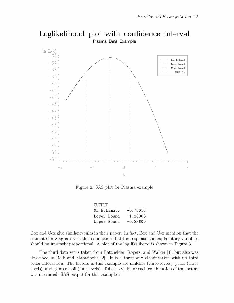
Figure 2: SAS plot for Plasma example
OUTPUT
ML Estimate -0.75016
Lower Bound -1.13803
Upper Bound -0.35609
Box and Cox give similar results in their paper. In fact, Box and Cox mention that theestimate for λ agrees with the assumption that the response and explanatory variablesshould be inversely proportional. A plot of the log likelihood is shown in Figure 3.
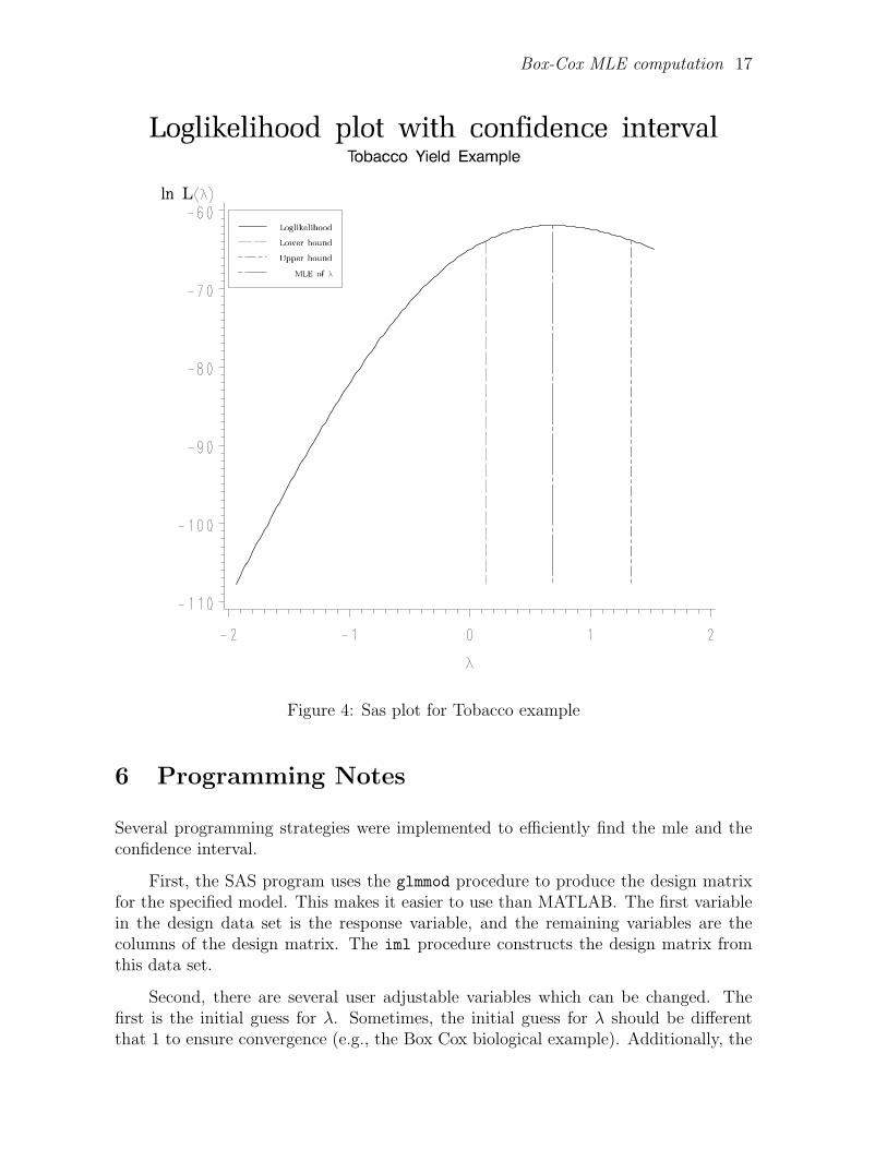
The third data set is taken from Batchelder, Rogers, and Walker [1], but also wasdescribed in Boik and Marasinghe [2]. It is a three way classification with no thirdorder interaction. The factors in this example are mulches (three levels), years (threelevels), and types of soil (four levels). Tobacco yield for each combination of the factorswas measured. SAS output for this example is

Box-Cox MLE computation 16
Figure 3: SAS plot for biological experiment
OUTPUT
ML Estimate 0.68951
Lower Bound 0.13732
Upper Bound 1.34040
This corresponds exactly to the results published in Boik and Marasinghe [2]. A graphof the log likelihood is displayed in Figure 4.
Using MATLAB is more difficult than using SAS because it is more tedious tospecify the design matrix. Nonetheless, the matlab commands dummyvar and x2fx arehelpful when generating design matrices. In fact, results for some simple models caneasily be constructed. Figure 5 shows the corresponding output for the plasma data.MATLAB code is given in Appendix A.2.
Box-Cox MLE computation 17
Figure 4: Sas plot for Tobacco example
6 Programming Notes
Several programming strategies were implemented to efficiently find the mle and theconfidence interval.
First, the SAS program uses the glmmod procedure to produce the design matrixfor the specified model. This makes it easier to use than MATLAB. The first variablein the design data set is the response variable, and the remaining variables are thecolumns of the design matrix. The iml procedure constructs the design matrix fromthis data set.
Second, there are several user adjustable variables which can be changed. Thefirst is the initial guess for λ. Sometimes, the initial guess for λ should be differentthat 1 to ensure convergence (e.g., the Box Cox biological example). Additionally, the

Box-Cox MLE computation 18
−2 −1.5 −1 −0.5 0 0.5 1 1.5−52
−50
−48
−46
−44
−42
−40
−38
−36
−1.1482
0.21272
−0.43576
λ
Lo
g lik
elih
oo
d
Approximate 95%CI for λ for the Plasma data
Figure 5: Matlab plot for Plasma data
confidence level can be changed if a confidence interval other than 95% is desired. Thevariables small and tol can be specified according to the user’s preferences.
The last strategy implemented was using the full rank singular value decompositionto save on memory storage. Many of the quadratic forms derived include the matrixI − H (e.g. v′(I − H)u). Rather than forming the n × n matrix I − H , H isdecomposed into
H = X(X ′X)−X ′ = X
(X ′X)−︷ ︸︸ ︷SD−1S′ X ′ =
F︷ ︸︸ ︷XSD− 1
2
F ′︷ ︸︸ ︷D− 1
2 S′X ′ = FF ′,
where D is an r×r diagonal matrix with non-negative entries, S is an n×r matrix, andr = rank(X). As a result, F is an n × r matrix. By factoring H this way, quadratic

Box-Cox MLE computation 19
forms can be rewritten as
v′(I −H)u = v′(I − FF ′)u = v′u− (v′F )(F ′u).
This reduces the storage space from n2 to nr. Because r is typically much smaller thann, this saves a relatively large amount of space.

Box-Cox MLE computation 20
A Appendix
A.1 SAS Code
To execute this code on a different data set, the following changes are required. First,in the data statements, the infile filename, the input variable names, and the modelspecified in proc glmmod must be modified appropriately.
Second, the user defined variables can be changed. The initial guess for λ mayneed to be different than 1 in order for convergence of the estimate. Also, changes inthe confidence level are made here.
Third, in the gplot procedure, any number of changes can be made, with theminimum being the title2 statement, which should be suitably changed.
dm ’log;clear;out;clear;’; /*This clears the log and output windows*/
/*SAS program for finding the maximum likelihood estimate of the */
/*Box-Cox transformation parameter assuming normality of the */
/*transformed data and homogeneity of variance */
/*===============================================================*/
data in;
infile ’datatobacco’;
input mulch year soil response;
/* proc glmmod is used only to construct the design matrix, which*/
/* is used in proc iml. You will need to specify the model in */
/*proc glmod. Only one response variable can be used. */
proc glmmod outdesign=design noprint;
class mulch year soil;
model response = mulch year soil
mulch*year mulch*soil year*soil;
run;
/*===============================================================*/
proc iml;
/*This section of the code breaks up the data set, design, */
/*into the response variable (y) and the design matrix (X) */
use design;
names = contents();
p = nrow(names);
response = names[1,];
dematrix = names[2:p,1];
read all var response into y;

Box-Cox MLE computation 21
read all var dematrix into X;
n=nrow(X);
/*=======================================================================*/
/*User Adjustable variables*/
lam = 1; /*Initial guess for the mle of lambda. */
ConLevel = .95; /*Specify the Confidence Level here. */
small = 1.e-10; /*Numbers smaller than this are zero. */
tol = 1.e-10; /*Estimate error tolerances. */
/*=======================================================================*/
/* Constants used throughout the program */
XPX = X‘*X;
call svd(UU,QQ,V,XPX);
r = max(loc(QQ>small)); /*rank of XPX*/
U = UU[,1:r];
Q = QQ[1:r];
F = X*U*diag(Q##-.5); /*Note that H = X*ginv(X‘*X)*X‘ = F*F‘*/
free UU U QQ Q V XPX; /*Free the space. These won‘t be used again.*/
pi = arcos(-1); /*This is pi*/
logy = log(y);
slogy = logy[+]; /*Sum of the logy‘s*/
one = J(n,1);
/* This loop generates both the maximum likelihood estimate of lambda*/
/* and the ConLevel*100% confidence interval for lambda. */
do i = 1 to 3;
step = 1;
if i = 2 then
do;
const = -n/2*(log(2*pi) + 1)-slogy-loglik+cinv(ConLevel,1)/2;
iguess = probit((1+ConLevel)/2)*sqrt(-1/H);
end;
/*This statement chooses the initial guesses for finding the lower*/
/*and upper bound on lambda*/
if i ^= 1 then
if i=2 then lam = mlelam - iguess;
else lam = mlelam + iguess;
do until(abs(step) < tol);
if abs(lam) < small then /*This specifies the limit of Z, U, and V*/
do; /*when lambda approaches zero (undefined */
Z=logy; /*otherwise). */
U=logy##2/2;
if i=1 then V=-logy##3/3;
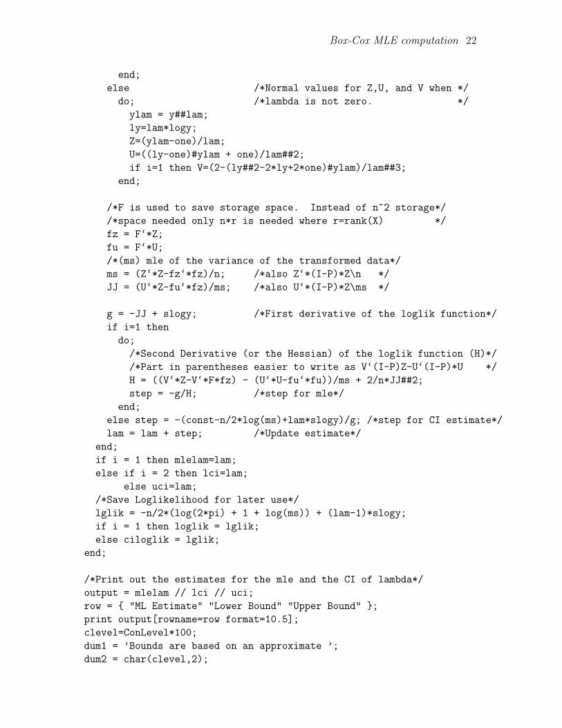
Box-Cox MLE computation 22
end;
else /*Normal values for Z,U, and V when */
do; /*lambda is not zero. */
ylam = y##lam;
ly=lam*logy;
Z=(ylam-one)/lam;
U=((ly-one)#ylam + one)/lam##2;
if i=1 then V=(2-(ly##2-2*ly+2*one)#ylam)/lam##3;
end;
/*F is used to save storage space. Instead of n^2 storage*/
/*space needed only n*r is needed where r=rank(X) */
fz = F‘*Z;
fu = F‘*U;
/*(ms) mle of the variance of the transformed data*/
ms = (Z‘*Z-fz‘*fz)/n; /*also Z‘*(I-P)*Z\n */
JJ = (U‘*Z-fu‘*fz)/ms; /*also U‘*(I-P)*Z\ms */
g = -JJ + slogy; /*First derivative of the loglik function*/
if i=1 then
do;
/*Second Derivative (or the Hessian) of the loglik function (H)*/
/*Part in parentheses easier to write as V‘(I-P)Z-U‘(I-P)*U */
H = ((V‘*Z-V‘*F*fz) - (U‘*U-fu‘*fu))/ms + 2/n*JJ##2;
step = -g/H; /*step for mle*/
end;
else step = -(const-n/2*log(ms)+lam*slogy)/g; /*step for CI estimate*/
lam = lam + step; /*Update estimate*/
end;
if i = 1 then mlelam=lam;
else if i = 2 then lci=lam;
else uci=lam;
/*Save Loglikelihood for later use*/
lglik = -n/2*(log(2*pi) + 1 + log(ms)) + (lam-1)*slogy;
if i = 1 then loglik = lglik;
else ciloglik = lglik;
end;
/*Print out the estimates for the mle and the CI of lambda*/
output = mlelam // lci // uci;
row = { "ML Estimate" "Lower Bound" "Upper Bound" };
print output[rowname=row format=10.5];
clevel=ConLevel*100;
dum1 = ’Bounds are based on an approximate ’;
dum2 = char(clevel,2);
Box-Cox MLE computation 23
dum3 = ’% Confidence Interval ’;
_ = concat(dum1,concat(dum2,dum3));
print _;
print ’Using the theoretical result that -2[loglik(lambda0) - loglik(mle)]’;
print ’is distributed approximately as a one degree of freedom chi-squared’;
print ’random variable when the null hypotheses (lambda=lambda0) is true. ’;
/*The following statements form the data for a graph of the Log-likelihood */
/*function along with the (ConLevel*100)% Conifidence Interval */
spread = (uci-lci)/6; /* approximate spread */
maxci=max(abs(lci),abs(uci));
lbs = -maxci-3*spread; /* Lowerbound for plot */
ubs = maxci+spread; /* Upperbound for plot */
ss = spread/10; /* Stepsize for plot */
/*Generation of the data is here in the do loop*/
do lam = lbs to ubs by ss;
if abs(lam) < small then
Z = logy;
else
Z = (y##lam-1)/lam;
ms = (Z‘*Z-Z‘*F*F‘*Z)/n; /*ms=Z‘(I-H)Z\n*/
lglik = -n/2*(log(2*pi) + 1 + log(ms)) + (lam-1)*slogy;
dummy = dummy // ( lam || lglik || 1 );
end;
/*The next four lines form the data for plotting the confidence interval*/
/*and the mle */
miny = min(dummy[,2]);
dummy = dummy // ( lci || ciloglik || 2 ) // (lci || miny || 2);
dummy = dummy // ( uci || ciloglik || 3 ) // (uci || miny || 3);
dummy = dummy // ( mlelam || loglik || 4) // (mlelam || miny || 4);
create plotdata from dummy [ colname = { Lambda LogLikel graph } ];
append from dummy;
close plotdata;
/*This is the main SAS code for doing the Plot of the */
/*Log Likelihood Function*/
/* goptions device=psepsf gsfname=temp gsflen=132 hsize=6in vsize=6in
gsfmode=replace; */
symbol1 color=black interpol=join width=2 value=none height=3;
symbol2 color=green interpol=join width=2 value=none line=4 height=3;
symbol3 color=red interpol=join width=2 value=none line=8 height=3;
symbol4 color=red interpol=join width=2 value=none line=10 height=3;
axis1 label=(font=greek ’l’);

Box-Cox MLE computation 24
axis2 label=(font=centx ’ln L’ font=greek ’(l)’);
legend across=1 position=(top inside left) label=none cborder=black
value=(font=zapf height=.5 tick=1 ’Loglikelihood’ tick=2 ’Lower bound’
tick=3 ’Upper bound’ tick=4 ’MLE of ’ font=greek ’l’) mode=protect
shape=symbol(3,1);
proc gplot data=plotdata;
plot LogLikel*Lambda=graph /legend=legend1 haxis=axis1 vaxis=axis2;
title font=zapf ’Loglikelihood plot with confidence interval’;
/*===============================================================*/
title2 font=swiss ’Subtitle’;
/*===============================================================*/
run;
quit;

Box-Cox MLE computation 25
A.2 MATLAB Code
The MATLAB function below requires the design matrix, the response variable, andthe confidence level. A fourth input argument can be given to change the initial guessfor λ. If left out, λ = 1 will be used. The function returns λ, the upper and lowerendpoints of the confidence interval, ln L(λ), plus the transformed estimates of theresponse, β, and σ2. The MATLAB command
[mlelam,lci,uci] = box(X,y,ConLevel)
will return only λ, and the confidence intervals. The function also plots the log likeli-hood function.
function [mlelam,lci,uci,loglik,Zmle,Bmle,mSmle] = box(X,y,ConLevel,lam)
% Scott Hyde December 27, 1998
% Matlab program for finding the maximum likelihood estimate of the
% Box-cox transformation parameter assuming normality of the transformed data
% and homogeneity of variance
%
% Inputs
% X (the design matrix)
% y (the data vector (response variable))
% ConLevel (Specify the (Conlevel*100)% confidence level to be found
% lam (Initial guess for mle) (if not given, default is 1)
%
% Outputs
% mlelam
% lci, uci (upper and lower limits for an approximate ConLevel CI for lambda
% loglik (the associated log likelihood)
% Zmle (transformed data)
% Bmle (transformed estimates of the parameters)
% mSmle (transformed common variance)
%
[n,p] = size(y);
% User Adjustable variables
if nargin == 3,
lam = 1; %Initial guess for mle of lambda if not
end; %specified.
small = 1.e-10; %Numbers smaller than this are zero.
tol = 1.e-10; %Number of decimal places of accuracy.
%Constants used everywhere
XPX = X’*X;

Box-Cox MLE computation 26
[U,Q,V] = svd(XPX);
q=diag(Q);
r = rank(XPX);
G = U(:,1:r)*diag(q(1:r).^-.5); %Note that pinv(X’*X) = G*G’;
F=X*G; %Note that H = X*pinv(X’*X)*X’ = F*F’
logy = log(y);
slogy = sum(logy);
%---------------------------------------------------------------------
%This loop generates both the maximum likelihood estimate of lambda
%and the approximate ConLevel*100% confidence interval for lambda
%(generated by inverting the likelihood ratio test).
%---------------------------------------------------------------------
for i = 1:3
step = 1;
if i == 2
%const includes the parts of the deviance that are constant, which
%makes programming the solution to -2[l(lam) - l(mle(lam))] =
%chi2inv(Conlevel,1) easier. Chi2inv(Conlevel,1) is the ConLevel th
%percentile of the Chi-squared dist with 1 df.
const = -n/2*(log(2*pi)+1)-slogy-loglik+chi2inv(ConLevel,1)/2;
%Since (mlelam - lam) is approx dist as N(0,v) where v=-1/H, then
%good starting values to begin the iteration to find the confidence
%interval are mlelam +- cv*sqrt(v)
iguess = norminv((1+ConLevel)/2,0,1)*sqrt(-1/H);
end;
if i ~= 1
if i == 2
lam = mlelam - iguess; %Initial guess for lower confidence bound
else
lam = mlelam + iguess; %Initial guess for upper confidence bound
end;
end;
while abs(step) > tol,
%preliminary computations
if abs(lam) < small
Z = logy; %These specify the limit of Z, U, and V
U = logy.^2/2; %when lamda approaches zero. (Undefined
if i==1 %otherwise)
V = logy.^3/3;
Box-Cox MLE computation 27
end;
else
Z = (y.^lam-1)/lam; %When lamda is not zero, these are the
ly = lam*logy; %computations for Z, U, and V.
U = ((ly-1).*y.^lam + 1)/lam.^2;
if i==1
V = (2-(ly.^2-2*ly+2).*y.^lam)/lam.^3;
end;
end;
%F is used to save storage space. Instead of n^2 storage space needed
%only n*r is needed where r=rank(X). (r is usually substatially less
%than n)
fz = F’*Z;
fu = F’*U;
%mS is the mle of the variance of the transformed data.
mS = (Z’*Z-fz’*fz)/n; %also Z’*(I-P)*Z/n
JJ = (U’*Z-fu’*fz)/mS; %also U’*(I-P)*Z/mS
g = -JJ + slogy; %First derivative of loglik function
if i == 1
%Second Derivative (or the Hessian) of the loglik function
%Part in parentheses easier to write as V‘(I-P)Z-U‘(I-P)*U
H = ((V’*Z-V’*F*fz) - (U’*U-fu’*fu))/mS + 2/n*JJ.^2;
step = -g/H; %Step for mle
else
step = -(const-n/2*log(mS)+lam*slogy)/g; %Step for CI estimates
end;
lam = lam + step; %Update Estimate
end;
%First loop saves mlelam, second loop, the lci, and third, the uci
switch i
case 1, mlelam = lam;
case 2, lci = lam;
case 3, uci = lam;
end;
lglik = -n/2*(log(2*pi) + 1 + log(mS)) + (lam-1)*slogy;
%Save mles of beta, sigma^2 and transformed data
%Also, save loglikelihood for later use
if i == 1
Bmle = G*G’*(X’*Z); %Estimate of parameters
mSmle = mS;

Box-Cox MLE computation 28
Zmle = Z;
loglik = lglik;
else
ciloglik = lglik;
end;
end;
%-------------------------------------------------------------------
% Graph the Loglikelihood along with the (ConLevel*100)% confidence interval
spread = (uci-lci)/6;
maxci = max(abs(uci),abs(lci));
x=(-(maxci+3*spread)):spread/2:(maxci+spread);
f=[];
[dum,p] = size(x);
% Get the data ready for plotting.
for i=1:p
if abs(x(i)) < small
Z = logy;
else
Z = (y.^x(i)-1)/x(i);
end;
ms = (Z’*Z-Z’*F*F’*Z)/n;
lglik = -n/2*(log(2*pi) + 1 + log(ms)) + (x(i)-1)*slogy;
f = [ f , lglik ];
end;
plot(x,f); %plot the data
ax = axis; %axis parameters
lciline = [ lci ax(3) ; lci ciloglik ];
uciline = [ uci ax(3) ; uci ciloglik ];
mleline = [ mlelam ax(3) ; mlelam loglik ];
line(lciline(:,1),lciline(:,2)); %plot lower ci line
line(uciline(:,1),uciline(:,2)); %plot upper ci line
line(mleline(:,1),mleline(:,2)); %plot mle line
middle = (ax(3)+ax(4))/2;
ysprd = (ax(4)-ax(3))/60;
text(lci+spread/4,middle+10*ysprd,num2str(lci)); %print lci on graph
text(uci+spread/4,middle-10*ysprd,num2str(uci)); %print uci on graph
text(mlelam+spread/4,loglik+ysprd,num2str(mlelam)); %print mle on graph
xlabel(’\lambda’);
ylabel(’Log likelihood’);
endgraph=’CI for \lambda for the Plasma data’
[titlegraph, errmg] = sprintf(’Approximate %2.5g%%’,ConLevel*100);
titlegraph = strcat(titlegraph,endgraph);
title(titlegraph);

Box-Cox MLE computation 29
Box-Cox MLE computation 30
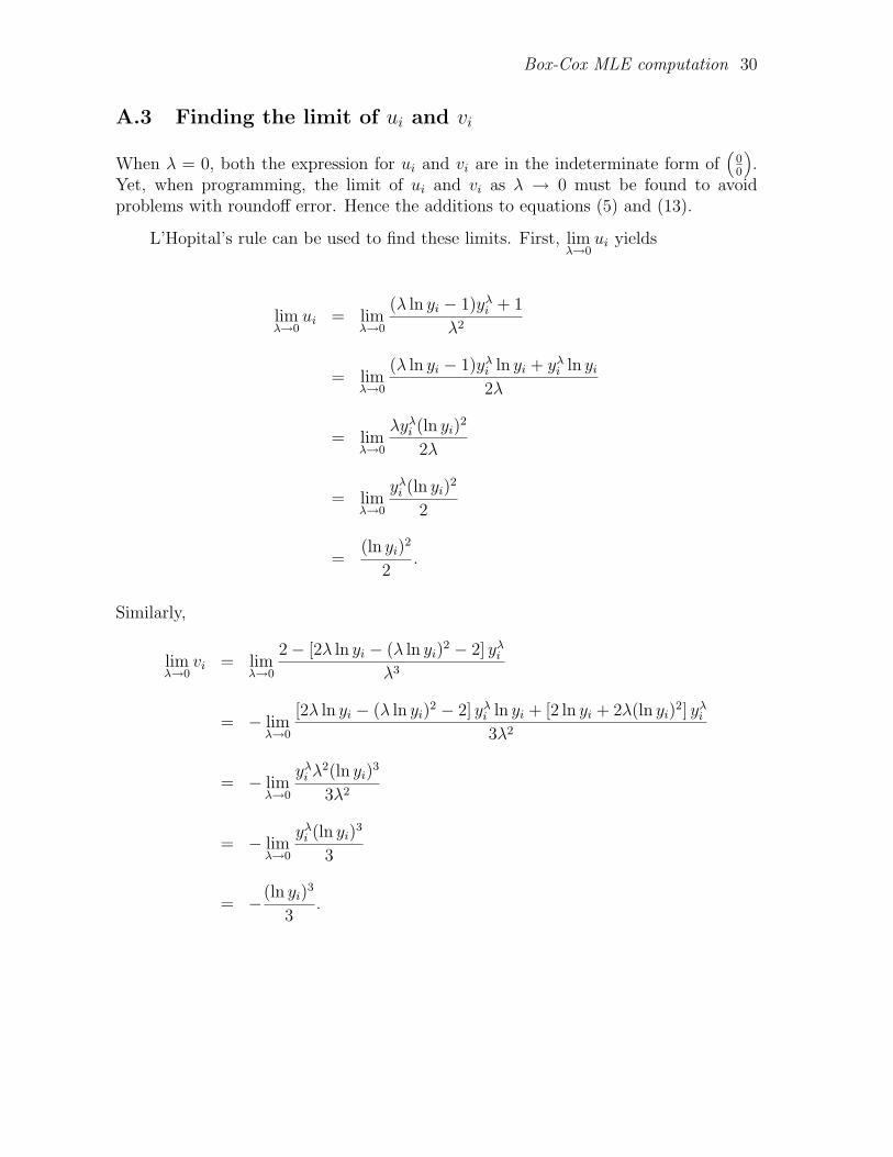
A.3 Finding the limit of ui and vi
When λ = 0, both the expression for ui and vi are in the indeterminate form of(
00
).
Yet, when programming, the limit of ui and vi as λ → 0 must be found to avoidproblems with roundoff error. Hence the additions to equations (5) and (13).
L’Hopital’s rule can be used to find these limits. First, limλ→0
ui yields
limλ→0
ui = limλ→0
(λ ln yi − 1)yλi + 1
λ2
= limλ→0
(λ ln yi − 1)yλi ln yi + yλ
i ln yi
2λ
= limλ→0
λyλi (ln yi)
2
2λ
= limλ→0
yλi (ln yi)
2
2
=(ln yi)
2
2.
Similarly,
limλ→0
vi = limλ→0
2− [2λ ln yi − (λ ln yi)2 − 2] yλ
i
λ3
= − limλ→0
[2λ ln yi − (λ ln yi)2 − 2] yλ
i ln yi + [2 ln yi + 2λ(ln yi)2] yλ
i
3λ2
= − limλ→0
yλi λ2(ln yi)
3
3λ2
= − limλ→0
yλi (ln yi)
3
3
= −(ln yi)3
3.

Box-Cox MLE computation 31
A.4 Finding the form for the observed Fisher’s Total Infor-mation matrix.
To construct the observed Fisher’s Total Information matrix,J(θ), the second partialderivatives of `(θ | y) are needed. Recall
`(θ | y) = − 1
2σ2(z −Xβ)′(z −Xβ)− n
2ln(2πσ2) + (λ− 1)
n∑i=1
ln yi
= − 1
2σ2(z′z − z′Xβ − β′X ′z − β′X ′Xβ)− n
2ln(2πσ2) + (λ− 1)
n∑i=1
ln yi.
Taking the first partial derivatives yields
∂`(θ | y)
∂β= − 1
2σ2(−X ′z −X ′z + 2X ′Xβ)
= − 1
σ2(−X ′z + X ′Xβ),
∂`(θ | y)
∂σ2=
1
2σ4(z −Xβ)′(z −Xβ)− n
2σ2,
and
∂`(θ | y)
∂λ= − 1
2σ2
∂(z −Xβ)′(z −Xβ)
∂λ+
n∑i=1
ln yi
= − 1
2σ2
∂z′
∂λ
∂ [(z′z − z′Xβ − β′X ′z − β′X ′Xβ)]
∂z+
n∑i=1
ln yi
= − 1
2σ2u′(2z − 2Xβ) +
n∑i=1
ln yi
= − 1
σ2u′(z −Xβ) +
n∑i=1
ln yi.
Second partial derivatives are
∂2`(θ | y)
∂β′ ∂β= −X ′X
σ2,
∂2`(θ | y)
∂σ2 ∂β=
1
σ4(−Xz + X ′Xβ)
= −X ′(z −Xβ)
σ4,

Box-Cox MLE computation 32
∂2`(θ | y)
∂λ ∂β=
1
σ2
∂(Xz)
∂λ
=1
σ2
∂z′
∂λ
∂(Xz)
∂z
=u′X
σ2=
X ′u
σ2,
∂2`(θ | y)
∂(σ2)2= − 1
σ6(z −Xβ)′(z −Xβ) +
n
2σ4,
∂2`(θ | y)
∂λ ∂σ2=
1
2σ4
∂(z −Xβ)′(z −Xβ)
∂λ
=1
2σ4[2u′(z −Xβ)]
=u′(z −Xβ)
σ4,
and
∂2`(θ | y)
∂λ2=
1
σ2
product rule︷ ︸︸ ︷∂ [−u′(z −Xβ)]
∂λ
=1
σ2
[−∂u′
∂λ(z −Xβ)− u′∂(z −Xβ)
∂λ
]
=v′(z −Xβ)− u′u
σ2.
Now, recall,
−J(θ) =
∂2`(θ | y)
∂β′ ∂β
∂2`(θ | y)
∂σ2 ∂β
∂2`(θ | y)
∂λ ∂β(∂2`(θ | y)
∂σ2 ∂β
)′∂2`(θ | y)
∂(σ2)2
∂2`(θ | y)
∂λ ∂σ2(∂2`(θ | y)
∂λ ∂β
)′ (∂2`(θ | y)
∂λ ∂σ2
)′∂2`(θ | y)
∂λ2
.

Box-Cox MLE computation 33
So substituting in the second partials results in
=1
σ2
X ′XX ′(z −Xβ)
σ2−X ′u
(X ′(z −Xβ)
σ2
)′(z −Xβ)′(z −Xβ)
σ4− n
σ2−u′(z −Xβ)
σ2
(−X ′u)′
(−u′(z −Xβ)
σ2
)′
u′u− v′(z −Xβ)
,
which is equivalent to equation (17).

Box-Cox MLE computation 34
References
[1] Batchelder, A. R. , Rogers, M. J. , & Walker, J. P. (1966). Effects of SubsoilManagement Practices on Growth of Flue-Cured Tobacco. Agronomy Journal, 58345–347. 15
[2] Boik, R. J. & Marasinghe, M. G. (1989). Analysis of Nonadditive Multiway Clas-sifications. Journal of the American Statistical Association, 84 1059–1064. 15,16
[3] Box, G. E. P. & Cox, D. R. (1964). An Analysis of Transformations. Journal ofthe Royal Statistical Society, 2 211–252. 1, 2, 3, 14
[4] Carroll, R. J. (1980). A Robust Method for Testing Transformations to AchieveApproximate Normality. Journal of the Royal Statistical Society 42 71–78. 3
[5] Hoyle, M. H. (1973). Transformations–An Introduction and a Bibliography. Sta-tistical Review, 41 203–223. 2
[6] Kennedy, W. J. & Gentle, J. E. (1980). Statistical Computing. New York: MarcelDekker. 6, 12
[7] Lindsey, J. K. (1996). Parametric Statistical Inference. New York: Oxford Univer-sity Press. 9, 12
[8] Neter, J., Wasserman, W., & Kutner, M. H. (1990). Applied Linear StatisticalModels, Third Edition. Boston: R. R. Donnelly Sons & Company. 13
[9] Sakia, R. M. (1992). The Box-Cox Transformation Technique: A Review. TheStatistician, 41 169–178. 2
[10] Schott, J. R. (1997). Matrix Analysis For Statistics. New York: John Wiley &Sons. 5, 6
[11] Sen, A. K. & Srivastava, M. S. (1990). Regression Analysis: Theory, Methods, andApplications. New York: Springer-Verlag. 2