Life-Cycle Human Capital Accumulation Across

Countries: Lessons From U.S. Immigrants

David Lagakos, UCSD and NBER

Benjamin Moll, Princeton and NBER

Tommaso Porzio, Yale

Nancy Qian, Yale and NBER

Todd Schoellman, ASU

August, 2016

Abstract

How much does life-cycle human capital accumulation vary across countries? This paper

seeks to answer this question by studying U.S. immigrants, who come from a wide variety of

countries but work in a common labor market. We document that returns to experience accu-

mulated in their birth country are higher for workers coming from rich countries than for those

coming from poor countries. To understand this fact we build a model of life-cycle human capital

accumulation that features three potential theories, working respectively through cross-country

differences in: human capital accumulation, selection, and skill loss. To distinguish between the-

ories, we use new data on the characteristics of immigrants and non-migrants from a large set

of countries. We conclude that the most likely theory is that immigrants from poor countries

accumulate relatively less human capital in their birth countries before migrating. Our findings

imply that life-cycle human capital stocks are on average much larger in rich countries than poor

countries.

Email: lagakos@ucsd.edu, moll@princeton.edu, tommaso.porzio@yale.edu, nancy.qian@yale.edu, todd.schoellman@gmail.com.

For helpful comments we thank Rachel Friedberg, Gordon Hanson, Pete Klenow, Gary Becker, Bob Lucas, Christos

Makridis, two anonymous referees and seminar participants at Houston, MIT, Ottawa, Konstanz, Mannheim, Oxford, and

especially the conference honoring the life and work of Gary Becker at the Becker-Friedman Institute in Chicago. We

thank Caleb Johnson for excellent research assistance. All potential errors are our own.

1. Introduction

How important is human capital in accounting for aggregate income differences across countries?

A large literature on development accounting has concluded that the answer is “only somewhat.”

Specifically, the seminal work of Klenow and Rodrıguez-Clare (1997), Hall and Jones (1999) and

Caselli (2005) finds that human capital stocks vary by roughly a factor of two between the richest and

poorest countries, whereas actual output per worker varies by a factor of more than twenty.

One reason the existing literature has found such a modest role for human capital is that it has fo-

cused largely on human capital accumulated in schooling. Several previous studies have included

human capital accumulated over the life cycle, i.e. after finishing schooling, but have found that it

did not improve the explanatory power of human capital (Klenow and Rodrıguez-Clare, 1997; Bils

and Klenow, 2000, 1998). The data underlying this conclusion came from the Mincer estimates of

Psacharopoulos (1994), which show no systematic variation across countries in either the returns to

potential experience or the average level of potential experience. As a result, researchers using these

data concluded that human capital differences from potential experience must be negligible.1

In contrast, a recent literature has argued that workers in rich countries accumulate much more human

capital over the life cycle than their counterparts in poor countries. Manuelli and Seshadri (2015)

show that this conclusion arises out of a standard Ben-Porath model of human capital accumulation, as

workers in rich countries are able to devote more goods inputs (e.g. books and computers) to their time

spent accumulating human capital. Empirically, Lagakos, Moll, Porzio, Qian, and Schoellman (2016)

use micro-level wage data from a large set of countries to document that returns to potential experience

are generally higher in rich countries than in poor countries. They note that this evidence is consistent

with the hypothesis that workers in poorer countries accumulate less human capital while working.

However, they also discuss alternative explanations such as search frictions, credit constraints, or

other country-specific wage-setting institutions that break the link between wages and the marginal

product of labor. Finally, they note some concern that data quality and measurement concepts could

vary across countries in ways that would explain their empirical findings.

In this paper we turn to U.S. immigrants to help measure and understand differences in life-cycle

human capital accumulation across countries. Studying U.S. immigrants offers several advantages.

First, the workers are all observed in a common labor market, as opposed to a diverse set of economies

with varying labor market conditions and institutions. For example, this fact can help us isolate

differences in the quantity of experience human capital generated in different countries from possible

differences in the price of experience human capital, because we observe all immigrants in a common

country with a common set of prices.2 Second, data for all workers come from a common data source,

1This conclusion has been arrived at by others as well, including Caselli (2005) and Erosa, Koreshkova, and Restuccia

(2010). See the summary of Hsieh and Klenow (2010) for a clear overview of the development accounting literature.2Note that this point is logically distinct from the concern that the selective nature of immigration may itself be

1

the U.S. census, thus minimizing worries about international data comparability. Finally, the data span

more than three decades in time and cover U.S. natives, allowing us to isolate cohort-of-migration and

time effects consistently for workers from a large set of countries. The insight of using immigrants

to study human capital accumulation across countries is based on the work of Hanushek and Kimko

(2000), Hendricks (2002), and Schoellman (2012), though the current paper is the first to measure and

explain stocks of human capital from experience using U.S. immigrants.

We begin by documenting a key fact about immigrant returns to experience: returns to experience

are lower among immigrants from poor countries than immigrants from rich countries. We find that

this is true both for returns to foreign experience, acquired before migrating, and returns to U.S.

experience, acquired in the United States after migrating. We reach this conclusion in several versions

of a standard Mincerian wage regression. The first version looks only at new immigrants, who have

been in the United States less than one year, and considers returns only to foreign experience (which is

essentially all they have). The second version considers all U.S. immigrants and estimates the return

to foreign and U.S. experience, accounting for possible interactions between the two. Both versions

show that returns to foreign experience are strongly increasing in GDP per capita of the birth country.

The second version shows that returns to U.S. experience are increasing in GDP per capita of the

birth country, but not as sharply as for foreign experience. These facts are consistent with earlier

work by Chiswick (1978) and Coulombe, Grenier, and Nadeau (2014) that show similar pattenrs in

other datasets. The main contribution of our paper relative to these two is to provide new insight on

why returns are lower for immigrants from poorer countries, using data from both immigrants and

non-migrants.

To understand the cross-country differences in returns to experience we consider a simple model

of life-cycle human capital accumulation. The model captures three basic theories of why returns

to experience would be lower for immigrants from poorer countries. The first theory is differential

human capital accumulation, which says that workers in poor countries accumulate less human capital.

The second theory is differential selection, which says that immigrants from poor countries are less

strongly selected on learning ability than their counterparts in rich countries. The third theory is

differential skill loss, which says that immigrants from poor countries tend to lose a larger fraction of

their skills after migrating. All three theories are consistent with lower measured returns to foreign

experience among immigrants from poor countries, and all three make different predictions along

other dimensions.

To distinguish between theories we turn to new data we construct that compares immigrants to non-

migrants in a large set of countries. The data contains the average years of school completed by

immigrants and non-migrants, and the fraction of both groups working at “high-skilled” occupations,

changing the relative wage structure of the U.S. as in Ehrlich and Kim (2015). Our approach relies on the fact that the

relative prices are the same for all workers in the U.S., regardless of how those prices are determined.

2

both of which are taken from national census data from around the world. The data also contain the

returns to experience for immigrants and non-migrants, taken from the current study and Lagakos

et al. (2016), respectively.

The data on immigrants and non-migrants are most consistent with the theory that low life-cycle hu-

man capital accumulation before migrating is the proximate cause of low returns to experience among

U.S. immigrants. The reasons are as follows. First, returns to experience among non-migrants look

quite similar to returns to foreign experience among immigrants for most countries. This is consis-

tent with individuals in poor countries accumulating less human capital, while it is inconsistent with

theories centered around differential skill loss or differential selection, which imply that returns to

experience should differ between the groups. Second, evidence on years of schooling completed and

pre-migration wages suggest that immigrants from poorer countries are typically more selected than

immigrants from richer countries. This provides evidence that weaker selection of immigrants from

poor countries is unlikely to explain our results. Finally, the fraction of educated immigrants who are

working at low-skill jobs varies little between rich and poor countries. This provides evidence against

the theory that immigrants from poor countries lose disproportionately more skills after migrating.

We conclude by illustrating how our results help better account for income differences across coun-

tries. We follow the development accounting literature, which measures human and physical capital

across countries, and computes the implied income variance in a world where countries only differ in

these capital stocks. We depart from the literature in that we use our estimated returns to experience

among U.S. immigrants to construct stocks of human capital from experience in each source country

(where our data allow). We conclude that experience human capital stocks are substantially larger

in rich countries than poor countries, and that incorporating these stocks into development account-

ing substantially increases the importance of human capital. Note that in this exercise we are using

immigration as an opportunity to measure and account for cross-country differences in experience

human capital. This exercise is fundamentally different from quantifying the development or growth

implications of migration; see Ehrlich and Kim (2015) for work on this latter point.

The rest of this paper is structured as follows. In Section 2 we describe the facts that we document

about returns to experience among U.S. immigrants. In Section 3 we present a model capturing the

three different theories of the facts described above, and in Section 4 we draw on evidence comparing

immigrants and non-migrants to help distinguish between the theories. In Section 5 we illustrate what

our empirical findings imply for development accounting. In Section 6 we conclude.

2. Immigrant Returns to Experience: The Facts

3

2.1. Sample and Data

Our data on immigrants draw on the 1980–2000 U.S. Population Censuses as well as the 2005–2013

American Community Surveys (ACSs) from the Integrated Public Use Microdata Series (IPUMS)

(Ruggles, Genadek, Grover, and Sobek, 2015). Each of these data sets includes a large, representative

cross-section of the U.S. population in a particular year. We choose not to use data from earlier

Censuses because their sample size were smaller (1 percent instead of 5 percent) and immigrants

were a much smaller share of the population before 1980. The 2000 Census was the last to include

a long form with detailed questionnaires sent to a subset of the population; the ACS, an annual 1

percent sample of the American population, is the successor to the Census long form. Combining the

data is straightforward because most questions and responses were maintained in the transition.

Our basic sample selection is as close as possible to Lagakos et al. (2016), since one goal is to compare

our estimated results for immigrants to those for non-migrants. We focus on men age 18 or older who

work full time, for wages, in the private sector. The restriction to male full-time workers is made

because we measure potential rather than actual experience; for women and part-time workers the

relationship between the two is less clear. We exclude the self-employed and public sector workers

because it is more difficult or requires more assumptions to measure their marginal product given their

reported income. See Lagakos et al. (2016) for further discussion and robustness analysis for these

choices; we also show our results when we relax them below. We also exclude workers who have

missing or zero responses to the key variables, primarily hours or weeks worked, labor income, and

education; such people are relatively rare in the Census.

We identify immigrants using country of birth. The Census and ACSs provide detailed responses that

code the country of birth for most of the major source countries of U.S. immigrants.3 Our datasets also

include information on the year of immigration. In the 1980 and 1990 Censuses this information was

provided in ranges (e.g. 1975–1979). This category coding is unfortunate for our analysis because

we want to compute years of foreign and domestic potential experience. We experiment with coding

these ranges to the midpoint and using them in our analysis. We also provide results for the case

where we use only data from 2000 onward, where the exact year of immigration is recorded. We also

use this variable to exclude immigrants who likely immigrated before completing their schooling for

our baseline analysis, although we return to this group below.

We construct potential experience (henceforth: experience) using information on age and educational

attainment. In the 1980 Census the raw data was years of schooling, while from 1990 onward it was

recorded as educational attainment (e.g., high school graduate). We recode educational attainment

into years in the standard fashion. We then define experience as age – schooling – 6. A small subset

3We find that most immigrants report being in their country of birth right before migrating: 87% report being in their

birth country five years before migrating and 83% report being their one year before migrating. There also appears to be

no systematic relationship between this secondary migration and GDP per capita: see Appendix Figure 14.

4

of our sample reports very low levels of schooling. Following Lagakos et al. (2016), we define expe-

rience as age – 18 for anyone with less than twelve years of schooling, under the assumption that no

one acquires significant useful experience before age 18. Given this variable, we focus our attention

on the subsample with between 0 and 40 years of experience, inclusive. For immigrants we split their

experience into foreign (birth country) and domestic (U.S.) experience.

We construct the hourly wage using information on annual wage and salary income for the prior

year, usual hours worked per week, and weeks worked in the prior year.4 In 1980 income was top

coded; we multiply all top-coded values by 1.4, in line with the literature. From 1990 onward the

Census replaces all top-coded values with the mean of state income within the top-coded group, so no

adjustment is needed.

Finally, we use two Census-provided controls in our analysis. The first is state of residence, which is

designed to help capture the large cross-state differences in cost of living that would otherwise bias

our results. The second is English-language ability. The Census has included a self-reported measure

of English language ability throughout this time, with five options ranging from “Does not speak

English” to “Yes, speaks only English.” Given that we study immigrants this is a useful control. We

further parse the data by creating a sixth category for U.S. natives, so that the remaining categories all

capture variation within the immigrant population.

Table 1 shows summary statistics for our baseline sample (means and standard deviations) as well as

means and sample sizes for immigrants from the ten most common birth countries in our sample. The

country means convey the heterogeneity in our sample as there is a reasonable mixture of rich and

poor birth countries, with the income per capita range from roughly 3,200 to 43,000 dollars in 2010

(Real GDP p.c., PWT 7.1, Vietnam to Canada). Immigrants from poorer countries, especially those in

the Americas, have lower mean education, are less likely to speak English, and earn lower wages than

natives, whereas immigrants from rich countries are generally more educated, speak English well,

and earn higher wages than natives.

2.2. New Immigrants

This section illustrates the main spirit of our exercise in the simplest possible way by focusing on

new immigrants, which we define as immigrants that arrived in the United States in the year prior to

a census. The advantage of looking at new immigrants is that they have a negligible amount of U.S.

work experience. Thus we can estimate the returns to foreign experience for each country using the

standard approach, without having to worry yet about U.S. experience and the interaction between

foreign and U.S. experience. We also start with the simplest possible specification, with the minimal

4Weeks worked is coded into categories in 1980 and from 2008 onward. We use 1990 data to compute the average

weeks worked per category in 1990 and impose this on the 1980 data; we use the 2007 data to compute the average weeks

worked per category in 2007 and impose this on the 2008–2013 data.

5

number of control variables. We then build towards our baseline specification, which includes all

immigrants and a richer set of control variables.

2.2.1. Simplest Specification

We begin by estimating returns to foreign experience among immigrants in the simplest possible

specification, motivated by the classic approach of Mincer (1974). Also for simplicity, we estimate

the returns one country at a time. Letting wit be the wage of worker i in time period t and sit be their

years of schooling, we estimate for each country:

log(wit) = α +θsit + ∑x∈X

φxDxit +µt + εit (1)

where Dxit is a dummy variable that takes the value of one if a worker is in experience group x ∈ X =

{5−9,10−14, ..}; the omitted category is less than five years. This specification allows us to capture

non-linearities in the return to experience in a flexible way. The coefficient φx captures the average

wage of workers in experience group x relative to workers with less than five years of experience. The

coefficient θ captures the return to schooling and µt controls for time effects, since we have pooled

multiple cross-sections. The regression coefficients (α,θ ,φx) naturally differ across countries, but we

suppress country indices for simplicity.

For each country we focus only on new immigrants, who arrived in the United States in the year prior

to a census. For illustrative purposes we begin by presenting the results for four select countries that

have large samples of such new immigrants: the United Kingdom, Canada, Mexico, and Guatemala

each have more than 500 new immigrants in our sample. In the subsequent section we present our

findings for all countries for which we have sufficient numbers of new immigrants.

Figure 1 presents the estimated returns to foreign experience for these four countries. Note that

although we estimate the regression for log-wages, we report the resulting coefficients in percentage

change in the level of wages from the omitted category, 0–4 years of experience. Notably, returns to

foreign experience are high for immigrants from Canada and the United Kingdom and are much more

modest for immigrants from Mexico and Guatemala. Relative to a new immigrant with 0–4 years of

foreign experience (i.e. one that worked little in his birth country), an immigrant from the United

Kingdom or Canada with 20–24 years of foreign experience earns 125–200 percent higher wages.

For Mexico and Guatemala, immigrants with 20–24 years of potential experience earn roughly 10–30

percent higher wages. These findings suggest that returns to experience can vary dramatically across

immigrants from different countries.5

5We have also estimated equation (1) with immigrants that arrived within two years of a census. We find similar

results, available upon request.

6

2.2.2. Richer Specification

We now consider a richer specification that allows for controls for state of residence and English-

language ability, pool all countries for which we have at least 500 new immigrants, and include

native-born workers. We estimate

log(wit) = α +β zit +θsit + ∑x∈X

φxDxit +µt + εit (2)

where α is a country fixed-effect, zit is a vector of controls for state and English ability, θ is country-

specific return to schooling, and the φx are the country-specific returns to experience group x. As

before, each of the estimated coefficients is country specific, but we suppress country indices for

simplicity. Note that since we include country fixed effects, the coefficients φx capture the wages of

an individual in experience group x relative to an immigrant from the same country with 0–4 years of

experience.

In Figure 2 we plot our estimated returns to experience from equation (2) using one simple summary

statistic: the returns to 20–24 years of foreign experience. We plot this statistic for each country

against the country’s GDP per capita in 2010. One can see that the returns to foreign experience vary

positively with GDP per capita. The simple linear regression line (drawn in solid black) has a slope

of 63.7 and is significant at the one percent level.6 We conclude that among new immigrants, returns

to foreign experience are higher for immigrants from richer countries than immigrants from poorer

countries.7

2.3. Baseline Specification: All Immigrants

We now consider returns to experience using the entire sample of immigrants in our data. The main

advantage to doing so is that it allows us to draw on more immigrants from more countries. However,

their wages are somewhat more complicated because they have experience that accrued in their birth

country and experience that accrued in the United States. This fact presents a challenge for estimation

because the returns to experience are generally concave. Because of this, it is likely that the value

of an immigrant’s U.S. experience will be affected by the amount of prior foreign experience he ac-

quired before immigrating. Our preferred specification captures this by allowing for country-specific

6Throughout the rest of the paper we use heteroskedasticity-consistent standard errors in second stage regressions

where estimated heights of experience profiles are treated as data, consistent with Lewis and Linzer (2005) and Caron,

Fally, and Markusen (2014).7One potential source of bias in our calculations comes from selection on which types of immigrants obtain jobs within

a year of migrating. This would drive our results if the selection is such that those with low ability from poor countries

are more likely to land jobs when they first arrive, while those with high ability from rich countries are more likely to

land jobs when they first arrive. In fact we find that virtually all immigrants are employed within a year of migrating,

casting doubt on this possible bias. Another possibility is that the types of jobs that are taken by new immigrants are better

reflective of their skills for immigrants from rich countries than immigrants from poor countries. In Section 4 we compare

the occupations of immigrants and non-migrants country by country and find little support for this possibility.

7

quadratic interactions between U.S. and foreign experience.8

We restrict our attention to countries that have at least 1,000 immigrants who meet our sample criteria.

We then estimate a parsimonious specification:

log(wit) = α +β zit +θsit + ∑x∈X

φ f ,xDf ,xit + ∑

x∈X

φu,xDu,xit +g(x f ,xu)+µt +∑

c

ωicDic + εit (3)

This semi-parametric specification allows us to estimate the returns to foreign and U.S. experience as

before. Now Dx, fit is a dummy variable that takes the value of one if a worker is in foreign experience

group x ∈ X = {5−9,10−14, ..}, and Dx,uit is a similar dummy variable for U.S. experience. g(x f ,xu)

is the polynomial that controls for interactions between foreign and U.S. experience. Dic is a dummy

for decadal cohort of immigration to capture the possibility that immigrants who entered during dif-

ferent decades may differ in unobserved ability, while the remaining controls are similar to equation

(2).

Figure 3 presents the results. For each country of origin we present two estimates: first, the returns

to 20–24 years of foreign experience, and second, the returns to 20–24 years of U.S. experience.

The first thing to note is that our sample size is much larger than in previous figures; we now have

estimated returns to experience for 70 countries. The black dots in the figure represent the returns

to foreign experience. These tend to be lower in the countries with lower GDP per capita than in

the countries with higher GDP per capita. The slope coefficient from a regression of the return to

20–24 years foreign experience on log GDP per capita is 20.0 and is statistically significant at the one

percent level. The green diamonds show the returns to U.S. experience. As can be seen, these are

also higher in countries with higher GDP per capita, yet the relationship is weaker than for foreign

experience. The slope coefficient from a regression of 20–24 years of U.S. experience on log GDP

per capita is 5.6, which is significant only at the ten percent level. Finally, we find that the two slopes

are significantly different from one another, also at the one percent level.

2.4. Education and Experience

In the previous subsection we documented that the returns to foreign experience were strongly related

to birth country GDP per capita, while the returns to U.S. experience were weakly related. Recent

research has suggested an important complementary relationship between education and the returns

to experience (Lemieux, 2006; Lagakos et al., 2016). For most papers, the evidence for this point

8By this we mean controls for the product of U.S. and foreign experience; the product of U.S. and the square of

foreign experience; and the product of foreign experience and the square of U.S. experience. This approach of allowing

for interaction terms has been discussed and used elsewhere in the literature (Chiswick, 1978; Coulombe et al., 2014),

We also considered allowing for more polynomials and explored less parametric functional forms such as interactions

between dummy terms. We found that these alternatives gave less precise estimates for many countries and offered little

better fit. Details are available upon request.

8

comes from estimating the interaction between quantity of schooling and the returns to experience;

the main finding is that more educated workers also have steeper life-cycle wage growth. Here, we

explore whether similar results apply for immigrants.

First, we repeat the standard analysis for immigrants. To do so, we focus on two subsamples: im-

migrants with no more than a high school degree; and immigrants with at least a college degree (this

excludes immigrants with some college or associate’s degrees). We restrict our attention to country-

education pairs with at least 1,000 immigrants, and then re-estimate the returns to experience for

country and education level. We focus on the returns to U.S. experience, since this holds fixed the

country of experience and isolates the effect of quantity of schooling. The result is shown in Figure 4,

which plots the estimated heights of the profiles at 20–24 years of experience against GDP per capita.

We include the regression lines and confidence intervals, which show that immigrants with more ed-

ucation have higher returns to U.S. experience (consistent with the literature), but that the difference

is not significantly related to GDP per capita.

Immigrants also present a novel opportunity for a second type of test: they allow us to study the rela-

tionship between the country of schooling and the returns to experience. Here we study an alternative

sample of immigrants who have a largely but not entirely U.S education, defined as those arrive to

the U.S. after age 12 but at least two years before their expected age of graduation. We restrict our

attention to countries with at least 1,000 immigrants in this subsample and estimate the returns to

experience for each such country. Note that this is the returns to U.S. experience, since immigrants

who move to the U.S. prior to graduation have only U.S. experience. The main finding is shown in

Figure 5, which plots the estimated heights of the profiles at 20–24 years of U.S. experience against

GDP per capita for immigrants who migrated before and after their expected age of graduation. The

main finding is that immigrants with U.S. education have higher returns to U.S. experience, which is

shown as the level difference in the figure. This finding suggests a complementarity between location

of schooling and returns to experience. The relationship between height of the profile and GDP per

capita is again similar across the two groups; we cannot reject that the slopes are the same at even

the 10 percent level. Overall, it seems that in addition to supporting the growing finding that quantity

of education and returns to experience are correlated, we can also offer evidence that the location of

education matters.

2.5. Sensitivity

We now explore the sensitivity of our results along four dimensions. First, we explore whether the

results are robust to using alternative metrics for the steepness of profiles. Second, we explore whether

the results are robust to the sample selection criteria. Third, we explore whether the results are robust

to different ways of thinking about measurement error in the construction of experience. Finally,

we explore whether the results are robust to controlling for possible confounding influences relevant

9

for immigrants. Throughout, we focus on the relationship between the life-cycle wage growth and

birth country real GDP per capita, in line with Figure 3. The results of our robustness checks are

summarized in Table 2.

The first row of that table shows the baseline results for three types of experience: foreign experience;

the U.S. experience of foreign-educated workers; and the U.S. experience of U.S.-educated workers.

As discussed above the returns to experience are much more strongly related to development (birth

country real GDP per capita) for foreign than for U.S. experience. For U.S. experience, it seems to

matter little whether the immigrant was entirely educated abroad or was partially educated in the U.S.

The next five rows explore alternative metrics for the height or steepeness of experience profiles. We

see that the same results prevail if we focus on the height of profiles measured at different ages; we

show here the result for age 15–19. Likewise, the same results prevail if we focus on the average

height of the profile or the discounted average of the profile, where future wage growth is discounted

at 4 percent per year. The latter is interesting because it corresponds to a present discounted value of

life-time earnings calculation in the spirit of what is often done in the education literature. Finally,

we explore the possibility of weighting observations, rather than treating each country equally in the

second stage regression. We explore weighting by the sample size from the first stage regression,

which gives more precise estimates more weight, and weighting by the country’s population, which

gives more populous countries more weight. These alternative weights imply if anything a larger gap

between the returns to foreign and U.S. experience.

The next four rows explore the possibility of broadening the sample. Our baseline sample excludes

several categories of workers because we are worried that wages may not be set competitively or that

potential experience may be a poor measure of actual experience. Here, we explore including women,

part-time workers, and public sector workers in the sample; in the case of including women, we also

include a gender dummy as a control variable. The exact results vary somewhat, but throughout

we find that the value of foreign experience is closely tied to development while the value of U.S.

experience is much less so.

The next five rows explore sensitivity to the measurement of experience. A particular concern is

measurement error in experience, which would attenuate the measured experience-wage profiles. In

our companion paper, we bound the possible role of measurement error in age and years of schooling

and show it is unlikely to explain the sizable differences in returns to experience between poor and rich

countries; interested readers should see Lagakos et al. (2016) for details. Here, we present a few new

exercises more relevant to immgirants. First, we check whether our results apply for the year 2000

onward, when we measure year of immigration exactly and so can partition experience into foreign

and U.S. experience more precisely. Second, we explore accounting for cross-country variation in the

age children start school. We construct experience for every worker as age minus schooling minus

10

age of first school, where the age of first school is matched from the World Development Indicators

by country and birth cohort (World Bank, 2015).9 This slightly flattens the returns to both foreign

and domestic experience. Third, we explore including 16–17 year olds in the sample and allowing

experience to start at age 16 rather than age 18, which may be more appropriate for immigrants from

some poorer countries. Finally, we narrow the age range of immigrants we consider, in case we may

not fully capture experience for very young or very old workers. We find broadly similar results.

The final nine rows explore sensitivity to possible concerns that might apply to an immigrant sample.

First, we test sensitivity to educational background, in case we are confounding returns to experience

and education. We find that the results apply broadly from high school graduates to college graduates.

We also explore a more relaxed functional form that allows the returns to schooling to vary by country

and birth decade rather than just by country. This captures the possibility that educational quality may

have improved at different rates in different countries. We find systematic variation in the return to

schooling over time, but this has little effect on the relationship between the returns to experience and

development. We test sensitivity also to sector of employment, in case we are confounding returns

to experience and job type, but find that the patterns are similar in services and manufacturing. We

explore the role of language by including only workers who self-report that they speak English well

or very well, or including only workers born in English-speaking countries, and find broadly similar

results. The results are not sensitive to excluding immigrants who live in ethnic enclaves, defined as

a public use microdata area where more than five percent of the population is from the same birth

country or a metropolitan statistical area where more than 2.5 percent of the population is from the

same birth country; these restrictions exclude roughly one-third of the immigrant population.

Finally, we explore excluding the ten countries with the highest estimated rates of unauthorized im-

migration, taken from Office of Policy and Planning, U.S. Immigration and Naturalization Service

(2003). Since unauthorized immigration is highly concentrated among a few source countries, these

ten countries are all the countries for which unauthorized immigration is more than one-quarter of total

immigration and they account for more than eighty percent of all unauthorized immigrants. Unau-

thorized immigration is a concern for two reasons. First, unauthorized immigrants may be selected

very differently from other immigrants. Second, unauthorized immigrants may be much less likely to

respond to data collection efforts or to respond accurately, which would make inferences of the type

we want challenging. Fortunately, we find that our results are robust to excluding them.

Overall, our main stylized fact is that the value of foreign experience in the U.S. labor market is

strongly correlated with development, as measured by birth country real GDP per capita. The esti-

mated effect is consistently large and statistically significant throughout Table 2. Our second stylized

fact is that the value of U.S. labor market experience is much less strongly correlated with develop-

ment, whether immigrants were educated abroad or in the U.S. The estimated effects are consistently

9We thank an anonymous referee for pointing us to these data.

11

smaller than for foreign experience and are less often statistically significant. We now turn to a model

to help think through why these facts might hold.

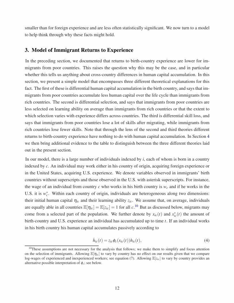
3. Model of Immigrant Returns to Experience

In the preceding section, we documented that returns to birth-country experience are lower for im-

migrants from poor countries. This raises the question why this may be the case, and in particular

whether this tells us anything about cross-country differences in human capital accumulation. In this

section, we present a simple model that encompasses three different theoretical explanations for this

fact. The first of these is differential human capital accumulation in the birth country, and says that im-

migrants from poor countries accumulate less human capital over the life cycle than immigrants from

rich countries. The second is differential selection, and says that immigrants from poor countries are

less selected on learning ability on average than immigrants from rich countries or that the extent to

which selection varies with experience differs across countries. The third is differential skill loss, and

says that immigrants from poor countries lose a lot of skills after migrating, while immigrants from

rich countries lose fewer skills. Note that through the lens of the second and third theories different

returns to birth-country experience have nothing to do with human capital accumulation. In Section 4

we then bring additional evidence to the table to distinguish between the three different theories laid

out in the present section.

In our model, there is a large number of individuals indexed by i, each of whom is born in a country

indexed by c. An individual may work either in his country of origin, acquiring foreign experience or

in the United States, acquiring U.S. experience. We denote variables observed in immigrants’ birth

countries without superscripts and those observed in the U.S. with asterisk superscripts. For instance,

the wage of an individual from country c who works in his birth country is wc and if he works in the

U.S. it is w∗c . Within each country of origin, individuals are heterogeneous along two dimensions:

their initial human capital ηic and their learning ability zic. We assume that, on average, individuals

are equally able in all countries E[ηic] = E[zic] = 1 for all c.10 But as discussed below, migrants may

come from a selected part of the population. We further denote by xic(t) and x∗ic(t) the amount of

birth-country and U.S. experience an individual has accumulated up to time t. If an individual works

in his birth country his human capital accumulates passively according to

hic(t) = zicφc(xic(t))hic(t), (4)

10These assumptions are not necessary for the analysis that follows; we make them to simplify and focus attention

on the selection of immigrants. Allowing E[ηic] to vary by country has no effect on our results given that we compare

log-wages of experienced and inexperienced workers; see equation (7). Allowing E[zic] to vary by country provides an

alternative possible interpretation of φc; see below.

12

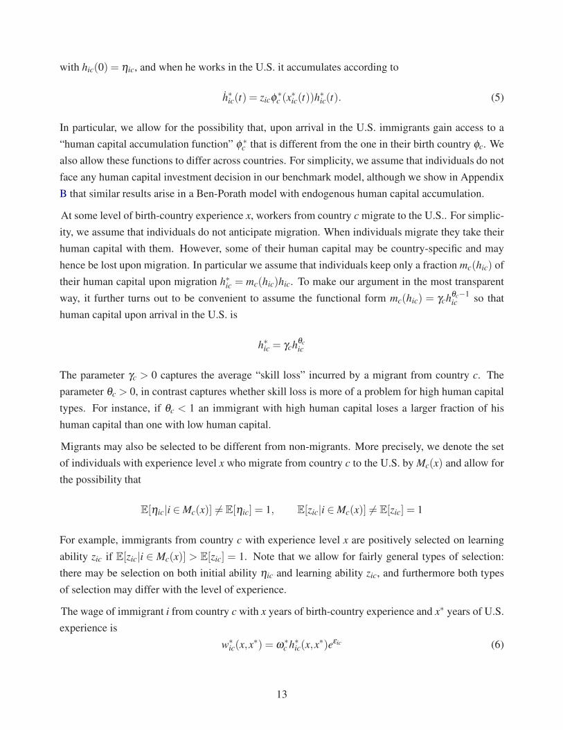
with hic(0) = ηic, and when he works in the U.S. it accumulates according to

h∗ic(t) = zicφ∗c (x

∗ic(t))h

∗ic(t). (5)

In particular, we allow for the possibility that, upon arrival in the U.S. immigrants gain access to a

“human capital accumulation function” φ∗c that is different from the one in their birth country φc. We

also allow these functions to differ across countries. For simplicity, we assume that individuals do not

face any human capital investment decision in our benchmark model, although we show in Appendix

B that similar results arise in a Ben-Porath model with endogenous human capital accumulation.

At some level of birth-country experience x, workers from country c migrate to the U.S.. For simplic-

ity, we assume that individuals do not anticipate migration. When individuals migrate they take their

human capital with them. However, some of their human capital may be country-specific and may

hence be lost upon migration. In particular we assume that individuals keep only a fraction mc(hic) of

their human capital upon migration h∗ic = mc(hic)hic. To make our argument in the most transparent

way, it further turns out to be convenient to assume the functional form mc(hic) = γchθc−1ic so that

human capital upon arrival in the U.S. is

h∗ic = γchθc

ic

The parameter γc > 0 captures the average “skill loss” incurred by a migrant from country c. The

parameter θc > 0, in contrast captures whether skill loss is more of a problem for high human capital

types. For instance, if θc < 1 an immigrant with high human capital loses a larger fraction of his

human capital than one with low human capital.

Migrants may also be selected to be different from non-migrants. More precisely, we denote the set

of individuals with experience level x who migrate from country c to the U.S. by Mc(x) and allow for

the possibility that

E[ηic|i ∈ Mc(x)] 6= E[ηic] = 1, E[zic|i ∈ Mc(x)] 6= E[zic] = 1

For example, immigrants from country c with experience level x are positively selected on learning

ability zic if E[zic|i ∈ Mc(x)] > E[zic] = 1. Note that we allow for fairly general types of selection:

there may be selection on both initial ability ηic and learning ability zic, and furthermore both types

of selection may differ with the level of experience.

The wage of immigrant i from country c with x years of birth-country experience and x∗ years of U.S.

experience is

w∗ic(x,x

∗) = ω∗c h∗ic(x,x

∗)eεic (6)

13

where ω∗c is the skill price earned by immigrants from country c in the U.S. and εic is an error term.

Given our assumptions, the immigrant’s human capital can be solved for in closed form and satisfies11

logh∗ic(x,x∗) = logγc + logηic +θczic

∫ x

0φc(y)dy+ zic

∫ x+x∗

xφ∗

c (y)dy (7)

Combining with (6), the wage of a new immigrant, i.e. one with zero years of U.S. experience x∗ = 0,

is therefore

logw∗ic(x,0) = logω∗

c + logγc + logηic +θczic fc(x)+ εic (8)

where we denote by fc(x) =∫ x

0 φc(y)dy the cumulative returns to foreign experience. The regression

we run using data on new immigrants only is therefore

logw∗ic = αc +Rc(xic)+ εic, Rc(x) = E[logηic|i ∈ Mc(x)]+θcE[zic|i ∈ Mc(x)] fc(x) (9)

The measured return to foreign experience Rc(x) may be low for one of three reasons. First, the true

returns to experience fc(x) may be low. Second, there may be selection. This can either take the

form of experience-dependent selection on initial ability, i.e. E[logηic|i ∈ Mc(x)] decreases with x

or selection on learning ability (both experience-dependent and standard selection are a problem, i.e.

E[zic|i ∈ Mc(x)] is either less than one or decreasing). Third, there may be experience-dependent skill

loss, θc < 1. Estimates from the regression (9) by themselves do not allow us to distinguish between

these three determinants of low measured returns to foreign experience.

In contrast, note that two other potential issues do not show up as low measured returns to foreign

experience: selection on initial ability and skill-loss that are not experience-dependent (i.e. Mc(x) =

Mc with E[logηic|i∈Mc]< 1 and γc < 1). These will simply be picked up the country fixed effects αc.

In the next section, we bring additional evidence to the table to distinguish between the three different

theories: differential human capital accumulation, differential skill loss, and differential selection.

4. Distinguishing Between Theories

In this section we draw on new data to compare the characteristics of immigrants and non-migrants

from a large set of countries. We draw on three basic facts that help us distinguish between the theories

above. First, returns to foreign experience among immigrants are similar to returns to experience

among non-migrants. Second, immigrants from poor countries tend to be more selected on pre-

migration characteristics such as years of schooling. Third, educated immigrants tend to work in

11To see this note that for example (4) can be integrated to yield

loghic(x,x) = logηic + zic

∫ x

0φc(y)dy.

Following similar steps yields (7).

14

high-skilled occupations at a lower frequency than non-migrants, though at a similar rate in rich and

poor countries alike.

4.1. Returns to Experience Among Immigrants and Non-Migrants

We begin by comparing our returns to foreign experience among immigrants to the returns among

non-migrants estimated by Lagakos et al. (2016). We can make these comparisons in the 16 countries

for which we have an estimate of immigrant returns, and for which Lagakos et al. (2016) calculate re-

turns using a representative sample of non-migrants. Since we have followed the sample selection and

variable construction of Lagakos et al. (2016) closely, the comparability of the results is informative

about the extent to which life-cycle wage growth differs between immigrants and non-migrants. We

begin by plotting the estimated returns to 20–24 years of experience against GDP per capita in Figure

6. As one can see from the figure, both estimates show a strong positive relationship with GDP per

capita, with higher returns to experience, on average, in the economies with higher GDP per capita.

Among immigrants, the slope coefficient in a regression of GDP per capita is 29.6 for the immigrants,

with a P-value less than 0.001. Among non-migrants the slope coefficient is 25.2 and the P-value is

less than 0.001.

Figure 7 plots the estimated returns to 20–24 years of experience for immigrants against the same

estimated return for non-migrants. The 45-degree line is also plotted for reference. As one can see,

there is a strong positive relationship between the two sets of estimates; the correlation coefficient

between the two estimates is 0.806 with a P-value of 0.001, although there are some outliers such as

Indonesia and South Korea. Countries like Germany, the UK, and Australia have high returns among

both immigrants and non-migrants, and most of the developing countries have low returns in both

groups.

Perhaps the most striking fact is that these trends do not simply reflect the general influence of being

more developed. To make this point, we first regress both the estimated returns to experience of

immigrants and non-migrants on log real GDP per capita. In Figure 8, we then plot the residuals from

these regressions, which remove the general effect of income. These residuals are also quite strongly

correlated: the correlation coefficient is 0.4760 with a P-value of 0.06. This estimate shows that if a

country’s residents have unusually steep wage profiles for its income level, then its emigrants to the

U.S. are likely to have unusually steep wage profiles too. This provides further evidence in favor of

an explanation that stresses a common factor between immigrants and non-migrants, such as human

capital accumulation. One additional type of evidence favoring the theory that experience human

capital accumulation is higher in the U.S. than in developing countries comes from return migrants.

Reinhold and Thom (2013) find that Mexican immigrants to the United States earn a large premium

on their U.S. experience when returning to Mexico.

The fact that estimated returns to experience from poor countries are low both for immigrants and

15

non-migrants provides one piece of evidence against differential selection as a theory of the immigrant

evidence. If low returns to experience among immigrants were driven solely by negative selection by

immigrants from poor countries, one would expect the returns to experience among non-migrants to

be similar in countries of all income levels. As Figures 6 – 8 show, this is not the case. The broad

similarity between returns to experience among immigrants and non-migrants is also evidence against

differential skill loss as a theory of the immigrant returns. If low returns among immigrants from poor

countries were solely due to skill loss, one would again expect the returns to experience among non-

migrants to be similar in countries of all income levels. This prediction is not borne out in the figures.

Instead, the figures suggest a world where workers in poor countries do not acquire much human

capital while in their birth countries.

4.2. Comparing Other Characteristics of Immigrants and Non-Migrants

Previous work in the immigration literature has considered two additional factors that may affect

returns to experience for immigrants: selection and skill loss. Our main concern is that selection

or skill loss works differently for immigrants from poor and rich countries, and that this differential

selection or skill loss explains why returns to experience vary with GDP per capita. To address each

of these possibilities, we combine evidence from immigrants with data on non-migrants from a large

set of countries for which appropriate data are available. In particular, we use data on education and

occupation from as many countries as possible from nationally representative surveys from IPUMS

(Minnesota Population Center, 2015). This data source is ideal because the creators have devoted

substantial effort to harmonizing variables across countries in a way that is also compatible with our

data on immigrants. To further maximize this benefit, we use a much broader sample in this section,

including any adults with valid responses to the pertinent variables.

We begin by addressing the hypothesis of differential selection. In short, this theory states that im-

migrants from rich countries are more positively selected (or less negatively selected) on ability to

learn than immigrants from poor countries, where ability to learn is an individual trait that affects the

human capital generated per year of potential experience. To test this hypothesis, we consider the av-

erage years of schooling for immigrants and non-migrants. Our underlying assumption is that ability

to learn will be positively correlated with duration of schooling, which allows us to make inferences

about ability selection from data on school selection.

Figure 9 shows the results. The left-hand panel shows that average years of schooling among non-

migrants is strongly correlated with log GDP per capita, with less than five years of schooling on

average in the poorest countries and more than twelve years on average in the richest. In contrast,

the right-hand panel shows that immigrants from countries of all income levels are highly educated

on average, with the majority having roughly twelve years of schooling. These data do not support

the differential selection hypothesis, because immigrants from poorer countries are actually much

16

more positively selected on schooling attainment than are immigrants from richer countries. These

data suggest that some alternative force, such as differences in education quality, or the type of work

performed, or the incentives to invest in human capital accumulation on the job, are more likely

explanations of flat life-cycle wage profiles for immigrants from poor countries.

These findings are consistent with most evidence from previous studies. Grogger and Hanson (2011)

show that, across a wide set of countries, the share of college educated workers among immigrants is

substantially higher than the same share among all individuals. They argue that this implies positive

selection among immigrants in general. Ehrlich and Kim (2015) shows a similar result for migrants

to a wide range of countries. Hendricks and Schoellman (2016) show that immigrants to the U.S. are

strongly selected on a large range of characteristics, including pre-migration wages, occupation, and

education, and that immigrants from poorer countries are more selected on these dimensions. There

are perhaps some key exceptions, mostly the countries near the U.S. where unauthorized immigration

plays a large role. For example, Moraga (2011) suggests that Mexican immigrants may be negatively

selected. Fortunately, as we documented above our results are robust to focusing on countries with

low rates of unauthorized immigration.

We now turn to the hypothesis of differential skill loss. Briefly, this theory says that immigrants from

rich countries can transfer more of their experience human capital to the U.S. than can immigrants

from poor countries. To test this hypothesis, we compare rates of skill loss for immigrants and non-

migrants. We restrict the sample to workers and define them as experiencing skill loss if they have a

college education (our notion of “skilled”) but work in a low-skilled occupation.12 For each country,

we calculate the fraction of all college-educated immigrants and non-migrants that work in high-

skilled occupations.

Figure 10 plots the results. The left-hand panel shows that among non-migrants, a high fraction

of college-educated workers are in high-skill jobs in countries of all income levels. The fraction

is increasing in GDP per capita, meaning that college-educated workers in rich countries tend to

work at high-skilled jobs with higher frequency. The right-hand panel shows that a large fraction of

college-educated immigrants are employed at high-skilled jobs as well, and that the relationship is

also increasing in the GDP per capita of the birth country. It is clear that immigrants are less likely

to work at high skilled jobs than non-migrants in countries of any income level. This is consistent

with the presence of skill loss. However, the slopes for immigrants and non-migrants appear similar,

suggesting that skill loss is present to a similar degree in countries of all income levels. This is

evidence against the possibility that our findings are explained by differential skill loss.

12IPUMS has standardized occupation codes across all our data sources. We define high skilled to be “professionals,”

“technicians and associate professionals,” and “legislators, senior officials and managers,” and low skilled to be “clerks,

service workers and shop and market sales,” “skilled agricultural and fishery workers,” “crafts and related trades workers,”

“plant and machine operators and assemblers” and “elementary occupations.” We omit individuals in the armed forces or

other unspecified or unreported occupations.

17

We also investigate a more subtle form of differential selection or skill loss that operates through an

association with experience. The idea here is that immigrants with more experience may be selected

differently than those with less experience, and that the difference in how selected they are may be

correlated with GDP per capita; a similar story works for skill loss. To test this, we compared selection

or skill loss (as defined above) between two discrete groups, those with low and high experience

(defined as less than ten and ten or more years of experience). The results are shown in Figures 10

and 11. In each figure a comparison of the upper left and bottom left figures shows the unsurprising

result that low and high experience non-migrants have similar patterns of educational attainment and

skill loss. More importantly, a comparison of the upper right and bottom right figures shows that the

extent of selection on education and skill loss is remarkably similar for less and more experienced

immigrants. In particular, there is little evidence that the relationship between educational selection

or skill loss and GDP per capita varies between less and more experienced workers.

The results on selection and skill loss, when combined with the fact that returns to experience patterns

are strongly correlated with the same patterns for non-migrants, suggest that cross-country differences

in human capital accumulation are the most plausible interpretation of the data.

5. Development Accounting

In this section we use development accounting to quantify the economic importance of the empirical

results shown in Section 2. To keep our findings as comparable as possible to the previous literature,

we follow the accounting approach of Klenow and Rodrıguez-Clare (1997), Hall and Jones (1999)

and in particular Caselli (2005).

The accounting procedure uses a Cobb-Douglas aggregate production function Yc = Kαc (AcHc)

1−α ,

where Yc is GDP per worker of country c, Kc is physical capital per worker and Hc is human capital

per worker. The capital share is assumed to equal one-third. As in Caselli (2005), we calculate the

measure

success1 =var (logYKH,c)

var (logYc)

where YKH,c = Kαc H1−α

c is the component of output due to factors of production. Values of success1

close to one suggest that cross-country differences in capital stocks account for nearly all of measured

income differences. Values close to zero imply that capital stocks account for none of income dif-

ferences. One limitation of the measure success1 is that measurement error in YKH,c could increase

success1, while clearly this does not imply a greater importance of capital stocks. Thus, to comple-

ment the successes metric, we also report the slope of a regression of logYKH,c on logYc.

To highlight the difference between our findings and those of the previous literature, we use the

same physical capital estimates as Caselli (2005), and assume that all individuals in a given country

18

have the same levels of schooling and experience sc and xc (also taking these averages from Caselli

(2005)). Our measure of the stock of human capital differs only in the assumed life-cycle profile of

labor market productivity. Instead of assuming that this profile is common across countries, we use

estimated profiles similar to those from Section 2, but utilizing the broadest possible sample, including

women, part-time workers, and public employees. Our logic is that development accounting results

should reflect the full labor force, but as we showed in Table 2, the estimated results are similar with

or without these groups. Thus, we find similar development accounting results if we use instead the

baseline results of Section 2.

We consider two assumptions on the life-cycle labor market productivity profile, corresponding to

whether we view human capital as the result of passive investment (simple learning-by-doing, as in

Section 3) or active accumulation (Ben-Porath, as in Appendix B). These two models differ slightly in

their interpretation of life-cycle increases in wages. The former attributes all of this increase to rising

human capital over the life cycle. By contrast, the latter attributes some of this increase to an increase

in time spent producing and a decrease in time spent investing at work over the life cycle.

Both of these formulations allow us to express the human capital of a worker with years of schooling

s and experience x in country c as

hc(s,x) = exp(gc(s)+ fc(x)).

The functions gc and fc measure the human capital returns to schooling and experience.13 The ag-

gregate human capital stock of country c is then simply defined as the human capital of an individual

with the average years of schooling and experience, Hc = hc(sc, xc). As discussed above, in the case

of active accumulation of human capital the return to foreign experience measured in the U.S. R∗c(x,0)

captures both the increase in human capital over the life cycle fc(x) and a term due to changes in the

amount of time allocated towards human capital accumulation:

R∗c(x,0) = fc(x)+ log

(

1− ℓ∗c(x)

1− ℓc(0)

)

.

See Appendix B for details of the derivation.

We conduct two alternative accounting exercises, which provide an upper bound and lower bound

on the importance of human capital in development accounting implied by our empirical results. We

begin with the upper bound, which assumes that the investment time allocation, ℓc(x), is constant

across experience levels for each country. This assumption allows us to measure human capital ac-

cumulation directly from the experience-wage profiles as fc(x) = Rc(x,0). Given that most countries

13The connection to the model in the Appendix is a bit more subtle in this respect. Experience human capi-

tal accumulates according to hc = φc(ℓc)hc − δhc and hence its logarithm at experience level x can be written as

loghc(x) =∫ x

0 (φc(ℓc(x))− δ )dx.

19

have roughly 17 years of experience on average, we use the estimated returns to 15–19 years of expe-

rience (Caselli, 2005). From the perspective of a passive investment model this is the correct measure

of human capital because the investment time allocation is constant at 0. From the perspective of a

Ben-Porath model this overstates the importance of experience human capital because time devoted to

human capital investment is decreasing over the life cycle in all countries but more so in richer coun-

tries, implying that log(

1−ℓ∗c(x)1−ℓc(0)

)

is positive and increasing in GDP per capita. By abstracting from

this we have overstated cross-country human capital differences from the perspective of a Ben-Porath

model.

We plot our estimated human capital stocks against GDP per capita in Figure 13. This figure plots the

human capital stocks implied by our upper bound, and the slope from a regression of human capital

stocks measured only using schooling on log GDP per capita. As the figure shows, our estimated

human capital stocks are substantially larger in rich countries than poor countries once experience is

included.

The accounting under this upper bound is presented in the top panel of Table 3. The first column

presents our measures of success1. When only schooling is taken into consideration, success1 is

0.44, meaning that human and physical capital account for just under one half of income differences.

When only experience is considered, success1 is similar, at 0.48. When they are both considered,

success1 rises to 0.74, meaning that now almost three-fourths of income differences are accounted

for by measured capital stocks. The second column shows that the correlation of measured capital

stocks and GDP per capita rises substantially as well. With just schooling or just experience, the

slope coefficient from a regression of log(YKH) on log(GDP) is 0.63 and 0.65. With both schooling

and experience used to compute human capital stocks, the slope coefficient rises to 0.81. Thus, under

this upper bound at least, the importance of human capital increases substantially when we include

experience human capital estimated using immigrant returns to experience.

We turn now to our second accounting exercise, which provides a lower bound on the importance

of human capital implied by our empirical findings. The challenge to providing a lower bound is

bounding the endogenous changes in life-cycle human capital investment. In Appendix B, we show

that in a simple Ben-Porath model the time devoted to human capital investment for immigrants

depends only on the remaining working life and the exogenous efficiency of their human capital

accumulation in the U.S. (T − t and B∗c in the notation of Appendix B; see Lemma 1). We show there

that a useful intermediate step is to study the difference between the returns to xc = 15−19 years of

foreign experience and x∗c = 15−19 years of U.S. for immigrants from c. This is useful because both

groups of immigrants face the same remaining working life and the same efficiency of human capital

investment going forward; hence, they are predicted to invest the same fraction of their time in human

capital accumulation. By taking the difference between the two we can focus on the difference in

human capital stocks.

20

While the level of the difference in human capital stocks is not useful, its variance and correlation with

GDP per capita are. To see why, note that returns to U.S. experience are weakly increasing in GDP per

capita, which implies that human capital stocks are weakly increasing in GDP per capita. In the simple

case where the U.S.-acquired human capital stock is constant, we are subtracting a constant from all

countries. Hence, the variance and correlation would capture exactly the variance and correlation

of foreign human capital stocks and the lower bound would be exact. If the U.S.-acquired human

capital stock is strictly increasing in GDP per capita then we are biasing downward the variance and

correlation, implying that we have found a lower bound on the importance of foreign-acquired human

capital stocks.

The accounting under this lower bound is presented in the bottom panel of Table 3. This time, when

human capital from both schooling and experience are taken into consideration, success1 is 0.66, up

from 0.44 when only schooling is considered. The slope coefficient from a regression of log(YKH)

on log(GDP) is 0.76, up from 0.63 when only schooling is considered as human capital. It is also

important to note that our bounding exercise produces a relatively tight range on the importance of

human capital for development accounting: between 0.66 and 0.74 by the first criteria and between

0.76 and 0.81 by the second criteria. We conclude that the importance of human capital increases

greatly when experience is included, regardless of whether life-cycle wage growth is driven by passive

or active investment in human capital accumulation.

6. Conclusion

This paper seeks to understand whether workers in richer countries acquire more human capital over

the life cycle than workers in poor countries. The answer has first-order implications for the literature

that attempts to account for cross-country income differences using measured stocks of human and

physical capital. Previous studies have concluded that cross-country differences in life-cycle human

capital accumulation are negligible, and that the overall importance of human capital in accounting

for income differences is modest (Klenow and Rodrıguez-Clare, 1997; Bils and Klenow, 2000, 1998;

Caselli, 2005). Yet more recent work claims that human capital plays a much more central role

(Manuelli and Seshadri, 2015; Lagakos et al., 2016).

To address this question, this paper draws on evidence from U.S. immigrants, who come from coun-

tries of all income levels but work in a common labor market. We document that immigrants from

richer countries tend to have higher returns to potential experience than immigrants coming from poor

countries. We argue that the most likely explanation of this fact is that workers in rich countries sim-

ply acquire more human capital before migrating. Another logical possibility is that immigrants from

rich countries are just better selected on learning ability than immigrants from the developing world.

Yet this contrasts with the observation that immigrants from poor countries tend to be much better ed-

21

ucated than their counterparts that did not migrate, whereas immigrants from richer countries are only

modestly more educated than non-migrants from the same countries. Yet another possibility is that

immigrants from poor countries disproportionately lose skills after migrating. But this contrasts with

evidence on the occupations of immigrants compared to non-migrants, which suggest similar skill

loss across countries. Finally, the fact that returns to experience are similar between immigrants and

non-migrants, in most countries, is most consistent with a model in which workers in poor countries

simply accumulate less human capital during their working years.

Why are our findings relevant for macroeconomics? A large literature on development accounting

has concluded that human capital accounts for at best a modest fraction of living standard differences

across countries. This literature has concluded that including differences in life-cycle human capital

accumulation (i.e. human capital from experience) does not change the accounting. In contrast, our

findings point to a very different conclusion, which is that life-cycle human capital differences are

large. Our development accounting, based on our evidence from U.S. immigrants, suggests a much

larger role for human capital in accounting for cross-country income differences.

A natural but challenging next step is to explain why life-cycle human capital accumulation tends

to be lower in poor countries than rich countries. One possible explanation is that the quantity and

type of schooling results in less “learning how to learn” among individuals who attend school in

poor countries. We have found support for this hypothesis by documenting that the returns to U.S.

experience among foreign-educated workers are lower than the returns to U.S. experience for natives.

At the same time, we have also documented that the returns to U.S. experience among U.S.-educated

workers are very similar to those of natives. Combined, these two facts suggest a complementarity

between both quantity and type of education and subsequent human capital accumulation that may be

worth exploring further in the future.

22

References

Bils, M. and P. J. Klenow (1998). Does schooling cause growth or the other way around? NBER

Working Papers 6393, National Bureau of Economic Research.

Bils, M. and P. J. Klenow (2000). Does schooling cause growth? American Economic Review 90(5),

1160–83.

Borjas, G. J. (1985). Assimilation, changes in cohort quality and the earnings of immigrants. Journal

of Labor Economics 3(4), 463–489.

Caron, J., T. Fally, and J. R. Markusen (2014). International trade puzzles: A solution linking produc-

tion and preferences. Quarterly Journal of Economics 129(3), 1501–1552.

Caselli, F. (2005). Accounting for cross-country income differences. In P. Aghion and S. Durlauf.

(Eds.), Handbook of Economic Growth, 679-741. Elsevier.

Chiswick, B. R. (1978). The effect of Americanization on the earnings of foreign-born men. Journal

of Political Economy 86(5), 897–921.

Coulombe, S., G. Grenier, and S. Nadeau (2014). Quality of work experience and economic develop-

ment: Estimates using Canadian data. Journal of Human Capital 8(3), 199–234.

Ehrlich, I. and J. Kim (2015). Immigration, human capital formation, and endogenous economic

growth. Journal of Human Capital 9(4), 518–563.

Erosa, A., T. Koreshkova, and D. Restuccia (2010). How important is human capital? A quantitative

theory assessment of world income inequality. Review of Economic Studies 77(4), 1421–49.

Friedberg, R. M. (1992). The labor market assimilation of immigrations in the United States: The

role of age at arrival. Unpublished Manuscript, Brown University.

Grogger, J. and G. H. Hanson (2011). Income maximization and the selection and sorting of interna-

tional migrants. Journal of Development Economics 95(1), 42–57.

Hall, R. E. and C. I. Jones (1999). Why do some countries produce so much more output per worker

than others? Quarterly Journal of Economics 114(1), 83–116.

Hanushek, E. A. and D. D. Kimko (2000, December). Schooling, labor-force quality, and the growth

of nations. American Economic Review 90(5), 1184–1208.

Hendricks, L. (2002). How important is human capital for development? Evidence from immigrant

earnings. American Economic Review 92(1), 198–219.

23

Hendricks, L. and T. Schoellman (2016). Human capital and development accounting: New evidence

from wage gains at migration. mimeo, University of North Carolina - Chapel Hill.

Hsieh, C.-T. and P. J. Klenow (2010). Development accounting. American Economic Journal:

Macroeconomics 2(1), 207–23.

Klenow, P. J. and A. Rodrıguez-Clare (1997). The neoclassical revival in growth economics: Has it

gone too far? In B. S. Bernanke and J. Rotemberg (Eds.), NBER Macroeconomics Annual 1997.

Cambridge: MIT Press.

Lagakos, D., B. Moll, T. Porzio, N. Qian, and T. Schoellman (2016). Life-cycle wage growth across

countries. Unpublished Manuscript, Princeton University.

Lemieux, T. (2006). The “Mincer Equation” thirty years after Schooling, Experience, and Earnings.

In S. Grossbard (Ed.), Jacob Mincer: A Pioneer of Modern Labor Economics, Chapter 11, pp.

127–145. Spring.

Lewis, J. B. and D. A. Linzer (2005). Estimating regression models in which the dependent variable

is based on estimates. Political Analysis 13(4), 345–364.

Manuelli, R. E. and A. Seshadri (2015). Human capital and the wealth of nations. American Economic

Review 104(9), 2736–2762.

Mincer, J. (1974). Schooling, Experience and Earnings. New York: Columbia University Press.

Minnesota Population Center (2015). Integrated public use microdata series-international: Version

6.4. [Machine-readable database]. Minneapolis: University of Minnesota.

Moraga, J. F.-H. (2011). New evidence on emigrant selection. The Review of Economics and Statis-

tics 93(1), 72–96.

Office of Policy and Planning, U.S. Immigration and Naturalization Service (2003, January). Esti-

mates of the unauthorized immigrant population residing in the United States: 1990 to 2000.

Psacharopoulos, G. (1994). Returns to investment in education: A global update. World Develop-

ment 22(9), 1325–43.

Reinhold, S. and K. Thom (2013). Migration experience and earnings in the Mexican labor market.

Journal of Human Resources 48(3), 768–820.

Ruggles, S., K. Genadek, J. Grover, and M. Sobek (2015). Integrated public use microdata series:

Version 6.0. [Machine-readable database]. Minneapolis: University of Minnesota.

24

Schoellman, T. (2012). Education quality and development accounting. Review of Economic Stud-

ies 79(1), 388–417.

World Bank (2015). World Development Indicators.

25

Table 1: Summary Statistics for Sample and Select Countries

Wage U.S. Exp. For. Exp. Schooling English Number

Summary Statistics: All Immigrants

Mean 0.96 13.0 7.6 11.1 3.0 771,952

S.D. 1.00 8.8 7.4 4.7 1.2

Sample Means: Select Countries

Mexico 0.63 13.3 5.8 8.5 2.4 280,955

India 1.82 10.0 7.0 16.3 3.8 38,208

Philippines 1.14 14.4 9.8 14.4 3.6 29,905

El Salvador 0.67 13.7 6.1 8.6 2.6 26,476

China 1.26 12.7 9.8 14.1 2.8 24,075

Vietnam 0.90 16.2 9.2 11.3 2.8 20,058

Guatemala 0.59 10.7 6.1 8.0 2.4 18,465

United Kingdom 2.40 12.4 10.2 15.4 4.9 18,231

Cuba 0.78 11.7 12.5 12.4 2.6 16,266

Canada 2.16 12.3 9.9 15.1 4.7 15,567

Note: table gives summary statistics for the baseline sample for all immigrants (first row) and the ten countries

with the most immigrants in the baseline sample. Wage is hourly wage, taken relative to natives in the given

year and averaged across years. (Potential) experience and schooling are measured in years. English is the

respondent’s self-rated English ability, ranking from 1 to 5 where 1 corresponds to “Does not speak English”

and 5 corresponds to “Speaks only English”. Number is the sample size. All figures are weighted by within-

sample weights and summed across years.

26

Table 2: Returns to Experience and GDP per capita: Robustness of Results

Schooling: Foreign Foreign U.S.

Experience: Foreign U.S. U.S.

Sample:

Baseline 20.0*** 5.6* 7.0*

15–19 Years Experience 15.2*** 3.3 1.5

Average Height of Profile 16.4*** 5.5** 6.1

Discounted Average Height of Profile 8.4*** 2.6** 3.3**

Weighted by Sample Size 23.2*** 3.7 1.9

Weighted by Population 31.3*** 6.0 -0.3

Include Women 20.2*** 3.6 2.6

Include Some Part-Time 20.5*** 5.3* 7.1*

Include All Part-Time 23.7*** 7.8*** 3.9

Include Public Sector 21.4*** 6.3** 10.9***

Year 2000+ 21.9*** 6.3* 7.0*

Country-Specific School Start Date 18.7*** 1.9 N/A

Experience at 16 20.9*** 3.3 1.5

Ages 18–65 19.9*** 5.6* 10.3

Ages 22–55 23.1*** 6.1* 7.4**

≥College Graduate 38.6*** 5.4 10.2*

≤H.S. Graduate 13.8*** 5.0* N/A

Variable Return to Schooling 20.9*** 0.6 N/A

Manufacturing 15.7*** 5.4 N/A

Service Industry 23.2*** 11.5*** 7.0

Excellent English 26.4*** 6.6* 6.2*

English-Speaking Country 14.3*** 2.6 N/A

No Ethnic Enclaves 22.5*** 6.2* 7.3*

Fewer Unauthorized Immigrants 20.9*** 6.3** 5.3

Note: table reports estimates from a second-stage regression of the estimated height of experience profiles on log Real

GDP p.c. Each row corresponds to a sample for the first-stage regression, specification for the first-stage regression, or

measure of the height of experience profiles; see the text for details. The columns correspond to the estimated value of

foreign experience, U.S. experience for foreign educated immigrants, and U.S. experience for immigrants with some

U.S. education. ***, **, and * denote results that are significant at the 1 percent, 5 percent, and 10 percent. N/A

denotes a check that is not available because it is logically inconsistent (country-specific school start date) or there are

too few countries in the sample (less than 15).

27

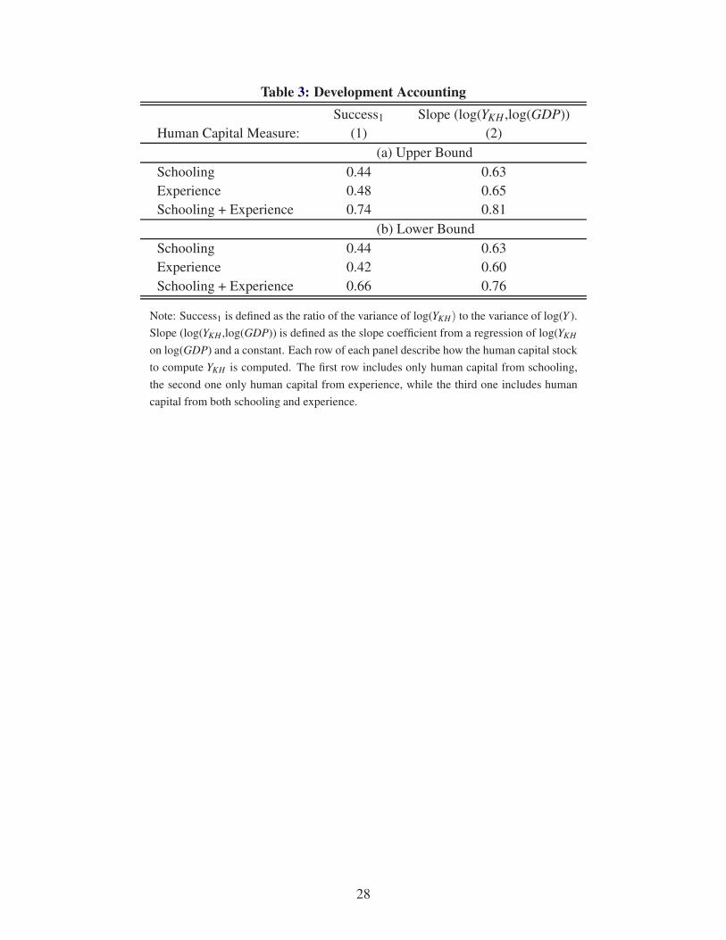
Table 3: Development Accounting

Success1 Slope (log(YKH ,log(GDP))

Human Capital Measure: (1) (2)

(a) Upper Bound

Schooling 0.44 0.63

Experience 0.48 0.65

Schooling + Experience 0.74 0.81

(b) Lower Bound

Schooling 0.44 0.63

Experience 0.42 0.60

Schooling + Experience 0.66 0.76

Note: Success1 is defined as the ratio of the variance of log(YKH) to the variance of log(Y ).

Slope (log(YKH ,log(GDP)) is defined as the slope coefficient from a regression of log(YKH

on log(GDP) and a constant. Each row of each panel describe how the human capital stock

to compute YKH is computed. The first row includes only human capital from schooling,

the second one only human capital from experience, while the third one includes human

capital from both schooling and experience.

28

0

50

100

150

200

250P

erc

en

t W

ag

e I

ncre

ase

Re

lative

to

0−

4 Y

ea

rs

0 10 20 30Years of Foreign Experience

Canada United Kingdom

Guatemala Mexico

Figure 1: Returns to Foreign Experience Among New Immigrants, Select Countries. Shaded Regions

are the 95% Heteroskedasticity Robust Confidence Intervals.

29

0

50

100

150

Wa

ge

s a

t 2

0−

24

Re

lative

to

0−

4 Y

ea

rs E

xp

erie

nce

1000 2500 5000 10000 20000 40000Real GDP p.c., 2010, Log Scale

Figure 2: Returns to Foreign Experience Among New Immigrants by Real GDP p.c. of Birth Country.

Shaded Region is the 95% Heteroskedasticity Robust Confidence Intervals.

30

0

50

100

150W

ag

es a

t 2

0−

24

Re

lative

to

0−

4 Y

ea

rs E

xp

erie

nce

1000 2500 5000 10000 20000 40000Real GDP p.c., 2010, Log Scale

Foreign Experience U.S. Experience

Figure 3: Returns to Foreign and U.S. Experience by Real GDP p.c. of Birth Country. Shaded Regions

are the 95% Heteroskedasticity Robust Confidence Intervals.

31

0

50

100

150W

ag

es a

t 2

0−

24

Re

lative

to

0−

4 Y

ea

rs E

xp

erie

nce

1000 2500 5000 10000 20000 40000Real GDP p.c., 2010, Log Scale

High School or Less College or More

Figure 4: Returns to U.S. Experience by Education Level by Real GDP p.c. of Birth Country. Shaded

Regions are the 95% Heteroskedasticity Robust Confidence Intervals.

32

0

50

100

150W

ag

es a

t 2

0−

24

Re

lative

to

0−

4 Y

ea

rs E

xp

erie

nce

1000 2500 5000 10000 20000 40000Real GDP p.c., 2010, Log Scale

Foreign School U.S. School

Figure 5: Returns to U.S. Experience by Education Location by Real GDP p.c. of Birth Country.

Shaded Regions are the 95% Heteroskedasticity Robust Confidence Intervals.

33

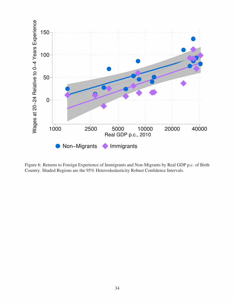
0

50

100

150W

ag

es a

t 2

0−

24

Re

lative

to

0−

4 Y

ea

rs E

xp

erie

nce

1000 2500 5000 10000 20000 40000Real GDP p.c., 2010

Non−Migrants Immigrants

Figure 6: Returns to Foreign Experience of Immigrants and Non-Migrants by Real GDP p.c. of Birth

Country. Shaded Regions are the 95% Heteroskedasticity Robust Confidence Intervals.

34

0

50

100

150Im

mig

ran

ts

0 50 100 150Non−Migrants

Figure 7: Returns to Foreign Experience, Immigrants vs Non-migrants

35

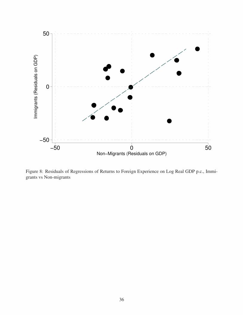
−50

0

50Im

mig

ran

ts (

Re

sid

ua

ls o

n G

DP

)

−50 0 50Non−Migrants (Residuals on GDP)

Figure 8: Residuals of Regressions of Returns to Foreign Experience on Log Real GDP p.c., Immi-

grants vs Non-migrants

36

0

5

10

15A

vera

ge S

choolin

g Y

ears

1000 2500 5000 10000 20000 40000

Real GDP p.c., 2010

Non−Migrants

0

5

10

15

Avera

ge S

choolin

g Y

ears

1000 2500 5000 10000 20000 40000

Real GDP p.c., 2010

Immigrants

Figure 9: Years of Schooling Completed Among Immigrants and Non-migrants

37

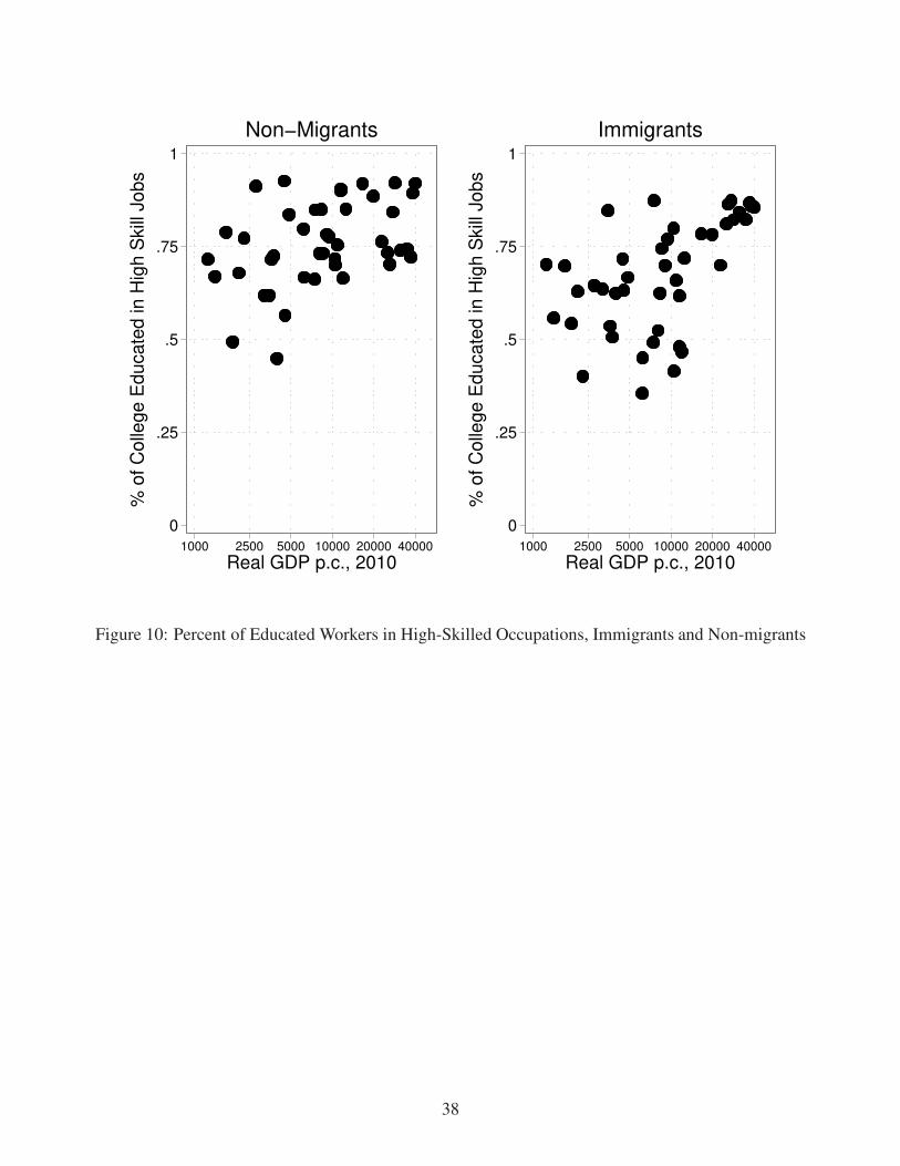
0

.25

.5

.75

1%

of C

olle

ge E

ducate

d in H

igh S

kill

Jobs

1000 2500 5000 10000 20000 40000

Real GDP p.c., 2010

Non−Migrants

0

.25

.5

.75

1

% o

f C

olle

ge E

ducate

d in H

igh S

kill

Jobs

1000 2500 5000 10000 20000 40000

Real GDP p.c., 2010

Immigrants

Figure 10: Percent of Educated Workers in High-Skilled Occupations, Immigrants and Non-migrants

38

0

5

10

15A

vera

ge S

choolin

g Y

ears

1000 2500 5000 10000 20000 40000Real GDP p.c., 2010

Non−Migrants − High Experience

0

5

10

15

Avera

ge S

choolin

g Y

ears

1000 2500 5000 10000 20000 40000

Real GDP p.c., 2010

Immigrants − High Experience

0

5

10

15

Avera

ge S

choolin

g Y

ears

1000 2500 5000 10000 20000 40000Real GDP p.c., 2010

Non−Migrants − Low Experience

0

5

10

15

Avera

ge S

choolin

g Y

ears

1000 2500 5000 10000 20000 40000Real GDP p.c., 2010

Immigrants − Low Experience

Figure 11: Years of Schooling Completed Among Immigrants and Non-migrants by Foreign Experi-

ence Level

39

0

.25

.5

.75

1%

of

Co

lleg

e E

du

ca

ted

in

Hig

h S

kill

Jo

bs

1000 2500 5000 10000 20000 40000Real GDP p.c., 2010

Non−Migrants − High Experience

0

.25

.5

.75

1

% o

f C

olle

ge

Ed

uca

ted

in

Hig

h S

kill

Jo

bs

1000 2500 5000 10000 20000 40000Real GDP p.c., 2010

Immigrants − High Experience

0

.25

.5

.75

1

% o

f C

olle

ge

Ed

uca

ted

in

Hig

h S

kill

Jo

bs

1000 2500 5000 10000 20000 40000Real GDP p.c., 2010

Non−Migrants − Low Experience

0

.25

.5

.75

1

% o

f C

olle

ge

Ed

uca

ted

in

Hig

h S

kill

Jo

bs

1000 2500 5000 10000 20000 40000Real GDP p.c., 2010

Immigrants − Low Experience

Figure 12: Percent of Educated Workers in High-Skilled Occupations, Immigrants and Non-migrants

by Foreign Experience Level

40

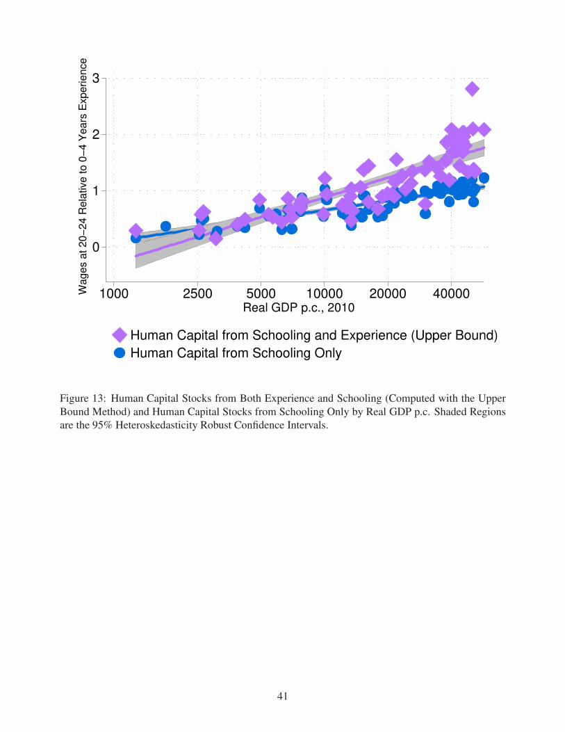
0

1

2

3W

ag

es a

t 2

0−

24

Re

lative

to

0−

4 Y

ea

rs E

xp

erie

nce

1000 2500 5000 10000 20000 40000Real GDP p.c., 2010

Human Capital from Schooling and Experience (Upper Bound)

Human Capital from Schooling Only

Figure 13: Human Capital Stocks from Both Experience and Schooling (Computed with the Upper

Bound Method) and Human Capital Stocks from Schooling Only by Real GDP p.c. Shaded Regions

are the 95% Heteroskedasticity Robust Confidence Intervals.

41

Appendix

A. Estimating Returns to Experience Among Immigrants

The identification issues are mostly clearly explained when we assume that experience, schooling,

and year all enter the regression equation linearly. Given these assumptions the Mincerian regression

equation for natives is then:

log(wN) = β NXN +φ NEN +ωNY N +µNSN + εN (10)

where Greek variables denote the coefficients and ε is the error term. The superscript N is used to

denote natives.

Our primary goal is to study the determinants of immigrants’ earnings. Similar to Chiswick (1978)

and Schoellman (2012), we want to allow the return to foreign-acquired schooling to differ from

U.S.-acquired schooling. We also want to distinguish between the return to foreign (birth country)

and domestic (U.S.) experience for immigrants FE and DE. We will also allow the return to domestic

experience to be different for immigrants and natives.

However, a by-now large literature has proposed alternative possible factors that may matter for the

determinants of immigrants’ earnings, and raised some identification issues that need to be addressed.

Borjas (1985) suggested allowing for year of immigration cohort effects, C, to capture the idea that

immigrants who enter in different years may be drawn from different parts of the income or talent

distribution in their birth country. Friedberg (1992) suggested allowing for an effect of age at arrival,

AA. She hypothesizes that older immigrants will be more invested in their birth country and less able

to adapt to the U.S. Finally, some authors have suggested allowing a role for years in the U.S. YUS

to capture the assimilation of immigrants. Combining all of these potential factors would suggest a

Mincerian regression equation for immigrants:

log(wI) = β IX I +φ I1FEI +φ I

2DEI +ω IY I +µ ISI +α IAAI + γ ICI +δ IYUSI + ε I (11)

where Greek variables denote again coefficients and the superscript I denotes immigrants. Note that

we have allowed the returns to common characteristics (such as S and X ) to vary between natives and

immigrants.

A well-known problem in the literature is that a number of the terms on the right-hand side of equation

(11) are linearly related to one another, in which case it is not possible to identify the corresponding

coefficients. A useful way to express these dependencies is to show that seven of the right-hand side

variables are actually constructed using linear combinations of four survey questions: age, years of

schooling, dataset year, and year of immigration Y II. Years of schooling and dataset year enter the

42

regression equation directly; five other variables in that equation are linear combinations of these four

survey questions:

1. FEI = AI −SI −6− (Y I −Y II)

2. DEI =Y I −Y II

3. AAI = AI − (Y I −Y II)

4. CI =Y II

5. YUSI =Y I −Y II

Equation (11) thus includes seven variables that are linear combinations of four survey questions.

Three assumptions or restrictions are necessary to make estimation feasible.

Our first restriction comes from pooling immigrants and natives into a single regression and restricting

ωN = ω I . The assumption here is that time effects capture aggregate economic conditions such as

recessions or inflation that affect immigrants and natives equally. In this case the time effects can be

estimated for the natives and imposed on the immigrants, reducing the number of equations by one.

The remaining two restrictions are almost definitional in nature. First, note that U.S. experience and

years in U.S. are in fact defined in the same manner. In this case it is impossible to identify separately

the effect of U.S. potential experience from any other, more general effects of spending time in the

U.S., including social assimilation. Hence, we can include only one of these two regressors. In

general, it is not clear whether the resulting estimated coefficient captures the effect of U.S. experience

or of other factors related to years since migration. The second restriction arises from the fact that

foreign potential experience and age at arrival are almost identical: they differ only by the expected

age at graduation, SI + 6. Once again, the implication is that it is difficult to distinguish between

the effects of foreign experience and a more general effect for age at arrival due to, say, adaptability.

However, given that our estimated experience effects for immigrants look strikingly similar to those

estimated in Lagakos et al. (2016) for non-migrants, we believe that our results support assigning a

dominant role to experience human capital.

B. Ben-Porath Model of Human Capital Accumulation

In this Appendix we extend the simple learning-by-doing model of Section 3 to feature endogenous

human capital accumulation. That is, we show that essentially the same insights about differences

in experience-wage profiles for immigrants continue to go through in a Ben-Porath model of human

capital accumulation. We also show how we derive the upper and lower bounds on human capital

accumulation used in Section 5.

43

B.1. Setup

We model the human capital accumulation decision of an individual from country c who may work

either in his country of origin, acquiring foreign experience or in the United States, acquiring U.S.

experience. We denote variables observed in the U.S. with asterisk superscripts, and those observed

abroad without superscripts. For instance, the wage of an individual from country c who works in his

country of origin is wc(t) and if he works in the U.S. it is w∗c(t). Individuals devote a fraction ℓc(t)

of their time to human capital accumulation. If they work in their birth country their human capital

accumulates according to

hc = φc(ℓc)hc −δhc,

and when they are in the U.S. it accumulates according to

hc = φ∗c (ℓc)hc −δhc,

where δ ≥ 0 is the depreciation rate of human capital. We assume that φc(ℓ)=Bcℓσ and φ∗

c (ℓ)=B∗cℓ

σ ,

with σ < 1. The parameters Bc and B∗c determine how quickly human capital accumulates for a given

amount of time devoted to human capital accumulation. Bc may vary across countries and may be

different from B∗c , capturing the idea that countries differ in the quality of their “learning environment.”

We also allow the “learning environment” in the U.S. B∗c to vary across countries so that it matters

where an individual is born, even after migration to the U.S.

The wage in an individual’s home country is wc(t) = ωc(1− ℓc(t))hc(t) and analogously for the U.S.

wage. At some level of home-country experience x, workers from country c migrate to the U.S..

For simplicity, we assume that individuals do not anticipate migration so that their human capital

accumulation decision before migration depends only on the environment in their birth country.14

Finally, we assume that when workers migrate, they take with them their entire human capital stock

so that hc(x∗) = h∗c(x

∗).

As in the simple learning-by-doing model in Section 3, one can extend the model to feature individual-

specific heterogeneity in the parameters Bc and B∗c so as to explore the issue of selection of migrants

with different learning abilities. Similarly, can also extend the model to feature “skill loss” upon

migration. All the insights discussed there would go through.

14This assumption can be relaxed at the expense of some extra notation.

44

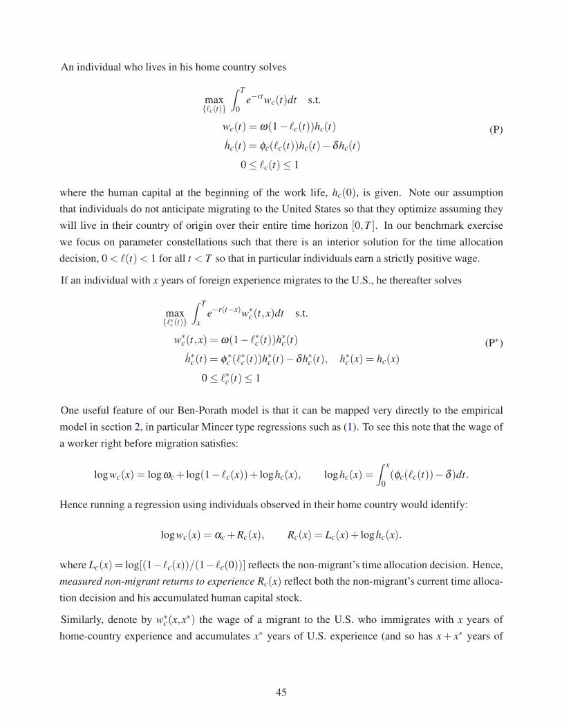
An individual who lives in his home country solves

max{ℓc(t)}

∫ T

0e−rtwc(t)dt s.t.

wc(t) = ω(1− ℓc(t))hc(t)

hc(t) = φc(ℓc(t))hc(t)−δhc(t)

0 ≤ ℓc(t)≤ 1

(P)

where the human capital at the beginning of the work life, hc(0), is given. Note our assumption

that individuals do not anticipate migrating to the United States so that they optimize assuming they

will live in their country of origin over their entire time horizon [0,T ]. In our benchmark exercise

we focus on parameter constellations such that there is an interior solution for the time allocation

decision, 0 < ℓ(t)< 1 for all t < T so that in particular individuals earn a strictly positive wage.

If an individual with x years of foreign experience migrates to the U.S., he thereafter solves

max{ℓ∗c(t)}

∫ T

xe−r(t−x)w∗

c(t,x)dt s.t.

w∗c(t,x) = ω(1− ℓ∗c(t))h

∗c(t)

h∗c(t) = φ∗c (ℓ

∗c(t))h

∗c(t)−δh∗c(t), h∗c(x) = hc(x)

0 ≤ ℓ∗c(t)≤ 1

(P∗)

One useful feature of our Ben-Porath model is that it can be mapped very directly to the empirical

model in section 2, in particular Mincer type regressions such as (1). To see this note that the wage of

a worker right before migration satisfies:

logwc(x) = logωc + log(1− ℓc(x))+ loghc(x), loghc(x) =

∫ x

0(φc(ℓc(t))−δ )dt.

Hence running a regression using individuals observed in their home country would identify:

logwc(x) = αc +Rc(x), Rc(x) = Lc(x)+ loghc(x).

where Lc(x) = log[(1−ℓc(x))/(1−ℓc(0))] reflects the non-migrant’s time allocation decision. Hence,

measured non-migrant returns to experience Rc(x) reflect both the non-migrant’s current time alloca-

tion decision and his accumulated human capital stock.

Similarly, denote by w∗c(x,x

∗) the wage of a migrant to the U.S. who immigrates with x years of

home-country experience and accumulates x∗ years of U.S. experience (and so has x+ x∗ years of

45

total experience). Given our assumptions, this wage can be written as

logw∗c(x,x

∗) = logω∗+ log(1− ℓ∗c(x+ x∗))+ logh∗c(x,x∗),

logh∗c(x,x∗) = loghc(x)+

∫ x+x∗

x(φ∗

c (ℓ∗c(t))−δ )dt

Hence, running a regression among the set of individuals with x∗ = 0 years of U.S. experience iden-

tifies

logw∗c(x,0) = α∗

c +R∗c(x,0), R∗

c(x,0) = L∗c(x)+ logh∗c(x,0) (12)

where L∗c(x) = log[(1− ℓ∗c(x))/(1− ℓ∗c(0))]. Similarly to above, measured immigrant returns to expe-

rience R∗c(x) reflect the immigrant’s human capital stock as well as his time allocation decision.

The following Lemma (proved at the end of this section) will be useful below.

Lemma 1 An individual’s optimal time allocation in the U.S. ℓ∗c(t) satisfies

ℓ∗c(t) = min{

1,(σλ ∗c (t)B

∗c)

11−σ

}

(13)

where λ ∗c (t) satisfies the differential equation

λ ∗c (t) = (r+δ −B∗

cℓ∗c(t)

σ)λ ∗c (t)− (1− ℓ∗c(t)), λ ∗

c (T ) = 0. (14)

Therefore, an individual’s optimal time allocation is independent of her human capital stock h∗c(t).

Furthermore, the optimal time allocation ℓ∗c(t), the optimal human capital stock and the instantaneous

returns to experience w∗c(t)/w∗

c(t) are all monotonically increasing in B∗c at each time t.

A key implication of the Lemma is that, once an immigrant arrives in the U.S., her time allocation

decision and wage path are defined uniquely from her productivity of human capital production while

in the U.S., B∗c , and from the number of years of birth country experience. In contrast, it does not

matter how much human capital an immigrant has accumulated in his birth country before migration.

B.2. Upper and Lower Bounds for Development Accounting

The development accounting exercise in Section 5 requires estimates of a country’s human capital

stocks and correlates these with GDP per capita. As discussed there, we approximate a country’s hu-

man capital stock as Hc = hc(xc, sx) where xc and sc are a country’s average experience and schooling

attainments.

A difficulty is that, through the lens of a Ben-Porath model, one cannot identify immigrants’ human

capital stocks simply from regression estimates of their returns to experience. This is because the

46

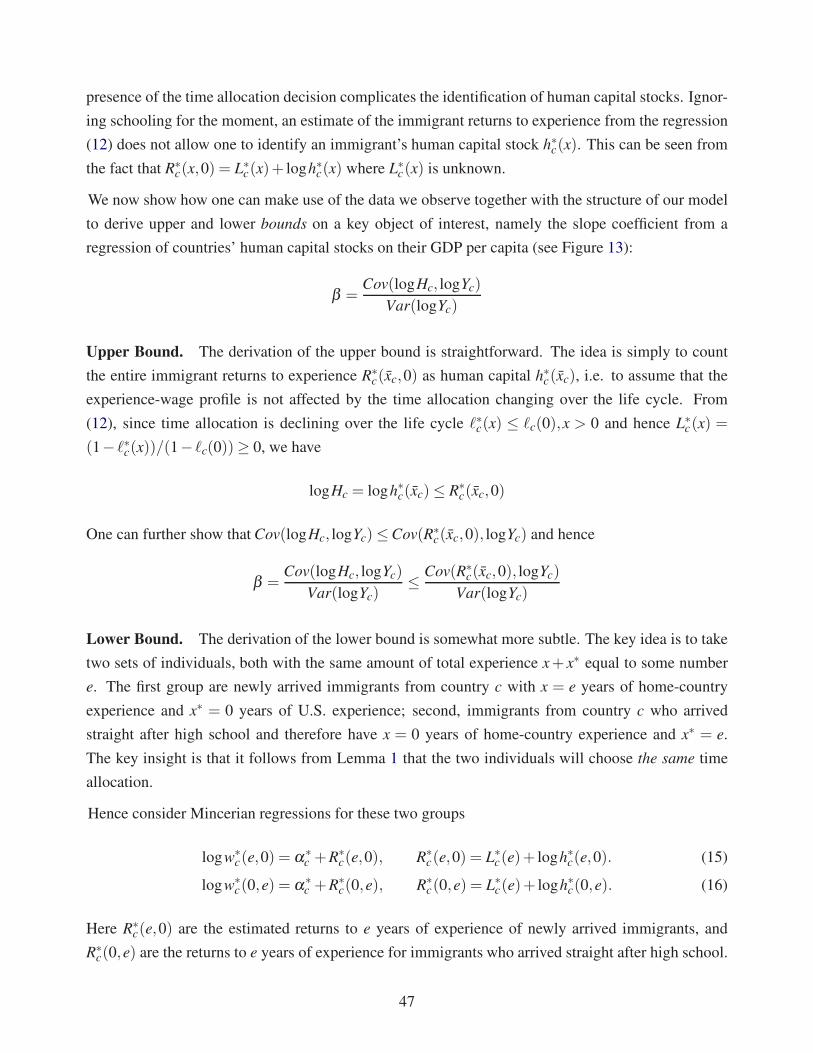
presence of the time allocation decision complicates the identification of human capital stocks. Ignor-

ing schooling for the moment, an estimate of the immigrant returns to experience from the regression

(12) does not allow one to identify an immigrant’s human capital stock h∗c(x). This can be seen from

the fact that R∗c(x,0) = L∗

c(x)+ logh∗c(x) where L∗c(x) is unknown.

We now show how one can make use of the data we observe together with the structure of our model

to derive upper and lower bounds on a key object of interest, namely the slope coefficient from a

regression of countries’ human capital stocks on their GDP per capita (see Figure 13):

β =Cov(logHc, logYc)

Var(logYc)

Upper Bound. The derivation of the upper bound is straightforward. The idea is simply to count

the entire immigrant returns to experience R∗c(xc,0) as human capital h∗c(xc), i.e. to assume that the

experience-wage profile is not affected by the time allocation changing over the life cycle. From

(12), since time allocation is declining over the life cycle ℓ∗c(x) ≤ ℓc(0),x > 0 and hence L∗c(x) =

(1− ℓ∗c(x))/(1− ℓc(0))≥ 0, we have

logHc = logh∗c(xc)≤ R∗c(xc,0)

One can further show that Cov(logHc, logYc)≤Cov(R∗c(xc,0), logYc) and hence

β =Cov(logHc, logYc)

Var(logYc)≤

Cov(R∗c(xc,0), logYc)

Var(logYc)

Lower Bound. The derivation of the lower bound is somewhat more subtle. The key idea is to take

two sets of individuals, both with the same amount of total experience x+ x∗ equal to some number

e. The first group are newly arrived immigrants from country c with x = e years of home-country

experience and x∗ = 0 years of U.S. experience; second, immigrants from country c who arrived

straight after high school and therefore have x = 0 years of home-country experience and x∗ = e.

The key insight is that it follows from Lemma 1 that the two individuals will choose the same time

allocation.

Hence consider Mincerian regressions for these two groups

logw∗c(e,0) = α∗

c +R∗c(e,0), R∗

c(e,0) = L∗c(e)+ logh∗c(e,0). (15)

logw∗c(0,e) = α∗

c +R∗c(0,e), R∗

c(0,e) = L∗c(e)+ logh∗c(0,e). (16)

Here R∗c(e,0) are the estimated returns to e years of experience of newly arrived immigrants, and

R∗c(0,e) are the returns to e years of experience for immigrants who arrived straight after high school.

47

Importantly note that, due to Lemma 1, the term reflecting the time allocation L∗c(e) is identical for

the two types of individuals.

Lemma 2 We have that

β =Cov(logHc, logYc)

Var(logYc)≥

Cov(R∗c(xc,0)−R∗

c(0, xc), logYc)

Var(logYc)(17)

where R∗c(xc,0) are the estimated returns to xc years of experience of newly arrived immigrants, and

R∗c(0, xc) are the returns to xc years of experience for immigrants who arrived straight after high

school.

Proof of Lemma 2 From the two regressions (15) and (16), we have R∗c(e,0)−R∗

c(0,e)= logh∗c(e,0)−

logh∗c(0,e). Further by the assumption that there is no skill loss when migrating h∗c(e,0) = hc(e) and

hence

R∗c(e,0)−R∗

c(0,e) = loghc(e)− logh∗c(0,e)≡ ∆ loghc(e)

That is, the difference between returns to experience of newly arrived immigrants, R∗c(e,0) and those

of immigrants who arrived straight after high school, R∗c(0,e) identifies the difference between the

human capital stock of non-migrants and those that migrated straight after high school.

Next, we explain how this can be used to obtain the lower bound (17). To fix ideas, consider first

the case B∗c = B∗ for all c, i.e. immigrants from all country learn at the same pace once they arrive

in the U.S. In that case, the human capital stock of individuals who spent their entire working life in

the U.S. h∗c(0,e) does not depend on their country of origin c. Therefore Cov(logh∗c(0,e), logYc) = 0

for all e and hence Cov(R∗c(e,0)−R∗

c(0,e), logYc) =Cov(∆ loghc(e), logYc) =Cov(loghc(e), logYc).

Given that Caselli (2005) documents that xc is approximately the same for all countries, then if we

assume B∗c = B∗ for all c, (17) would not only be a lower bound on the regression coefficient but an

exact expression.

More generally, we allow for the case B∗c 6= B∗ and in particular that immigrants from richer countries

face a higher B∗c . In that case, Lemma 1 implies that immigrants from richer countries accumulate

more human capital and hence Cov(logh∗c(0,e), logYc)≥ 0. In that case, one can only obtain a lower

bound:

Cov(R∗c(e,0)−R∗

c(0,e), logYc) =Cov(loghc(e)− logh∗c(0,e), logYc)≤Cov(loghc(e), logYc)

Using that Hc = hc(xc), we obtain (17).�

48

B.3. Proof of Lemma 1

We drop subscripts to ease notation, since we want to establish results for arbitrary Bc and B∗c . Without

loss of generality, we normalize ω = ω∗ = 1.

The Hamiltonian of the model is given by

H = h(1− ℓ)+λ (Bℓσ −δ )h

and the condition for optimality are

Hℓ ≤ 0, Hℓ (ℓ−1) = 0

λ = rλ −Hh

plus the terminal condition that the marginal value of human capital in the last period is equal to zero,

λ (T ) = 0. The solution is thus given by

h ≤ λσBℓσ−1h,[

h−λBσℓσ−1h]

(1− ℓ)≤ 0

λ = (r+δ −Bℓσ )λ − (1− ℓ)

λ (T ) = 0

and we notice that15 h cancels out in the optimality equation and so the solution is fully characterized

by (13) and (14).

The optimal training time ℓ(t), as long as the time constraint ℓ(t)≤ 1 does not bind, is the solution of

the differential equation

ℓ=

(

1

1−σ

)

[

(r+δ )ℓ− ((1−σ)B)ℓσ+1 −σBℓσ]

(18)

together with the terminal condition ℓ(T ) = 0. From (18), we have ∂ ℓ(t)/∂B < 0 for all t. Given the

terminal condition ℓ(T ) = 0, therefore ∂ℓ(t)/∂B for all t. Intuitively, the larger is B the faster ℓ is

going to decreases over time, and since we know that at time T , individual do not devote any time to

training, then going backward it must be that the higher is B the larger is ℓ at any point in time. That

h(t) and w(t)/w(t) are increasing in B follows immediately from their definitions. Finally, the last

part of the Lemma follows from the fact that the differential equation 18 that defines the path for ℓ(t)

is independent of h(t).�

15This is due to the assumption of constant returns in the human capital accumulation technology.

49

AFG

ALB

ARG

ARM

ATG

AUS

AUT

AZE

BEL

BGD

BGR

BHS

BIHBLR

BLZ

BMU

BOL

BRA

BRB

CAN

CHECHL

CHNCMR

COL

CPVCRI

CUB CZE

DMA

DNKDOM

DZA

ECU

EGY

ERI

ESP

ETHFIN

FRA

GBRGER

GHA

GRC

GRD

GTM

GUY

HKG

HND

HRVHTI

HUNIDN

IND

IRL

IRN

IRQ

ISRITA

JAMJOR

JPN

KEN

KHM

KOR

KWT

LAO

LBN

LBR

LCALKA

LTU

LVAMAR

MDA

MEX

MKD

MYS

NGA

NIC NLD

NOR

NPL

NZL

PAK

PAN

PERPHL

POL

PRI

PRT

ROM

SAUSDN

SGP

SLE

SLV

SOM

SWESYR

THA

TON TTO

TUR

TWN

TZA

UGA

UKR

URY

UZB VCT

VENVNM

YEM

ZAFZWE

0

.2

.4

.6

.8

Pe

rce

nta

ge

of

Se

co

nd

ary

Mig

ran

ts

500 1000 2500 5000 10000 20000 40000

PPP GDP p.c.

Figure 14: Secondary Migration Rate by GDP per capita

50