Life-Cycle Fertility and Human Capital Accumulation �

George-Levi GayleTepper School of Business, Carnegie Mellon University

Robert A. MillerTepper School of Business, Carnegie Mellon University

July 2012

Abstract

This paper analyzes the impact of policies expenditures on o¤spring and child carecosts investigating on life cycle fertility and female labor supply. We investigate sub-sidizing time spent on subsidizing expenditure on o¤spring, child care, both througha wage and also by directly child care, paying women who bear children a wage, andretraining them when they reenter the labor force after time spent out to raise chil-dren. To analyze these policies we formulate and estimate a dynamic model of laborsupply and fertility. The model accounts for maternal time spent raising o¤spring, plusthe e¤ect of time spent on current and summed discounted expenditures on them, Weestimate the model with the PSID data, and solve for the policy functions with theestimated parameters perturbed by policy innovations. Generally speaking all thesepolicies have a positive impact on fertility on almost all socioeconomic groups butretraining has the most pronounced increases on the birth rate.

1. INTRODUCTION

Both female labor supply and fertility behavior are topical issues of public interest. Forexample, the worldwide declining rates of fertility, especially amongst educated women,has consequences for intergenerational wealth transfers, along with the demand for publicinfrastructure and privately produced goods. And the persistence of the gender gap in U.S.wages, after a long period of shrinking, may have implications for employment discriminationlaws, and is a topic of continuing research for labor economists. Sociologists, demographersand economists recognize that female labor supply and fertility behavior are intertwined.So in principle public policies a¤ecting fertility should also a¤ect female labor supply, and

�Gayle acknowledges support from the Andrew Mellon Research Fellowship, while Miller was supportedby National Science Foundation Award SES0721098. We thank Elizabeth Powers for her comments, andwe have bene�ted from presentations at the Universities of Essex, Illinois (Urbana-Champaign), Kansas,Pittsburgh Wisconsin and Cowles Foundation, Yale.

vice versa. But quantifying the e¤ects of such policies and their implementation is quitechallenging.Social scientists have drawn upon all the usual tools in their attempts to predict how

public policies a¤ect fertility and female labor supply.1 Public opinion data, such as surveyresponses to hypothetical counterfactuals and ideal family size provide a �rst pass at howpopulations might react to policy innovations (European Commission,1990; Goldstein, Lutzand Testa, 2003). Time series analysis, for example over the post war period, have been usedto estimate the role of substitution and wealth e¤ects of increasing female wages on laborsupply and fertility (Butz and Ward, 1979, 1980; Buttner and Lutz,1990). Cross sectionalstudies, such as between OECD countries compare the e¤ects of di¤erent policies acrosscountries to address these issues (Billari and Kohler, 2004; Kogel, 2004). Event studies, sayrelated to the adoption of new programs have also been analyzed. (Milligan, 2005; Laroqueand Salanie, 2008; Cohen, Dejejia and Romanov, 2010).Our work joins a handful of studies that recognize the dynamic interactions between

female labor supply and fertility by modeling and estimating the sequential determinationof these joint events with panel data (Hotz and Miller,1988; Francesconi, 2002; Keane andWolpin 2010; Adda, Dustman and Stevens, 2011). The latter two also conduct counterfactualpolicy simulations. Keane and Wolpin investigate changes to the welfare system, whileAdda et al. simulate the e¤ects of increasing child allowances. We conduct counterfactualsimulations on four policies: Paying for expenditure on o¤spring; providing child care; payingwomen a wage to bear children; retraining mothers who quit the labor force when they reenterit.To analyze these policies we formulate and estimate a dynamic model of labor supply

and fertility. The model accounts for maternal time spent raising o¤spring and the e¤ectof time spent on current and summed discounted expenditures on them. We estimate themodel with the PSID data, and solve for the policy functions with the estimated parametersperturbed by the counterfactual policy innovations.Summarizing our results, all the policies we investigate increase total fertility rates (TFR)

on almost all socioeconomic groups but do not a¤ect labor force participation much. Re-training has the most pronounced increases in the birth rate, particularly amongst highlyeducated women. To amplify most of our 18 strati�ed groups have estimated TFR belowreplacement rate (say 2.1) under the current regime but if human capital lost from tem-porarily withdrawing from the labor force could be restored, than the TFR of all but onegroup (least educated unmarried white women) would rise to replacement rate.As a practical matter, our model predicts that a large proportion of human capital from

working experience is acquired within one working year. Therefore our model predicts thatretrospectively paying women the di¤erence between their wages in their �rst two years atwork after returning to work following an absence from work to give birth, would go a longway to raising the fertility rate of the most educated workers. More generally, subsidizingthis labor market outcome raises substantially fertility rates without a¤ecting participationrates very much. This serves to emphasize a point on the �rst slide: that public policy onthese issues must account for both the fertility and female labor market responses.The next section provides the theoretical underpinnings to our empirical investigations,

1For example see the recent survey by Gauthier (2007).

2

by laying out a life cycle model of labor supply and fertility. Then in Section 3 we brie�ysummarize the sample of households used in our empirical work, which is drawn from thePanel Study of Income Dynamics (PSID). Section 4 explains our estimation strategy, whileSection 5 reports our structural estimates. Then in Section 6 we conduct several policysimulations and summarize our �ndings. In Section 7 we conclude; all proofs and estimationdetails are contained in an Appendix.

2. A FRAMEWORK

In this model two kinds of human capital are accumulated, o¤spring and labor marketexperience. The bene�ts from bearing an additional child depend on the number and agesof its older siblings, while the time costs of raising the child are spread over several years.The value of past working experience is impounded in the current wage rate, and in additionleisure is not additively separable over time. Our model factors these considerations into adynamic optimization problem of female labor supply and fertility behavior.The model is set in discrete time, and measures the woman�s age beyond adolescence

with periods denoted by t 2 f0; 1; : : : ; Tg : The birth of a child at period t; a choice variable,is denoted by the indicator variable bnt 2 f0; 1g : There are two continuous choice variables,consumption xnt; and hours worked in the labor force, denoted by hnt 2 [0; 1]. To capturenonlinearities in leisure and returns to labor market experience, we de�ne the four discretechoice indicator variables that capture joint labor force participation and fertility choices as:

d1nt � I fhnt = 0g I fbnt = 0g ; d2nt � I fhnt > 0g I fbnt = 0gd3nt � I fhnt = 0g I fbnt = 1g ; d4nt � I fhnt > 0g I fbnt = 1g

where, for example, I fhnt = 0g is the indicator function for n staying out of the workforce inperiod t. Note that the choices are mutually exclusive and exhaustive, implying djnt 2 f0; 1gfor j 2 f1; : : : ; 4g with

P4j=1 djnt = 1:

2.1. Preferences

Births contribute directly to household utility. We assume that the spacing of births isrelated to preferences by the household over the age distribution of its children, as capturedby interactions in the birth dates of successive children. More speci�cally, let 0 denote theadditional lifetime expected utility a household receives for its �rst child, let 0 + k denotethe utility from having a second child when the �rst born is k years old, let 0 + k + jdenote the utility from having a third child when the �rst two are aged k and j years old,and so on. Thus the deterministic bene�ts from o¤spring to the nth household in period tare:

u(b)nt � bnt( 0 +

�bXk=1

kbn;t�k + b

TXk=�b+1

bn;t�k) (2.1)

Thus siblings k years apart are complementary in lifetime utility if k > 0:Apart from having utility for children, household utility also comes from its consumption

of market goods, denoted xnt; leisure, denoted lnt, and some random disturbances. Our

3

formulation incorporates both �xed and variable utility costs associated with working. Weassume the utility loss the nth female from working in period t are:

u(l)nt � (d2nt + d4nt) z0ntB0 + z0ntB1lnt +

�lXs=0

�slntln;t�s (2.2)

where znt is a vector that includes such variables as age, formal education, regional location,ethnicity and race. Thus B0 is a parameter vector characterizing the �xed-costs of partici-pating in the work force, and B1 shows the e¤ect of exogenous time-varying characteristicson the marginal utility of leisure. Preferences are increasing in leisure if:

z0ntB11lnt + 2�0lnt +

�lXs=1

�sln;t�s > 0

and concave if �0 < 0: The parameters �s for s = 1; :::; � capture intertemporal non-separabilities in preferences with respect to leisure choices. A value of �s < 0 for s = 1; :::; �means that leisure s periods ago increases the marginal utility of leisure, and results in lesswork and child care time today. Equivalently, a �nding of �s < 0 implies that current andpast leisure time are substitutes where as �s > 0 implies that current and past leisure timeare complements.The third component in utility is derived from current consumption. We denote by:

u(x)nt � ��1x�nt exp(z0ntB2 + �0nt) (2.3)

the current utility from consumption of xnt by household n in period t, and we assume"0nt is identically and independently distributed across (n; t) :We also allow for idiosyncraticfactors to a¤ect the utility from making the four distinct economic choices by assuming thereis a choice speci�c distrubance �knt that is identically and independently distributed across(k; n; t) as a Type 1 Extreme Value random variable.Letting � 2 (0; 1) denote the subjective discount factor over time, we de�ne realized

lifetime utility as:TXt=0

�t

(u(b)nt + u

(l)nt + u

(x)nt +

4Xk=1

dknt�knt

)(2.4)

2.2. Costs and Constraints

Raising children requires market expenditure and parental time. We assume that the dis-counted cost of expenditures from raising a child is �; a parameter that varies with householddemographics, and that a k year old requires nurturing time of �k up until age �c; and aconstant input per period denoted by � from then on.2 Letting cnt denote the amount oftime the nth household spends nurturing children in the household, our assumption aboutnurturing implies:

cnt =

tXs=0

�sbn;t�s (2.5)

2Thus o¤spring are di¤erentiated by market inputs but not by the input of their mother�s time.

4

where �s = � for all s > �c.3

Leisure in period t, denoted lnt; is de�ned as the balance of time not spent at work ornurturing children. It follows that the time allocated between nurturing children, marketwork and leisure must obey the constraint:

1 = hnt + lnt + cnt (2.6)

where hnt denotes the proportion of time worked in period t as a fraction of the total timeavailable in the period.Female labor market experience for the nth household in our sample is embodied in

the wage rate, denoted wnt; and depends on labor market experience and the demographicvariables znt. Let �nt denote the calendar year when the nth female is t years old, and let! (�) denote the wage of one e¢ ciency unit of labor. Following the literature real wages arethe product of ! (�) and an index capturing the number of e¢ ciency units embodied in aworker; we assume the mapping from experience to the current wage rate in year �nt is givenby:

wnt = ! (�nt)�n exp

"z0ntB3 +

�wXs=1

(�1shn;t�s + �2sd2nt + �2sd4nt)

#(2.7)

for some positive integer �: Thus Equation (2:7) shows that, in addition to the demographicvariables, the current wage depends on past participation and past hours up to � periodsago.Aside from the real wage wage ! (�), aggregate e¤ects are transmitted through interest

rates. We denote by � (�nt) the value of a consumption unit discounted back t periods, inother words the price of consuming in period �nt denominated in (�nt � �n0) consumptionunits, a notational convention we adopt so that the model can re�ect our emphasis on thelifecycle rather than on aggregate factors. Valued at calendar date �n0; net transfers tohousehold n at age t are then:

� (�nt) (xnt + z0nt�bnt � wnthnt) (2.8)

2.3. Optimization

We �nesse questions about how e¢ ciently markets and government interventions togetherallocate resources in this economy by modeling behavior as the solution to a social planner�sproblem. For appropriately de�ned interest rates � (�) and real wage rates ! (�), shadowprices that re�ect aggregate conditions and market clearance in general equilibrium, theplanner�s objective function is formed by summing the weighted expected value of utilityde�ned by Equation (2:4) over the lifetime of the woman and subtracting the discounted

3This speci�cation of maternal time inputs is broadly consistent with those considered in the literature.For example using data from time diaries, Hill and Sta¤ord (1980) found that maternal time devoted to childcare declines as the children age. Equation (2:5) implies that the child care process exhibits constant returnsto scale in the number of existing children. The evidence on the importance of such scale economies is mixed;Lazear and Michael(1980) �nd evidence of large scale economies while Espenshade(1984) �nds them to besmall.

5

sum of expected net transfers each period de�ned by (2:8). Denoting by ��1n the socialweight attached to individual n; Pareto optimal allocations are found by maximizing:

E0

"TXt=0

�t

u(b)nt + u

(l)nt + u

(x)nt +

4Xk=1

dknt�knt

!� �n� (�nt) (xnt + �bnt � wnthnt)

#(2.9)

with respect to fxnt; hnt; bntgTt=0; sequences of random variables that are successively mea-surable with respect to the information available at periods t 2 f0; 1; 2; : : : ; Tg, subject tothe individual household time constraints (2:6) and childcare demands (2:5).4

Setting � � max f�b; �l +M;�wg, the vector of state variables for the optimization prob-lem are:

Hnt � (t; z0nt;Mnt; bn;t��; :::; bn;t�1; hn;t��; :::; hn;t�1; �0nt; : : : ; �4nt)

Aside from demographics, Hnt captures the dependence of the current household state onlagged labor supply and birth choices. We denote the optimal choices solving (2:9) byfxont;hont; bontgTt=0, write dontk for the value of dknt implied by (hont; bont) ; and also set hknt �hk (Hnt) � hont for each k where h1nt = h3nt = 0.As shown in Sections 4 and 6 our estimators and policy functions are based on the

four discrete choices de�ned by birth and participation combinations, along with the �rstorder conditions for the continuous choices for consumption and hours worked conditionalon participation. Substituting (2:3) into (2:9) and di¤erentiating with respect to xnt yieldsthe (logarithm of the) Frisch consumption demand functions:

log xont = (�� 1)�1 (log �n + log � (�nt)� z0ntB2 � �0nt) (2.10)

Since the utility for xont is additively separable, its choice does not depend on the discretechoices dnt or the disturbance vector (�1nt; : : : ; �4nt) ; so the remaining parts of the solutionto the planning problem are determined separately.We now de�ne the deterministic components of current utility from leisure and births

when any discrete choice j 2 f1; : : : ; 4g is paired with hk (Hnt) : Substituting the optimal4There is a growing empirical literature that tests for deviations from Pareto optimal allocations, also

described as e¢ cient risk sharing, using panel data on individuals and households. See, for example, Altugand Miller (1990), Cochrane (1991), Mace (1991), Altonji, Hayashi and Kotiliko¤ (1995), Townsend (1994),Miller and Sieg (1997), and Mazzocco and Saini (forthcoming) Taken together, this body of work showsthat, depending on how the population for an agent is de�ned (such as village or caste, family or dynasty),the restrictions imposed by Pareto optimal allocations are quite hard to reject with panel data, unless oneassumes very limited forms of population heterogeneity, and also that preferences are strongly additive, twoassumptions that are widely regarded by microeconomists as being implausible. As a practical matter thereis little agreement amongst economists as precisely what departure from Pareto optimality should be adoptedwhen estimating models of individual and household behavior o¤ panels.

6

choice of hours worked into the implied utility from leisure:

u1 (Hnt) � 1�

tXr=1

�rbn;t�r

!"z0ntB1 + �0

1�

tXr=1

�rbn;t�r

!#

+

�lXs=1

�s

1�

tXr=1

�rbn;t�r

! 1� hn;t�s �

tXr=s+1

�rbn;t�r

!

u2 (Hnt) � u1 (Hnt)� h2 (Hnt)"z0ntB1 + 2�0

1�

tXr=1

�rbn;t�r

!� �0h2 (Hnt)

#

�h2 (Hnt)�lXs=1

�s

1� hn;t�s �

tXr=s+1

�rbn;t�r

!+ �n� (�nt)wnth2 (Hnt)

u3 (Hnt) � u1 (Hnt)� �0

"z0ntB1 + 2�0

1�

tXr=1

�rbn;t�r

!� �0�0

#

��0

"�lXs=1

�s

1� hn;t�s �

tXr=s+1

�rbn;t�r

!#� �n� (�nt) z0nt�

u4 (Hnt) � u3 (Hnt)� h4 (Hnt)"z0ntB1 + 2�0

1� �0 �

tXr=1

�rbn;t�r

!� �0h4 (Hnt)

#

�h4 (Hnt)�lXs=1

�s

1� hn;t�s �

tXr=s+1

�rbn;t�r

!+ �n� (�nt)wnth4 (Hnt)

Substituting in the optimal hours choices when the woman participates, we de�ne the currentt period expected value function for the leisure and birth choices as:

V (Hnt) � maxfdnsgTs=t

E

(TXs=t

4Xk=1

dkns�s�t [uk (Hns) + �kns] jHntj

)De�ning the conditional value function for each discrete choice as:

Vk (Hnt) � uk (Hnt) + E [�V (Hn;t+1) jdntk = 1; Hnt ]Bellman�s principle implies that for all j 2 f1; : : : ; 4g if doknt = 1 then:

Vk (Hnt) + �knt � Vj (Hnt) + �jnt (2.11)

Finally, when the woman participates in the workforce, meaning d2ns + d4ns = 1; then hoursof work (which depend on whether there is a birth or not), h2nt or h4nt;satisfy the �rst ordercondition:

z0ntB1 + � (�nt)wnt +@

@h2ntE [�V (Hn;t+1) jdknt = 1; Hnt ] =

�Xs=1

�s

1�

t�rXr=1

�kbn;t�r�s

!(2.12)

The estimation framework is directly based on our speci�cation of wages (2:7) ; the Frischdemands for consumption (2:10) ; di¤erences in the conditional valutaion functions (2:11)and the Euler equation that determines the number of hours work by women participatingin the workforce (2:12) :

7

3. Data

The data for this study are taken from the Family-Individual File, Childbirth and AdoptionHistory File and the Marriage History File of the Michigan Panel Study of Income Dynamics(PSID). The variables used in the empirical study are hnt; the annual fraction of hours workby individual n at date t; ewnt, her reported real average hourly earnings at t; xnt, real house-hold food consumption expenditures; FAMnt, the number of household members; Y KIDnt,the number of children less than six years of age; OKIDnt, the number of children of agesbetween six and fourteen; AGEnt, the age of the individual at date t; EDUnt, the years ofcompleted education of the individual at time t; HIGH:SCHnt; completion of high schooldummy; BLACK and HISPANIC race dummies for blacks and Hispanics, respectively;NEnt; NCnt,SOnt, which are region dummies for northeast, northcentral, and south, respec-tively, and MARnt; denoting whether a woman is married or not. The construction of oursample and the de�nition of the variables is described in greater detail in Appendix 3.Table 1 contains summary statistics of our main variables. The sample has aged, house-

hold size has declined, and the decline is most pronounced amongst young children. Thesteep decline in household size over the two decades, and the aging evident in the sample,relative to aggregate trends in the US, largely re�ects the sampling mechanism of the PSID.Thus we cannot infer any aggregate trend in fertility from this table. Household income hasincreased somewhat, but household consumption of food has declined. However, both foodconsumption and income per capita has increased over the sample period. More striking isthe rise in female income, which greatly outstrips increases in household income. This is dueto both higher wages and greater hours. Because schooling has not increased over the sampleperiod, the number of years of formal education is not a factor in explaining aggregate trendsin female wages and labor supply, or any changes that might have occurred in fertility.

4. Estimation

Our estimation strategy essentially follows Altug and Miller (1998) by extending their frame-work of female labor supply and human capital accumulation to incorporate choices aboutfertility. First we estimate the wage equation, and in the process recover the individual �xede¤ects from the wage equation. Then we estimate the social weights of the social planner�sproblem from the Frisch demand for consumption. Both that determine the conditionalchoice probability (CCP) mappings, which are estimated nonparameterically as a mappingof the �xed e¤ects are arguments that along with the state variables and demographic char-acteristics that determine them. The structural parameters are estimated from equationsthat exploit the �nite dependence properties of this model, and our standard errors accountfor the sequential estimation method.

4.1. Wages

We assume that the reported wage rate, denoted ewnt (for the nth household in period t)measures the woman�s marginal product in the market sector with error, so that:

ewnt = g( eAnt) exp(e�nt) (4.1)

8

where the multiplicative error term in equation (4.1) is conditionally independent over people,the covariates in the wage equation and the labor supply decision. Taking logarithms onboth sides of Equation (4.1), and then di¤erencing, yields:

4e�nt = 4 ln( ewnt)� �Xs=1

(�1s4hn;t�s + �2s4dn;t�s)�4z0ntB3 �4!t (4.2)

which we estimated with a linear instrumental variables estimator.

4.2. Consumption preferences

In our model, the e¤ects of di¤erences in wealth across households on their fertility andlabor supply decisions is determined a single parameter, their weight in the social planner�sproblem. The inverse of their social weight is their marginal utility of wealth, and it can beestimated with household data on consumption. Taking logarithms of (2.10) and then �rstdi¤erencing yields:

(1� �)�14 �0nt = 4 ln(xnt)� (1� �)�14 z0ntB2 + (1� �)�1 ln(�t) (4.3)

The assumptions in Section 2 imply that the unobserved variable "5nt is independent ofindividual speci�c characteristics, implying:

E(�4 ln(xnt)� (1� �)�14 z0ntB2 + (1� �)�1 ln(�t) jznt

�= 0

which can be exploited using a linear instrumental variable procedures similar to the esti-mated wage function.

4.3. Individual-speci�c e¤ects

We assume the �xed e¤ects �n and �n are mappings of the household�s permanent character-istics zn, denoted by � (zn) and � (zn) respectively. They can be estimated nonparamatricallyas level e¤ects o¤ the wage equation and the �rst order condition for consumption. Let:

�1nt � ln (ewnt)�X�

s=1(�1shn;t�s + �2sdn;t�s)� z0ntB3 � !t = � (zn) +e�nt

�2nt � ��ln(xnt)� (1� �)�1z0ntB2 + (1� �)�1 ln(�t)

�= � (zn) + �0nt (4.4)

By assumption both e�nt and �0nt are orthogonal to zn; from which it follows that � (zn) =E [�1nt jzn ] and � (zn) = E [�2nt jzn ]. We estimate � (zn) and � (zn) with Kernel regressions o¤the cross section, using consistent estimates of the wage and consumer preference parametersobtained in the previous stages of the estimation.

4.4. Labor force participation and fertility

Our estimation equations for labor force participation, hours worked and fertility behaviorare based on the �nite dependence property of the model, which provides a computationallyconvenient expression for the conditional valuation functions described in the next section,

9

and the logit form of the conditional choice probabilities in the valuation functions. Finitedependence arises in this model because it is feasible for women to avoid pregnancy and notwork each period, and from her perspective in the model, she would no longer care abouther work or birth history if she has not worked for at least the previous � periods and allher children were at least � years old.To demonstrate the �nite dependence property, we now de�ne four choice paths � + 2

periods into the future that a woman might take starting at period t, and the history ofstate variables they generate, denoted by H(s)

knt for k 2 f1; : : : ; 4g and s 2 f1; : : : ; �+ 2g, andde�ned as:

H(s)1nt �

�z0nt+s;hn;t��+s; :::; hn;t�1; 0; :::; 0; bn;t��+s; :::; bn;t�1; 0; 1; 0; :::; 0

�0H(s)2nt � (z0nt+s;hn;t��+s; :::; hn;t�1; h2nt; 0; :::; 0; bn;t��+s; :::; bn;t�1; 0; 1; 0; :::; 0)

0

H(s)3nt � (z0nt+s;hn;t��+s; :::; hn;t�1; 0; :::; 0; bn;t��+s; :::; bn;t�1; 1; 0; :::; 0)

0

H(s)4nt � (z0nt+s;hn;t��+s; :::; hn;t�1; h4nt; 0; :::; 0; bn;t��+s; :::; bn;t�1; 1; 0; :::; 0)

0

Note that all four histories evolve by choosing d1n;t+s = 1 for s > 1, namely not participatingin the labor force and not giving birth. H(s)

1nt denotes the state variables for the problem atperiod t+ s when a woman makes choices d1n;t+1 = 1 and d3n;t+1 = 1 in periods t and t+ 1.H(s)2nt only di¤ers from H

(s)1nt by setting d2nt = 1 (and hnt = h2nt). Both H

(s)3nt and H

(s)4nt set

d1n;t+s = 1 for all s > t; H(s)3nt sets d3nt = 1 while H

(s)4nt sets d4n;t+1 = 1. By construction it

follws that for all k 2 f1; 2; 3; 4g:

H(�+2)knt = (z0n;t+�+2; 0; :::; 0; 0; :::; 0)

0 � Hn

showing that it is feasible to reach a point � + 2 periods hence, where di¤erences in twochoices in periods t and t + 1 (equalizing family size) followed by a sequence of the samechoice (not to work) obliterate any future consequences of choices prior to period t.To show how �nite dependence is exploited in the representation of the conditional value

function and hence in estimation, de�ne l(s)knt � ln;t�s for all s 2 f�1; : : : ;��g ; and fors 2 f0; 1; : : : ; �+ 1g let l(s)knt as the amount of leisure consumed in period t + s when thischoice path indicated by the state variables H(s)

knt is followed. For example:

l(s)ntk =

1�

tXk=1

�kbn;t�k � �k

!

The leisure component of utility acruing over the periods t+1 though S from setting dn;t+j;1 =1 each period t+ s is thus:

�n

��1Xs=1

�s

"z0n;t+jB1l

(s)ntj +

�Xr=1

�sl(s)ntjl

(s�r)ntj

#

The following Lemma now provides a characterization of the conditional valuation functions.

10

Lemma 4.1. De�ne for k 2 f1; : : : ; 4g:

Wk (Hnt) =

T�tXs=1

�s�t

(z0n;t+sB1l

(s)ntk +

�Xr=1

�sl(s)ntjl

(s�r)ntj

)��

�Xs=1

�s�t ln p1

�H(s)knt

�+��+2�tV (Hn)

Then:

Vk (Hnt) =

�uk (Hnt) +Wk (Hnt) for k 2 f3; 4guk (Hnt)� z0n;t+1B0� +Wk (Hnt) for k 2 f1; 2g

and for j 2 f1; : : : ; 4g:

Vj (Hnt)� Vk (Hnt) = � ln pj (Hnt)� � ln pk (Hnt) (4.5)

The log odds ratio scales the di¤erence in conditional value functions by a varianceparameter because of wages. Similarly the correction factor on the the choice probabilitiesthat o¤set the di¤erence between the conditional valuation functions and the (unconditional)value function. Equating the right side of both. Di¤erentiating

5. Results

This section reports on the results of the structural estimation. Tables II through VII containestimates of estimates of the parameters determining wages, consumption preferences, theparticipation cost, the child nurturing time, plus the utility from leisure and o¤spring.

5.1. Wages

Our estimates of the wage equation, displayed in Table III, are comparable to those reportedin Miller and Sanders (1997) for the National Longitudinal Survey for Youth (NLSY), Altugand Miller (1998) also using the PSID, and others. All the coe¢ cients are signi�cant. Work-ing an extra hour increases the wage rate up to four years hence, although in diminishingamounts. The e¤ect is nonlinear, and this is captured by the participation variables. Agehas a quadratic e¤ect, eventually leading to declining productivity, and additional educationmitigates the onset of the decline. We note that the linear terms on age are not identi�ed.The estimate quantitative magnitudes of past experience are also plausible. Recent work-

ing experience is more valuable than more distant experience: at 2000 hours per year, thewage elasticity of hours lagged once is about 0.18, but the wage elasticity of hours laggedtwice is only 0.03. Also the further back the work experience is, the less the timing matters;an extra hour worked one year in the past has about twice the e¤ect on current wages as anextra hour worked two years in the past, but the di¤erence between the wage e¤ects of anextra hour worked three and four years in the past, respectively, is less than 40%.Another measure of the e¤ect of past labor supply on wages: consider the total change

in wages for a woman who has not worked up to date t � � and then works the sampleaverage of hours for those women who work, denoted ht: Then this measure is given byP4

s=1[�1sht�s + �2s] = 0:12: Much of this long-term e¤ect is due to hours worked in thepast year. Speci�cally, the growth in wages between t� 1 and t for a woman who does notparticipate from t� � to t� 2; but works the sample average at t� 1 is �11h;t�s+ �21 = 0:08.

11

On the other hand, women who worked less than 1000 hours the previous year do not receivethis increase in wages, this may be capturing the e¤ect of discouragement normally found inthe standard job search model. It should be noted that we do not explicitly model this typeof search cost in our model, however, we can pick up the lower bound of this e¤ect. Thismeans that not everybody gets the bene�t from past job experience, there is a thresholdnumber of hours of about 1500 for this positive e¤ect to kick in. This will impact fertilitybehavior even more than if there were positive bene�t from all levels of past hours, since amother could reduce her hours and still continue to enjoy the bene�t of higher future wages.We will come back to this point in the empirical �ndings section when we will have estimatesof the fraction of time a mother spends nurturing her new born.The estimated change in aggregate wages over our sample period is displayed in Figure I,

along with its 99% con�dence interval. The most striking feature of that plot is that althoughthe magnitude of the changes �uctuate over the sample period, the signs are always positive.This shows that over time the aggregate females wage has been increasing. This is not asurprising �nding, given the fact the wage gap between males and females having been closingover time. However it does raise an interesting issue as to whether the attachment of femalesto the labor force, in term of their persistence in labor participation, is having an aggregatee¤ect. For example, suppose by more females working more hours and participating on amore consistent level equivalent to men, then the employers in the aggregate are willing topay females higher wages closer to males. This higher wages, some would argue, would thencause females to work more and have less children. Our approach can also disentangled sucha result by controlling for aggregate shock, and then seeing the relative importance of thewage e¤ect.

5.2. Preferences over Consumption and Wealth E¤ects

The estimates of the consumption equation are based on the main sample of females forthe years 1968 to 1992. Consumption for a given year in our study is measured by taking0.25 of the value of the di¤erent components for year t � 1 and 0.75 of it for year t. Thisis explained in more detail in the data appendix. The elements of znt used in this stageof the estimation are de�ned as FAMnt; Y KIDnt; OKIDnt; AGE

2nt; NCnt and SOnt: The

estimates in Table 4 show that consumption increases with family size and children consumeless than adults, since the coe¢ cients on children between the ages of zero and fourteenare negative and smaller in absolute magnitude than the coe¢ cient on total household size.Furthermore, the behavior of consumption over the life-cycle is concave since the coe¢ cienton age squared is negative. All the other coe¢ cients are signi�cant. The agregate shockscomponents are estimated very precisely. In fact, there is also signi�cant variation over timeas the test statistic for the null hypothesis that (1� �)�1� ln (�t) = (1� �)�1� ln (�t�1)for t = 1969; :::; 1992 is 395. Under the null hypothesis, it would be distributed as a �2 with23 degrees of freedom, implying rejection of the null at 99% signi�cance levels.

5.3. Fixed Cost of Participation

Table VI contains estimates of the �xed cost of participation. First the constant term isnegative, which means that participation in the labor force has a �xed utility cost instead

12

of a bene�t, which is what standard economic theory would predict. Age reduces this costof participation in the labor, but this reduction is at a decreasing rate as the parameterestimate on the AGE2 is negative. Education decreases the cost associated with age. Thereis a positive sign on the estimates of AGE�EDUC which implies that a more educated femalehas a lower cost of participation for a given age than a less educated female. To understandthe overall e¤ect of age and education on the �xed cost of participation, we investigate whatis the shape of this function conditional on education. Married women have a lower cost ofparticipation while blacks have a higher cost of participation for a given age and educationlevel. Again these results are not surprising since the standard literature has documentedsimilar results( see for example Altug and Miller (1998))..

5.4. Nurturing Cost

Table VII contains the results from the estimation of the fraction of time spent nurturing achild. These estimates seems quite small and the only signi�cant cost is that of older children.These are similar results to those found by Hotz and Miller (1984) which found that theseparameters follow o¤ a geometric rate. This is very important in our model, since with thenonlinearity observed in the estimates of the wage equation, this implies that if a femalereduces her time in the labor force to have a child, then they would not bene�t from theincreases in wages as a result of human capital accumulation in terms of their previous laborsupply. So holding all other things constant, this would make having children less desirablefor a female who is on a high wage trajectory. This combined with the estimates of the riskaversion parameter means that females would like to smooth more there consumption, henceworking more in earlier years and delaying child-bearing to later years. This would meanthat working females would have less children than nonworking female.

5.5. Utility Cost of Leisure

Table VIII contains the estimates for the utility cost of leisure. Leisure have the expectedsign, the direct e¤ect of age and age square are both insigni�cant. However, for a givenage education increases the value of leisure, this e¤ect is working in the opposite directionfrom these for participation. This mean that for given age a female with higher educationparticipate more but conditional on participation the would take more leisure. Our estimatessuggest that leisure is intertemporally nonseparable. Past leisure are substitute with forcurrent leisure These is opposite to what is found in Altug and Miller (1998), among other,about the separability of leisure when one does not control for children. Another, surprisingresults we found is that the sign on marriage in our results is negative. At �rst glance, thiswould imply that married females love leisure less. One explanation for this e¤ect could besimple the fact that married females are working more than before and is still having children.Since we do not allow at the moment for the utility of birth or the time cost of raring a childto depend on such demographics, as marital status, then the only way they found then behaving children and still working is if they as a group love leisure less. Another explanationmay be due to the welfare system. In the era of our sample, a subsistence income (AFDC)is available to unmarried mothers, but (basically) only conditional on them not working.Married females do not face a similar trade-o¤. Since welfare participation among female

13

heads is quite common in this era (roughly around one-third), this is de�nitely an importantenough phenomenon to account for this results. In short, the �leisure�time of female headsis highly subsidized, and they may well have similar preferences as wives.5 This is something that we will explore further.

5.6. Birth E¤ects

We concurred with the classical literature that children are good and not bad, since we �nda positive net utility all birth except for the child. It should be noted that this is the nextbene�t all this suggest is that women prefer two children to one. The parameter on thetiming of births for example, would imply that the optimal space of a two-child family wouldbe 3 to 4 years apart. So, having children too close or too far apart is less desirable. Turningto the cost of a child, we �nd that both sets of estimates give similar results. We �nd thathaving at least a high school education signi�cantly increases that cost. After controllingfor education, we �nd that Blacks have a signi�cantly lower cost than White. The factthat education signi�cantly increases the cost of having a birth coincides with our earlierhypothesis, and can help explain the unanimous empirical �nding that number of childrenis negatively related to level of education.

6. Policy simulations

There are many ways in which public policy over the last century has a¤ected the costsand bene�ts of having children. From child labor laws to the public provision of schooling,from the subsidizing of health care to local taxes that support amenities such as swimmingpools, as well as sporting and other events for children, raising children depends on socialinfrastructure that is often taken for granted in modern developed societies. Over the lastseveral decades, greater attention has been paid to jointly determining fertility and femalelabor supply. Part of the concern about the falling rates of fertility are related to the long-term viability of the social security system in many developed countries, especially inWesternEurope.This section considers a variety of policies that subsidize fertility to investigate how re-

sponsive women are to changes in the incentives they factor in between market work andraising a family. Our study shows that di¤erent policies not only have di¤erent aggregateor average e¤ects on fertility and female labor supply, but also have very signi�cant compo-sitional e¤ects, or incidence across this heterogeneous population. We hasten to add thatour contribution is positive, not normative, seeking to provide quantitative analysis againstwhich di¤erent policy options can be evaluated.

6.1. Overview of the simulations

We substituted the parameters obtained from our estimation procedures into the utilityfunction, the equation characterizing the returns to experience, and the child care costequation and solved the decision-maker�s problem. We conducted simulations for a wide

5We would like to thank Elizabeth Powers for pointing out this very insightful possibility to us.

14

range of female types in the population, but they are not exhaustive. We strati�ed thepopulation, breaking down the groups according to a three-way classi�cation scheme, byrace, marriage and education, and considered an individual whose unobserved �xed e¤ectscorrespond to the estimated means of the distributions. Three racial types were considered,namely Black, White and Hispanic (respectively abbreviated B, H and M in Tables IX andX below). Marriage was a dichotomous variable partitioning women by marital status at age25, where M denotes she was married at age 25 or before, and U if not. We considered threeeducational groups, those who completed some years at college (denoted by the inequalitysign >), those who completed some years at high school but not college (denoted by HS), andthose with less education than that (denoted by a < sign). Thus our simulations apply towomen in the 18 categories whose marginal utilities�of wealth, and whose endowed marginalproduct of labor (controlling for schooling and experience), correspond to the estimatedsample means.The models we simulated are slightly less complex than the estimation framework itself

in three ways. The �rst simpli�cation was to limit the choice set. Rather than assuming thatworkers made a discrete choice about whether to participate in the labor force or not with acontinuous hours choice, we discretized the labor supply choice set facing workers, limitingthem to 10 equally spaced choices in the [0; 1] interval. Second, we linearized the value ofmarginal consumption around the marginal utility of consumption achieved in the currentregime. Thus in the objective function (2.9), U3ntk is replaced with eU3ntk � ��1n : Third, weinvestigated an economy where there are no aggregate shocks. As a practical matter, thequantitative signi�cance of aggregate demographic shocks (such as the baby boom in theU.S., the AIDS crisis in Botswana and other countries, the e¤ects on fertility of immigrationboth legal and illegal into U.S. and parts of Western Europe) is di¢ cult to overstate, and wethink that excluding them is the main reason why our results should be treated cautiously.The model was solved for each group under �ve policy regimes. The benchmark regime,

labelled Estimation, is the current one, which may be compared with the conditional samplemeans from the data set. In the �rst two alternative regimes we analyze the subsidy tohaving children does not vary with the recipient, although the value a mother places on thescheme depends on her wealth and wage rate. In the regime labelled Expenses, the statepays all the estimated monetary costs associated with raising children, removing the wedgein the marginal utility of wealth between households that have children and those that donot. Under the Day-care policy, maternal time is replaced with publicly funded child carecenters. In the other two regimes the payment mothers receive depends on her wages andhours she worked before taking time o¤ to have a child. The Wages policy would pay themother the wages she would have received if she had decided against having her child. Ifthe Retraining policy is adopted, mothers are given retraining upon reentering the workforcethat fully restore the human capital from lost workforce experience.In our model there are three costs associated with child-care: the lifetime discounted cost

of market inputs used up raising a child, the direct time cost in terms of the required fornurturing, and the human capital accumulation cost stemming from the experience acquiredfrom working that is not used when women quit the labor force to have children.

15

6.2. Solving the Model

The Type 1 extreme value also implies that for each j 2 f1; : : : ; 4g

Vj (z�nt) = u

(b)ntj + u

(l)ntj

�h(j)nt

�� � (�nt)

��bntj � wnth(j)nt

�+ � log

(4Xk=1

expVk

�z(j)n;t+1

�+

)Upon de�ning pknt as the conditional choice rate in period t, we obtain the probabilityof making choice k by the nth female in period t as:We also use the fact that an interiorsolution for those participating in the labor force requires @V1ntn@hnt = 0 or @V3ntn@hnt = 0:Di¤erentiating with respect to hours we have:Thus if Ioknt = 1 for k = f1; 3g , then hont solves:

� (�nt)wnt � z0ntB1�1� c(j)nt � h

(j)nt

��

�Xs=0

�slnt�s =

4Xk=3

pk (z�nt)@Vk

�z(j)n;t+1

�@h

(j)nt

(6.1)

The left side of Equation (6.1) gives the current bene�ts and costs of spending a marginalhour working, comprising a utility cost in terms of leisure foregone, and the value of the extragoods and services produced. The right side shows the expected future bene�ts. Marginallyadjusting current hours worked directly a¤ects future productivity as well as the bene�ts offuture leisure. Moreover, supposing the probability of working next period increases nextperiod from this adjustment, the net bene�ts of working next period should be applied tothe increase. This is captured in the second expression on the right side of Equation (6.1).We �rst simulated the prediction of the model for females in each of the categories

described above over the 25 years of a partial life cycle starting at age 20, for use as a benchmark case. This requires us to solve 18 valuation functions for the optimization problemeach type solved, obtain the optimal decision rules, and thus compute the probabilities ofobserving any given decision, as a mapping of the state variables, which in this case arethe vector of lagged labor supplies and a vector for the ages of the o¤spring. An appendixdescribes the algorithm in detail. Brie�y, we combined the use of both policy functioniteration (using Newton steps) with value function iteration (using the contraction operatoron the value function). Convergence to the solution of the in�nite horizon problem occurredrelatively quickly, typically within seven iterations.The labor force participation rate and expected fertility rate over this period (essentially

the TFR) for each type is reported in the second column of Tables IX and X under theheading of Estimation. A sense of how representative our groups are is found by comparingthe simulated results for our estimated model with their corresponding sample means in the�rst column, headed Actual. Note that the numbers are not very close, although many of theinequalities within each column are preserved. This is attributable to two factors. The �rstis estimation error. The second is that the sample means do not condition on the values ofthe unobservables, which enter in a highly nonlinear way into the participation and fertilitychoices. To separate out these separate in�uences, we will nonparametrically estimate thesame set of statistics for that person in the group with the estimated mean �xed e¤ects,which simply weights the data used to obtain the averages in the �rst column by how closeeach observation is to the mean estimated �xed e¤ect vector.Table IX shows most of the types have fertility rates below the replacement rate of 2.

For example, the TFR of all the college educated groups are all below the replacement rate.

16

College educated white females bear the least number of children (1.1 for the group as awhole and 1.2 at the mean �xed e¤ects), and black married females with less than highschool education the most (2.1 for the overall group and 2.4 at the mean �xed e¤ects).In most, but not all groups, those married by 25 bear more children than those who had

not married by then. Table X shows that, with the notable exception of college educatedwhites, unmarried women are more likely to participate in the labor force. At 0.93, the laborforce participation rate for a married college educated white female with the mean �xede¤ects exceeds all other groups, closely followed by unmarried college educated black women(at 0.91). Across education achievement and marital status but within race categories, blacksexhibit the biggest range in labor force participation rates. The exact derivation is presentedin more details in Appendix 1.

6.3. Child-care Support

There are many ways to subsidize fertility by having the state pay for the discounted lifetimecost of children. For example, it could be achieved though tax credits at upper income levelsand child support payments for those who do not receive enough taxable income. In thisframework this is equivalent to imposing the constraints �0 = 0 and �1 = 0 in the expressionfor child care costs:

� (znt) = �0 + z0nt�1

The total fertility and labor force participation rates that are induced by this subsidyare shown in the third columns of Tables IX and X. Paying the market goods inputs forraising children has a substitution and wealth e¤ects. In a static model, the substitutione¤ect induces women to have more children and reduce their own consumption of leisure andother goods, while the wealth e¤ect induces them to increase their consumption of leisureand children. The results of the dynamic simulations lend support to this intuition. In16 of the 18 groups labor force participation declines, and in all but one instance fertilityrises, 6 groups (compared to 4) now settling above the replacement rate. The 3 types whosefertility behavior is most sensitive to this policy shift are the married non-college educatedblack female and the unmarried lowest educated black female. By way of contrast the biggestreduction in labor force participation rate is amongst unmarried high school educated whites.

6.4. Day-care

Rather than pay for market inputs directly, another public policy for subsidizing fertility isto expand the availability of child care services for the mothers of infants and preschool agechildren, by �nancially supporting centers, or reimbursing mothers who place their childrenin them. In our framework a policy that eliminates the maternal time inputs altogether wouldset �i = 0 for i 2 f1; : : : ; 5g : This increases the amount of time mothers of young childrenhave for leisure and work. In a static model of fertility and labor supply, fertility increasein response to a reduction in one of its factor inputs, maternal time. Furthermore, the timefreed up from looking after children is distributed between extra leisure, and working for moregoods and services over and above those used up by the additional children. Consequently,one predicts that both fertility and labor supply would increase, the latter less than theamount of time released from child care.

17

The fourth column shows the labor force participation and fertility outcomes from solvingthe optimization problem under the Day-care policy. As expected all the group exhibithigher fertility rates, 12 now at or above the replacement rate of 2.0, with married highschool educated white females registering the biggest increase (from a TFR of 1.52 to 2.30).Comparing the e¤ects on TFR across di¤erent groups, we see that switching from subsidizingmarket inputs to replacing maternal time inputs has a far greater impact on females withsome college education than those who did not complete high school. Indeed in just onegroup, married blacks who did not complete high school, TFR would actually fall from 2.63to 2.41 if subsidizing market inputs were replaced with subsidizing maternal inputs. This�nding demonstrates that the type of subsidy to child care helps determine not just theaggregate level of births, but also their composition within di¤erent types of households.The change in labor force participation rates are more ambiguous, in fact puzzling. Since

returns from experience on the job is likely to strengthen attachment to the labor forcebeyond that predicted by the static model, we are further investigating this counter-intuitiveresult.

6.5. Paid Maternity Leave

Paying females wages when they take maternity leave is a third way of promoting higherfertility. A distinguishing feature of this policy is that women with high wages receive greaterpayment than those receiving lower wages. (Note that if the payment is a �xed allowance,then the analysis of Expenses policy applies.) In contrast to the two previous schemes, (eachof which has only one degree of freedom, the proportion of costs or time covered), this schemehas two, what percentage of her market wage a mother is paid while on maternity leave, andthe maximum eligibility period per child. Under the Wages policy, mothers are paid thewage they would have received if they had not given birth, and the maximum eligibilityperiod is the amount of time they would have withdrawn from the workforce in the absenceof the subsidy. These variables are for the most part negatively correlated, and thereforea¤ect the total payment in o¤setting directions.In particular, suppose the woman gives birth at period t; let hon;t+s (bnt = 0) denote the

woman�s labor supply s periods after the birth had she not left the workforce to give birth,let won;t+s (bnt = 0) denote her wage rate had she not given birth, and let �

0n denote the

number of periods she would have taken o¤ if there were no provisions for paid maternityleave. Then in this policy regime the wage payment she receives upon having a child is:X�n

s=0�n;t+sw

on;t+s (bnt = 0)h

on;t+s (bnt = 0)

In a static framework, paid maternity leave induces women to reduce their labor supplyand have larger families. In our dynamic framework paying wages does not fully compensatea mother for taking maternity leave, because job market experience acquired before givingbirth depreciates over the time spent out of the labor force. Consequently, females whodecide to have a child because of the paid maternity leave may simply exit the labor forcepermanently if their market capital has depleted su¢ ciently quickly. This scenario certainlyarises when, in the absence of the paid leave policy, women essentially choose between havinga career and having a family.

18

Our preliminary simulation results are displayed in the �fth columns of Tables IX and X.They show that in 13 out of the 18 cases the labor supply participation falls, because of thesubstitution e¤ect into child rearing activities, and the compounding e¤ect of human capitaldepletion. Although total fertility rates increase in all categories, this policy is not as e¤ectiveas directly paying for the time inputs; in every category fertility rates under subsidized Day-care exceed those in attained when there is paid maternity leave as mandated in Wages.

6.6. Retraining

In our framework mothers lose human capital from temporarily withdrawing from the laborforce. The last counter factual regime we consider does not make any payments to mothers,but o¤ers partial compensation by putting women returning to work from maternity leaveon an equal footing with those who chose not to have children. The policy scheme simulatedin Retraining restores them to the wage trajectory they would have been on if they notwithdrawn from the workforce to have children. In our framework the labor force experienceover the previous � periods helps determine the current wage. Thus, if the female in Model4 reenters � 4n periods after she has her birth, the natural logarithm of her wages increasesby: Xminf�;�4ng

s=0

��1sh

on;t�s (bnt = 0) + �2sd

on;t�s (bnt = 0)

�The last columns of Tables IX and X display the results, which in some ways are the

most dramatic. The total fertility rate of every group except the unmarried white femaleswith less than high school education rises above the replacement rate, and for one group,married black females with high school education, reaches 3.

7. Conclusion

This paper develops a dynamic model of female labor supply and fertility behavior andestimates its structural parameters. Previous empirical research on female labor supply hadshown that current labor supply choices a¤ect future wages and utility through intertemporalnonseparabilites in the production function (such as through learning by doing or staying inpractice), and in utility (for example, through the household production function and alsopossibly due to the intertemporal nature of utility from leisure). In addition, there are asmall number of studies of fertility behavior that suggest the timing of later births is partlydetermined by economic factors. Our study nests both kinds of dynamic interactions withina uni�ed structural model.Our estimates rea¢ rm the importance of dynamic factors in labor supply and fertility

choices. Wages increase with experience up to four years in the past, recent experiencecounting the most. Leisure taken in di¤erent periods are substitutes. Estimated preferencespeg optimal birth gestation at about two years.From a policymaker�s perspective: Restoring human capital from work experience is the

biggest factor in raising TFR, even though this does not directly subsidize childbearing andfertility inputs. Paying for daycare, expenses incurred raising children, or women a workingwage while they have children, all increase fertility rates. None of the policies have muche¤ect on labor supply, which is largely determined by the human capital considerations.

19

References

[1] Ahn, Namkee(1995), Measuring the Value of Children by Sex and Age Using a DynamicProgramming Model, Review of Economic Studies 62, 361-79

[2] Altug, Sumru and Robert A. Miller (1998), The E¤ect of Work Experience on FemaleWages and Labour Supply, Review of Economic Studies, 45-85.

[3] Altug, Sumru and Robert Miller(1990), Household Choices in Equilibrium, Economet-rica, Vol. 58. no. 3., 543-570.

[4] Angrist, J. and W. N. Evans( 1998), Children and Their Parents� Labour Supply:Evidence from Exogenous Variation in Family Size, American Economic Review 88,450-77.

[5] Arroyo, Cristino R. and Junsen Zhang (1997), Dynamic Microeconomics Models of Fer-tility Choice: A Survey., Journal of Population Economics, Vol.10, 23-65.

[6] Becker, G. (1965), A Theory of Allocation of Time, Economic, Journal, 75, 496-517.

[7] Becker, Gary S., Kevin M. Murphy and Robert Tamura (1990), Human Capital, Fertil-ity, and Economic Growth, Journal of Political Economy, Vol. 98, no.2, S12-S37.

[8] Del Boca, Daneila (2002), The E¤ect of Child Care and Part-Time Opportunities onParticipation and Fertility Decisions in Italy, Journal of Population Economics, Vol.

[9] Butz, William P. and Michael P. Ward (1980), Completed Fertility and its Timing,Journal of Political Economy, Vol.88, no. 5, 917-940.

[10] Butz, William P. and Michael P. Ward (1979), The Emergence of Countercyclical U.S.Fertility, American Economic Review, Vol. 69, no. 3 , 318-328.

[11] Card D. (1990), Labour Supply With a Minimum Threshold, Carnegie-Rochester Serieson Public Policy, 33, 137-168.

[12] Eckstein anfd K. Wolpin (1989), Dynamic labour Force Participation of married womenand Endogenous Work Experience, Review of Economic Studies, Vol. 56, 1989, 375-590.

[13] Ejrnaes, Mette and Astrid Kunze (2002), Wage Dips and Drops around First Birth,Working Paper, University of Copenhagen.

[14] Francesconi, M. (2002), A Joint Dynamic Model of Fertility and Work of MarriedWomen, Journal of Labor Economics, 20, 336-380

[15] Heckman, James J. , V. Joseph Hotz and James R. Walker, New Evidence on the Timingand Spacing of Births, American Economic Review, Vol. 75, no. 2 (1985) 179-184.

[16] Heckman, James J. and James R. Walker (1990), The relationship between Wages andIncome and the Timing and Spacing of Births: Evidence from Swedish LongitudinalData, Econometrica, Vol. 58, no. 6, 1411-1441.

20

[17] Hotz, V. Joseph, Jacob Alex Klerman and Robert J. Willis (1997), The Economics ofFertility in Developed Countries, in Handbook of Population and family Economics, ed.by M. Rosenzweig and O Stark. North Holland .

[18] Hotz, V. Joseph and Robert A. Miller (1993), Conditional Choice Probabilities and theEstimation of Dynamic Models of Discrete Choice, Review of Economic Studies, 60,497-429.

[19] Hotz, V. Joseph and Robert A. Miller (1988), An Empirical Analysis of Life CycleFertility and Female Labour Supply, Econmetrica, Vol. 56. no. 1, 91-118.

[20] Hotz, V. Joseph, Robert A. Miller , S. Sanders and J Smith (1994), A SimulationEstimator for Dynamic Models of Discrete Choice, Review of Economic Studies, 61 ,265-289.

[21] Krammer, Walter and Klaus Newusser (1984), The Emergence of a Countercyclical U.S.Fertility: Note, American Economic Review, Vol. 74, no. 1, 201-202.

[22] Lewis, Frank D. (1983), Fertility and Saving in the United States: 1830-1900, Journalof Political Economy, Vol. 91, no. 5, 825-840.

[23] Lundlolm and Ohlsson(1998), Wages, Taxes and Publicly Day Care, Journal of Popu-lation Economics, Vol. no.

[24] Mace, B. (1991), Full Insurance in the Presence of Aggregate Uncertainty, Journal ofPolitical Economy, vol. 89, 1059-1085.

[25] Macunovich, Diane J. (1998), Fertility and the Easterlin Hypothesis: An assessment ofthe literature, Journal of Population Economics, Vol. 11, 53-111.

[26] Merrigan, Philip and Yvan St.-Pierre (1998), An Econometric and Neoclassical Analysisof the Timing and Spacing of Births in Canada from 1950 to 1990, Journal of PopulationEconomics, Vol. 11 , 29-51.

[27] Miller , Robert A. (1997), Estimating Models of Dynamic Optimization with Microeco-nomics Data, in Pesaran M. and Schmidt, P. (eds) Handbook of Applied Econometrics2. Microeconometrics ( London: Basil Blackwell), 247-299.

[28] Miller, Robert A. (1984), Job Matching and occupational Choice, Journal of PoliticalEconomy, 92, , 1086-1120.

[29] Miller. Robert A. and Sanders, S. (1997), Human Capital development and WelfareParticipation, Carnegie-Rochester Conference Series on Public Policy, 46, 237-253.

[30] Newman, John L. (1983), Economic Analyses of the Spacing of Births, American Eco-nomic Review, Vol. 73, no. 2, 33-37.

[31] Olsen, Randall J. (1983), Mortality Rates, Mortality Events, and the Number of Births,American Economic review, Vol. 73, no. 2, 29-32.

21

[32] Powell ,James L., James H. Stock, Thomas M. Stoker(1989),Semiparametric Estimationof Index Coe¢ cients, Econometrica, Vol. 57, No. 6., pp. 1403.

[33] Schultz, Paul T. (1994), Human Capital, Family Planning, and Their E¤ects on Popu-lation Growth, American Economic Review, Vol. 84, no. 2, 255-260.

[34] Van Der Klaauw, Wilbert (1996), Female Labour Supply and Marital Status Decisions:A :Life Cycle Model., Review of Economic Studies, Vol. 63, no. 2, 199-235.

[35] Waldfogel, Higuchi and Abe (1999), Family Leave Policies and Women�s Retention AfterChildbirth: Evidence from the United States, Britain and Japan, Journal of PopulationEconomics, Vol.

[36] Walker, J. (1996), Parental Bene�ts, Employment and Fertility Dynamics, Research inPopulation Economics, Vol. 8

[37] Willis, Robert J. (1973), A New Approach to the Economic Theory of Fertility Behavior,Journal of Political Economy, Vol. 81, no. 2, S14-S64.

[38] Wolpin, Kenneth I. (1984), An Estimable Dynamic Stochastic Model of fertility andChild Mortality, Journal of Political Economy, Vol. 92, no. 5, 852-874

22

8. Appendix 1

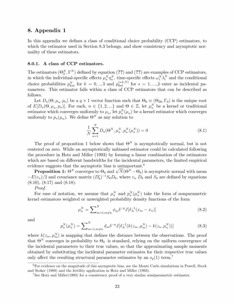
In this appendix we de�nes a class of conditional choice probability (CCP) estimators, towhich the estimator used in Section 8.3 belongs, and show consistency and asymptotic nor-mality of these estimators.

8.0.1. A class of CCP estimators.

The estimators (�N3 ;�N) de�ned by equation (??) and (??) are examples of CCP estimators,

in which the individual-speci�c e¤ects �Nn �Nn , time-speci�c e¤ects !

Nt �

Nt and the conditional

choice probabilities pNknt for k = 0; ::; 3 and p(s;k;N)0nt for s = 1; :::; � enter as incidental pa-rameters. This estimator falls within a class of CCP estimators that can be described asfollows.Let Dn(�; �n; pn) be a q � 1 vector function such that �0 � (�30;�0) is the unique root

of E[Dn(�; �n; pn)]: For each, n 2 f1; 2; :::g and � 2 �, let �Nn be a kernel or traditionalestimator which converges uniformly to �n, let p

Nn (�n) be a kernel estimator which converges

uniformly to pn(�n). We de�ne �N as any solution to

1

N

NXn=1

Dn(�N ; �Nn ; p

Nn (�

Nn )) = 0 (8.1)

The proof of proposition 1 below shows that �N is asymptotically normal, but is notcentered on zero. While an asymptotically unbiased estimator could be calculated followingthe procedure in Hotz and Miller (1993) by forming a linear combination of the estimatorswhich are based on di¤erent bandwidths for the incidental parameters, the limited empiricalevidence suggests that the asymptotic bias is unimportant.6

Proposition 1: �N converges to �0 andpN(�N��0) is asymptotic normal with mean

�E(vn)=2 and covariance matrix (D00)�1S0D0, where vn D0 and S0 are de�ned by equations

(8.10), (8.17) and (8.18).Proof.For ease of notation, we assume that �Nn and pNn (�

Nn ) take the form of nonparametric

kernel estimators weighted or unweighted probability density functions of the form

�Nn =XN

m=1;m 6=n�m�

�qJ [��1N (xm � xn)] (8.2)

andpNn (�

Nn ) =

XN

m=1;m6=ndm�

�qJ [��1N (k(zm; �Nm)� k(zn; �Nn ))] (8.3)

where k(zm; �Nm) is mapping that de�nes the distance between the observations. The proofthat �N converges in probability to �0 is standard, relying on the uniform convergence ofthe incidental parameters to their true values, so that the approximating sample momentsobtained by substituting the incidental parameter estimates for their respective true valuesonly a¤ect the resulting structural parameter estimates by an op(1) term.7

6For evidence on the magnitude of this asymptotic bias, see the Monte Carlo simulations in Powell, Stockand Stoker (1989) and the fertility application in Hotz and Miller (1993).

7See Hotz and Miller(1993) for a consistency proof of a very similar semiparametric estimator.

23

To establish the mean, covariance, and bias, we �rst consider an other estimator denotedby e�N , and show that this has the same asymptotic distributional properties as �N . Forease of notation, let Dn � Dn(�0; �n; pn), pn � pn(�n)

D0n ��@Dn(�0; �n; pn)

@�

�

D1n ��@Dn(�0; �n; pn)

@�n+@Dn(�0; �n; pn)

@pn:pn(�n)

@�n

�and

D2n ��@Dn(�0; �n; pn)

@pn

�The estimator e�N satis�es the equation

�N�1XN

n=1[Dn +D0n(e�N ��0)] (8.4)

= N�1XN

n=1[D1n(�

Nn � �n) +D2n(p

Nn (�

Nn )� pn(�n))] (8.5)

De�ne the quantities

vN1mn � D1n[�m��qJ [��1N (xm � xn)]� �n] +D1m[�n�

�qJ [��1N (xm � xn)]� �m] (8.6)

vN2mn � D2n[dm��qJ [��1N (k(zm; �

Nm)� k(zn; �Nn ))]� pn] (8.7)

+D2m[dn��qJ [��1N (k(zm; �

Nm)� k(zn; �Nn ))]� pm] (8.8)

vNmn � vN1mn + vN2mn (8.9)

vn = f(xn)[D1n(�n + �n) +D2n(pn + dn)]�D1n�n �D2npn (8.10)

where f(xn) is the density of xn:Expanding the �rst expression on the right-side of 8.4 using the de�nition of the non-

parametric estimator for �n yields

N�1XN

n=1[D1n(�

Nn � �n)

= N�1XN

n=1D1n[

XN

m=1;m 6=n�m�

�qJ [��1N (xm � xn)]� �n] (8.11)

= N�1XN

n=1

XN

m=1;m6=nD1n[�m�

�qJ [��1N (xm � xn)]� �n]

= N�1(N � 1)�1XN�1

n=1

XN

m=n+1vN1mn (8.12)

Similarly, the second expression on the right side of 8.4 may be written as

N�1XN

n=1D2n[p

Nn (�

Nn )� pn(�n)] = N�1(N � 1)�1

XN�1

n=1

XN

m=n+1vN2mn (8.13)

24

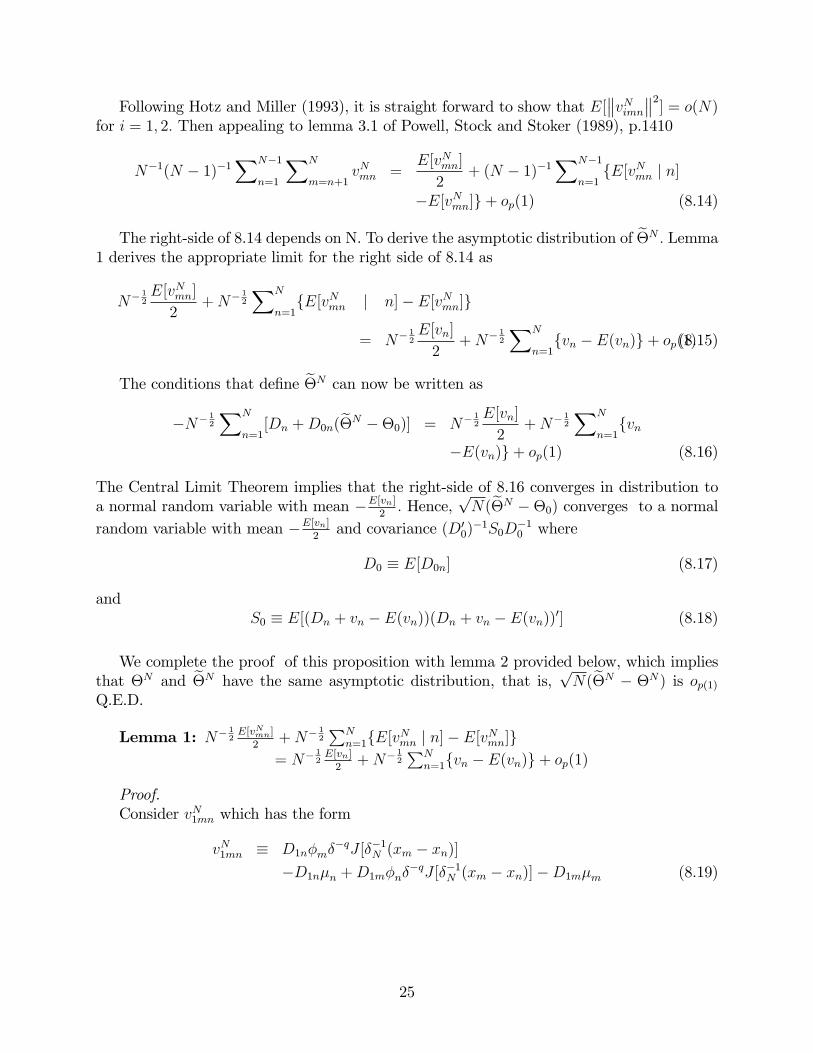
Following Hotz and Miller (1993), it is straight forward to show that E[ vNimn 2] = o(N)

for i = 1; 2: Then appealing to lemma 3.1 of Powell, Stock and Stoker (1989), p.1410

N�1(N � 1)�1XN�1

n=1

XN

m=n+1vNmn =

E[vNmn]

2+ (N � 1)�1

XN�1

n=1fE[vNmn j n]

�E[vNmn]g+ op(1) (8.14)

The right-side of 8.14 depends on N. To derive the asymptotic distribution of e�N : Lemma1 derives the appropriate limit for the right side of 8.14 as

N� 12E[vNmn]

2+N� 1

2

XN

n=1fE[vNmn j n]� E[vNmn]g

= N� 12E[vn]

2+N� 1

2

XN

n=1fvn � E(vn)g+ op(1)(8.15)

The conditions that de�ne e�N can now be written as�N� 1

2

XN

n=1[Dn +D0n(e�N ��0)] = N� 1

2E[vn]

2+N� 1

2

XN

n=1fvn

�E(vn)g+ op(1) (8.16)

The Central Limit Theorem implies that the right-side of 8.16 converges in distribution toa normal random variable with mean �E[vn]

2: Hence,

pN(e�N ��0) converges to a normal

random variable with mean �E[vn]2and covariance (D0

0)�1S0D

�10 where

D0 � E[D0n] (8.17)

andS0 � E[(Dn + vn � E(vn))(Dn + vn � E(vn))0] (8.18)

We complete the proof of this proposition with lemma 2 provided below, which impliesthat �N and e�N have the same asymptotic distribution, that is,

pN(e�N � �N) is op(1)

Q.E.D.

Lemma 1: N� 12E[vNmn]2

+N� 12

PNn=1fE[vNmn j n]� E[vNmn]g

= N� 12E[vn]2+N� 1

2

PNn=1fvn � E(vn)g+ op(1)

Proof.Consider vN1mn which has the form

vN1mn � D1n�m��qJ [��1N (xm � xn)]

�D1n�n +D1m�n��qJ [��1N (xm � xn)]�D1m�m (8.19)

25

Taking the �rst on the right-side of 8.19

E[D1n�m��qJ [��1(xm � xn)] j xn]

= D1n

Z�(x)��qJ [��1(x� xn)]f(x)dx

= D1n

Z�(xn + �u)J(u)f(xn + �u)du

=

ZD1nf�(xn)f(xn) + �(xn + �u)f(xn + �u)

��(xn)f(xn)gJ(u)du= D1n�(xn)f(xn) +D1ntn(�)

where tn(�) �R[�(xn + �u)f(xn + �u)� �(xn)f(xn)]J(u)du: Furthermore,

E[t(�)2] = E

(�2n

�Z[D1(xn + �u)f(xn + �u)�D1(xn)f(xn)]J(u)du

�2)

= E

(�2n

�Z xn+�u

xn

@(D1f)(x)

@xJ(u)du

�2)

� E

��2n

Z�2u2

@(D1f)(x)

@x

J(u)du�= E

��2n�

2

@(D1f)(x)

@x

�2u�= op(1):

Thus, tn(�) has a negligible e¤ect because its variance asymptotes to zero and it has a meanof zero. As a consequence,

N� 12

XN

n=1fE[D1n�m�

�qJ [��1(xm � xn)] j xn]

�E[D1n�m��qJ [��1(xm � xn)]]g

= N� 12

XN

n=1fD1n�nf(xn)

�E[D1n�nf(xn)]g+ op(1):Similarly, considering the third term in 8.4

N� 12

XN

n=1fE[D1m�n�

�qJ [��1(xm � xn)] j xn]

�E[D1m�n��qJ [��1(xm � xn)]]g

= N� 12

XN

n=1fD1nf(xn)�n

�E[D1nf(xn)�n]g+ op(1):It now follows that

N� 12

XN

n=1fE[vN1mn j n]� E[vN1mn]g

= N� 12

XN

n=1fD1nf(xn)(�n + �n)�D1n�n

�E[D1nf(xn)(�n + �n) +D1n�n] + op(1): (8.20)

26

By a similar argument

N� 12

XN

n=1fE[vN2mn j n]� E[vN2mn]g

= N� 12

XN

n=1fD2nf(xn)(pn + dn)�D2npn

�E[D2nf(xn)(pn + dn) +D2npn] + op(1): (8.21)

Q.E.D.

Lemma 2:pN(e�N ��N) is op(1):

Proof.Expanding the right-side of 8.1 about the true structural parameters, �0 and the true

incidental parameters, we obtain

� 1N

XN

n=1[Dn + eD0n(�

N ��0)]

=1

N

XN

n=1[ eD1n(�

Nn � �n) + eD2n(p

Nn (�

Nn )� pn(�n))] (8.22)

where ~ indicates that the appropriate partial derivatives are evaluated at points on theline segment joining (�0; �n; pn) and (�

N ; �Nn ; pNn ): Subtracting 8.22 from 8.4 gives

� 1N

XN

n=1[ eD0n(�0 ��N)�D0n(�0 � e�N)]

=1

N

XN

n=1[( eD1n �D1n)(�

Nn � �n)

+( eD2n �D2n)(pNn (�

Nn )� pn(�n))] (8.23)

consider the following asymptotic expansion

1

N

XN

n=1f eD0n(�0 ��N)�D0n(�0 � e�N)g

=1

N

XN

n=1fD0n(�0 ��N)�D0n(�0 � e�N) + ( eD0n �D0n)(�0 ��N)g

=1

N

XN

n=1D0n(e�N ��N) + op(1)(�0 ��N)

= fE[D0n] + op(1)g(e�N ��N) + op(1)(�0 ��N)= fE[D0n] + op(1)g(e�N ��N) + op(1) (8.24)

Considering the second expression in 8.23

1

N

XN

n=1[( eD1n �D1n)(�

Nn � �n) = op(1)

1

N

XN

n=1(�Nn � �n) (8.25)

where the right of 8.25 follows from the fact that eD1n converges in probability to D1n uni-formly in n: Similar U-statistic arguments to that used to justify the asymptotic normality ofpN(e�N��0), show that N� 1

2

PNn=1(�

Nn ��n) converges in distribution to a normal random

27

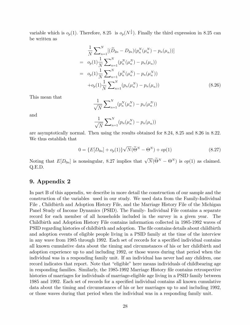
variable which is op(1): Therefore, 8.25 is op(N12 ): Finally the third expression in 8.25 can

be written as

1

N

XN

n=1[( eD2n �D2n)(p

Nn (�

Nn )� pn(�n))]

= op(1)1

N

XN

n=1(pNn (�

Nn )� pn(�n))

= op(1)1

N

XN

n=1(pNn (�

Nn )� pn(�Nn ))

+op(1)1

N

XN

n=1(pn(�

Nn )� pn(�n)) (8.26)

This mean that1pN

XN

n=1(pNn (�

Nn )� pn(�Nn ))

and1pN

XN

n=1(pn(�

Nn )� pn(�n))

are asymptotically normal. Then using the results obtained for 8.24, 8.25 and 8.26 in 8.22.We thus establish that

0 = fE[D0n] + op(1)gpN(e�N ��N) + op(1) (8.27)

Noting that E[D0n] is nonsingular, 8.27 implies thatpN(e�N � �N) is op(1) as claimed.

Q.E.D.

9. Appendix 2

In part B of this appendix, we describe in more detail the construction of our sample and theconstruction of the variables used in our study. We used data from the Family-IndividualFile , Childbirth and Adoption History File, and the Marriage History File of the MichiganPanel Study of Income Dynamics (PSID). The Family- Individual File contains a separaterecord for each member of all households included in the survey in a given year. TheChildbirth and Adoption History File contains information collected in 1985-1992 waves ofPSID regarding histories of childbirth and adoption. The �le contains details about childbirthand adoption events of eligible people living in a PSID family at the time of the interviewin any wave from 1985 through 1992. Each set of records for a speci�ed individual containsall known cumulative data about the timing and circumstances of his or her childbirth andadoption experience up to and including 1992, or those waves during that period when theindividual was in a responding family unit. If an individual has never had any children, onerecord indicates that report. Note that �eligible�here means individuals of childbearing agein responding families. Similarly, the 1985-1992 Marriage History �le contains retrospectivehistories of marriages for individuals of marriage-eligible age living in a PSID family between1985 and 1992. Each set of records for a speci�ed individual contains all known cumulativedata about the timing and circumstances of his or her marriages up to and including 1992,or those waves during that period when the individual was in a responding family unit.

28

Our sample selection started from the Childbirth and Adoption history �le, which con-tains 24,762 individuals. We initially selected women by setting �sex of individual�variableequal to two. Out of an initial sample of 24,762 individuals included in the Childbirth andAdoption �le, this initial selection produced a sample of 12,784 female. We then drop anyindividual who was in the survey for four years or less, this selection criteria eliminated afurther 1,946 individuals from our sample. We then drop all individuals who were older than45 in 1967, this eliminated an additional 1,531 individuals. We then drop all individualsthat were less than 14-years-old in 1991, this eliminated an additional 385 individuals.The corresponding number of observations for the interviewing year 1968 through 1992

are given by 5,429,5,608, 5,793,5,970, 6,197, 6,346, 6,510, 6,696, 6,876, 7,094, 7,236, 7,320,7,393, 7,455, 7,551, 7,634, 7,680, 7,761, 7,712, 7,666, 7,618, 7,574, 7,532, 7,378 and 7,233,respectively.Since individuals who had become non-respondents as of 1992, either because they and

their families were last to the study or they were mover-out non-respondents in years prior tothe 1992 interviewing year, are not in the twenty-�ve Family-Individuals Respondents File,the number of observations increases with the interviewing years.There were coding errors which occurred for the di¤erent measures of consumption in

the PSID from which we construct our consumption measure. In particular, our measure offood consumption expenditures for a given year is obtained by summing the values of annualfood expenditures for meals at home, annual food expenditures for eating out, and the valueof food stamps received for the year. We measured consumption expenditures for year t bytaking 0:25 of the value of this variable for the year t � 1 and 0:75 of its value for the yeart. The second step was taken to account for the fact that the survey questions used to elicitinformation about household food consumption is asked sometime in the �rst half of theyear, while the response is dated in the previous year.The variables used in the construction of the measure for total expenditures are also

subject to the problem of truncation from above in the way they are coded in the 1983PSID data tapes. The truncation value for the value of food stamps received for that year is$999.00, while the relevant value for this variable in the subsequent years and for the valueof food consumed at home and eating out is $9,999.00. Taken by itself, the truncation ofdi¤erent consumption variables resulted in a loss of 467 person-years. We also use variablesdescribing various demographic characteristics of the women in our sample. The dates ofbirth of the women were obtained from the Child Birth and Adoption �le. The age variableresulted in a loss of 162 individuals.The race of the individual or the region where they are currently residing were obtained

from the Family portion of the data record. We de�ned the region variable to be the geo-graphical region in which the household resided at the time of the annual interview. Thisvariable is not coded consistently across the years. For 1968 and 1969, the values 1 to 4denote the regions Northeast, Northcentral, South and West. For 1970 and 1971, the values5 and 6 denote the regions Alaska and Hawaii, and foreign country, respectively. After 1971a value of 9 indicates missing data but no person years were lost due to missing data forthese variables.We used the family variable �Race of The Household Head�to measure the race variable

in our study. For the interviewing years 1968-1970, the values 1 to 3 denote White, black, andPuerto Rican or Mexican, respectively. 7 denotes other (including Oriental and Philippino),

29

and 9 denotes missing data. For 1971 and 1972, the third category is rede�ned as Spanish-American or Cuban and between 1973-1984, just Spanish American. After 1984, the variablewas coded in such a way that 1-6 correspond to the categories White, Black, American Indian,Aleutian or Eskimo, and Asian or Paci�c Islander, respectively. A value of 7 denotes theother category, a value of 9 denotes missing. We used all available information for all theyears to assign the race of the individual for years in the sample when that information wasavailable.We used a combination of individual and family level variables to construct our measure

of educational attainment. This was because the variable for the individual does not containdata for the head of the household or wife, this we obtained from the family level �les.The marital status of a women in our subsample was determined by using the marriage

history �le. The number of individuals in the household and the total number of childrenwithin that household were also determined from the family level variables of the samename. In 1968, a code for missing data (equal to 99) was allowed for the �rst variable, butin the other years, missing data were assigned. The second variable was truncated above thevalue of 9 for the interviewing years 1968 and 1971. After 1975, this variable denotes theactual number of Children within the family unit.We constructed some additional variables. The variable showing the value of home-

ownership was constructed by multiplying the value of a household�s home by an indicatorvariable determining home ownership. A similar procedure was followed to generate value ofrent paid and rental value of free housing for a household. Mortgage payment and Principalof Mortgage outstanding were obtained from the family variables of the same names. Finally,household income was measured from the PSID variable total family money income, whichincluded taxable income of head and wife total transfer of head and wife, taxable income ofothers in the family units and their total transfer payments.We used two di¤erent de�ators to convert such nominal quantities as average hourly

earnings, household income, and so on to real. First, we de�ned the (spot) price of foodconsumption to be the numeraire good at t in the theoretical section. We accordinglymeasured real food consumption expenditures and real wages as the ratio of the nominalconsumption expenditures and wages and the annual Chain-type price de�ator for foodconsumption expenditures published in table t.12 of the National Income and Products. Onthe other hand, we de�ated variables such as the nominal value of home ownership or nominalfamily income by the Chain-type price de�ator for total personal consumption expenditures.

30

TABLEI

MainSam

pleSummaryStatistics

(StandardDeviationisparenthesis)

Variable

1968

1969

1970

1971

1972

1973

1974

1975

1976

1977

1978

1979

1980

Age

18.57

19.25

19.77

20.31

20.82

21.36

21.91

22.41

22.91

23.31

24.31

25.31

26.31

(12.59)

(12.67)

(12.81)

(13.01)

(13.17)

(13.33)

(13.51)

(13.72)

(13.93)

(14.19)

(14.19)

(14.19)

(14.19)

Education

11.31

11.30

11.27

11.25

11.22

11.20

11.18

11.14

11.13

11.13

11.13

11.13

11.13

(2.31)

(2.31)

(2.30)

(2.30)

(2.29)

(2.28)

(2.28)

(2.25)

(2.25)

(2.22)

(2.22)

(2.22)

(2.22)

FamilySize

5.78

5.67

5.49

5.36

5.23

4.98

4.81

4.65

4.52

4.42

4.31

4.15

4.05

(2.62)

(2.66)

(2.66)

(2.63)

(2.61)

(2.45)

(2.38)

(2.29)

(2.22)

(2.15)

(2.05)

(1.95)

(1.90)

YoungKids

1.61

1.54

1.45

1.38

1.31

1.26

1.20

1.14

1.08

1.02

0.97

0.93

0.88

(1.46)

(1.43)

(1.40)

(1.37)

(1.34)

(1.32)

(1.309)

(1.28)

(1.25)

(1.23)

(1.20)

(1.18)

(1.15)

OldKids

0.50

0.49

0.48

0.47

0.46

0.44

0.42

0.39

0.37

0.36

0.35

0.35

0.35

(1.13)

(1.12)

(1.09)

(1.08)

(1.04)

(0.99)

(0.94)

(0.90)

(0.85)

(0.81)

(0.79)

(0.75)

(0.74)

Birth

4.88

5.08

5.42

5.17

4.98

4.91

4.79

4.95

5.03

5.22

4.92

5.47

5.49

(21.55)

(21.97)

(22.64)

(22.14)

(21.74)

(21.61)

(21.36)

(21.68)

(21.86)

(22.25)

(21.64)

(22.75)

(22.78)

Ageat1stBirth

28.82

28.81

28.88

28.86

28.90

29.00

29.05

29.15

29.19

29.22

29.22

29.22

29.22

(11.31)

(11.31)

(11.33)

(11.34)

(11.36)

(11.39)

(11.41)

(11.43)

(11.44)

(11.44)

(11.44)

(11.44)

(11.44)

Martialstatus

23.11

24.51

25.65

27.01

28.59

30.13

31.33

31.95

32.66

33.73

34.35

35.80

36.73

(42.16)

(43.02)

(43.68)

(44.40)

(45.19)

(45.88)

(46.39)

(46.63)

(46.90)

(47.28)

(47.49)

(47.95)

(48.21)

Black

43.06

42.93

42.76

42.70

42.26

42.19

41.91

41.69

41.65

41.47

41.47

41.48

41.48

(49.52)

(49.50)

(49.48)

(49.47)

(49.40)

(49.39)

(49.35)

(49.31)

(49.30)

(49.27)

(49.27)

(49.28)

(49.27)

Hispanic

0.43

0.43

0.43

0.43

0.43

0.43

0.44

0.44

0.44

0.44

0.44

0.44

0.44

(2.03)

(2.04)

(2.03)

(2.03)

(2.04)

(2.03)

(2.05)

(2.06)

(2.05)

(2.05)

(2.05)

(2.05)

(2.05)

NorthEast

16.65

16.44

16.63

16.60

16.53

16.61

16.43

16.18

16.04

15.97

15.86

15.37

15.13

(37.26)

(37.07)

(37.24)

(37.21)

(37.15)

(37.22)

(37.06)

(36.83)

(36.70)

(36.63)

(36.53)

(36.07)

(35.84)

NorthCentral

24.58

24.78

24.50

24.55

24.75

24.703

24.26

24.20

24.06

23.82

23.68

23.45

23.56

(43.06)

(43.18)

(43.02)

(43.04)

(43.16)

(43.13)

(42.87)

(42.83)

(42.75)

(42.60)

(42.51)

(42.38)

(42.44)

South

44.72

44.61

44.44

44.62

44.85

44.73

45.29

45.26

45.25

45.47

45.33

45.95

46.122

(49.73)

(49.71)

(49.70)

(49.71)

(49.74)

(49.731)

(49.78)

(49.78)

(49.78)

(49.79)

(49.79)

(49.84)

(49.85)

L.F.Participation

25.96

29.51

32.60

34.13

35.99

36.42

38.87

40.43

42.09

42.92

45.62

50.17

52.62

(43.85)

(45.61)

(46.88)

(47.42)

(48.00)

(48.12)

(48.75)

(49.08)

(49.37)

(49.50)

(49.81)

(50.00)

(49.94

HoursWorked

299

339

375

394

415

436

480

494

515

542

586

656

693

(641)

(670)

(697)

(706)

(725)

(739)

(768)

(764)

(778)

(790)

(815)

(846)

(857)

Hourlyearnings

7.03

7.31

8.70

7.87

8.26

8.40

8.46

8.43

8.05

8.80

8.87

8.66

8.91

(5.93)

(5.56)

(27.50)

(6.98)

(7.83)

(7.22)

(7.29)

(9.26)

(6.67)

(10.39)

(10.59)

(8.00)

(8.01

FoodConsumption

7890

7577

7446

7464

7253

7704

7871

7323

7220

6665

6465

6546

63353

(3432)

(3312)

(3226)

(3321)

(3258)

(3271)

(3606)

(3303)

(3358)

(3202)

(3264)

(3270)

(3213)

Observations

4691

4859

5040

5206

5407

5580

5758

5946

6142

6356

6356

6357

6357

Note:L.F.isanabbreviationforlaborforce.Educationisyearsofcompletededucation.Youngkidsisthenumberchildrenlessthan6yearsold

andOldkidsisthenumberofchildrenbetweentheageof6and14.Foodconsumptionandhourlyearningsaremeasuredin1996dollars.Birth,

race,martialstatusandregionsismeasuredinpercentage.

2

TABLEI(Continued)

MainSam

pleSummaryStatistics

(StandardDeviationisparenthesis)

Variable

1981

1982

1983

1984

1985

1986

1987

1988

1989

1990

1991

1992

Age

27.31

28.30

29.30

30.21

31.15

32.13

33.10

34.09

35.06

36.03

37.01

38.03

(14.19)

(14.19)

(14.19)

(14.18)

(14.18)

(14.19)

(14.20)

(14.21)

(14.21)

(14.22)

(14.19)

(14.19)

Education

11.1312

11.13

11.13

11.13

11.13

11.136

11.13

11.14

11.14

11.15

11.15

11.16

(2.22)

(2.22)

(2.22)

(2.22)

(2.22)

(2.22)

(2.22)

(2.23)

(2.23)

(2.23)

(2.23)

(2.23)

FamilySize

3.97

3.87

3.79

3.72

3.63

3.56

3.48

3.42

3.37

3.30

3.25

3.17

(1.90)

(1.83)

(1.80)

(1.72)

(1.67)

(1.65)

(1.61)

(1.58)

(1.58)

(1.57)

(1.57)

(1.54)

YoungKids

0.84

0.79

0.74

0.68

0.64

0.58

0.53

0.49

0.44

0.39

0.34

0.29

(1.12)

(1.09)

(1.05)

(1.01)

(0.97)

(0.93)

(0.89)

(0.84)

(0.79)

(0.74)

(0.68)

(0.62)

OldKids

0.35

0.36

0.37

0.37

0.38

0.39

0.41

0.41

0.41

0.42

0.41

0.41

(0.73)

(0.73)

(0.73)

(0.74)

(0.75)

(0.75)

(0.76)

(0.77)

(0.77)

(0.77)

(0.76)

(0.77)

Birth

4.92

5.09

5.01

4.95

4.75

4.98

4.99

4.78

4.62

4.86

4.99

1.24

(21.64)

(21.99)

(21.83)

(21.70)

(21.28)

(21.76)

(21.78)

(21.35)

(20.99)

(21.5)

(21.78)

(11.08)

Ageat1stBirth

29.22

29.22

29.21

29.21

29.20

29.21

29.21

29.21

29.24

29.19

29.17

29.21

(11.44)

(11.44)

(11.43)

(11.43)

(11.42)

(11.42)

(11.42)

(11.41)

(11.40)

(11.39)

(11.38)

(11.39)

Martialstatus

37.28

38.05

39.11

40.11

40.91

41.31

41.68

42.35

43.04

43.55

43.68

43.75

(48.36)

(48.56)

(48.80

(49.01)

(49.17)

(49.24)

(49.31)

(49.41)

(49.51)

(49.58)

(49.60)

(49.61)

Black

41.48

41.48

41.48

41.28

41.22

41.22

40.97

40.79

40.61

40.46

40.31

40.05

(49.27)

(49.27)

(49.27)

(49.23)

(49.22)

(49.22)

(49.18)

(49.14)

(49.11)

(49.08)

(49.05)

(49.01)

Hispanic

0.44

0.44

0.44

0.44

0.44

0.44

0.43

0.43

0.43

0.43

0.43

0.44

(2.05)

(2.05)

(2.05)

(2.05)

(2.05)

(2.05)

(2.04)

(2.03)

(2.04)

(2.04)

(2.04)

(2.04)

NorthEast

14.96

14.77

14.48

14.38

14.18

14.09

13.92

13.69

13.50

13.08

12.75

12.54

(35.67)

(35.48)

(35.20)

(35.09)

(34.89)

(34.79)

(34.62)

(34.38)

(34.18)

(33.72)

(33.35)

(33.12)

NorthCentral

23.38

23.27

23.23

22.99

22.79

22.48

22.39

22.09

21.68

21.65

21.60

21.84

(42.33)

(42.26)

(42.23)

(42.08)

(41.95)

(41.75)

(41.69)

(41.48)

(41.21)

(41.19)

(41.15)

(41.32)

South

45.95

45.95

46.02

46.25

45.94

45.67

45.64

45.57

45.43

45.60

45.10

45.53

(49.84)

(49.84)

(49.84)

(49.86)

(49.83)

(49.81)

(49.81)

(49.80)

(49.79)

(49.81)

(49.76)

(49.80)

L.F.Particaption

54.47

55.01

55.85

57.74

61.75

62.71

64.57

67.01

68.32

70.76

72.13

71.47

(49.80)

(49.75)

(49.65)

(49.39)

(48.60)

(48.36)

(47.83)

(47.02)

(46.52)

(45.48)

(44.83)

(45.15)

HoursWorked

725

744

761

790

879

907

937

980

1017

1041

1077

1085

(866)

(875)

(883)

(889)

(915)

(929)

(927)

(938)

(947)

(937)

(946)

(962)

Hourlyearnings

8.73

8.65

8.67

10.78

9.88

9.93

9.58

9.97

10.11

10.42

10.33

10.57

(7.65)

(7.57)

(7.46)

(56.83)

(38.91)

(24.31)

(9.46)

(9.69)

(8.66)

(15.53)

(11.77)

(9.33)

FoodConsumption

6162

5886

5753

5875

5963

5846

5741

5766

5631

5518

5435

5512

(3118)

(2951)

(2966)

(3123)

(3707)

(3128)

(3105)

(2933)

(2835)

(3010)

(2834)

(3488)

Observations

6357

6357

6357

6298

6246

6159

6067

5971

5885

5815

5725

5627

Note:L.F.isanabbreviationforlaborforce.Note:Educationisyearsofcompletededucation.Youngkidsisthenumberchildrenlessthan6years

oldandOldkidsisthenumberofchildrenbetweentheageof6and14.Foodconsumptionandhourlyearningsaremeasuredin1996dollars.Birth,

race,martialstatusandregionsismeasuredinpercentage.

3

TABLE IIWage Equation

ln(wnt) = ln(ωt) + ln(µn) + z′ntB3 +

4∑s=1(δ1shn,t−s + δ2sd2n,t−s + δ2sd4n,t−s)

Variable Parameter Estimate†

Lags of hours worked

4hn,t−1 δ1114.1011(0.2337)

4hn,t−2 δ1210.9974(0.2471)

4hn,t−3 δ138.8360(0.2437)

4hn,t−4 δ145.4729(0.2227)

Lags of participation

4 (d2n,t−1 + d4n,t−1) δ21−6.8664

(4.01E − 02)4 (d2n,t−2 + d4n,t−2) δ22

−4.4241(4.46E − 02)

4 (d2n,t−3 + d4n,t−3) δ23−2.8986

(4.44E − 02)4 (d2n,t−4 + d4n,t−4) δ24

−1.6065(3.92E − 02)

Socioeconomic Variables

4AGE2nt B31−0.0114

(3.0E − 04)4(AGEnt × EDUnt) B32

0.0161(3.1E − 03)

† Estimated standard error in parenthesis. Note: EDU is the years of completed education.

4

TABLE IIILog Frisch Consumption Demand

ln(xnt) = (1− α)−1[z′ntB2 − ln(ηn)− ln(λt) + ε0nt]Variable Parameter Estimate†

Risk Aversion α0.98

(1.9E − 02

Socioeconomic variables

4FAMnt (1− α)−1B213.19E − 02(3.0E − 04)

4Y KIDnt (1− α)−1B22−3.33E − 02(1.6E − 03)

4OKIDnt (1− α)−1B23−1.12E − 02(1.2E − 03)

4AGE2nt (1− α)−1B24−1.0E − 04(0.0000)

Region Dummies

4NCnt (1− α)−1B25−3.7E − 03(3.3E − 03)

4SOnt (1− α)−1B26−1.19E − 02(3.2E − 03)

† Estimated standard error in parenthesis. Note: EDU is the years of completed education,FAM is the numberof individual in the household, YKid is the number of kids less than 6 years old, Okid is the number of childrenbetween age 6 and 14, while NC and SO are regional dummies for the North Central and South respectively.

5

TABLE IVFixed Utility from Labor Force Participation

(dnt2 + dnt4) z′ntB0

Variable Parameter Estimate†

CONSTANT B00−5.23(0.66)

AGEnt B010.26(4.6E − 2)

AGE2nt B02−4.8E − 3(7.46E − 4)

AGEnt × EDUCn B032.0E − 3(4.25E − 4)

MART.STATUSnt B040.12(4.9E − 2)

BLACKnt B05−5.9E − 2(5.2E − 2)

† Estimated standard error in parenthesis. Note: EDU is the years of completed education and MART.STATUS is a dummy variable equal 1 if the female is married and zero otherwise.

6

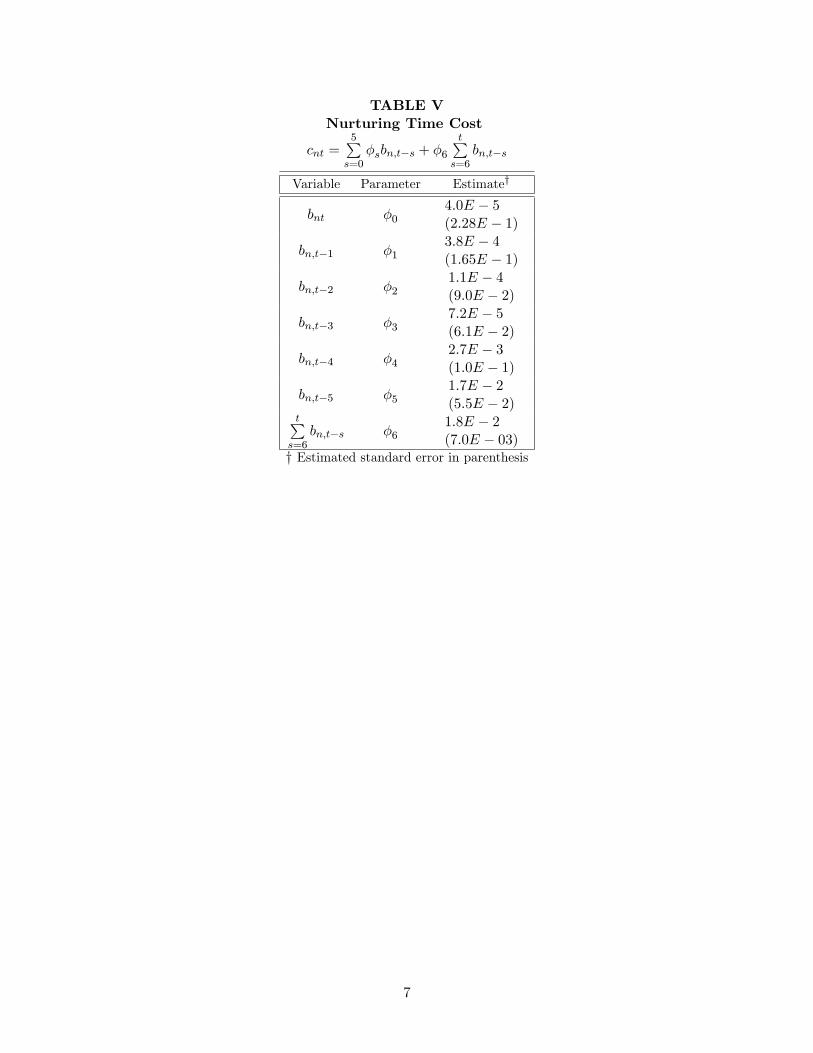
TABLE VNurturing Time Cost

cnt =5∑s=0

φsbn,t−s + φ6t∑s=6

bn,t−s

Variable Parameter Estimate†

bnt φ04.0E − 5(2.28E − 1)

bn,t−1 φ13.8E − 4(1.65E − 1)

bn,t−2 φ21.1E − 4(9.0E − 2)

bn,t−3 φ37.2E − 5(6.1E − 2)

bn,t−4 φ42.7E − 3(1.0E − 1)

bn,t−5 φ51.7E − 2(5.5E − 2)

t∑s=6

bn,t−s φ61.8E − 2(7.0E − 03)

† Estimated standard error in parenthesis

7

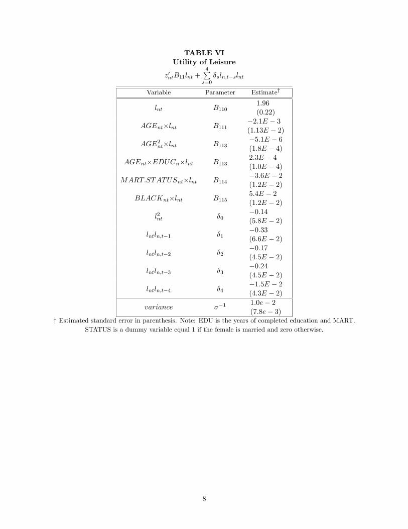
TABLE VIUtility of Leisure

z′ntB11lnt +4∑s=0

δsln,t−slnt

Variable Parameter Estimate†

lnt B1101.96(0.22)

AGEnt×lnt B111−2.1E − 3(1.13E − 2)

AGE2nt×lnt B113−5.1E − 6(1.8E − 4)

AGEnt×EDUCn×lnt B1132.3E − 4(1.0E − 4)

MART.STATUSnt×lnt B114−3.6E − 2(1.2E − 2)

BLACKnt×lnt B1155.4E − 2(1.2E − 2)

l2nt δ0−0.14(5.8E − 2)

lntln,t−1 δ1−0.33(6.6E − 2)

lntln,t−2 δ2−0.17(4.5E − 2)

lntln,t−3 δ3−0.24(4.5E − 2)

lntln,t−4 δ4−1.5E − 2(4.3E − 2)

variance σ−11.0e− 2(7.8e− 3)

† Estimated standard error in parenthesis. Note: EDU is the years of completed education and MART.STATUS is a dummy variable equal 1 if the female is married and zero otherwise.

8

TABLE VIIUtility from Offspring and Monetary Costs

γ0bnt +5∑k=1

γkbntbn,t−k + γ6t∑

k=6

bntbn,t−k

z′ntπ1

Variable Parameter Estimate†

bnt γ0−1.17(0.30)

bntbn,t−1 γ1−0.23(0.08)

bntbn,t−2 γ20.79(0.12)

bntbn,t−3 γ30.41(0.08)

bntbn,t−4 γ4−0.14(7.5E − 2)

bntbn,t−5 γ5−0.22(0.08)

t∑k=6

bntbn,t−k γ6−0.41(0.05)

NO HIGH SCHnt π1−5.1E − 3(0.13)

BLACKnt π21.6E − 2(8.4E − 2)

† Estimated standard error in parenthesis. Note: NO HIGH SCH is dummy variable equal one if the femalehas not graduated high school and zero otherwise.

9

TABLE VIIIPredicted Completed Fertility Outcomes under Different Policies

Marital Education Actual Estimation Expenses Daycare Wages Retraining

BlackM < 2.12 2.45 2.63 2.41 2.57 2.69

HS 1.93 2.03 2.60 2.8 2.19 3.00> 1.35 1.68 1.71 2.3 1.66 2.50

U < 2.15 2.35 2.56 2.58 2.41 2.57HS 1.82 1.97 2.04 2.1 1.98 2.05> 1.23 1.17 1.26 1.85 1.37 2.24

HispanicM < 2.08 2.19 2.23 2.31 2.25 2.02

HS 1.83 1.79 1.89 2.03 1.87 2.35> 1.55 1.46 1.50 1.87 1.49 2.03

U < 2.00 2.15 2.23 2.26 2.23 2.31HS 1.78 1.87 1.96 2.12 1.89 2.38> 1.46 1.56 1.67 2.00 1.72 2.30

WhiteM < 1.78 2.04 2.12 2.16 2.09 2.07

HS 1.34 1.52 1.63 2.30 1.67 2.45> 1.12 1.23 1.32 1.97 1.24 2.03

U < 1.47 1.56 1.54 1.78 1.58 1.87HS 1.25 1.31 1.56 1.90 1.67 2.08> 1.11 1.24 1.39 1.78 1.48 2.03

10

TABLE VIII(Percentage Change)Predicted Completed Fertility Outcomes under Different Policies

Percentage Change of EstmationMarital Education Actual Estimation Expenses Daycare Wages Retraining

BlackM < 2.12 2.45 7.35 -1.63 4.90 9.80

HS 1.93 2.03 28.08 37.93 7.88 47.78> 1.35 1.68 1.79 36.90 -1.19 48.81

U < 2.15 2.35 8.94 9.79 2.55 9.36HS 1.82 1.97 3.55 6.60 0.51 4.06> 1.23 1.17 7.69 58.12 17.09 91.45

HispanicM < 2.08 2.19 1.83 5.48 2.74 -7.76

HS 1.83 1.79 5.59 13.41 4.47 31.28> 1.55 1.46 2.74 28.08 2.05 39.04

U < 2 2.15 3.72 5.12 3.72 7.44HS 1.78 1.87 4.81 13.37 1.07 27.27> 1.46 1.56 7.05 28.21 10.26 47.44

WhiteM < 1.78 2.04 3.92 5.88 2.45 1.47

HS 1.34 1.52 7.24 51.32 9.87 61.18> 1.12 1.23 7.32 60.16 0.81 65.04

U < 1.47 1.56 -1.28 14.10 1.28 19.87HS 1.25 1.31 19.08 45.04 27.48 58.78> 1.11 1.24 12.10 43.55 19.35 63.71

11

TABLE IXPredicted Annual Labor Force Participation Rates under Different Policies

Marital Education Actual Estimation Expenses Daycare Wages Retraining

BlackM < 0.570 0.452 0.436 0.421 0.476 0.423

HS 0.673 0.772 0.722 0.732 0.724 0.723> 0.781 0.729 0.745 .742 0.732 0.732

U < 0.678 0.616 0.606 0.627 0.601 0.591HS 0.723 0.763 0.751 0.749 0.761 0.763> 0.897 0.912 0.913 0.916 0.915 0.921

HispanicM < 0.612 0.634 0.632 0.625 0.623 0.618

HS 0.722 0.745 0.739 0.738 0.737 0.735> 0.823 0.856 0.842 0.845 0.835 0.812

U < 0.732 0.742 0.692 0.693 0.695 0.683HS 0.752 0.765 0.745 0.746 0.748 0.746> 0.824 0.878 0.867 0.857 0.856 0.872

WhiteM < 0.678 0.693 0.687 0.598 0.662 0.597

HS 0.897 0.876 0.874 0.873 0.878 0.871> 0.912 0.927 0.921 0.928 0.926 0.923

U < 0.753 0.734 0.727 0.714 0.701 0.692HS 0.857 0.876 0.767 0.798 0.845 0.855> 0.866 0.857 0.867 0.849 0.867 0.856

12

TABLE IX(Percentage Change)Predicted Annual Labor Force Participation Rates under Different Policies

Percentage Change of EstmationMarital Education Actual Estimation Expenses Daycare Wages Retraining

BlackM < 0.57 0.452 -3.54 -6.86 5.31 -6.42

HS 0.673 0.772 -6.48 -5.18 -6.22 -6.35> 0.781 0.729 2.19 1.78 0.41 0.41

U < 0.678 0.616 -1.62 1.79 -2.44 -4.06HS 0.723 0.763 -1.57 -1.83 -0.26 0.00> 0.897 0.912 0.11 0.44 0.33 0.99

HispanicM < 0.612 0.634 -0.32 -1.42 -1.74 -2.52

HS 0.722 0.745 -0.81 -0.94 -1.07 -1.34> 0.823 0.856 -1.64 -1.29 -2.45 -5.14

U < 0.732 0.742 -6.74 -6.60 -6.33 -7.95HS 0.752 0.765 -2.61 -2.48 -2.22 -2.48> 0.824 0.878 -1.25 -2.39 -2.51 -0.68

WhiteM < 0.678 0.693 -0.87 -13.71 -4.47 -13.85

HS 0.897 0.876 -0.23 -0.34 0.23 -0.57> 0.912 0.927 -0.65 0.11 -0.11 -0.43

U < 0.753 0.734 -0.95 -2.72 -4.50 -5.72HS 0.857 0.876 -12.44 -8.90 -3.54 -2.40> 0.866 0.857 1.17 -0.93 1.17 -0.12

13