lie symmetry methods for local volatility models · lie symmetry methods for local volatility...
TRANSCRIPT

QUANTITATIVE FINANCE RESEARCH CENTRE QUANTITATIVE F
INANCE RESEARCH CENTRE
QUANTITATIVE FINANCE RESEARCH CENTRE
Research Paper 377 September 2016
Lie Symmetry Methods for Local Volatility Models
Mark Craddock and Martino Grasselli
ISSN 1441-8010 www.qfrc.uts.edu.au

Lie Symmetry Methods for Local Volatility Models
Mark Craddock∗ Martino Grasselli†
September 6, 2016
Abstract
We investigate PDEs of the form ut = 12σ
2(t, x)uxx − g(x)u which are associatedwith the calculation of expectations for a large class of local volatility models. We findnontrivial symmetry groups that can be used to obtain standard integral transformsof fundamental solutions of the PDE. We detail explicit computations in the separablevolatility case when σ(t, x) = h(t)(α + βx + γx2), g = 0, corresponding to the so calledQuadratic Normal Volatility Model. We also consider choices of g for which we can obtainexact fundamental solutions that are also positive and continuous probability densities.
Key words: Lie symmetries, fundamental Solution, PDEs, Local Volatility Models,Normal Quadratic Volatility Model.
1 Introduction
A symmetry of a differential equation is a transformation that maps solutions to solutions.Continuous symmetries which have group properties are called Lie symmetries, since themeans for computing them were developed in the late nineteenth century by Sophus Lie. Amodern account of the theory can be found in Olver’s book, Olver (1993) and the books ofBluman, such as Bluman and Kumei (1989).
The applications of Lie symmetry groups are extensive. These range from epidemiologyto finance. Examples of these applications in stochastic analysis and finance may be foundin references such as Craddock and Lennox (2007), Craddock and Lennox (2009), Craddockand Platen (2004), Lennox (2011), Craddock (2009), Craddock and Lennox (2012), Baldeauxand Platen (2013), Goard (2011), Goard (2000), Goard and Mazur (2013), Andersen (2011),Lipton (2002), Zuhlsdorff (2002), Carr et al. (2006), Carr et al. (2013), Cordoni and Di Persio(2014), Grasselli (2016) and Itkin (2013). This list is by no means exhaustive.
∗School of Mathematical and Physical Sciences, University of Technology Sydney. (Australia). Email:[email protected].
†Department of Mathematics, University of Padova (Italy) and Leonard de Vinci Pole Universitaire, Re-search Center, Finance Group, 92 916 Paris La Defense (France). Email: [email protected]. Acknowl-edgments: we are grateful to Giulio Miglietta, Johanes Ruf, Josef Teichmann and the participants of theQuantitative Methods in Finance conference (Sydney, December 2015) and the London Mathematical FinanceSeminar (London, March 2016) for useful discussions and suggestions. The usual disclaimer applies.
1

The aim of this paper is to approach the classical local volatility models from the perspec-tive of Lie symmetry analysis of the associated backward PDEs. The concept of a symmetrygroup of a PDE was introduced by Sophus Lie in the 1880s, see the collection Lie (1912).Lie’s methods have recently been applied to problems in stochastic analysis by, among others,Craddock and Platen (2004), Craddock and Lennox (2007) and Craddock and Lennox (2009),who focused mainly on “generalized square root” models of the form
dXt = f(Xt)dt+Xγt dWt,
for some constant γ. These models have obvious financial interpretations.In this paper, we focus on (local) martingale models of the form
dXt = σ(t,Xt)dWt, (1)
together with the associated parabolic backward equation
∂tu =1
2σ2(t, x)∂xxu. (2)
Here and throughout ∂x = ∂∂x etc. For suitable choices of σ, this PDE has many symme-
tries. If we have at hand a Lie Group that leaves the PDE invariant, then we can apply it toany solution to get another solution. The key result for finding the Lie Groups admitted bythe PDE is Lie’s Theorem. For a PDE of order n, we write down the infinitesimal generator vof the symmetry and obtain its so called n-th prolongation prnv (see below). Lie’s Theoremsays that v generates a symmetry of the PDE
P (x,Dαu) = 0, x ∈ Ω ⊆ Rm, Dαu = ∂xα11 ···xαm
nu, α1 + · · ·+ αm ≤ n,
if and only if prnv[P (x,Dαu)] = 0 whenever P (x,Dαu) = 0. See Olver (1993), Chapter 2.This condition leads to an equation in a set of independent functions of the derivatives
of u. As the equation must be true for arbitrary values of these independent functions, theircoefficients must vanish, leading to a linear system of equations known as the DeterminingEquations. Once these equations are solved, one can find the corresponding Lie group ad-mitted by the PDE. For linear parabolic PDEs on the line, Craddock proved that it is alwayspossible to find a symmetry that maps a nonzero solution to a generalised Fourier or Laplacetransform of a fundamental solution, see Craddock and Dooley (2010). The question of un-der what conditions these fundamental solutions yield transition densities for the underlyingstochastic process was addressed in Craddock and Lennox (2009) and Craddock (2009).
In this paper we give sufficient conditions directly on σ for the existence of a Lie groupadmitted by the PDE (2). We compute symmetries which lead directly to a Fourier integraltransform of the fundamental solution of the backwards PDE.
In the special case where σ(t, x) = h(t)(α + βx + γx2) (i.e. with σ a separable functionwith a polynomial of degree two dependence on the state variable Xt) we exponentiate thegroup to explicitly find the symmetries of the equation by considering separately the cases oftwo distinct real roots, a single real root and two distinct complex roots. This local volatility
2

case corresponds to the so called Quadratic Normal Volatility model that has been investi-gated, among others, by Zuhlsdorff (2002), Andersen (2011) and Carr et al. (2013). For thismodel, we provide the explicit expression for the (positive) fundamental solution that are alsoprobability densities, thus giving an analytical counterpart to the probabilistic justificationof the tractability of this model presented in Carr et al. (2013).
For pricing, we have the following generic situation. Generally one can show, for exampleby arbitrage arguments, that the price u(S, t) for a derivative security on an underlyingS ∈ Ω ⊆ Rn, is given by a solution of the terminal value problem for the parabolic PDE
ut + Lu = 0, u(S, T ) = f(S), S ∈ Ω ⊆ Rn, t ∈ [0, T ]. (3)
One transforms this to the initial value problem
ut = Lu = 0, u(S, 0) = f(S), S ∈ Ω ⊆ Rn, t ∈ [0, T ], (4)
by letting t → T − t. Clearly we require a unique, continuous price. For hedging we alsorequire the existence of a certain number of derivatives. This amounts to asking under whichcircumstances the Cauchy problem (4) has a unique, smooth solution. There is extensiveliterature on the question of existence and uniqueness of solutions. We cannot survey it allhere, but Theorem 16 of Friedman (1964) tells us that if ut = Lu is uniformly parabolic, withsmooth coefficients having bounded first and second derivatives in Ω × [0, T ] then (4) has
a unique solution satisfying∫ T0
∫Rn |u(x, t)| exp (−k|x|2)dxdt < ∞ for some constant k > 0.
This solution will also be smooth if f is not too pathological. Generally speaking, we getnon-uniqueness for smooth solutions only when the initial data grows extremely rapidly. Thisis precisely the situation in the famous example of non-uniqueness for the heat equation thatwas constructed by Tychonoff Tychonoff (1935). Financial considerations typically rule outsuch pathological situations.
Thus for pricing, we require fundamental solutions that return smooth continuous solu-tions of the pricing PDE, given reasonable payoffs. In this paper we exhibit such fundamentalsolutions. It is also sometimes possible to obtain fundamental solutions that are not contin-uous and which return solutions that are discontinuous at some point, typically the origin.We rule out such solutions on the grounds that the price should depend continuously on theunderlying.
2 Lie Symmetries for PDEs
In this Section, we will give a short introduction to Lie Groups of transformations with aparticular focus on their applications to the solution of PDE’s. In this introduction we followclosely the presentation given in Bluman and Kumei (1989). Another standard reference forthis topic is Olver (2000). Then we will focus on the relations between symmetry analysisof PDE’s and transform of solutions of PDE’s as studied in Craddock and Platen (2004),Craddock and Lennox (2007) and Craddock and Lennox (2009).
3

2.1 Invariance of a Differential Equation
Let us consider now the second order PDE in two independent variables (x, t) of the form
F (x, t, u, ux, ut, uxx, uxt, utt) = 0. (5)
We work exclusively on a second order PDE in two independent variables since this is thesetting which interests us here. Of course the results we are about to discuss are valid forODE’s as well and for differential equations of any order in general.
We now give a definition that will be crucial in the following. The PDE (5) is said toadmit the Lie Group of transformations (Xϵ, Tϵ, Uϵ)ϵ, for ϵ > 0, if the family of solutions of(5) is an invariant family of surfaces for (Xϵ, Tϵ, Uϵ)ϵ.
In other words, this implies that if we have at hand a Lie Group G that leaves the PDEinvariant, then we can apply it to any solution to get another solution. If the solution westart from is itself an invariant surface, then by applying the Lie Group to it, we will end upwith the solution itself. Here the crucial concept is that the Lie Group must act on the spacewhere the solutions of the PDE lives, in our case the (x, t, u)-space.
We introduce a vector field
v = ξ(x, t, u)∂x + τ(x, t, u)∂t + ϕ(x, t, u)∂u, (6)
which is the infinitesimal generator of G. We can extend the action of G in a natural wayto act also on the derivatives of u up to second order, by essentially requiring that the chainrule holds. We call this the second prolongation of G and denote it by G(2). The generatorof G(2) is the second prolongation of v. This is given by (see e.g. Bluman and Kumei (1989)and Olver (1993)):
pr2v = v + ϕx ∂
∂ux+ ϕt ∂
∂ut+ ϕxx ∂
∂uxx+ ϕxt ∂
∂uxt+ ϕtt ∂
∂utt.
Expressions for ϕt etc are given by the prolongation formula given below.The main result due to Lie (see e.g. Bluman and Kumei (1989)) is that the PDE (5)
admits the Lie Group of transformations (Xϵ, Tϵ, Uϵ) if and only if
F (x, t, u, ux, ut, uxx, uxt, utt) = 0 → (G(2)F )(x, t, u, ux, ut, uxx, uxt, utt) = 0,
that is the surface F (x, t, u, ux, ut, uxx, uxt, utt) = 0 is invariant for the second prolongationG(2) of the group action G. We refer e.g. to Bluman and Kumei (1989) for the construction ofthe second prolongation for a group. At the level of vector fields, this leads to Lie’s Theoremwhich states that v generates a one parameter group of symmetries if and only if
pr2v[F (x, t, u, ux, ut, uxx, uxt, utt)] = 0
whenever F (x, t, u, ux, ut, uxx, uxt, utt) = 0.The coefficients ϕx, ϕt etc are given by the prolongation formula, first published by Olver
(1978).
ϕJj (x, u
(n)) = DJ
(ϕj −
p∑i=1
ξiuji)+
p∑i=1
ξiujJ,i, (7)
4

where uji =∂uj
∂xi, and ujJ,i =
∂ujJ∂xi
, and DJ is the total differentiation operator.
In practice, we use the variable names rather than the multi-indices in the exponents. Sowe write ϕxx rather than ϕ1,1. The coefficient functions ϕx and ϕt are
ϕx = Dx (ϕ− ξux − τut) + ξuxx + τuxt
=(ϕx + ϕuux − ξxux − ξuu
2x − ξuxx − τxut − τuuxut − τuxt
)+ ξuxx + τuxt
= ϕx + (ϕu − ξx)ux − ξuu2x − τxut − τuuxut.
Similarly, ϕt = Dt (ϕ− ξux − τut) + ξuxt + τutt, which leads to
ϕt = ϕt − ξtux + (ϕu − τt)ut − ξuuxut − τuu2t ,
and
ϕxx = Dxx (ϕ− ξux − τut) + ξuxxx + τuxxt
= ϕxx + (2ϕxu − ξxx)ux − τxxut + (ϕuu − 2ξxu)u2x − 2τxuuxut
− ξuuu3x − τuuu
2xut + (ϕu − 2ξx)uxx − 2τxuxt − 3ξuuxuxx
− τuutuxx − 2τuuxuxt.
The coefficients ϕxt and ϕtt can be obtained in the same manner, but we do not need themfor our calculations.
2.2 Symmetries and Fundamental Solutions
In a series of articles of increasing generality, Craddock and his coauthors studied the sym-metries of some Kolmogorov backward equations associated to a real diffusion. Namely,Craddock and Platen (2004) studied the equation
∂tu = x∂xxu+ f(x)∂xu, x ∈ R+
whereas Craddock and Lennox (2007) studied the equation
∂tu = σxγ∂xxu+ f(x)∂xu− µxru, x ∈ R
and Craddock and Lennox (2009) studied the equation
∂tu = σxγ∂xxu+ f(x)∂xu− g(x)u, x ∈ R. (8)
In Craddock and Dooley (2010), it was shown that if the PDE
ut = A(x, t)uxx +B(x, t)ux + C(x, t)u, (9)
has a four dimensional Lie algebra of symmetries, then there always exists a symmetry map-ping a nontrivial solution u to a generalised Laplace transform of a product of a fundamentalsolution and u. Dividing out by u yields the desired fundamental solution. If the symmetry
5
algebra is six dimensional, then we obtain a generalised Fourier type transform.
Lie proved that if a PDE of the form (9) has a six dimensional group of symmetries,then it may be transformed to the heat equation by an invertible change of variables. If thesymmetry group is four dimensional, then it can be reduced to the form
ut = uxx −A
x2u, A = 0, (10)
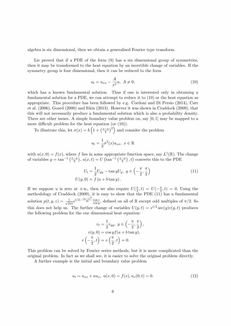
which has a known fundamental solution. Thus if one is interested only in obtaining afundamental solution for a PDE, we can attempt to reduce it to (10) or the heat equation asappropriate. This procedure has been followed by e.g. Cordoni and Di Persio (2014), Carret al. (2006), Goard (2000) and Itkin (2013). However it was shown in Craddock (2009), thatthis will not necessarily produce a fundamental solution which is also a probability density.There are other issues. A simple boundary value problem on, say [0, 1] may be mapped to amore difficult problem for the heat equation (or (10)).
To illustrate this, let σ(x) = b(1 +
(x−ab
)2)and consider the problem
ut =1
2σ2(x)uxx, x ∈ R
with u(x, 0) = f(x), where f lies in some appropriate function space, say L1(R). The changeof variables y = tan−1
(x−ab
), u(x, t) = U
(tan−1
(x−ab
), t)converts this to the PDE
Ut =1
2Uyy − tan yUy, y ∈
(−π
2,π
2
)(11)
U(y, 0) = f (a+ b tan y) .
If we suppose u is zero at ±∞, then we also require U(π2 , t) = U(−π2 , t) = 0. Using the
methodology of Craddock (2009), it is easy to show that the PDE (11) has a fundamental
solution p(t, y, z) = 1√2πt
et/2−(y−z)2
2tcos zcos y , defined on all of R except odd multiples of π/2. So
this does not help us. The further change of variables U(y, t) = et/2 sec(y)v(y, t) producesthe following problem for the one dimensional heat equation:
vt =1
2vyy, y ∈
(−π
2,π
2
),
v(y, 0) = cos yf(a+ b tan y),
v(−π
2, t)= v
(π2, t)= 0.
This problem can be solved by Fourier series methods, but it is more complicated than theoriginal problem. In fact as we shall see, it is easier to solve the original problem directly.
A further example is the initial and boundary value problem
ut = uxx + aux, u(x, 0) = f(x), ux(0, t) = 0. (12)
6

Solution of this problem yields the transition density for a reflected Brownian motion withdrift. This is a deceptively difficult problem as it cannot be solved by either the Fourier sineor cosine transform. Methods for its analytical solution can be found in Fokas (2008). Theyare however well outside the scope of this paper. It is possible to solve it using Lie symmetrymethods, similar to those presented here, but we will not do so here.
Here we observe that setting u(x, t) = e−ax/2−a2t/4v(x, t) reduces problem (12) to
vt = vxx, v(x, 0) = eax/2f(x), vx(0, t) =a
2ea
2t/4u(0, t).
So we have reduced the PDE to the heat equation, but the resulting boundary value problemcannot be solved as we do not know the value of u(0, t). The moral is that being able toreduce a PDE to the heat equation (or (10)) is not a universal panacea. We can arrive ata problem harder than the original, or indeed one that cannot be solved at all. Thereforeit is essential that we have techniques which yield solutions without the need to make anychanges of variables.
Note that the equation (8) corresponds to the backward Kolmogorov equations associatedto the diffusion which can be defined as a solution of the SDE
dXt = f(Xt)dt+√2σxγ/2dWt,
killed at the rate g(Xt). Thus if we define
v(x, t) = Ex
[e−
∫ t0 g(Xs)dsf(Xt)
],
then v is a solution of (8) with v(., 0) = f .If we take g = 0 in the argument above and f(x) = e−λx then we have
v(x, t) = Ex
[e−λXt
],
which is the Laplace transform of the marginal law of Xt. This Laplace transform can intheory be inverted, holding (x, t) fixed, to get the fundamental solution of the PDE whichcan be interpreted as the transition probability of the diffusion process.
The articles of Craddock and coauthors cited above sought to find solutions of the PDE’swith initial datum f(x) = e−λx by exploiting the symmetries of the PDE itself. Specifically,in the conservative case g = 0, they were able to find all the symmetries admitted by thePDE and then they noted that there is a symmetry that maps the solution constantly equalto 1 to a solution which is an exponential in x at t = 0. In the following section we willpursue a similar goal on an equation arising from a different linear diffusion.
3 The Problem
Following Bluman and Kumei (1989) and Olver (1993), we are looking for infinitesimal sym-metries of the PDE (2) when σ(t, x) = σ(x):
ut =1
2σ2(x)uxx − g(x)u, x ∈ D ⊆ R, σ > 0, (13)
7

where σ and g are functions defined in the state space domain D ⊂ R which we take to be aninterval of the form D = (xl;xr). As noted above, this is the Kolmogorov backward equationassociated to a diffusion X satisfying
dXt = σ(Xt)dWt, (14)
killed at rate g(Xt), where W is standard Brownian motion defined in a filtered probabilityspace (Ω,F , (Ft)t∈[0,T ],P).
Local Volatility Models typically include the presence of a time dependence in the volatil-ity, that is σ = σ(x, t). The special separable case
σ(x, t) = f(t)h(x), (15)
can be managed by the time-change methodology for the Brownian motion, see also Andersen(2011).
The general (not separable) case corresponding to (2) can be managed using the samemethodology, but it leads to extremely difficult equations. We prefer to leave this out sincelittle insight can be gained in those cases without a considerable amount of analysis.
Remark 3.1. If we specify a boundary condition like u(x, 0) = e−λx then, using a Feynman-Kac argument, (13) can be associated to the transform
u(x, t) = Ex
[exp
−λXt −
∫ t
0g(Xs)ds
].
The equation (13) can be transformed to one where the second derivative term has aconstant coefficient by introducing a change of variables. Let y =
∫ x dzσ(z) = b(x). We suppose
that b is invertible, so that x = b−1(y). Then set u(x, t) = U(b(x), t). Then
ux =1
σ(x)Uy, uxx =
1
σ2(x)Uyy −
σ′(x)
σ2(x)Uy,
so that (2) becomes
Ut =1
2Uyy −
1
2σ′(b−1(y))Uy − g(b−1(y))U. (16)
The more general equation
ut =1
2σ2(x)uxx + k(x)ux − g(x)u, (17)
can be transformed to
Ut =1
2Uyy +
(k(b−1(y))
σ(b−1(y))− 1
2σ′(b−1(y))
)Uy − g(b−1(y))U. (18)
Craddock and Lennox (2009) showed that a PDE of the form
ut = σxγuxx + f(x)ux − g(x)u,
8

has non-trivial symmetries if and only h(x) = x1−γf(x) satisfies an equation of the form
σxh′ − σh+1
2h2 + 2σx2−γg(x) = 2σAx2−γ +B (19)
σxh′ − σh+1
2h2 + 2σx2−γg(x) =
Ax4−2γ
2(2− γ)2+
Bx2−γ
2− γ+ C, (20)
σxh′ − σh+1
2h2 + 2σx2−γg(x) =
Ax4−2γ
2(2− γ)2+
Bx3−32γ
3− 32γ
+Cx2−γ
2− γ− κ, (21)
with κ = γ8 (γ − 4)σ2. See Craddock and Lennox (2009) for the specifics. We remark that
on the line, a non-trivial symmetry group will have dimensions of either four or six. Everytime homogeneous, linear parabolic PDE on the line has the trivial symmetries u(x, t) →cu(x, t + ϵ), which corresponds to a two dimensional symmetry group. A general resultdescribing conditions under which an arbitrary linear parabolic PDE on the real line has nontrivial symmetries follows easily.
Proposition 3.2. Let F (y) = y
(k(b−1(y))
σ(b−1(y))− 1
2σ′(b−1(y))
). Then the PDE (17) has non-
trivial symmetries if and only if
1
2yF ′ − 1
2F +
1
2F 2 + y2g(b−1(y)) = A1y
4 +B1y2 + C1y
3/2 +D1,
where y = b(x) =∫ x 1
σ(z)dz and the constants A1, ..., D1 are as in the right side of (19)-(21),with γ = 0.
This result is at the moment largely of theoretical interest. A more detailed account forhigher dimensional equations is in Vu’s forthcoming thesis, Vu (2016). For a given σ, we canobtain b and determine drift functions k for a given g such that the PDE has symmetriesand the results of Craddock (2009) can be employed to find fundamental solutions, if thesymmetry group is four dimensional. However, if we treat this as an equation for σ it is quitedifficult to deal with. So here we will derive an explicit equation for σ in the case of zerodrift and treat in detail a model which arises from this.
4 The Determining Equation
By applying the prolongation to the PDE (13) we get
pr2v
[ut −
1
2σ2uxx + gu
]= ϕt − σ(x)σ′(x)uxxξ −
1
2σ2(x)ϕxx + g′(x)uξ + g(x)ϕ,
which is
ϕt = σ(x)σ′(x)uxxξ +1
2σ2(x)ϕxx − g′(x)uξ − g(x)ϕ.
9

Since the PDE is linear, standard arguments (see e.g. Bluman and Kumei (1989)) implythat ξ and τ will be independent of u, that is
ξ = ξ(x, t), τ = τ(x, t),
and ϕ will be linear in u, that is ϕ(x, t, u) = αu + β for some α(x, t), β(x, t). Using thisinformation we obtain
βt + αtu+ (α− τt)ut − ξtux = σ(x)σ′(x)uxxξ − g′(x)uξ − g(x)(αu+ β)
+1
2σ2(x) (βxx + αxxu+ (2αx − ξxx)ux
−τxxut + (α− 2ξx)uxx − 2τxuxt) .
Let us now identify the coefficients of the last equation: the constant term gives
βt =1
2σ2(x)βxx − g(x)β,
which basically says that β satisfies the initial PDE. The coefficient of u yields
αt + τtg(x) =1
2σ2(x) (αxx + τxxg(x))− g′(x)ξ; (22)
while the coefficient of ux gives
−ξt =1
2σ2(x) (2αx − ξxx) . (23)
The coefficient of uxx gives
(α− τt)1
2σ2(x) = σ(x)σ′(x)ξ +
1
2σ2(x)
(−τxx
1
2σ2(x) + α− 2ξx
)(24)
and finally the coefficient of uxt gives2τx = 0, (25)
which implies τ = τ(t), so that (22) becomes
αt + τ ′(t)g(x) =1
2σ2(x)αxx − g′(x)ξ (26)
and from (24) we obtain
ξ(x, t) = σ(x)
(1
2τ ′(t)
∫ x 1
σ(y)dy + ρ(t)
), (27)
where ρ is an arbitrary deterministic function1. We now differentiate the last expression andwe plug the results into equation (23) that becomes
αx = − 1
σ2(x)ξt(x, t) +
1
2ξxx(x, t)
= −1
2τ ′′(t)
1
σ(x)
∫ x 1
σ(y)dy − ρ′(t)
1
σ(x)
+1
4τ ′(t)σ′′(x)
∫ x 1
σ(y)dy +
1
2ρ(t)σ′′(x) +
1
4τ ′(t)
σ′(x)
σ(x),
1We do not specify lower boundary of the integral since the constant term can be included into the arbitrarytime-dependent function ρ.
10

that we write in a more compact way by dropping the dependence on the arguments:
αx = −1
2τ ′′
1
σ
∫1
σ− ρ′
1
σ+
1
4τ ′σ′′
∫1
σ+
1
2ρσ′′ +
1
4τ ′σ′
σ. (28)
Integrating with respect to x gives
α = −1
4τ ′′(∫
1
σ
)2
− ρ′∫
1
σ+
1
4τ ′σ′
∫1
σ+
1
2ρσ′ + η, (29)
where η = η(t) is an arbitrary function of time. Also, differentiating (28) gives
αxx = −1
2τ ′′(− σ′
σ2
∫1
σ+
1
σ2
)+ ρ′
σ′
σ2+
1
2ρσ′′′ +
1
4τ ′(σ′′′∫
1
σ+ 2
σ′′
σ− (σ′)2
σ2
), (30)
and from (29) we get
αt = −1
4τ ′′′(∫
1
σ
)2
− ρ′′∫
1
σ+
1
4τ ′′σ′
∫1
σ+
1
2ρ′σ′ + η′. (31)
Then after some manipulations (26) becomes
−1
4τ ′′′(∫
1
σ
)2
− ρ′′∫
1
σ+ η′ = −1
4τ ′′ + ρ
(σ2
4σ′′′ − σg′
)+τ ′
[1
2
(σ2
4σ′′′ − σg′
)∫1
σ+
1
8
(2σσ′′ − (σ′)2
)− g
].
Now notice that1
8
(2σσ′′ − (σ′)2
)− g =
∫ (σ4σ′′′ − g′
)since
∫σ′′σ′ = (σ′)2/2, then we can write the determining equation granting the existence of
non trivial symmetries:
−1
4τ ′′′(∫
1
σ
)2
− ρ′′∫
1
σ+ η′ = −1
4τ ′′ + ρσ
(σ4σ′′′ − g′
)+τ ′
[σ
2
(σ4σ′′′ − g′
)∫ 1
σ+
∫ (σ4σ′′′ − g′
)]. (32)
Remark 4.1. The case σ(x) =√2x has been investigated by Craddock and Platen (2004),
who considered the following PDE
ut = xuxx + f(x)ux,
with D = R+. Taking g = 0 in (32) gives
−1
2xτ ′′′ −
√2xρ′′ +
τ ′′
4+ η′ =
3
16x32
√2ρ,
which agrees with Craddock and Platen (2004) p. 288 when (using their notation) we takef = 0; ρ =
√2ρ; σ′(t) = η′(t) + τ ′′(t)/4.
11

Remark 4.2. The case σ(x) =√2σxγ/2, γ = 2, has been investigated by Craddock and
Lennox (2007), who considered the following PDE
ut = σxγuxx + f(x)ux − µxru,
with D = R+, and subsequently by Craddock and Lennox (2009) in the more general case
ut = σxγuxx + f(x)ux − g(x)u.
In the latter case (32) gives
− x2−γ
2σ(2− γ)2τ ′′′ −
√2x1− γ
2
√σ(2− γ)
ρ′′ +τ ′′
4+ η′ = g′(x)ξ − τ ′(t)g(x) +
1
4ρσ
√2σγ
(γ2− 1)(γ
2− 2)x
32γ−3,
which agrees with formula (2.9) in Craddock and Lennox (2009) where we take f = 0; ρ =ρ√2σ.
From (32) we see that in order to match the terms depending on x we have to compare
the functional form of σ4σ
′′′ − g′ with the ones of(∫
1σ
)2and
∫1σ , or equivalently we have to
assume some functional forms for g. We then consider separately some cases.
5 The Infinitesimal Generators
In this section we show that if σ and g satisfy a given integro-differential equation, then thePDE (13) admits a symmetry group whose finite-dimensional part has dimension 6. In thefollowing theorem we state the requirement and find the associated determining equation(32). It is also possible to have Lie symmetry algebras which are two dimensional and fourdimensional. As we are interested in the quadratic local volatility model, for brevity, we willfocus on the six dimensional case.
Theorem 5.1. The PDE (13) admits a six dimensional Lie symmetry group if and only ifσ and g satisfy
1
4σσ′′′ − g′ = A
1
σ+B
1
σ
∫1
σ(33)
for some constants A,B ∈ R.
Proof. Under (33) the determining equation (32) becomes
−1
4τ ′′′(∫
1
σ
)2
− ρ′′∫
1
σ+ η′ = −1
4τ ′′ +Aρ+
(Bρ+
3
2Aτ ′)∫
1
σ+Bτ ′
(∫1
σ
)2
. (34)
Note that (34) involves only the expression∫ x
1/σ(y)dy which is a non constant function ofx. This allows us to identify the time-dependent coefficients and arrive to the system for τ ,ρ and η:
−1
4τ ′′′ = Bτ ′;
−ρ′′ = Bρ+3
2Aτ ′;
η′ = −1
4τ ′′ +Aρ.
12

Conversely, if σ, g do not satisfy (33), it follows immediately that either τ ′ = 0, whichin turns implies that there is no symmetry group transforming solutions which are constantin time to solutions which are not, see e.g. Baldeaux and Platen (2013) p. 129, or ρ = 0which will produce a four dimensional Lie symmetry algebra.2 The interested reader mayinvestigate this case.
In the following we compute the infinitesimal generator of the Lie group admitted by thePDE (13) in the case where B is null. The other cases can be treated similarly and we gatherthem in Appendix A.
Theorem 5.2. If σ and g satisfy (33) with B = 0 then the PDE
ut =1
2σ2(x)uxx − g(x)u, x ∈ D
admits a Lie symmetry group whose finite dimensional part has dimension 6. The corre-sponding Lie algebra is generated by the following infinitesimal symmetries:
v1 = σ(x)
(t
2
∫ x 1
σ(y)dy − A
4t3)∂x +
1
2t2∂t
+
(−1
4
(∫ x 1
σ(y)dy
)2
+
(3
4At2 +
t
4σ′(x)
)∫ x 1
σ(y)dy − σ′(x)
8At3 − t
4− 1
16A2t4
)u∂u;
v2 =
(σ(x)
2
∫ x 1
σ(y)dy − 3
8σ(x)At2
)∂x + t∂t
+
(3
4At
∫ x 1
σ(y)dy +
σ′(x)
4
∫ x 1
σ(y)dy − 3
16At2σ′(x)− 1
8A2t3
)u∂u;
v3 = ∂t;
v4 = σ(x)t∂x +
(−∫ x 1
σ(y)dy +
t
2σ′(x) +
1
2At2)u∂u;
v5 = σ(x)∂x +
(1
2σ′(x) +At
)u∂u;
v6 = u∂u.
All other symmetries of (13) have infinitesimal generators of the form vβ = β ∂∂u , where β is
an arbitrary solution of the PDE. These correspond to the superposition of symmetries. i.e.u → u+ β is a solution when u and β are solutions.
Remark 5.3. In the case g = A = 0 we recover σ′′′ = 0, corresponding to the QuadraticNormal Volatility Model. We will obtain fundamental solutions in this case below.
2The dimension of the Lie algebra is determined by the number of constants of integration. The functionρ appears as a second derivative, so it yields two constants of integration. If we set ρ = 0, we therefore reducethe dimension of the Lie algebra from six to four.
13

Proof. If B = 0, the system for τ , ρ and η admits the following solution:
τ(t) =C1
2t2 + C2t+ C3;
ρ(t) = −C1
4At3 − 3
8C2At
2 + C4t+ C5;
η(t) = −C1
16A2t4 − C2
8A2t3 +
C4
2At2 +
(C5A− C1
4
)t+ C6,
where C1, ..., C6 are arbitrary constants. From (27) we have
ξ(x, t) = σ(x)
(C1t+ C2
2
∫ x 1
σ(y)dy − A
4t3C1 −
3
8At2C2 + C4t+ C5
), (35)
and from (29) we get
α(x, t) = −C1
4
(∫ x 1
σ(y)dy
)2
−(−3
4C1At
2 − 3
4C2At+ C4
)∫ x 1
σ(y)dy
+1
4(C1t+ C2)σ
′(x)
∫ x 1
σ(y)dy +
1
2
(−C1
4At3 − 3
8C2At2 + C4t+ C5
)σ′(x)
−C1
16A2t4 − C2
8A2t3 +
C4
2At2 +
(C5A− C1
4
)t+ C6.
Recall that the latter equation for α determines ϕ as ϕ = αu+ β.We are looking for infinitesimal symmetries whose vector field has the following form:
v = ξ∂x + τ∂t + ϕ∂u,
then we arrive at
v = σ(x)
(C1t+ C2
2
∫ x 1
σ(y)dy − A
4t3C1 −
3
8At2C2 + C4t+ C5
)∂x
+
(1
2C1t
2 + C2t+ C3
)∂t
+
u
[−C1
4
(∫ x 1
σ(y)dy
)2
−(−3
4C1At
2 − 3
4C2At+ C4
)∫ x 1
σ(y)dy
+1
4(C1t+ C2)σ
′(x)
∫ x 1
σ(y)dy +
1
2
(−C1
4At3 − 3
8C2At2 + C4t+ C5
)σ′(x)
−C1
16A2t4 − C2
8A2t3 +
C4
2At2 +
(C5A− C1
4
)t+ C6
]+ β
∂u.
Now taking the coefficients of the arbitrary constants yields the result.
6 The Quadratic Normal Volatility Model
The preceding material provides the tools that are needed to obtain analytical results for awide class of models. Our aim now it to demonstrate how such an analysis can proceed, by
14

studying a well known case.
In this section we therefore consider the case B = 0, corresponding to 1/4σσ′′′−g′ = A/σ,in the specification where g = A = 0, which leads to
σ(x) = α+ βx+ γx2 (36)
with γ = 0 (the case γ = 0 corresponds to the so called shifted lognormal model). Thiscorresponds to the Quadratic Normal Volatility model, where the underlying process Xt
satisfies the following SDE:
dXt = (α+ βXt + γX2t )dWt,
that is a local volatility model deeply investigated in Lipton (2002), Zuhlsdorff (2002) andrecently re-discovered by Andersen (2011) and Carr et al. (2013). The Quadratic NormalVolatility model admits closed form formulas for the price of vanilla options and it is ingeneral highly tractable. The following subsections constitute an analytical counterpart ofthe probabilistic arguments of Carr et al. (2013) in support of the analytical tractability ofthe model. It admits indeed non trivial symmetries that are crucial in the determinationof the fundamental solutions to the PDE corresponding to the probability density of theunderlying.
6.1 Distinct Real Roots
We will consider here the case where the polynomial admits two distinct real roots l < m. Inthis case we can write w.l.o.g.
σ(x) =(x−m)(x− l)
m− l, m = l, (37)
corresponding to
dXt =(Xt −m)(Xt − l)
m− ldWt, X0 ∈ R.
Remark 6.1. The presence of a deterministic function f(t) such that
σ(x, t) = f(t)(x−m)(x− l)
m− l
can be managed by the time-change methodology for the Brownian motion, see (15).
This diffusion has the property that it will be absorbed when it hits either m or l, by theMarkov property.
In this case we have ∫ x 1
σ(y)dy = ln
x−m
x− l
and
σ′(x) =2x−m− l
m− l,
15

and we can exploit Theorem 5.2 to get the infinitesimal symmetries parametrized by the sixarbitrary coefficients C1, ..., C6:
v = ξ∂x + τ∂t + ϕ∂u
= C1
[t
2
(x−m)(x− l)
m− lln
x−m
x− l∂x +
1
2t2∂t
+
(−1
4ln2
x−m
x− l+
t
4
2x−m− l
m− lln
x−m
x− l− t
4− 1
2t2)u∂u
]+C2
[1
2
(x−m)(x− l)
m− lln
x−m
x− l∂x + t∂t +
1
4
2x−m− l
m− lln
x−m
x− lu∂u
]+C3∂t
+C4
[t(x−m)(x− l)
m− l∂x +
(− ln
x−m
x− l+
t
2
2x−m− l
m− l
)u∂u
]+C5
[(x−m)(x− l)
m− l∂x +
1
2
2x−m− l
m− lu∂u
]+C6u∂u,
together with the usual (infinite dimensional) symmetries generated byβu∂u.In order to obtain fundamental solutions we need useful symmetries. For the fundamental
solution on the line, we shall require a symmetry yielding a Fourier transform. To obtainsuch a symmetry we exponentiate v4.
Theorem 6.2. Consider the PDE
ut =1
2σ2(x)uxx, x ∈ D, (38)
with
σ(x) =(x−m)(x− l)
m− l
and D = R. Then the PDE (38) has a symmetry of the form
Uϵ(x, t) = u (fϵ(x, t), t) exp
−(ln
∣∣∣∣x−m
x− l
∣∣∣∣− t
2
)ϵ+
t
2ϵ2
1− x−mx−l e
−ϵt
1− x−mx−l
, (39)
where fϵ : D × R+ → R is defined by
fϵ(x, t) =m− l
(x−mx−l
)e−ϵt
1−(x−mx−l
)e−ϵt
.
That is, for ϵ sufficiently small , Uϵ is a solution of (38) whenever u is.
Proof. We take the symmetry v4 which is given by
v4 = t(x−m)(x− l)
m− l∂x +
(− ln
x−m
x− l+
t
2
2x−m− l
m− l
)u∂u,
16

and we exponentiate the symmetry, that is we look for the solution to the following system:
dx
dϵ= t
(x−m)(x− l)
m− l, x(0) = x;
dt
dϵ= 0, t(0) = t;
du
dϵ=
(− ln
∣∣∣∣ x−m
x− l
∣∣∣∣+ t
2
2x−m− l
m− l
)u, u(0) = u.
The solution of this system is given by
x−m
x− l=
x−m
x− leϵt (40)
t = t (41)
u = u exp
−(ln
∣∣∣∣x−m
x− l
∣∣∣∣− t
2
)ϵ− t
2ϵ2
1− x−mx−l
1− x−mx−l e
ϵt. (42)
Replacing the new parameters gives the result.
6.1.1 Obtaining Fundamental solutions
Fundamental solutions are not unique and with the methods we present here it is possibleto exhibit multiple fundamental solutions for certain PDEs. This is discussed in depth inCraddock and Lennox (2009). In this work we restrict ourselves to exhibiting fundamentalsolutions which are also positive and continuous probability densities.
We observe that the Lie algebras for our PDEs are all six dimensional, so we should lookfor a Fourier rather than a Laplace transform. This follows from a result in Craddock andDooley (2010). In the case of a four dimensional Lie algebra we look for a Laplace transformof a fundamental solution.
To obtain a Fourier transform we consider (39) and make the replacement ϵ → iϵ andtake u = 1. This gives
Uϵ(x, t) = exp
−(ln
∣∣∣∣x−m
x− l
∣∣∣∣− t
2
)iϵ− 1
2ϵ2t
1− x−m
x−l e−iϵt
1− x−mx−l
. (43)
At t = 0 we have
Uϵ(x, 0) = exp
(−iϵ ln
∣∣∣∣x−m
x− l
∣∣∣∣) .
Let us illustrate how we may find a fundamental solution with this solution. We supposethat x ∈ (l,m). In this case
ln
∣∣∣∣x−m
x− l
∣∣∣∣ = ln
(m− x
x− l
).
We seek a fundamental solution p such that∫ m
lexp
(−i ln
(m− y
y − l
)ϵ
)p(t, x, y)dy = exp
−(ln
(m− x
x− l
)− t
2
)iϵ− t
2ϵ2
1− x−mx−l e
−iϵt
1− x−mx−l
.
17

Observe that taking ϵ = 0 we get∫ m
lp(t, x, y)dy = U0 = 1,
so that p integrates to one and hence is a probability density.
Putting z = ln(m−yy−l
)and noting that dy = − ez(m−l)
(ez+1)2dz, we look for a fundamental
solution such that ∫ ∞
−∞e−izϵp(t, x, z)
ez(m− l)
(ez + 1)2dz = Uϵ(x, t).
Fourier inversion gives
p(t, x, z)ez(m− l)
(ez + 1)2=
1
2π
∫ ∞
−∞eiϵyUϵ(x, t)dϵ,
and this is a straightforward Gaussian integral. Inverting and making the appropriate sub-stitution back to the y variables gives the fundamental solution
p(t, x, y) =(m− l)(x− l)
(m−xx−l
) 1tln(
m−yy−l
)+ 1
2
√2πt(y − l)2(y −m)
exp
−
(2 ln
(m−yy−l
)+ t)2
+ 4 ln2(m−xx−l
)8t
,
(44)
for the equation (38) with l < x < m. Observe that for t > 0, limy→l,m p(t, x, y) = 0, so theapparent singularities at m, l are in fact zeroes. It is also clear that this fundamental solutionis positive and continuous.
Observe also that a solution given by
u(x, t) =
∫ m
lf(y)p(t, x, y)dy,
with p(t, x, y) given by (44), will satisfy the boundary conditions u(m, t) = u(l, t) = 0 whichcorresponds to the fact that these are absorbing points for the diffusion.
It is worth asking what happens if we take a different initial solution? There is no generalrule. For some PDEs we obtain another fundamental solution that is not a probability den-sity. In other cases we arrive back at the same fundamental solution that our first choice ofinitial solution produces. This first case is discussed extensively with examples in Craddockand Lennox (2009). The reader may check that taking the stationary solution u0(x) = x inthis case actually returns the same fundamental solution.
We can use the same symmetry to obtain other fundamental solutions. We illustrate byobtaining such a solution on (m,∞). We do so by obtaining a Fourier cosine transform.Taking the real part of (43) we see that
Vϵ(x, t) =exp
(−1
2ϵ2t)
m− l
[(x− l) cos
(ϵ
(g(x)− t
2
))+ (m− x) cos
(ϵ
(g(x) +
t
2
))],
18

with g(x) = ln(m−xl−x
), is also a solution of (38). Observe that Vϵ(x, 0) = cos
(ln(x−mx−l
)).
We look for a solution of (38) by setting∫ ∞
mcos
(ϵ ln
(y −m
y − l
))p(t, x, y)dy = Vϵ(x, t).
As before taking ϵ = 0 gives∫∞m p(t, x, y)dy = 1. Now the substitution z = − ln
(y−my−l
)produces the Fourier cosine transform∫ ∞
0cos(ϵz)p
(t, x,
mez − l
ez − 1
)(m− l)ez
(ez − 1)2dz = Vϵ(x, t).
We therefore have
p
(t, x,
mez − l
ez − 1
)(m− l)ez
(ez − 1)2=
2
π
∫ ∞
0cos(ϵz)Vϵ(x, t)dϵ.
Evaluating the inverse cosine transform and replacing with the original variables we arriveat the fundamental solution
p(t, x, y) =1√2πt
exp
−
(ln(y−my−l
)− t
2
)2+ ln2
(x−mx−l
)2t
K(t, x, y) (45)
in which
K(t, x, y) =
(m− l)(x− l)
(m−xl−x
) 2 ln(m−yy−l )t − 1
(x−mx−l
) 12−
ln( y−my−l )t
(y − l)(y −m)2.
It is not hard to see that limy→m p(t, x, y) = 0 and if
u(x, t) =
∫ ∞
mf(y)p(t, x, y)dy
then u(m, t) = 0. We may find other fundamental solutions for this case by these methods.For example we can obtain a fundamental solution on (−∞, l). However we shall leave thisto the interested reader.
Also, one could exponentiate symmetries generated by other vector fields and get differentfundamental solutions. In Appendix B we discuss this possibility by taking v1.
6.2 Single Real Root
We now consider the case where the polynomial admits one single root a of multiplicity 2.In this case we can write w.l.o.g.
σ(x) = (x− a)2, (46)
19

corresponding todXt = (Xt − a)2dWt, X0 ∈ R.
If we impose the initial condition X0 = a, then Xt = a is the unique solution of this SDEby the Yamada-Watanabe Theorem, see Klebaner (2005). Thus by the Markov property, ifXt reaches a, then it will remain at a. Of course one may condition the diffusion to be, sayreflected left or right at a, but we will not consider these cases here.
So we have ∫ x 1
σ(y)dy = − 1
x− a
andσ′(x) = 2(x− a),
and we can exploit theorem 5.2 again to get the infinitesimal symmetries parametrized bythe six arbitrary coefficients C1, ..., C6.
If we exponentiate v4 we have a symmetry that can be used to produce a fundamentalsolution.
Theorem 6.3. Consider the PDE
ut =1
2σ2(x)uxx, x ∈ D, (47)
withσ(x) = (x− a)2
and D = x ∈ R. Then the PDE (47) has a symmetry of the form
Uϵ(x, t) = u (fϵ(x, t), t) exp
1
x− aϵ+
t
2ϵ2(1 + (x− a)ϵt) , (48)
where fϵ : D × R+ → R is defined by
fϵ(x, t) =x− a
1 + (x− a)ϵt.
That is, for ϵ sufficiently small, Uϵ is a solution of (47) whenever u is.
Proof. We take the symmetry v4 which is given by
v4 = t(x− a)2∂x +
(1
x− a+ t(x− a)
)u∂u
and we exponentiate the symmetry, that is we look for the solution to the following system:
dx
dϵ= t(x− a)2, x(0) = x;
dt
dϵ= 0, t(0) = t;
du
dϵ=
(1
x− a+ t(x− a)
)u, u(0) = u.
20
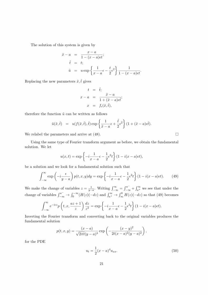
The solution of this system is given by
x− a =x− a
1− (x− a)ϵt;
t = t;
u = u exp
1
x− aϵ− t
2ϵ2
1
1− (x− a)ϵt.
Replacing the new parameters x, t gives
t = t;
x− a =x− a
1 + (x− a)ϵt;
x = fϵ(x, t),
therefore the function u can be written as follows
u(x, t) = u(f(x, t), t) exp
1
x− aϵ+
t
2ϵ2(1 + (x− a)ϵt).
We relabel the parameters and arrive at (48).
Using the same type of Fourier transform argument as before, we obtain the fundamentalsolution. We let
u(x, t) = exp
−i
1
x− aϵ− 1
2ϵ2t
(1− i(x− a)ϵt),
be a solution and we look for a fundamental solution such that∫ ∞
−∞exp
(−i
ϵ
y − a
)p(t, x, y)dy = exp
−i
1
x− aϵ− 1
2ϵ2t
(1− i(x− a)ϵt). (49)
We make the change of variables z = 1y−a . Writing
∫∞−∞ =
∫ a−
−∞+∫∞a+ we see that under the
change of variables∫ a−
−∞ →∫ −∞0 (H(z)(−dz) and
∫∞a+ →
∫ 0∞H(z)(−dz) so that (49) becomes∫ ∞
−∞e−iϵzp
(t, x,
az + 1
z
)dz
z2= exp
−i
1
x− aϵ− 1
2ϵ2t
(1− i(x− a)ϵt).
Inverting the Fourier transform and converting back to the original variables produces thefundamental solution
p(t, x, y) =(x− a)√
2πt(y − a)3exp
(− (x− y)2
2t(x− a)2(y − a)2
),
for the PDE
ut =1
2(x− a)4uxx. (50)
21

Taking ϵ = 0 in (49) shows that this fundamental solution is also a probability density,since the right side is equal to one at ϵ = 0 and the left is the integral of the fundamentalsolution. It is also not hard to check that taking the solution
u1(x, t) = exp
−i
1
x− aϵ− 1
2ϵ2t
(x− a),
leads to the same fundamental solution. Observe that a solution defined by
u(x, t) =
∫ ∞
−∞φ(y)
(x− a)√2πt(y − a)3
exp
(− (x− y)2
2t(x− a)2(y − a)2
)dy,
has the property u(a, t) = 0. So this density should correspond to a process which is absorbedat x = a, which is true of this process. One can also check that limy→a p(t, x, y) = 0. So wehave a positive fundamental solution, which is a continuous probability density.
Now let us study the process restricted to (a,∞). We do this by obtaining a Fourier cosinetransform. Taking the real part of (49) we see that
Uξ(x, t) = exp
(−ξ2t
2
)(cos
(ξ
x− a
)− ξt(x− a) sin
(ξ
x− a
))is a solution of (50). Observe that Uξ(x, 0) = cos
(ξ
x−a
). We therefore look for a solution
such that∫ ∞
acos
(ξ
y − a
)p(t, x, y)dy = exp
(−ξ2t
2
)(cos
(ξ
x− a
)− ξt(x− a) sin
(ξ
x− a
)).
Taking ξ = 0 gives∫∞a p(t, x, y)dy = 1, so such a fundamental solution will be a probability
density.Setting z = 1
y−a gives∫ ∞
0cos(ξz)p(t, x, 1/z + a)
dz
z2= exp
(−ξ2t
2
)(cos
(ξ
x− a
)− ξt(x− a) sin
(ξ
x− a
)).
This is a Fourier cosine transform. We can then recover the fundamental solution by
p(t, x, 1/z + a)/z2 =2
π
∫ ∞
0cos(ξz) exp
(−ξ2t
2
)(cos
(ξ
x− a
)− ξt(x− a) sin
(ξ
x− a
))dξ.
This leads to
p(t, x, y) =1√2πt
x− a
(y − a)2
[exp
((x+ y − 2a)2
2t(x− a)2(y − a)2
)− exp
((x− y)2
2t(x− a)2(y − a)2
)]× exp
(− 1
t(x− a)2− 1
t(y − a)2
).
A fundamental solution on (−∞, a) can also be obtained. We leave this to the interestedreader.
22

6.3 Distinct Complex Roots
We now consider the case where the polynomial admits two distinct complex roots a± ib andthe process starts at X0 ∈ R. In this case we can write without loss of generality
σ(x) = b
(1 +
(x− a
b
)2)
corresponding to
dXt = b
(1 +
(Xt − a
b
)2)dWt, X0 ∈ D,
with D = R. In this case we have∫ x 1
σ(y)dy = arctan
x− a
b
and
σ′(x) = 2x− a
b,
and we can exploit Theorem 6.3.2 again to get the infinitesimal symmetries parametrized bythe six arbitrary coefficients C1, ..., C6.
If we exponentiate v4 we have a symmetry that leads to the Fourier transform of afundamental solution, just as in the two distinct roots case.
Theorem 6.4. Consider the PDE
ut =1
2σ2(x)uxx, x ∈ D, (51)
with
σ(x) = b
(1 +
(x− a
b
)2)
and D = R. Then the PDE (51) has a symmetry of the form
Uϵ(x, t) = u (fϵ(x, t), t) exp
− arctan
(x− a
b
)ϵ+
t
2ϵ2
cos(arctan
(x−ab
)− ϵt
)cos(arctan
(x−ab
)) , (52)
where fϵ : D × R+ → R is defined by
fϵ(x, t) = a+ b tan
(arctan
(x− a
b
)− ϵt
).
That is, for ϵ sufficiently small, Uϵ is a solution of (51) whenever u is.
Proof. We take the non trivial symmetry associated to v4 which is given by
v4 = b
(1 +
(x− a
b
)2)t∂x +
(− arctan
(x− a
b
)+ t
x− a
b
)u∂u (53)
23

and we exponentiate the symmetry, that is we look for the solution to the followingsystem:
dx
dϵ= b
(1 +
(x− a
b
)2)t, x(0) = x;
dt
dϵ= 0, t(0) = t;
du
dϵ=
(− arctan
(x− a
b
)+ t
x− a
b
)u, u(0) = u.
The solution of this system is given by
x− a
b= tan
(arctan
(x− a
b
)+ ϵt
);
t = t;
u = u exp
− arctan
(x− a
b
)ϵ− t
2ϵ2
cos(arctan x−a
b
)cos(arctan x−a
b + ϵt) .
Replacing the new parameters x, t gives
t = t;x− a
b= tan(arctan
x− a
b− ϵt);
x = fϵ(x, t),
therefore the function u can be written as follows
u(x, t) =u(f(x, t), t) exp
− arctan
(x− a
b
)ϵ+
t
2ϵ2
cos(arctan x−a
b − ϵt)
cos(arctan x−a
b
) . (54)
We relabel the parameters and we arrive at (52).
6.3.1 A Fourier Series Representation of the Fundamental Solution
This case is interesting in that we actually obtain a Fourier series representation of ourfundamental solution, which is of course the Fourier transform on the circle. As this is asituation that has not been investigated previously in the literature, we will present thedetails.
From the previous symmetry we are able to exhibit the solution
u(x, t) =1
b
√(x− a)2 + b2e−
12ϵ2t−iϵ arctan(x−a
b ) cosh
(ϵt+ i arctan
(x− a
b
)), (55)
by taking our initial solution in equation (52) to be u = 1 and making the replacement ϵ → iϵ.We have
u(x, 0) = exp
(−iϵ arctan
(x− a
b
)). (56)
24

We therefore seek a fundamental solution p(t, x, y) such that∫ ∞
−∞u(y, 0)p(t, x, y)dy =
1
b
√(x− a)2 + b2e−
12ϵ2t−iϵ arctan(x−a
b ) cosh
(ϵt+ i arctan
(x− a
b
)).
(57)
It is clear from the fact U0 = 1 that this fundamental solutions satisfies∫∞−∞ p(t, x, y)dy = 1
and so is a probability density.We make the change of variables z = arctan
(y−ab
)and this becomes∫ π
2
−π2
e−iϵzp(t, x, a+ b tan z)sec2zdz =1
b2
√(x− a)2 + b2e−
12ϵ2t−iϵ arctan(x−a
b )
× cosh
(ϵt+ i arctan
(x− a
b
)).
Putting ϵ = 2n, z → z/2 leads to the expression
1
2π
∫ π
−πe−nizp(t, x, a+ b tan(z/2))sec2(z/2)dz =
1
b2π
√(x− a)2 + b2e−2n2t−2ni arctan(x−a
b )
× cosh
(2nt+ i arctan
(x− a
b
)),
which is the n-th Fourier coefficient of the kernel function. Fourier inversion then gives
p(t, x, a+ b tan(z/2)) =cos2(z/2)
b2π
∞∑n=−∞
eniz√
(x− a)2 + b2e−2n2t−2ni arctan(x−ab )
× cosh
(2nt+ i arctan
(x− a
b
)).
From this one easily obtains a Fourier series for the fundamental solution
p(t, x, y) =cos2
(arctan
(y−ab
))πb2
∞∑n=−∞
e2ni arctan(y−ab )√
(x− a)2 + b2e−2n2t
× e−2ni arctan(x−ab ) cosh
(2nt+ i arctan
(x− a
b
))=
1
π(a2 + (y − b)2)
∞∑n=−∞
e2ni arctan
(b(y−x)
1+(y−a)(x−a)
)e−2n2t
× [b cosh (2nt)− i(a− x) sinh(2nt)] .
7 Other tractable models
It is possible to obtain other models from this which are also tractable. In fact using ourmethods we can generate them quite easily. We consider the equation
1
4σσ′′′ − g′ = A
1
σ+B
1
σ
∫1
σ. (58)
25

Suppose we set A = B = 0 then integrate. This produces the nonlinear ODE
1
4σσ′′ − 1
8(σ′)2 − g = C, (59)
where C is a constant of integration. For specific choices of g this equation can be solved.For example, g(x) = µ/x implies that σ(x) = 4
√2µ/3
√x. And one can perform the analysis
we considered here in that case. However we can also reverse the process. If we specify σin equation (58) in advance and determine g from this. For this choice of g and σ we canthen compute appropriate fundamental solutions. Of course one might not have any specific
financial applications in mind for every functional E[exp
(−∫ t0 g(Xs)ds
)], but potentially
other useful models may be found in this way.
8 Conclusions
In this paper we gave conditions on σ for the tractability of a local volatility model and inthe special case of the Quadratic Normal Volatility model we were able to explicitly exponen-tiate the admitted Lie group of transformations to find the symmetries of the PDE and thecorresponding fundamental solutions. By doing so we provided an analytical counterpart tothe probabilistic justification of the tractability of this model given in Carr et al. (2013). Inthe future, we aim at finding symmetries of more general models (e.g. in the case where B isnot zero) and at inverting the resulting integral transforms to provide fundamental solutionsfor such models.
A Infinitesimal generator for B = 0
In this appendix we compute the infinitesimal generator of the Lie group admitted by thePDE (13) when the constant B in (33) is not null.
A.1 Case B > 0
Theorem A.1. If σ and g satisfy (33) with B > 0 then the PDE
ut =1
2σ2(x)uxx − g(x)u, x ∈ D
admits a Lie symmetry group whose finite dimensional part has dimension 6. The corre-sponding Lie algebra is generated by the following infinitesimal symmetries:
v1 = σ(x)
[−√B sin(2
√Bt)
∫ x 1
σ(y)dy − A√
Bsin(2
√Bt)
]∂x +
[cos(2
√Bt)]∂t
+
[B cos(2
√Bt)
(∫ x 1
σ(y)dy
)2
+ 2A cos(2√Bt)
∫ x 1
σ(y)dy
−√B
2sin(2
√Bt)σ′(x)
∫ x 1
σ(y)dy − A√
Bsin(2
√Bt)σ′(x)
+
√B
2sin(2
√Bt)− A2
2Bcos(2
√Bt)
]u∂u;
26
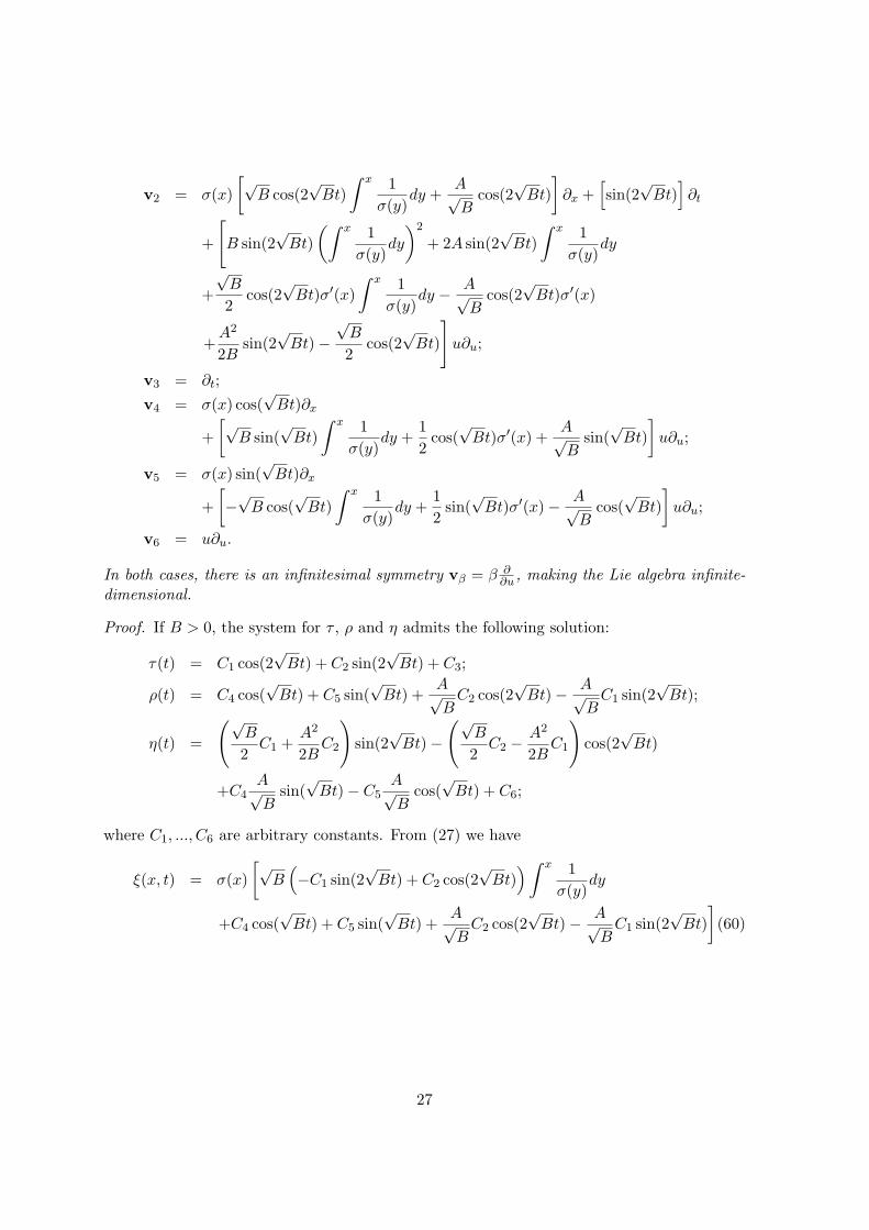
v2 = σ(x)
[√B cos(2
√Bt)
∫ x 1
σ(y)dy +
A√B
cos(2√Bt)
]∂x +
[sin(2
√Bt)]∂t
+
[B sin(2
√Bt)
(∫ x 1
σ(y)dy
)2
+ 2A sin(2√Bt)
∫ x 1
σ(y)dy
+
√B
2cos(2
√Bt)σ′(x)
∫ x 1
σ(y)dy − A√
Bcos(2
√Bt)σ′(x)
+A2
2Bsin(2
√Bt)−
√B
2cos(2
√Bt)
]u∂u;
v3 = ∂t;
v4 = σ(x) cos(√Bt)∂x
+
[√B sin(
√Bt)
∫ x 1
σ(y)dy +
1
2cos(
√Bt)σ′(x) +
A√B
sin(√Bt)
]u∂u;
v5 = σ(x) sin(√Bt)∂x
+
[−√B cos(
√Bt)
∫ x 1
σ(y)dy +
1
2sin(
√Bt)σ′(x)− A√
Bcos(
√Bt)
]u∂u;
v6 = u∂u.
In both cases, there is an infinitesimal symmetry vβ = β ∂∂u , making the Lie algebra infinite-
dimensional.
Proof. If B > 0, the system for τ , ρ and η admits the following solution:
τ(t) = C1 cos(2√Bt) + C2 sin(2
√Bt) + C3;
ρ(t) = C4 cos(√Bt) + C5 sin(
√Bt) +
A√BC2 cos(2
√Bt)− A√
BC1 sin(2
√Bt);
η(t) =
(√B
2C1 +
A2
2BC2
)sin(2
√Bt)−
(√B
2C2 −
A2
2BC1
)cos(2
√Bt)
+C4A√B
sin(√Bt)− C5
A√B
cos(√Bt) + C6;
where C1, ..., C6 are arbitrary constants. From (27) we have
ξ(x, t) = σ(x)
[√B(−C1 sin(2
√Bt) + C2 cos(2
√Bt))∫ x 1
σ(y)dy
+C4 cos(√Bt) + C5 sin(
√Bt) +
A√BC2 cos(2
√Bt)− A√
BC1 sin(2
√Bt)
](60)
27

and from (29) we get
α(x, t) = B(C1 cos(2
√Bt) + C2 sin(2
√Bt))(∫ x 1
σ(y)dy
)2
+(√
BC4 sin(√Bt)−
√BC5 cos(
√Bt) + 2AC2 sin(2
√Bt) + 2AC1 cos(2
√Bt))×∫ x 1
σ(y)dy +
√B
2
(−C1 sin(2
√Bt) + C2 cos(2
√Bt))σ′(x)
∫ x 1
σ(y)dy
+1
2
(C4 cos(
√Bt) + C5 sin(
√Bt) +
A√BC2 cos(2
√Bt)− A√
BC1 sin(2
√Bt)
)σ′(x)
+
(√B
2C1 +
A2
2BC2
)sin(2
√Bt)−
(√B
2C2 −
A2
2BC1
)cos(2
√Bt)
+C4A√B
sin(√Bt)− C5
A√B
cos(√Bt) + C6.
Now taking the coefficients of the arbitrary constants yields the result.
A.2 Case B < 0
Theorem A.2. If σ and g satisfy (33) with B < 0 then the PDE
ut =1
2σ2(x)uxx − g(x)u, x ∈ D
admits a Lie symmetry group whose finite dimensional part has dimension 6. The corre-sponding Lie algebra is generated by the following infinitesimal symmetries:
v1 = σ(x)
[−√B exp(−2
√−Bt)
∫ x 1
σ(y)dy +
A√−B
exp(−2√−Bt)
]∂x
+
[B exp(−2
√−Bt)
(∫ x 1
σ(y)dy
)2
+ 2A exp(−2√−Bt)
∫ x 1
σ(y)dy
−√−B
2exp(−2
√−Bt)σ′(x)
∫ x 1
σ(y)dy +
A√−B
exp(−2√−Bt)σ′(x)
+
(√−B
2+
A2
2B
)exp(−2
√−Bt)
]u∂u +
[exp(−2
√−Bt)
]∂t;
28

v2 = σ(x)
[√−B exp(2
√−Bt)
∫ x 1
σ(y)dy − A√
−Bexp(2
√−Bt)
]∂x
+
[B exp(2
√−Bt)
(∫ x 1
σ(y)dy
)2
− 2A exp(2√−Bt)
∫ x 1
σ(y)dy
+
√−B
2exp(2
√−Bt)σ′(x)
∫ x 1
σ(y)dy − A√
−Bexp(2
√−Bt)σ′(x)
−(√
−B
2− A2
2B
)exp(2
√−Bt)
]u∂u +
[exp(2
√−Bt)
]∂t;
v3 = ∂t;
v4 = σ(x) exp(−√−Bt)∂x +
[√−B exp(−
√−Bt)
∫ x 1
σ(y)dy +
1
2exp(−
√−Bt)σ′(x)
− A√−B
exp(−√−Bt)
]u∂u;
v5 = σ(x) exp(√−Bt)∂x +
[−√−B exp(
√−Bt)
∫ x 1
σ(y)dy +
1
2exp(
√−Bt)σ′(x)
+A√−B
exp(√−Bt)
]u∂u;
v6 = u∂u.
Proof. If B < 0, the system for τ , ρ and η admits the following solution:
τ(t) = C1 exp(−2√−Bt) + C2 exp(2
√−Bt) + C3;
ρ(t) = C4 exp(−√−Bt) + C5 exp(
√−Bt) +
A√−B
C1 exp(−2√−Bt)− A√
−BC2 exp(2
√−Bt);
η(t) =
(√−B
2+
A2
2B
)C1 exp(−2
√−Bt)−
(√−B
2− A2
2B
)C2 exp(2
√−Bt)
−C4A√−B
exp(−√−Bt) +
A√−B
C5 exp(√−Bt);
where C1, ..., C6 are arbitrary constants. From (27) we have
ξ(x, t) = σ(x)
[−√−B
(C1 exp(−2
√−Bt)− C2 exp(2
√−Bt)
)∫ x 1
σ(y)dy
+C4 exp(−√−Bt) + C5 exp(
√−Bt) +
A√−B
C1 exp(−2√−Bt)− A√
−BC2 exp(2
√−Bt)
],
29

and from (29) we get
α(x, t) = B(C1 exp(−2
√−Bt) + C2 exp(2
√−Bt)
)(∫ x 1
σ(y)dy
)2
+(√
−BC4 exp(−√−Bt)−
√−BC5 exp(
√−Bt)
+2AC1 exp(−2√−Bt)− 2AC2 exp(2
√−Bt)
)∫ x 1
σ(y)dy
−√−B
2
(C1 exp(−2
√−Bt)− C2 exp(2
√−Bt)
)σ′(x)
∫ x 1
σ(y)dy
+1
2
(C4 exp(−
√−Bt) + C5 exp(
√−Bt)
+A√−B
C1 exp(−2√−Bt)− A√
−BC2 exp(2
√−Bt)
)σ′(x)
+
(√−B
2+
A2
2B
)C1 exp(−2
√−Bt)−
(√−B
2− A2
2B
)C2 exp(2
√−Bt)
−C4A√−B
exp(−√−Bt) +
A√−B
C5 exp(√−Bt).
Now taking the coefficients of the arbitrary constants yields the result for the case B <0.
B Another symmetry in the distinct real roots case
In this appendix we analyze another symmetry for the PDE (38) starting from another vectorfield generating the Lie symmetry.
Theorem B.1. Consider the PDE (38) with D = x ∈ R : x > m > l. Then the PDE(38) has a symmetry of the form
Uϵ(x, t) =
(x−m)
((x−lx−m
) 11+4ϵt − 1
)(m− l)
√1 + 4ϵt
exp
−ϵ(2 log
(x−mx−l
)+ t)2
2(1 + 4ϵt)
u
(fϵ(x, t),
t
1 + 4ϵt
),
(61)
where fϵ : D × R+ → R is defined by
fϵ(x, t) =m− l
(x−mx−l
) 11+4ϵt
1−(x−mx−l
) 11+4ϵt
.
That is, for ϵ sufficiently small, Uϵ is a solution of (38) whenever u is.
30

Proof. We take the vector field by
v1 = 4t(x−m)(x− l)
m− lln
x−m
x− l∂x + 4t2∂t
+
(−1
2t2 − 2 ln2
x−m
x− l+ 2t
2x−m− l
m− lln
x−m
x− l− 2t
)u∂u
and we exponentiate the symmetry, that is we look for the solution to the following system:
dx
dϵ= 4t
(x−m)(x− l)
m− lln
x−m
x− l, x(0) = x; (62)
dt
dϵ= 4t2, t(0) = t; (63)
du
dϵ=
(−1
2t2 − 2 ln2
x−m
x− l+ 2t
2x−m− l
m− lln
x−m
x− l− 2t
)u, u(0) = u. (64)
The calculations are straightforward, though somewhat tedious.From (63) we immediately get
t =t
1− 4ϵt,
then (62) becomes
(m− l)dx
(x−m)(x− l) ln x−mx−l
=4t
1− 4ϵtdϵ, x(0) = x,
which through the change of variable y = (x−m)/(x− l) transforms into
dy
y ln y= −d ln(1− 4ϵt),
thus giving
x−m
x− l=
(x−m
x− l
) 11−4ϵt
.
Then (64) becomes
du
u=
−12 t
2
(1− 4ϵt)2− 2
(1− 4tϵ)2ln2
x−m
x− l+
2t
(1− 4tϵ)2
1 +(x−mx−l
) 11−4ϵt
1−(x−mx−l
) 11−4ϵt
lnx−m
x− l− 2t
1− 4tϵ
dϵ,
with u(0) = u. Integrating and relabeling the parameters completes the proof.
The symmetry can be extended in a straightforward way to values of x to the left of mby taking absolute values.
We can obtain a fundamental solution from this symmetry. The style of argument isessentially the same as in for example Craddock and Lennox (2007). If we look for a fun-damental solution on (m,∞) using this symmetry then we are lead to a Laplace transform,which yields the fundamental solution (45). We also leave this to the interested reader. Infact we will obtain the fundamental solution already obtained for the case x > m, so we donot pursue it here.
31

References
Andersen, L. (2011). Option pricing with quadratic volatility: a revisit. Finance and Stochas-tics, 15:191–219.
Baldeaux, J. and Platen, E. (2013). Functionals of Multidimensional Diffusions with Appli-cations to Finance. Bocconi & Springer Series, Vol. 5.
Bluman, G. and Kumei, S. (1989). Symmetry and Differential Equations. Springer, NewYork.
Carr, P., Fischer, T., and Ruf, J. (2013). Why are quadratic normal volatility models ana-lytically tractable? SIAM J. Financial Mathematics, 4:185–202.
Carr, P., Laurence, P., and Wang, T.-H. (2006). Generating integrable one dimensionaldriftless diffusions. C. R. Acad. Sci. Paris, 343:393–398.
Cordoni, F. and Di Persio, L. (2014). Lie symmetry approach to the CEVmodel. InternationalJournal of Differential Equations and Applications, 133:109–127.
Craddock, M. (2009). Fundamental Solutions, Transition Densities and the Integration of LieSymmetries. J. Differential Equations, 246(1):2538–2560.
Craddock, M. and Dooley, A. (2010). On the Equivalence of Lie Symmetries and GroupRepresentations. J. Differential Equations, 249(1):621–653.
Craddock, M. and Lennox, K. (2007). Lie group symmetries as integral transforms of funda-mental solutions. Journal of Differential Equations, 232:652–674.
Craddock, M. and Lennox, K. (2009). The Calculation of Expectations for Classes of DiffusionProcesses by Lie Symmetry Methods. Annals of Applied Probability, 19(1):127–157.
Craddock, M. and Lennox, K. (2012). Lie Symmetry Methods for Multidimensional ParabolicPDEs and Diffusions. J. Differential Equations, 252:56–90.
Craddock, M. and Platen, E. (2004). Symmetry Group Methods for Fundamental Solutions.Journal of Differential Equations, 207:285–302.
Fokas, A. (2008). A Unified Approach to Boundary Value Problems. Number 78 in RegionalConference Series in Applied Mathematics. SIAM, Philadelphia.
Friedman, A. (1964). Partial Differential Equations of Parabolic Type. Prentice Hall, Engle-wood Cliffs, NJ.
Goard, J. (2000). New Solutions to the Bond-Pricing Equation via Lie’s Classical Method.Mathematical and Computer Modelling, 32:299–313.
Goard, J. (2011). Pricing of volatility derivatives using 3/2-stochastic models. Proceedingsof the World Congress on Engineering 2011, 1:443–438.
32

Goard, J. and Mazur, M. (2013). Stochastic volatility models and the pricing of VIX options.Mathematical Finance, 23(3):139–158.
Grasselli, M. (2016). The 4/2 stochastic volatility model. Mathematical Finance, to appear.Available at http : //papers.ssrn.com/sol3/papers.cfm?abstractid = 2523635.
Itkin, A. (2013). New solvable stochastic volatility models for pricing volatility derivatives.Review of Derivatives Research, 16:111–134.
Klebaner, F. C. (2005). Introduction to Stochastic Calculus with Applications. ImperialCollege Press, London, 2 edition.
Lennox, K. (2011). Lie Symmetry Methods for Multi-dimensional Linear Parabolic PDEsand Diffusions. PhD Thesis, UTS, Sydney.
Lie, S. (1912). Vorlesungen uber Differentialgleichungen mit bekannten infinitesimalen Tran-formatioen. Teubner.
Lipton, A. (2002). The Vol Smile Problem. RISK, February:61–65.
Olver, P. (1978). Symmetry groups and conservation laws in the formal variational calculus.Working paper, University of Oxford.
Olver, P. J. (1993). Applications of Lie Groups to Differential Equations. Graduate Texts inMathematics, Springer, New York.
Tychonoff, A. (1935). Theoremes d’unicite pour l’equation de la chaleur. Mat. Sb., 42(2):199–216.
Vu, A. M. (2016). Lie Symmetry Methods for Multidimensional PDEs and Stochastic Differ-ential Equations. PhD thesis, UTS.
Zuhlsdorff, C. (2002). Extended Libor Market Models with Affine and Quadratic Volatility.Working Paper, University of Bonn.
33