HAL Id: ineris-00961856https://hal-ineris.archives-ouvertes.fr/ineris-00961856

Submitted on 20 Mar 2014

HAL is a multi-disciplinary open accessarchive for the deposit and dissemination of sci-entific research documents, whether they are pub-lished or not. The documents may come fromteaching and research institutions in France orabroad, or from public or private research centers.

L’archive ouverte pluridisciplinaire HAL, estdestinée au dépôt et à la diffusion de documentsscientifiques de niveau recherche, publiés ou non,émanant des établissements d’enseignement et derecherche français ou étrangers, des laboratoirespublics ou privés.

LIDAR mapping of ozone-episode dynamics in Paris andintercomparaison with spot analysers

Alexandre Thomasson, Sylvain Geffroy, Emeric Frejafon, Derk Weidauer, R.Fabian, Yves Godet, Michel Nomine, Tamara Menard, Pierre Rairoux, D.

Moeller, et al.

To cite this version:Alexandre Thomasson, Sylvain Geffroy, Emeric Frejafon, Derk Weidauer, R. Fabian, et al.. LIDARmapping of ozone-episode dynamics in Paris and intercomparaison with spot analysers. AppliedPhysics B - Laser and Optics, Springer Verlag, 2002, 74 (4-5), pp.453-459. �10.1007/s003400200826�.�ineris-00961856�

Version 04/02/2002 1

LIDA R MAPPING OF OZONE EPISODE DYNAMIC S IN PARIS AND

INTERCOMPARISO N WIT H SPOT ANALYZER S

A . T h o m a s s o n( 1 + ) , S. Gef f roy( 1 ) , E. Fre ja fon( 2 ) , D. W e i d a u e r( 4 ) , R. F a b i a n( 3 ) , Y .

Godet( 2 ), M . N o m i né (2), T. M é n a rd (2), P. Ra i roux (1), D. Moe l l e r( 3 ) , and J.P. Wolf ( 1> *}.

(1) LASIM, UMR CNRS 5579, Bât. A. Kastler, Université Claude Bernard Lyon 1,

43 Bd du 11 Novembre 1918, 69622 Villeurbanne cedex, France

(2) INERIS, Parc technologique ALATA , BP 2, 60550 Verneuil-en-Halatte, France

(3) Inst. fuer Luftchemie, BTU-Cottbus, Vollmer Strasse 13, 12489 Berlin, Germany

(4) Elight Laser Systems GmbH, Warthestrasse 21, 14513 Teltow/Berlin, Germany

(+) present address : COPARLY, rue des Frères Lumières, 69120 Vaulx-en-Velin, France

(* ) Corresponding author: (Fax: +33 4 72 43 15 07, e-mail: wolf@lasim.univ-lyonl.fr)

Abstract.

Continuous mapping of an ozone episode in Paris in June 1999 has been performed using a

Lidar-DIAL System. The 2D ozone concentration vertical maps recorded over 33 hours at the

Champ de Mars are compiled in a video clip that gives access to local photochemical

dynamics with unprecedented precision. The Lidar data are compared over the whole period

with point monitors located at 0, 50, and 300 m altitudes on the Eiffel Tower. Very good

agreement is found when spatial resolution, acquisition time, and required concentration

accuracy are optimized. Sensitivity on these parameters for successful intercomparison in

urban areas is discussed.

PACS : 42.68.W; 92.60.S; 07.07.V; 82.33.T

I . Introductio n

Version 04/02/2002

Differential Absorption Lidar (DIAL ) has, in the recent years, been widely used to

characterize urban and industrial pollution. Its unique feature of providing 2D- and 3D-maps

of pollutant concentrations at high sensitivity (in the parts per billion range) and over large

distances (several km) has appeared as extremely valuable to quantify the impact of spot

emitters, monitor urban pollution [16], or evaluate predictive numerical models [1].

A key issue, however, to further use the Lidar technique for enforcement purposes in

environmental protection agencies is the evaluation of Lidar systems within the framework of

the present standards. This evaluation process can be achieved with two different types of

experiments: (1) Evaluation using reference gases within procedures in agreement with

national standards [12, 17, 18] and (2) Intercomparison with calibrated gas analyzers. In this

latter case, the main difficulty is to find a site where the DIAL measurement (representing an

average over some tens or hundreds of meters) can successfully be compared to values

provided by spot monitors. This requires specific conditions where concentration gradients

are small compared to the detection limits of the devices. In case of ozone, former

intercomparison campaigns have therefore been performed in the countryside where no local

nitrogen oxide s sources were present [4]. Recently a campaign has been performed in Berlin

(OLAK ) in order to intercompare Lidar systems and airborne ozone analyzers in urban

conditions [5]. Comparison with airborne measurements is difficul t because the measured air

volumes by the Lidars and the balloon- or aircraft-borne analyzers are never exactly the same.

We present here a continuous mapping of ozone in a large urban area, synchronously

compared to spot measurements at different altitudes, over a 33 hour ozone episode. This

continuous mapping, which has been displayed as a video clip [ref electronic journal version],

depicts the whole ozone episode dynamics. Compared to former studies, in Athens [6,13, 15]

Version 04/02/2002 3

or Seville [7, 8], the obtained succession of ozone 2D-maps (vertical profiles) provide

significantly more information about local gradients and mass transfers.

Continuous intercomparison at three altitudes (up to 300 meters) moreover allowed to verify

whether this evaluation procedure is suitable in urban areas and to find the origin of potential

discrepancies between DIAL measurements and spot analyzers.

2. Experiment

In 1999, INERIS (1), which is in charge in France of calibrating and evaluating optical systems

such as DOAS and Lidar, organized a large Lidar ozone measurement campaign in Paris from

July 12 to 20. This campaign was performed under the French Ministry of Environment's

coordination(2), in collaboration with AIRPARIF (Air Quality Network of Paris and the

Region Ile de France). The main purpose was the evaluation of a&- ozone Lidar working in

actual urban conditions.

A key feature to successfully achieve this study was to use a reliable, easy to operate DIAL

system. The chosen system is a 'Lidar 510 M' model, manufactured by Elight Laser

Systems. This mobile (van-integrated) all-solid-state DIAL system has been extensively

described elsewhere [2]. Briefly, it is based on a flashlamp-pumped Ti:Sapphire laser, with a

dual wavelength oscillator (for both reference A,off and probe A,On wavelengths), which

provides after frequency doubling and tripling some mJ between 250 nm and 290 nm. Both

wavelengths position and linewidths are controlled using an optogalvanic reference cell

INERIS: Institut National de l'Environnement Industriel et des RisquesMATE: Ministère de l'Aménagement du Territoire et de l'Environnement

Version 04/02/2002 4

(Galvatron). The laser beam is 10X expanded to emit radiation well below limits of eye

safety requirements (according to VDI-DI N 0837).

The laser beam is sent into the atmosphere with a dual scanning periscope that also directs

the backscattered light back to the 400 mm/f3 telescope. The signal is detected by a

photomultiplier, through a motorised monochromator, in order to automatically select the

proper detected wavelength range. The signal is digitised by a 12 bits 20 MHz transient

recorder, allowing an ultimate spatial resolution of 7.5 m (for some emission measurements

faster 8 bits A/D converters are used). The data are handled by a PC-microcomputer that

also controls every system parameters: wavelength setting and calibration, receiver

parameters (PMT-high voltage, preamplifier gain, spectrometer settings,..) and periscope

steering in azimuth and elevation. The software is Windows-based, and includes a

sophisticated inversion algorithm optimizing the S/N ratio, and modules for automatic

operation, and on-line evaluation of the data.

This DIAL provides concentration maps of O3, SO2, NO2, Benzene and Toluene. For ozone,

the standard wavelength couple is Xoff = 286.3 nm and XOn = 282.4 nm. The manufacturer

specifies a detection limi t of 2 ug/m3 (for 1 km integration length, 15 min. integration time)

and a maximum measurement distance of 2500 m, according to the VDI-DI N 3210 standard

[12]. Evaluation at INERIS using reference gases [3] yielded slightly higher detection limits

(4-6 ug/m ) but longer maximum distance (3500 m).

The DIAL system was located at the Champ de Mars facing the Eiffel Tower. This site

provided free optical path over 1.4 km, without major traffic roads, limiting local nitrogen

oxides gradients. Reference ozone analyzers from AIRPARIF were located at three different

levels at the Eiffel Tower (ground, 50 m. and 300 m.). Intercomparison between Lidar and

Version 04/02/2002 5

spot monitors data could be obtained at these three altitudes over 33 continuous hours, during

an ozone smog episode. The reference spot monitors form AIRPARIF (from "Thermo

Electron" and "Environment S.A.") are specified with a detection limi t below 5 u.g/m3. They

are calibrated every 3 months using a NIST standard transfer, and maintenance is carried out

twice a month. Sampling uses PFA-Teflon pipes of a few meter length. This equipment is

completed by NOx and SO2 analyzers, temperature sensors, and, at 300m high, wind

direction/velocity measurements (sonic anemometers).

3. Results

2D-maps of ozone concentrations have been recorded by accumulating 1000 shots in each

measurement direction (500 on Xon and 500 on A.otf representing 1 minute) over 33 hours (Sat.

07/17 - Mon. 07/19). Six principal measurement directions have been chosen, as presented in

figure 1, three of which corresponding to altitudes at the Eiffel Tower (900 m from the

system) where the reference analyzers were set. Spatial interpolation using a gaussian filter

over the 6 radial profiles yields a vertical 2D-map of the ozone concentration at a time

interval of 15 minutes. The 2D-maps have been compiled in a sequential dynamic

representation [see electronic version], which constitutes the first 'video clip' depicting the

ozone smog formation processes within a large city. For the print format, we present here a

series of representative snapshots sorted out from this video (Figure 2 (a)-(j)).

An important consideration for all the presented results is the Rayleigh/Mie correction applied

to take into account the difference in scattering cross-sections at A.off = 286.3 nm and A.on =

282.4 nm. In first approximation, we only considered the effects due to Rayleigh/Mie

Version 04/02/2002

extinction (assuming homogenous aerosol distribution in the atmosphere). In this framework,

an offset correction ACRM is applied to all the ozone concentration values:

MMACRM =

àaA

where MM is the ozone molecular mass, ACJA = CTA(̂ OH) - cjA(̂ off) is the ozone differential

absorption cross-section, ACXR = aR(À,on) - OCRCA-OIY) and ACXM = ccM(̂ on) - «M(^off) a re the

difference in Rayleigh and Mie extinction coefficients for the considered wavelength couple.

For Rayleigh scattering (1013 mbar, 298 K) [10], this yields to a correction of-4 jag/m3 . For

Mi e scattering, a first order empirical correction has been used, based on the meteorological

visibilit y range VM [10]. In our case the visibility range of 13 km (clear atmosphere) yields a

systematic correction of -10 j-ig/m3. The errors induced by these constant corrections are

discussed below.

The snapshots selected from the video clip, in figure 2(a)-(j), very well depict the formation

dynamics of the ozone episode in Paris. On figures 2(a)-(d) (Saturday July 17, 21:00 - Sunday

July 18, 08:30, local time), the maps show with unprecedented realism the destruction of

ozone at lower altitudes mainly by the traffic emitted NO at night. This lower ozone

concentration (around 50 u-g/m3) is confined in a layer of 120-280 m thick close to the

ground. At higher altitudes (from 280 m - >1500 m), a much higher concentration (80-150

|ig/m3) layer seems unperturbed by the NO emitted at ground level. This suggests that most

of the traffic related NO has been consumed in the reaction converting O3 into NO2 within a

vertical diffusion length of typ. 300 m (which corresponds to the urban layer). While

depletion at low altitude exhibits a strong diurnal cycle, the ozone concentration above 300 m

remains high regardless the daily hour. This behavior has been observed in other cities, and is

referred to as the "tropospheric ozone storage layer" [16, 15]. Notice also that small scale

Version 04/02/2002 7

fluctuations appear within the storage layer and on the border of the storage layer and the

mixing layer.

This vertical double layers structure remains over the night until 7 a.m. (local time). From 7

a.m. to 12 p.m. a very interesting vertical mixing occurs, as shown in figures 2(c)-(g). The

process occurs first locally (see localized ozone bubbles at about 600 m. from the Lidar

system) and then on larger scale over the whole mixing layer. A major reason for this is

convection and turbulence induced by solar heating of the ground and lower atmospheric air

layers. Diurnal solar radiation also photodissociates the NO2 present at that time, the

concentration of which has been enriched by the nighttime reactions between O3 and NO. The

NO? photolysis creates NO + O* and thus regenerates ozone in the whole afternoon until 9

p.m. This well known photocycle leading to the Leighton relationship [9], although very

simple, can reasonably explain the observed behavior, since ozone generation in this case is

NOx-limited [11]. For a quantitative evaluation of the processes, numerical photochemical

codes including volatile organic compounds (VOCs) reactions have to be used. Comparison

of such models with the maps presented here, but this is beyond the scope of the present

paper.

The concentration distribution in the afternoon of July 18n is very homogenous and of very

high absolute value (170-220 (.ig/m3), characteristic of an ozone episode. Notice the limited

Lidar measurement range, due to the very high ozone absorption. At this point, a change of

the selected (A.off, A,On) wavelength couple towards less absorbed wavelengths (300 nm)

would have been judicious. However, we decided to keep all parameters identical during the

whole episode.

Version 04/02/2002 8

In the evening of July 18 (figure 2(g)-(h)) the lower atmospheric layer clears up again due to

the lack of solar radiation and the presence of traffic related NO emission. The following

night dynamics (figure 2(i)-(j)) is similar to the situation of the night from July 18-19.

From the successive 2D-maps, ozone vertical profiles can be computed for any horizontal

location. Figure 3 shows the ozone vertical profiles at the level of the Eiffel Tower over the

33 hours. This figure very well summarizes the observations depicted above: ozone

destruction at low altitude during the night, quasi homogenous storage layer above 300 m.,

overall ozone concentration increase due to solar radiation at daytime, mixing of both layers

around 10 a.m. (local time, TU+2h) leading to homogenous high concentrations in the

afternoon. However, this representation does not show the local dynamics and exchanges

observed in the series of 2D-maps.

4. Intercomparison

As mentioned above, three of the measurement directions were chosen in order to analyze air

volumes at the Eiffel Tower location as close as possible to the reference point sensors

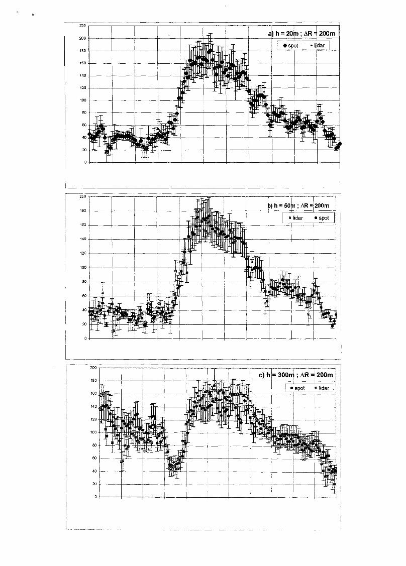
installed by AIRPARIF. Figure 4(a)-(c) shows the intercomparison between Lidar and spot

analyzers at the 3 different altitudes (ground level, 50 m, and 300 m) with a range resolution

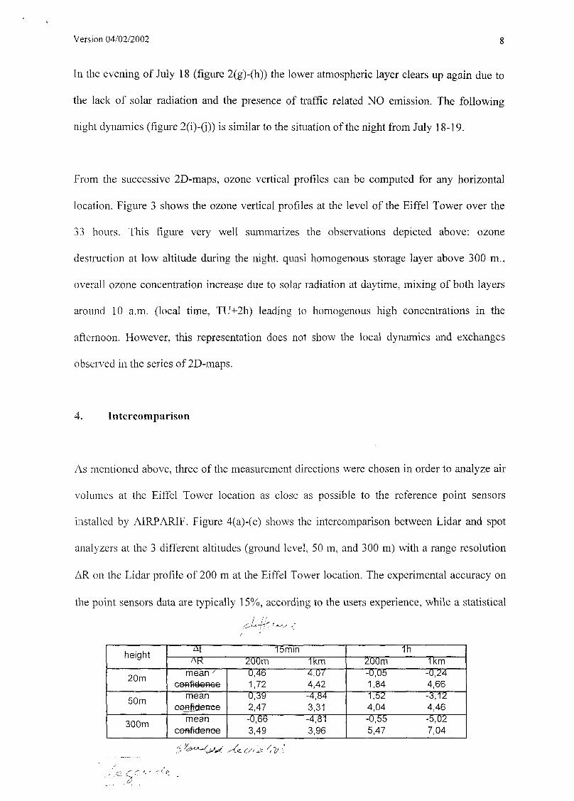
AR on the Lidar profile of 200 m at the Eiffel Tower location. The experimental accuracy on

the point sensors data are typically 15%, according to the users experience, while a statistical

height

20m

50m

300m

AtAR

mean /

meanoogftctertee

meancoftfiéenee

200m0,461,720,392,47-0,663,49

15min1km4,074,42-4,843,31-4,813,96

1h200m-0,051,841,524,04-0,555,47

1km-0,244,66-3,124,46-5,027,04

Ci/. '•

Version 04/02/2002 9

treatment of the Lidar data yields experimental standard deviation between 15 to 20 ug/m3

depending on the measurement configuration (temporal and spatial integration). As it can be

seen from these temporal profiles, the overall behavior as well as the absolute values are

excellent agreement at every altitudes and over the whole period. More precisely, figure 5

presents the histogram of differences between the ozone concentrations measured by the

sensors and the ones measured by Lidar: AC = Csensor - Cudar- The mean value of AC (offset)

is of the order of 1 ug/m3 , while the standard deviation on the difference (statistical errors)

o( AC) is only a few ug/m3 as well. This is particularly satisfactory since the measured values

spans a very broad concentration range from 20 to 180 ug/m3. It is also interesting to observe

that in stable and reasonably clear weather conditions, first order constant Rayleigh-Mie

corrections are sufficient to obtain very satisfactory results. In atmospheric conditions

exhibiting strong aerosol gradients this would obviously not be the case anymore.

Further intercomparison statistics have been performed for different Lidar spatial resolutions

(AR=200 m. and AR=1000 m ) and different "integration times" (15 minutes and 1 hour). On

this latter point, it is important to notice that in a 15 minutes measurement cycle, the actual

Lidar acquisition time for one reference point is only 1 minute (1000 shots averaged on each

direction of the scan, see section 3). For the hourly values, four successive Lidar

measurements at 15 minutes interval are averaged. The results are summarized in table 1. Best

agreement is found for AR=200 m. Averaging over 4 measurements (hourly comparison) does

not improve the statistical result, indicating that significant ozone concentration fluctuations

occur on shorter timescales. An interesting feature is that spatial averaging on longer

distances along the beam degrades the results as well. The reason is spatial fluctuations of the

ozone concentration. Averages over longer distances are less comparable to the air volume

measured by the spot monitor. This is very well illustrated by the observed negative offset

Version 04/02/2002 10

increasing with altitude on the 1 km averaged results (table 1). As shown in figure 2, ozone is

destroyed at low altitude at night. Since the beams are sent at finite angles (figure 1),

averaging over 1 km necessarily integrates lower ozone concentration values from low

altitude leading to a negative offset compared to the concentration at the Eiffel Tower level.

Spatial fluctuations of typical characteristic lengths of 50 m are also clearly observed on the

video clip or the snapshots of figure 2.

5. Conclusion

Very satisfactory Lidar-sensor intercomparison can be achieved in actual urban measurement

conditions results if the atmospheric spatial and temporal fluctuations are matched with the

respective resolutions of the devices. In particular, a compromise has to be found between two

opposite requirements: (1) spatial averaging improves the signal to noise ratio (SNR) of the

Lidar data and thus the accuracy of the concentration measurements, and (2) averaging over

longer paths provides mean values that are less comparable to spot measurements because of

local concentration gradients. In our conditions, the optimum parameters were AR=200 m

associated with an accuracy of 15 ug/mJ. However, these values are connected with the 1

minute time averaging. If only one measurement direction had been chosen, and

intercomparison with only one spot monitor, the Lidar data could have been continuously

averaged over 15 minutes, significantly improving the SNR. The accuracy and/or spatial

resolution could thus have been further improved accordingly. This strategy, however, would

have prevented 2D-mapping of the ozone concentration, which was the other main goal of the

campaign.

Acknowledgements

The authors acknowledge Jerome Kasparian for fruitful discussions and suggestions. J.P.W.

acknowledges the Institut Universitaire de France for support.

6. References

Version 04/02/2002 11

1. Beniston, M. , M. Beniston-Rebetez, H.J. Kôlsch, P. Rairoux, J.P. Wolf and L. Woste,

J.Geophys.Res., 95 (D7), 9879-9894 (1990)

2. Elight Laser Systems GmbH, Elight Laser Systems, Warthestrasse 21, D-14513 Teltow/Berlin;

http://www.elight.de (1999)

3. Godet Y., A. Thomasson, M. Nominé and T. Ménard, rapport INERIS (Institut National de

l'Environnement Industriel et des Risques) - Loi sur l'Ai r - Convention 13/98, Verneuil-en-

Hallate(1999)

4. Goers U.B., Optical Engineering 34(11), 3097-3102(1995)

5. GKSS Report 2000/24, ISSN 0344-9629, GKSS-Library, Postfach 1160, D-21494

Geesthacht (Germany) (2001)

6. Fiorani L., B. Calpini, A. Clappier, L. Jaquet, F. Mûller, H. van den Bergh, E. Durieux, A.

Ansmann, R. Neuber, P. Rairoux, U. Wandinger, Eds., Springer Verlag, Heidelberg, p. 367-

369(1996)

7. Frejafon. E., J. Kasparian, P. Rambaldi, B. Vezin, V. Boutou, J. Yu, M. Ulbricht, D.

Weidauer, B. Kraemer, T. Leisner, P. Rairoux, L. Woeste and J.P. Wolf, Europ. Phys. Journal

D 4, 231-238(1998)

8. De Saeger E, Report ERLAP 9, JRC, Ispra (1996)

9. Leighton P.A., Academic Press, New York (1961)

10. Measures R.M., Wiley, New York , (1984)

11. National Research Council, ISBN 0-309-04631-9, National Academy Press, Washington,

475 pp (1992)

12. VDI-DI N 4210, VDI-DI N Handbuch Reinhaltung der Luft, Band 5, Beuth Verlag Berlin

(1997)

13. Weidauer, D. ,P. Rairoux, M. Ulbricht, J.P. Wolf, L. Wôste, Advances in Atmospheric

Remote Sensing with Lidar, A. Ansmann, R. Neuber, P. Rairoux, 14. U. Wandinger, Eds.,

Springer Verlag, Heidelberg, pp. 423-426, (1996)

Version 04/02/2002 12

15. Weidauer D., H.D. Kambezidis, P. Rairoux, D. Mêlas, M. Ulbricht, Atmosph. Environ.

32,2173-2183(1998)

16. Wolf, J. P., in: Meyers, R. A. (Ed.), Encyclopedia of Analytical Chemistry, 3. J. Wiley &

Sons, New York, pp 2226-2247 (2000)

17. T. Ménard, E. Vindimian, Y. Godet, D. Weidauer, M. Ulbricht, P.Rambaldi, M. Douard,

J.P.Wolf, Poll.Atmos. 10-12, 105-119(1998)

18. Eickel, K.H. ,P. Rairoux, M. Ulbricht, D. Weidauer, K. Weber, J.P. Wolf, in Quality

Assurance and Standardisation of Remote Sensing Methods, K. Weber, ed. SPIE Vol. 3106

(1997)

Figure Captions

Fig I : Measurement site and principal Lidar measurement directions. The 3 lowest anglesare selected in order to match the location of reference ozone sensors on the Eiffel Tower.

Fig 2 : Continuous Lidar 2D-mapping of the ozone episode (snapshots form the video clip,which can be integrally seen on the electronic version of the paper).

Fig 3 : Evolution of the ozone vertical profiles, measured by Lidar, at the Eiffel Tower,location

Fig 4 : Intercomparison between reference spot analyzers and Lidar data at 3 differentaltitudes for 200 m of integration path at 15 min time interval (a,c).

Fig 5 : Histogram of the concentration differences AC between spot analyzers and Lidar.

-1600 -1400 -1200 -1000 -800 -600D i s t a n ce /m./

-400 -200

a) 17/07/1999-21h00 b) 18/07/1999-00h30

1400 -1200 -1000 -800 -EDO -400 -20 D 0

e) 18/07/1999 - 12h30

g) 18/07/1999-20h 15

1400 -1 200 -1000 -800 -600 -400 -200 0

-1400 -1200 -1000 -900 -600 -400 -200 0

j ) 19/07/1999 -08h00

-1800 -1600

j-250

| - 2 0 0

-150

-100

- 50

' Hg/m

ALTITUD E(mètres)

1400,

130a

1200

1100

1000

900

800

70O

600

500

400

300

200

100

OOhOO 02h00 04h00 06h00 08h00 lOhOO 12hOO 14h00 16h00 18hOO 20h00 22hOO OOhOO 02h00 O4hOO 06h00 O8hOO

18/07 18/07 18/07 18/07 18/07 18/07 18/07 18/07 18/07 18/07 18/07 18/07 19/07 19/07 19/07 19/07 19/07

h»300 m ;