LIBSVM: A Library for Support Vector Machines

Chih-Chung Chang and Chih-Jen LinDepartment of Computer Science

National Taiwan University, Taipei, TaiwanEmail: cjlin@csie.ntu.edu.tw

Initial version: 2001 Last updated: March 4, 2013

Abstract

LIBSVM is a library for Support Vector Machines (SVMs). We have beenactively developing this package since the year 2000. The goal is to help usersto easily apply SVM to their applications. LIBSVM has gained wide popu-larity in machine learning and many other areas. In this article, we presentall implementation details of LIBSVM. Issues such as solving SVM optimiza-tion problems, theoretical convergence, multi-class classification, probabilityestimates, and parameter selection are discussed in detail.

Keywords: Classification, LIBSVM, optimization, regression, support vector ma-chines, SVM

1 Introduction

Support Vector Machines (SVMs) are a popular machine learning method for classifi-

cation, regression, and other learning tasks. Since the year 2000, we have been devel-

oping the package LIBSVM as a library for support vector machines. The Web address

of the package is at http://www.csie.ntu.edu.tw/~cjlin/libsvm. LIBSVM is cur-

rently one of the most widely used SVM software. In this article,1 we present all

implementation details of LIBSVM. However, this article does not intend to teach

the practical use of LIBSVM. For instructions of using LIBSVM, see the README file

included in the package, the LIBSVM FAQ,2 and the practical guide by Hsu et al.

(2003). An earlier version of this article was published in Chang and Lin (2011).

LIBSVM supports the following learning tasks.

1This LIBSVM implementation document was created in 2001 and has been maintained at http://www.csie.ntu.edu.tw/~cjlin/papers/libsvm.pdf.

2LIBSVM FAQ: http://www.csie.ntu.edu.tw/~cjlin/libsvm/faq.html.

1

Table 1: Representative works in some domains that have successfully used LIBSVM.

Domain Representative worksComputer vision LIBPMK (Grauman and Darrell, 2005)Natural language processing Maltparser (Nivre et al., 2007)Neuroimaging PyMVPA (Hanke et al., 2009)Bioinformatics BDVal (Dorff et al., 2010)

1. SVC: support vector classification (two-class and multi-class).

2. SVR: support vector regression.

3. One-class SVM.

A typical use of LIBSVM involves two steps: first, training a data set to obtain a

model and second, using the model to predict information of a testing data set. For

SVC and SVR, LIBSVM can also output probability estimates. Many extensions of

LIBSVM are available at libsvmtools.3

The LIBSVM package is structured as follows.

1. Main directory: core C/C++ programs and sample data. In particular, the file

svm.cpp implements training and testing algorithms, where details are described

in this article.

2. The tool sub-directory: this sub-directory includes tools for checking data

format and for selecting SVM parameters.

3. Other sub-directories contain pre-built binary files and interfaces to other lan-

guages/software.

LIBSVM has been widely used in many areas. From 2000 to 2010, there were

more than 250,000 downloads of the package. In this period, we answered more than

10,000 emails from users. Table 1 lists representative works in some domains that

have successfully used LIBSVM.

This article is organized as follows. In Section 2, we describe SVM formulations

supported in LIBSVM: C-support vector classification (C-SVC), ν-support vector

classification (ν-SVC), distribution estimation (one-class SVM), ε-support vector re-

gression (ε-SVR), and ν-support vector regression (ν-SVR). Section 3 then discusses

performance measures, basic usage, and code organization. All SVM formulations

3 LIBSVM Tools: http://www.csie.ntu.edu.tw/~cjlin/libsvmtools.

2

supported in LIBSVM are quadratic minimization problems. We discuss the opti-

mization algorithm in Section 4. Section 5 describes two implementation techniques

to reduce the running time for minimizing SVM quadratic problems: shrinking and

caching. LIBSVM provides some special settings for unbalanced data; details are

in Section 6. Section 7 discusses our implementation for multi-class classification.

Section 8 presents how to transform SVM decision values into probability values. Pa-

rameter selection is important for obtaining good SVM models. Section 9 presents a

simple and useful parameter selection tool in LIBSVM. Finally, Section 10 concludes

this work.

2 SVM Formulations

LIBSVM supports various SVM formulations for classification, regression, and distri-

bution estimation. In this section, we present these formulations and give correspond-

ing references. We also show performance measures used in LIBSVM.

2.1 C-Support Vector Classification

Given training vectors xi ∈ Rn, i = 1, . . . , l, in two classes, and an indicator vector

y ∈ Rl such that yi ∈ {1,−1}, C-SVC (Boser et al., 1992; Cortes and Vapnik, 1995)

solves the following primal optimization problem.

minw,b,ξ

1

2wTw + C

l∑i=1

ξi (1)

subject to yi(wTφ(xi) + b) ≥ 1− ξi,

ξi ≥ 0, i = 1, . . . , l,

where φ(xi) maps xi into a higher-dimensional space and C > 0 is the regularization

parameter. Due to the possible high dimensionality of the vector variable w, usually

we solve the following dual problem.

minα

1

2αTQα− eTα

subject to yTα = 0, (2)

0 ≤ αi ≤ C, i = 1, . . . , l,

where e = [1, . . . , 1]T is the vector of all ones, Q is an l by l positive semidefinite

matrix, Qij ≡ yiyjK(xi,xj), and K(xi,xj) ≡ φ(xi)Tφ(xj) is the kernel function.

3

After problem (2) is solved, using the primal-dual relationship, the optimal w

satisfies

w =l∑

i=1

yiαiφ(xi) (3)

and the decision function is

sgn(wTφ(x) + b

)= sgn

(l∑

i=1

yiαiK(xi,x) + b

).

We store yiαi ∀i, b, label names,4 support vectors, and other information such as

kernel parameters in the model for prediction.

2.2 ν-Support Vector Classification

The ν-support vector classification (Scholkopf et al., 2000) introduces a new parameter

ν ∈ (0, 1]. It is proved that ν an upper bound on the fraction of training errors and

a lower bound of the fraction of support vectors.

Given training vectors xi ∈ Rn, i = 1, . . . , l, in two classes, and a vector y ∈ Rl

such that yi ∈ {1,−1}, the primal optimization problem is

minw,b,ξ,ρ

1

2wTw − νρ+

1

l

l∑i=1

ξi

subject to yi(wTφ(xi) + b) ≥ ρ− ξi, (4)

ξi ≥ 0, i = 1, . . . , l, ρ ≥ 0.

The dual problem is

minα

1

2αTQα

subject to 0 ≤ αi ≤ 1/l, i = 1, . . . , l, (5)

eTα ≥ ν, yTα = 0,

where Qij = yiyjK(xi,xj). Chang and Lin (2001) show that problem (5) is feasible

if and only if

ν ≤ 2 min(#yi = +1,#yi = −1)

l≤ 1,

so the usable range of ν is smaller than (0, 1].

4In LIBSVM, any integer can be a label name, so we map label names to ±1 by assigning the firsttraining instance to have y1 = +1.

4

The decision function is

sgn

(l∑

i=1

yiαiK(xi,x) + b

).

It is shown that eTα ≥ ν can be replaced by eTα = ν (Crisp and Burges, 2000;

Chang and Lin, 2001). In LIBSVM, we solve a scaled version of problem (5) because

numerically αi may be too small due to the constraint αi ≤ 1/l.

minα

1

2αTQα

subject to 0 ≤ αi ≤ 1, i = 1, . . . , l, (6)

eT α = νl, yT α = 0.

If α is optimal for the dual problem (5) and ρ is optimal for the primal problem

(4), Chang and Lin (2001) show that α/ρ is an optimal solution of C-SVM with

C = 1/(ρl). Thus, in LIBSVM, we output (α/ρ, b/ρ) in the model.5

2.3 Distribution Estimation (One-class SVM)

One-class SVM was proposed by Scholkopf et al. (2001) for estimating the support of

a high-dimensional distribution. Given training vectors xi ∈ Rn, i = 1, . . . , l without

any class information, the primal problem of one-class SVM is

minw,ξ,ρ

1

2wTw − ρ+

1

νl

l∑i=1

ξi

subject to wTφ(xi) ≥ ρ− ξi,

ξi ≥ 0, i = 1, . . . , l.

The dual problem is

minα

1

2αTQα

subject to 0 ≤ αi ≤ 1/(νl), i = 1, . . . , l, (7)

eTα = 1,

where Qij = K(xi,xj) = φ(xi)Tφ(xj). The decision function is

sgn

(l∑

i=1

αiK(xi,x)− ρ

).

5More precisely, solving (6) obtains ρ = ρl. Because α = lα, we have α/ρ = α/ρ. Hence, inLIBSVM, we calculate α/ρ.

5

Similar to the case of ν-SVC, in LIBSVM, we solve a scaled version of (7).

minα

1

2αTQα

subject to 0 ≤ αi ≤ 1, i = 1, . . . , l, (8)

eTα = νl.

2.4 ε-Support Vector Regression (ε-SVR)

Consider a set of training points, {(x1, z1), . . . , (xl, zl)}, where xi ∈ Rn is a feature

vector and zi ∈ R1 is the target output. Under given parameters C > 0 and ε > 0,

the standard form of support vector regression (Vapnik, 1998) is

minw,b,ξ,ξ∗

1

2wTw + C

l∑i=1

ξi + Cl∑

i=1

ξ∗i

subject to wTφ(xi) + b− zi ≤ ε+ ξi,

zi −wTφ(xi)− b ≤ ε+ ξ∗i ,

ξi, ξ∗i ≥ 0, i = 1, . . . , l.

The dual problem is

minα,α∗

1

2(α−α∗)TQ(α−α∗) + ε

l∑i=1

(αi + α∗i ) +l∑

i=1

zi(αi − α∗i )

subject to eT (α−α∗) = 0, (9)

0 ≤ αi, α∗i ≤ C, i = 1, . . . , l,

where Qij = K(xi,xj) ≡ φ(xi)Tφ(xj).

After solving problem (9), the approximate function is

l∑i=1

(−αi + α∗i )K(xi,x) + b.

In LIBSVM, we output α∗ −α in the model.

2.5 ν-Support Vector Regression (ν-SVR)

Similar to ν-SVC, for regression, Scholkopf et al. (2000) use a parameter ν ∈ (0, 1]

to control the number of support vectors. The parameter ε in ε-SVR becomes a

6

parameter here. With (C, ν) as parameters, ν-SVR solves

minw,b,ξ,ξ∗,ε

1

2wTw + C(νε+

1

l

l∑i=1

(ξi + ξ∗i ))

subject to (wTφ(xi) + b)− zi ≤ ε+ ξi,

zi − (wTφ(xi) + b) ≤ ε+ ξ∗i ,

ξi, ξ∗i ≥ 0, i = 1, . . . , l, ε ≥ 0.

The dual problem is

minα,α∗

1

2(α−α∗)TQ(α−α∗) + zT (α−α∗)

subject to eT (α−α∗) = 0, eT (α+α∗) ≤ Cν, (10)

0 ≤ αi, α∗i ≤ C/l, i = 1, . . . , l.

The approximate function is

l∑i=1

(−αi + α∗i )K(xi,x) + b.

Similar to ν-SVC, Chang and Lin (2002) show that the inequality eT (α+α∗) ≤ Cν

can be replaced by an equality. Moreover, C/l may be too small because users often

choose C to be a small constant like one. Thus, in LIBSVM, we treat the user-

specified regularization parameter as C/l. That is, C = C/l is what users specified

and LIBSVM solves the following problem.

minα,α∗

1

2(α−α∗)TQ(α−α∗) + zT (α−α∗)

subject to eT (α−α∗) = 0, eT (α+α∗) = Clν,

0 ≤ αi, α∗i ≤ C, i = 1, . . . , l.

Chang and Lin (2002) prove that ε-SVR with parameters (C, ε) has the same solution

as ν-SVR with parameters (lC, ν).

3 Performance Measures, Basic Usage, and Code

Organization

This section describes LIBSVM’s evaluation measures, shows some simple examples

of running LIBSVM, and presents the code structure.

7

3.1 Performance Measures

After solving optimization problems listed in previous sections, users can apply de-

cision functions to predict labels (target values) of testing data. Let x1, . . . ,xl be

the testing data and f(x1), . . . , f(xl) be decision values (target values for regression)

predicted by LIBSVM. If the true labels (true target values) of testing data are known

and denoted as yi, . . . , yl, we evaluate the prediction results by the following measures.

3.1.1 Classification

Accuracy

=# correctly predicted data

# total testing data× 100%

3.1.2 Regression

LIBSVM outputs MSE (mean squared error) and r2 (squared correlation coefficient).

MSE =1

l

l∑i=1

(f(xi)− yi)2 ,

r2 =

(l∑l

i=1 f(xi)yi −∑l

i=1 f(xi)∑l

i=1 yi

)2(l∑l

i=1 f(xi)2 −(∑l

i=1 f(xi))2)(

l∑l

i=1 y2i −

(∑li=1 yi

)2) .

3.2 A Simple Example of Running LIBSVM

While detailed instructions of using LIBSVM are available in the README file of the

package and the practical guide by Hsu et al. (2003), here we give a simple example.

LIBSVM includes a sample data set heart scale of 270 instances. We split the

data to a training set heart scale.tr (170 instances) and a testing set heart scale.te.

$ python tools/subset.py heart_scale 170 heart_scale.tr heart_scale.te

The command svm-train solves an SVM optimization problem to produce a model.6

$ ./svm-train heart_scale.tr

*

optimization finished, #iter = 87

nu = 0.471645

6The default solver is C-SVC using the RBF kernel (48) with C = 1 and γ = 1/n.

8

obj = -67.299458, rho = 0.203495

nSV = 88, nBSV = 72

Total nSV = 88

Next, the command svm-predict uses the obtained model to classify the testing set.

$ ./svm-predict heart_scale.te heart_scale.tr.model output

Accuracy = 83% (83/100) (classification)

The file output contains predicted class labels.

3.3 Code Organization

All LIBSVM’s training and testing algorithms are implemented in the file svm.cpp.

The two main sub-routines are svm train and svm predict. The training procedure

is more sophisticated, so we give the code organization in Figure 1.

From Figure 1, for classification, svm train decouples a multi-class problem to

two-class problems (see Section 7) and calls svm train one several times. For re-

gression and one-class SVM, it directly calls svm train one. The probability outputs

for classification and regression are also handled in svm train. Then, according

to the SVM formulation, svm train one calls a corresponding sub-routine such as

solve c svc for C-SVC and solve nu svc for ν-SVC. All solve * sub-routines call

the solver Solve after preparing suitable input values. The sub-routine Solve min-

imizes a general form of SVM optimization problems; see (11) and (22). Details of

the sub-routine Solve are described in Sections 4-6.

4 Solving the Quadratic Problems

This section discusses algorithms used in LIBSVM to solve dual quadratic problems

listed in Section 2. We split the discussion to two parts. The first part considers

optimization problems with one linear constraint, while the second part checks those

with two linear constraints.

9

svm train

svm train one

solve c svc solve nu svc

Solve

. . . Various SVM formulations

Two-class SVC, SVR, one-class SVM

Main training sub-routine

Solving problems (11) and (22)

Figure 1: LIBSVM’s code organization for training. All sub-routines are in svm.cpp.

4.1 Quadratic Problems with One Linear Constraint: C-SVC,ε-SVR, and One-class SVM

We consider the following general form of C-SVC, ε-SVR, and one-class SVM.

minα

f(α)

subject to yTα = ∆, (11)

0 ≤ αt ≤ C, t = 1, . . . , l,

where

f(α) ≡ 1

2αTQα+ pTα

and yt = ±1, t = 1, . . . , l. The constraint yTα = 0 is called a linear constraint. It can

be clearly seen that C-SVC and one-class SVM are already in the form of problem

(11). For ε-SVR, we use the following reformulation of Eq. (9).

minα,α∗

1

2

[(α∗)T ,αT

] [ Q −Q−Q Q

] [α∗

α

]+[εeT − zT , εeT + zT

] [α∗α

]subject to yT

[α∗

α

]= 0, 0 ≤ αt, α

∗t ≤ C, t = 1, . . . , l,

where

y = [1, . . . , 1︸ ︷︷ ︸l

,−1, . . . ,−1︸ ︷︷ ︸l

]T .

We do not assume that Q is positive semi-definite (PSD) because sometimes non-PSD

kernel matrices are used.

10

4.1.1 Decomposition Method for Dual Problems

The main difficulty for solving problem (11) is that Q is a dense matrix and may be

too large to be stored. In LIBSVM, we consider a decomposition method to conquer

this difficulty. Some earlier works on decomposition methods for SVM include, for

example, Osuna et al. (1997a); Joachims (1998); Platt (1998); Keerthi et al. (2001);

Hsu and Lin (2002b). Subsequent developments include, for example, Fan et al.

(2005); Palagi and Sciandrone (2005); Glasmachers and Igel (2006). A decomposition

method modifies only a subset of α per iteration, so only some columns of Q are

needed. This subset of variables, denoted as the working set B, leads to a smaller

optimization sub-problem. An extreme case of the decomposition methods is the

Sequential Minimal Optimization (SMO) (Platt, 1998), which restricts B to have only

two elements. Then, at each iteration, we solve a simple two-variable problem without

needing any optimization software. LIBSVM considers an SMO-type decomposition

method proposed in Fan et al. (2005).

Algorithm 1 (An SMO-type decomposition method in Fan et al., 2005)

1. Find α1 as the initial feasible solution. Set k = 1.

2. If αk is a stationary point of problem (2), stop. Otherwise, find a two-element

working set B = {i, j} by WSS 1 (described in Section 4.1.2). Define N ≡{1, . . . , l}\B. Let αkB and αkN be sub-vectors of αk corresponding to B and N ,

respectively.

3. If aij ≡ Kii +Kjj − 2Kij > 0,7

Solve the following sub-problem with the variable αB = [αi αj]T .

minαi,αj

1

2

[αi αj

] [Qii Qij

Qij Qjj

] [αiαj

]+ (pB +QBNα

kN)T

[αiαj

]subject to 0 ≤ αi, αj ≤ C, (12)

yiαi + yjαj = ∆− yTNαkN ,

else

7We abbreviate K(xi,xj) to Kij .

11

Let τ be a small positive constant and solve

minαi,αj

1

2

[αi αj

] [Qii Qij

Qij Qjj

] [αiαj

]+ (pB +QBNα

kN)T

[αiαj

]+τ − aij

4((αi − αki )2 + (αj − αkj )2) (13)

subject to constraints of problem (12).

4. Setαk+1B to be the optimal solution of sub-problem (12) or (13), andαk+1

N ≡ αkN .

Set k ← k + 1 and go to Step 2.

Note that B is updated at each iteration, but for simplicity, we use B instead of

Bk. If Q is PSD, then aij > 0. Thus sub-problem (13) is used only to handle the

situation where Q is non-PSD.

4.1.2 Stopping Criteria and Working Set Selection

The Karush-Kuhn-Tucker (KKT) optimality condition of problem (11) implies that

a feasible α is a stationary point of (11) if and only if there exists a number b and

two nonnegative vectors λ and ξ such that

∇f(α) + by = λ− ξ,

λiαi = 0, ξi(C − αi) = 0, λi ≥ 0, ξi ≥ 0, i = 1, . . . , l, (14)

where ∇f(α) ≡ Qα + p is the gradient of f(α). Note that if Q is PSD, from the

primal-dual relationship, ξ, b, and w generated by Eq. (3) form an optimal solution

of the primal problem. The condition (14) can be rewritten as

∇if(α) + byi

{≥ 0 if αi < C,

≤ 0 if αi > 0.(15)

Since yi = ±1, condition (15) is equivalent to that there exists b such that

m(α) ≤ b ≤M(α),

where

m(α) ≡ maxi∈Iup(α)

−yi∇if(α) and M(α) ≡ mini∈Ilow(α)

−yi∇if(α),

and

Iup(α) ≡ {t | αt < C, yt = 1 or αt > 0, yt = −1}, and

Ilow(α) ≡ {t | αt < C, yt = −1 or αt > 0, yt = 1}.

12

That is, a feasible α is a stationary point of problem (11) if and only if

m(α) ≤M(α). (16)

From (16), a suitable stopping condition is

m(αk)−M(αk) ≤ ε, (17)

where ε is the tolerance.

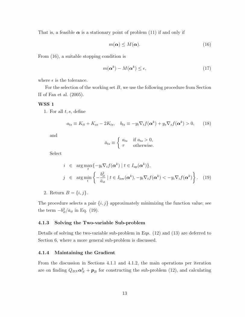
For the selection of the working set B, we use the following procedure from Section

II of Fan et al. (2005).

WSS 1

1. For all t, s, define

ats ≡ Ktt +Kss − 2Kts, bts ≡ −yt∇tf(αk) + ys∇sf(αk) > 0, (18)

and

ats ≡{ats if ats > 0,τ otherwise.

Select

i ∈ arg maxt{−yt∇tf(αk) | t ∈ Iup(αk)},

j ∈ arg mint

{− b

2it

ait| t ∈ Ilow(αk),−yt∇tf(αk) < −yi∇if(αk)

}. (19)

2. Return B = {i, j}.

The procedure selects a pair {i, j} approximately minimizing the function value; see

the term −b2it/ait in Eq. (19).

4.1.3 Solving the Two-variable Sub-problem

Details of solving the two-variable sub-problem in Eqs. (12) and (13) are deferred to

Section 6, where a more general sub-problem is discussed.

4.1.4 Maintaining the Gradient

From the discussion in Sections 4.1.1 and 4.1.2, the main operations per iteration

are on finding QBNαkN + pB for constructing the sub-problem (12), and calculating

13

∇f(αk) for the working set selection and the stopping condition. These two opera-

tions can be considered together because

QBNαkN + pB = ∇Bf(αk)−QBBα

kB (20)

and

∇f(αk+1) = ∇f(αk) +Q:,B(αk+1B −αkB), (21)

where |B| � |N | and Q:,B is the sub-matrix of Q including columns in B. If at the

kth iteration we already have ∇f(αk), then Eq. (20) can be used to construct the

sub-problem. After the sub-problem is solved, Eq. (21) is employed to have the next

∇f(αk+1). Therefore, LIBSVM maintains the gradient throughout the decomposition

method.

4.1.5 The Calculation of b or ρ

After the solution α of the dual optimization problem is obtained, the variables b or

ρ must be calculated as they are used in the decision function.

Note that b of C-SVC and ε-SVR plays the same role as −ρ in one-class SVM, so

we define ρ = −b and discuss how to find ρ. If there exists αi such that 0 < αi < C,

then from the KKT condition (16), ρ = yi∇if(α). In LIBSVM, for numerical stability,

we average all these values.

ρ =

∑i:0<αi<C

yi∇if(α)

|{i | 0 < αi < C}|.

For the situation that no αi satisfying 0 < αi < C, the KKT condition (16) becomes

−M(α) = max{yi∇if(α) | αi = 0, yi = −1 or αi = C, yi = 1}

≤ ρ

≤ −m(α) = min{yi∇if(α) | αi = 0, yi = 1 or αi = C, yi = −1}.

We take ρ the midpoint of the preceding range.

4.1.6 Initial Values

Algorithm 1 requires an initial feasible α. For C-SVC and ε-SVR, because the zero

vector is feasible, we select it as the initial α.

For one-class SVM, the scaled form (8) requires that

0 ≤ αi ≤ 1, andl∑

i=1

αi = νl.

14

We let the first bνlc elements have αi = 1 and the (bνlc + 1)st element have αi =

νl − bνlc.

4.1.7 Convergence of the Decomposition Method

Fan et al. (2005, Section III) and Chen et al. (2006) discuss the convergence of Algo-

rithm 1 in detail. For the rate of linear convergence, List and Simon (2009) prove a

result without making the assumption used in Chen et al. (2006).

4.2 Quadratic Problems with Two Linear Constraints: ν-SVC and ν-SVR

From problems (6) and (10), both ν-SVC and ν-SVR can be written as the following

general form.

minα

1

2αTQα+ pTα

subject to yTα = ∆1, (22)

eTα = ∆2,

0 ≤ αt ≤ C, t = 1, . . . , l.

The main difference between problems (11) and (22) is that (22) has two linear

constraints yTα = ∆1 and eTα = ∆2. The optimization algorithm is very similar to

that for (11), so we describe only differences.

4.2.1 Stopping Criteria and Working Set Selection

Let f(α) be the objective function of problem (22). By the same derivation in Sec-

tion 4.1.2, The KKT condition of problem (22) implies that there exist b and ρ such

that

∇if(α)− ρ+ byi

{≥ 0 if αi < C,

≤ 0 if αi > 0.(23)

Define

r1 ≡ ρ− b and r2 ≡ ρ+ b. (24)

If yi = 1, (23) becomes

∇if(α)− r1

{≥ 0 if αi < C,

≤ 0 if αi > 0.(25)

15

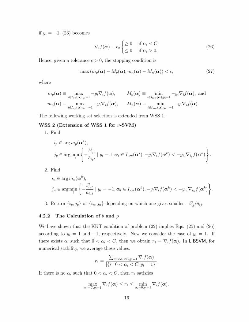
if yi = −1, (23) becomes

∇if(α)− r2

{≥ 0 if αi < C,

≤ 0 if αi > 0.(26)

Hence, given a tolerance ε > 0, the stopping condition is

max (mp(α)−Mp(α),mn(α)−Mn(α)) < ε, (27)

where

mp(α) ≡ maxi∈Iup(α),yi=1

−yi∇if(α), Mp(α) ≡ mini∈Ilow(α),yi=1

−yi∇if(α), and

mn(α) ≡ maxi∈Iup(α),yi=−1

−yi∇if(α), Mn(α) ≡ mini∈Ilow(α),yi=−1

−yi∇if(α).

The following working set selection is extended from WSS 1.

WSS 2 (Extension of WSS 1 for ν-SVM)

1. Find

ip ∈ argmp(αk),

jp ∈ arg mint

{−b2ipt

aipt| yt = 1,αt ∈ Ilow(αk),−yt∇tf(αk) < −yip∇ipf(αk)

}.

2. Find

in ∈ argmn(αk),

jn ∈ arg mint

{−b2int

aint| yt = −1,αt ∈ Ilow(αk),−yt∇tf(αk) < −yin∇inf(αk)

}.

3. Return {ip, jp} or {in, jn} depending on which one gives smaller −b2ij/aij.

4.2.2 The Calculation of b and ρ

We have shown that the KKT condition of problem (22) implies Eqs. (25) and (26)

according to yi = 1 and −1, respectively. Now we consider the case of yi = 1. If

there exists αi such that 0 < αi < C, then we obtain r1 = ∇if(α). In LIBSVM, for

numerical stability, we average these values.

r1 =

∑i:0<αi<C,yi=1∇if(α)

|{i | 0 < αi < C, yi = 1}|.

If there is no αi such that 0 < αi < C, then r1 satisfies

maxαi=C,yi=1

∇if(α) ≤ r1 ≤ minαi=0,yi=1

∇if(α).

16

We take r1 the midpoint of the previous range.

For the case of yi = −1, we can calculate r2 in a similar way.

After r1 and r2 are obtained, from Eq. (24),

ρ =r1 + r2

2and − b =

r1 − r2

2.

4.2.3 Initial Values

For ν-SVC, the scaled form (6) requires that

0 ≤ αi ≤ 1,∑i:yi=1

αi =νl

2, and

∑i:yi=−1

αi =νl

2.

We let the first νl/2 elements of αi with yi = 1 to have the value one.8 The situation

for yi = −1 is similar. The same setting is applied to ν-SVR.

5 Shrinking and Caching

This section discusses two implementation tricks (shrinking and caching) for the de-

composition method and investigates the computational complexity of Algorithm 1.

5.1 Shrinking

An optimal solution α of the SVM dual problem may contain some bounded elements

(i.e., αi = 0 or C). These elements may have already been bounded in the middle of

the decomposition iterations. To save the training time, the shrinking technique tries

to identify and remove some bounded elements, so a smaller optimization problem is

solved (Joachims, 1998). The following theorem theoretically supports the shrinking

technique by showing that at the final iterations of Algorithm 1 in Section 4.1.2, only

a small set of variables is still changed.

Theorem 5.1 (Theorem IV in Fan et al., 2005) Consider problem (11) and as-

sume Q is positive semi-definite.

1. The following set is independent of any optimal solution α.

I ≡ {i | −yi∇if(α) > M(α) or − yi∇if(α) < m(α)}.

Further, for every i ∈ I, problem (11) has a unique and bounded optimal solution

at αi.

8Special care must be made as νl/2 may not be an integer. See also Section 4.1.6.

17

2. Assume Algorithm 1 generates an infinite sequence {αk}. There exists k such

that after k ≥ k, every αki , i ∈ I has reached the unique and bounded optimal

solution. That is, αki remains the same in all subsequent iterations. In addition,

∀k ≥ k:

i 6∈ {t |M(αk) ≤ −yt∇tf(αk) ≤ m(αk)}.

If we denote A as the set containing elements not shrunk at the kth iteration,

then instead of solving problem (11), the decomposition method works on a smaller

problem.

minαA

1

2αTAQAAαA + (pA +QANα

kN)TαA

subject to 0 ≤ αi ≤ C, ∀i ∈ A, (28)

yTAαA = ∆− yTNαkN ,

where N = {1, . . . , l}\A is the set of shrunk variables. Note that in LIBSVM, we

always rearrange elements of α,y, and p to maintain that A = {1, . . . , |A|}. Details

of the index rearrangement are in Section 5.4.

After solving problem (28), we may find that some elements are wrongly shrunk.

When that happens, the original problem (11) is reoptimized from a starting point

α = [ αAαN ], where αA is optimal for problem (28) and αN corresponds to shrunk

bounded variables.

In LIBSVM, we start the shrinking procedure in an early stage. The procedure is

as follows.

1. After every min(l, 1000) iterations, we try to shrink some variables. Note that

throughout the iterative process, we have

m(αk) > M(αk) (29)

because the condition (17) is not satisfied yet. Following Theorem 5.1, we

conjecture that variables in the following set can be shrunk.

{t | −yt∇tf(αk) > m(αk), t ∈ Ilow(αk), αkt is bounded}∪

{t | −yt∇tf(αk) < M(αk), t ∈ Iup(αk), αkt is bounded}

= {t | −yt∇tf(αk) > m(αk), αkt = C, yt = 1 or αkt = 0, yt = −1}∪

{t | −yt∇tf(αk) < M(αk), αkt = 0, yt = 1 or αkt = C, yt = −1}.

(30)

Thus, the size of the set A is gradually reduced in every min(l, 1000) iterations.

The problem (28), and the way of calculating m(αk) and M(αk) are adjusted

accordingly.

18

2. The preceding shrinking strategy is sometimes too aggressive. Hence, when the

decomposition method achieves the following condition for the first time.

m(αk) ≤M(αk) + 10ε, (31)

where ε is the specified stopping tolerance, we reconstruct the gradient (details

in Section 5.3). Then, the shrinking procedure can be performed based on more

accurate information.

3. Once the stopping condition

m(αk) ≤M(αk) + ε (32)

of the smaller problem (28) is reached, we must check if the stopping condition

of the original problem (11) has been satisfied. If not, then we reactivate all

variables by setting A = {1, . . . , l} and start the same shrinking procedure on

the problem (28).

Note that in solving the shrunk problem (28), we only maintain its gradient

QAAαA + QANαN + pA (see also Section 4.1.4). Hence, when we reactivate

all variables to reoptimize the problem (11), we must reconstruct the whole

gradient ∇f(α). Details are discussed in Section 5.3.

For ν-SVC and ν-SVR, because the stopping condition (27) is different from (17),

variables being shrunk are different from those in (30). For yt = 1, we shrink elements

in the following set

{t | −yt∇tf(αk) > mp(αk), αt = C, yt = 1}∪

{t | −yt∇tf(αk) < Mp(αk), αt = 0, yt = 1}.

For yt = −1, we consider the following set.

{t | −yt∇tf(αk) > mn(αk), αt = 0, yt = −1}∪

{t | −yt∇tf(αk) < Mn(αk), αt = C, yt = −1}.

5.2 Caching

Caching is an effective technique for reducing the computational time of the decompo-

sition method. Because Q may be too large to be stored in the computer memory, Qij

elements are calculated as needed. We can use available memory (called kernel cache)

to store some recently used Qij (Joachims, 1998). Then, some kernel elements may

19

not need to be recalculated. Theorem 5.1 also supports the use of caching because

in final iterations, only certain columns of the matrix Q are still needed. If the cache

already contains these columns, we can save kernel evaluations in final iterations.

In LIBSVM, we consider a simple least-recent-use caching strategy. We use a

circular list of structures, where each structure is defined as follows.

struct head_t

{

head_t *prev, *next; // a circular list

Qfloat *data;

int len; // data[0,len) is cached in this entry

};

A structure stores the first len elements of a kernel column. Using pointers prev and

next, it is easy to insert or delete a column. The circular list is maintained so that

structures are ordered from the least-recent-used one to the most-recent-used one.

Because of shrinking, columns cached in the computer memory may be in different

length. Assume the ith column is needed and Q1:t,i have been cached. If t ≤ |A|, we

calculate Qt+1:|A|,i and store Q1:|A|,i in the cache. If t > |A|, the desired Q1:|A|,i are

already in the cache. In this situation, we do not change the cached contents of the

ith column.

5.3 Reconstructing the Gradient

If condition (31) or (32) is satisfied, LIBSVM reconstructs the gradient. Because

∇if(α), i = 1, . . . , |A| have been maintained in solving the smaller problem (28),

what we need is to calculate ∇if(α), i = |A| + 1, . . . , l. To decrease the cost of this

reconstruction, throughout iterations we maintain a vector G ∈ Rl.

Gi = C∑

j:αj=C

Qij, i = 1, . . . , l. (33)

Then, for i /∈ A,

∇if(α) =l∑

j=1

Qijαj + pi = Gi + pi +∑j:j∈A

0<αj<C

Qijαj. (34)

Note that we use the fact that if j /∈ A, then αj = 0 or C.

20

The calculation of ∇f(α) via Eq. (34) involves a two-level loop over i and j.

Using i or j first may result in a very different number of Qij evaluations. We discuss

the differences next.

1. i first: for |A| + 1 ≤ i ≤ l, calculate Qi,1:|A|. Although from Eq. (34), only

{Qij | 0 < αj < C, j ∈ A} are needed, our implementation obtains all Qi,1:|A|

(i.e., {Qij | j ∈ A}). Hence, this case needs at most

(l − |A|) · |A| (35)

kernel evaluations. Note that LIBSVM uses a column-based caching implemen-

tation. Due to the symmetry of Q, Qi,1:|A| is part of Q’s ith column and may

have been cached. Thus, Eq. (35) is only an upper bound.

2. j first: let

F ≡ {j | 1 ≤ j ≤ |A| and 0 < αj < C}.

For each j ∈ F , calculate Q1:l,j. Though only Q|A|+1:l,j is needed in calculating

∇if(α), i = |A|+ 1, . . . , l, we must get the whole column because of our cache

implementation.9 Thus, this strategy needs no more than

l · |F | (36)

kernel evaluations. This is an upper bound because certain kernel columns (e.g.,

Q1:|A|,j, j ∈ A) may be already in the cache and do not need to be recalculated.

We may choose a method by comparing (35) and (36). However, the decision depends

on whether Q’s elements have been cached. If the cache is large enough, then elements

of Q’s first |A| columns tend to be in the cache because they have been used recently.

In contrast, Qi,1:|A|, i /∈ A needed by method 1 may be less likely in the cache because

columns not in A are not used to solve problem (28). In such a situation, method 1

may require almost (l−|A|) · |A| kernel valuations, while method 2 needs much fewer

evaluations than l · |F |.Because method 2 takes an advantage of the cache implementation, we slightly

lower the estimate in Eq. (36) and use the following rule to decide the method of

calculating Eq. (34):If (l/2) · |F | > (l − |A|) · |A|

use method 1Else

use method 2

9We always store the first |A| elements of a column.

21

This rule may not give the optimal choice because we do not take the cache contents

into account. However, we argue that in the worst scenario, the selected method by

the preceding rule is only slightly slower than the other method. This result can be

proved by making the following assumptions.

• A LIBSVM training procedure involves only two gradient reconstructions. The

first is performed when the 10ε tolerance is achieved; see Eq. (31). The second

is in the end of the training procedure.

• Our rule assigns the same method to perform the two gradient reconstructions.

Moreover, these two reconstructions cost a similar amount of time.

We refer to “total training time of method x” as the whole LIBSVM training time

(where method x is used for reconstructing gradients), and “reconstruction time of

method x” as the time of one single gradient reconstruction via method x. We then

consider two situations.

1. Method 1 is chosen, but method 2 is better.

We have

Total time of method 1

≤ (Total time of method 2) + 2 · (Reconstruction time of method 1)

≤ 2 · (Total time of method 2). (37)

We explain the second inequality in detail. Method 2 for gradient reconstruction

requires l · |F | kernel elements; however, the number of kernel evaluations may

be smaller because some elements have been cached. Therefore,

l · |F | ≤ Total time of method 2. (38)

Because method 1 is chosen and Eq. (35) is an upper bound,

2 · (Reconstruction time of method 1) ≤ 2 · (l − |A|) · |A| < l · |F |. (39)

Combining inequalities (38) and (39) leads to (37).

2. Method 2 is chosen, but method 1 is better.

We consider the worst situation where Q’s first |A| columns are not in the cache.

As |A|+1, . . . , l are indices of shrunk variables, most likely the remaining l−|A|

22

Table 2: A comparison between two gradient reconstruction methods. The decom-position method reconstructs the gradient twice after satisfying conditions (31) and(32). We show in each row the number of kernel evaluations of a reconstruction. Wecheck two cache sizes to reflect the situations with/without enough cache. The lasttwo rows give the total training time (gradient reconstructions and other operations)in seconds. We use the RBF kernel K(xi,xj) = exp(−γ‖xi − xj‖2).

(a) a7a: C = 1, γ = 4, ε = 0.001.

l = 16, 100 Cache = 1,000 MB Cache = 10 MBReconstruction |F | |A| Method 1 Method 2 Method 1 Method 2First 10,597 12,476 0 21,470,526 45,213,024 170,574,272Second 10,630 12,476 0 0 45,213,024 171,118,048

Training time ⇒ 102s 108s 341s 422sNo shrinking: 111s No shrinking: 381s

(b) ijcnn1: C = 16, γ = 4, ε = 0.5.

l = 49, 900 Cache = 1,000 MB Cache = 10 MBReconstruction |F | |A| Method 1 Method 2 Method 1 Method 2First 1,767 43,678 274,297,840 5,403,072 275,695,536 88,332,330Second 2,308 6,023 263,843,538 28,274,195 264,813,241 115,346,805

Training time ⇒ 189s 46s 203s 116sNo shrinking: 42s No shrinking: 87s

columns of Q are not in the cache either and (l − |A|) · |A| kernel evaluations

are needed for method 1. Because l · |F | ≤ 2 · (l − |A|) · |A|,

(Reconstruction time of method 2) ≤ 2 · (Reconstruction time of method 1).

Therefore,

Total time of method 2

≤ (Total time of method 1) + 2 · (Reconstruction time of method 1)

≤ 2 · (Total time of method 1).

Table 2 compares the number of kernel evaluations in reconstructing the gradient.

We consider problems a7a and ijcnn1.10 Clearly, the proposed rule selects the better

method for both problems. We implement this technique after version 2.88 of LIBSVM.

10Available at http://www.csie.ntu.edu.tw/~cjlin/libsvmtools/datasets.

23

5.4 Index Rearrangement

In solving the smaller problem (28), we need only indices in A (e.g., αi, yi, and xi,

where i ∈ A). Thus, a naive implementation does not access array contents in a

continuous manner. Alternatively, we can maintain A = {1, . . . , |A|} by rearranging

array contents. This approach allows a continuous access of array contents, but

requires costs for the rearrangement. We decide to rearrange elements in arrays

because throughout the discussion in Sections 5.2-5.3, we assume that a cached ith

kernel column contains elements from the first to the tth (i.e., Q1:t,i), where t ≤ l. If

we do not rearrange indices so that A = {1, . . . , |A|}, then the whole column Q1:l,i

must be cached because l may be an element in A.

We rearrange indices by sequentially swapping pairs of indices. If t1 is going to

be shrunk, we find an index t2 that should stay and then swap them. Swapping two

elements in a vector α or y is easy, but swapping kernel elements in the cache is more

expensive. That is, we must swap (Qt1,i, Qt2,i) for every cached kernel column i. To

make the number of swapping operations small, we use the following implementation.

Starting from the first and the last indices, we identify the smallest t1 that should

leave the largest t2 that should stay. Then, (t1, t2) are swapped and we continue the

same procedure to identify the next pair.

5.5 A Summary of the Shrinking Procedure

We summarize the shrinking procedure in Algorithm 2.

Algorithm 2 (Extending Algorithm 1 to include the shrinking procedure)

Initialization

1. Let α1 be an initial feasible solution.

2. Calculate the initial ∇f(α1) and G in Eq. (33).

3. Initialize a counter so shrinking is conducted every min(l, 1000) iterations

4. Let A = {1, . . . , l}

For k = 1, 2, . . .

1. Decrease the shrinking counter

2. If the counter is zero, then shrinking is conducted.

(a) If condition (31) is satisfied for the first time, reconstruct the gradient

24

(b) Shrink A by removing elements in the set (30). The implementation

described in Section 5.4 ensures that A = {1, . . . , |A|}.(c) Reset the shrinking counter

3. If αkA satisfies the stopping condition (32)

(a) Reconstruct the gradient

(b) If αk satisfies the stopping condition (32)

Return αk

Else

Reset A = {1, . . . , l} and set the counter to one11

4. Find a two-element working set B = {i, j} by WSS 1

5. Obtain Q1:|A|,i and Q1:|A|,j from cache or by calculation

6. Solve sub-problem (12) or (13) by procedures in Section 6. Update αk to

αk+1

7. Update the gradient by Eq. (21) and update the vector G

5.6 Is Shrinking Always Better?

We found that if the number of iterations is large, then shrinking can shorten the

training time. However, if we loosely solve the optimization problem (e.g., by using

a large stopping tolerance ε), the code without using shrinking may be much faster.

In this situation, because of the small number of iterations, the time spent on all

decomposition iterations can be even less than one single gradient reconstruction.

Table 2 compares the total training time with/without shrinking. For a7a, we

use the default ε = 0.001. Under the parameters C = 1 and γ = 4, the number

of iterations is more than 30,000. Then shrinking is useful. However, for ijcnn1, we

deliberately use a loose tolerance ε = 0.5, so the number of iterations is only around

4,000. Because our shrinking strategy is quite aggressive, before the first gradient

reconstruction, only QA,A is in the cache. Then, we need many kernel evaluations for

reconstructing the gradient, so the implementation with shrinking is slower.

If enough iterations have been run, most elements in A correspond to free αi

(0 < αi < C); i.e., A ≈ F . In contrast, if the number of iterations is small (e.g.,

ijcnn1 in Table 2), many bounded elements have not been shrunk and |F | � |A|.Therefore, we can check the relation between |F | and |A| to conjecture if shrinking

11That is, shrinking is performed at the next iteration.

25

is useful. In LIBSVM, if shrinking is enabled and 2 · |F | < |A| in reconstructing the

gradient, we issue a warning message to indicate that the code may be faster without

shrinking.

5.7 Computational Complexity

While Section 4.1.7 has discussed the asymptotic convergence and the local conver-

gence rate of the decomposition method, in this section, we investigate the computa-

tional complexity.

From Section 4, two places consume most operations at each iteration: finding the

working set B by WSS 1 and calculating Q:,B(αk+1B −αkB) in Eq. (21).12 Each place

requires O(l) operations. However, if Q:,B is not available in the cache and assume

each kernel evaluation costs O(n), the cost becomes O(ln) for calculating a column

of kernel elements. Therefore, the complexity of Algorithm 1 is

1. #Iterations×O(l) if most columns of Q are cached throughout iterations.

2. #Iterations×O(nl) if columns of Q are not cached and each kernel evaluation

costs O(n).

Several works have studied the number of iterations of decomposition methods; see,

for example, List and Simon (2007). However, algorithms studied in these works

are slightly different from LIBSVM, so there is no theoretical result yet on LIBSVM’s

number of iterations. Empirically, it is known that the number of iterations may

be higher than linear to the number of training data. Thus, LIBSVM may take

considerable training time for huge data sets. Many techniques, for example, Fine

and Scheinberg (2001); Lee and Mangasarian (2001); Keerthi et al. (2006); Segata and

Blanzieri (2010), have been developed to obtain an approximate model, but these are

beyond the scope of our discussion. In LIBSVM, we provide a simple sub-sampling

tool, so users can quickly train a small subset.

6 Unbalanced Data and Solving the Two-variable

Sub-problem

For some classification problems, numbers of data in different classes are unbalanced.

Some researchers (e.g., Osuna et al., 1997b, Section 2.5; Vapnik, 1998, Chapter 10.9)

12Note that because |B| = 2, once the sub-problem has been constructed, solving it takes only aconstant number of operations (see details in Section 6).

26

have proposed using different penalty parameters in the SVM formulation. For ex-

ample, the C-SVM problem becomes

minw,b,ξ

1

2wTw + C+

∑yi=1

ξi + C−∑yi=−1

ξi

subject to yi(wTφ(xi) + b) ≥ 1− ξi, (40)

ξi ≥ 0, i = 1, . . . , l,

where C+ and C− are regularization parameters for positive and negative classes,

respectively. LIBSVM supports this setting, so users can choose weights for classes.

The dual problem of problem (40) is

minα

1

2αTQα− eTα

subject to 0 ≤ αi ≤ C+, if yi = 1,

0 ≤ αi ≤ C−, if yi = −1,

yTα = 0.

A more general setting is to assign each instance xi a regularization parameter Ci.

If C is replaced by Ci, i = 1, . . . , l in problem (11), most results discussed in earlier

sections can be extended without problems.13 The major change of Algorithm 1 is

on solving the sub-problem (12), which now becomes

minαi,αj

1

2

[αi αj

] [Qii Qij

Qji Qjj

] [αiαj

]+ (Qi,NαN + pi)αi + (Qj,NαN + pj)αj

subject to yiαi + yjαj = ∆− yTNαkN , (41)

0 ≤ αi ≤ Ci, 0 ≤ αj ≤ Cj.

Let αi = αki + di and αj = αkj + dj. The sub-problem (41) can be written as

mindi,dj

1

2

[di dj

] [Qii Qij

Qij Qjj

] [didj

]+[∇if(αk) ∇jf(αk)

] [didj

]subject to yidi + yjdj = 0,

−αki ≤ di ≤ Ci − αki ,−αkj ≤ dj ≤ Cj − αkj .

Define aij and bij as in Eq. (18), and di ≡ yidi, dj ≡ yjdj. Using di = −dj, the

objective function can be written as

1

2aij d

2j + bij dj.

13This feature of using Ci,∀i is not included in LIBSVM, but is available as an extension atlibsvmtools.

27

Minimizing the previous quadratic function leads to

αnewi = αki + yibij/aij,

αnewj = αkj − yjbij/aij. (42)

These two values may need to be modified because of bound constraints. We first

consider the case of yi 6= yj and re-write Eq. (42) as

αnewi = αki + (−∇if(αk)−∇jf(αk))/aij,

αnewj = αkj + (−∇if(αk)−∇jf(αk))/aij.

In the following figure, a box is generated according to bound constraints. An infea-

sible (αnewi , αnew

j ) must be in one of the four regions outside the following box.

αi

αj αi − αj = Ci − Cj

αi − αj = 0

Ci

Cj

region Iregion IV

region II

region III NA

NA

Note that (αnewi , αnew

j ) does not appear in the “NA” regions because (αki , αkj ) is in the

box and

αnewi − αnew

j = αki − αkj .

If (αnewi , αnew

j ) is in region I, we set

αk+1i = Ci and αk+1

j = Ci − (αki − αkj ).

Of course, we must identify the region that (αnewi , αnew

j ) resides. For region I, we have

αki − αkj > Ci − Cj and αnewi ≥ Ci.

Other cases are similar. We have the following pseudo code to identify which region

(αnewi , αnew

j ) is in and modify (αnewi , αnew

j ) to satisfy bound constraints.

if(y[i]!=y[j]){

double quad_coef = Q_i[i]+Q_j[j]+2*Q_i[j];if (quad_coef <= 0)

28

quad_coef = TAU;double delta = (-G[i]-G[j])/quad_coef;double diff = alpha[i] - alpha[j];alpha[i] += delta;alpha[j] += delta;

if(diff > 0){

if(alpha[j] < 0) // in region III{

alpha[j] = 0;alpha[i] = diff;

}}else{

if(alpha[i] < 0) // in region IV{

alpha[i] = 0;alpha[j] = -diff;

}}if(diff > C_i - C_j){

if(alpha[i] > C_i) // in region I{

alpha[i] = C_i;alpha[j] = C_i - diff;

}}else{

if(alpha[j] > C_j) // in region II{

alpha[j] = C_j;alpha[i] = C_j + diff;

}}

}

If yi = yj, the derivation is the same.

7 Multi-class classification

LIBSVM implements the “one-against-one” approach (Knerr et al., 1990) for multi-

class classification. Some early works of applying this strategy to SVM include, for

example, Kressel (1998). If k is the number of classes, then k(k − 1)/2 classifiers are

constructed and each one trains data from two classes. For training data from the

29

ith and the jth classes, we solve the following two-class classification problem.

minwij ,bij ,ξij

1

2(wij)Twij + C

∑t

(ξij)t

subject to (wij)Tφ(xt) + bij ≥ 1− ξijt , if xt in the ith class,

(wij)Tφ(xt) + bij ≤ −1 + ξijt , if xt in the jth class,

ξijt ≥ 0.

In classification we use a voting strategy: each binary classification is considered to

be a voting where votes can be cast for all data points x - in the end a point is

designated to be in a class with the maximum number of votes.

In case that two classes have identical votes, though it may not be a good strategy,

now we simply choose the class appearing first in the array of storing class names.

Many other methods are available for multi-class SVM classification. Hsu and

Lin (2002a) give a detailed comparison and conclude that “one-against-one” is a

competitive approach.

8 Probability Estimates

SVM predicts only class label (target value for regression) without probability infor-

mation. This section discusses the LIBSVM implementation for extending SVM to

give probability estimates. More details are in Wu et al. (2004) for classification and

in Lin and Weng (2004) for regression.

Given k classes of data, for any x, the goal is to estimate

pi = P (y = i | x), i = 1, . . . , k.

Following the setting of the one-against-one (i.e., pairwise) approach for multi-class

classification, we first estimate pairwise class probabilities

rij ≈ P (y = i | y = i or j,x)

using an improved implementation (Lin et al., 2007) of Platt (2000). If f is the

decision value at x, then we assume

rij ≈1

1 + eAf+B, (43)

where A and B are estimated by minimizing the negative log likelihood of training

data (using their labels and decision values). It has been observed that decision values

30

from training may overfit the model (43), so we conduct five-fold cross-validation to

obtain decision values before minimizing the negative log likelihood. Note that if

some classes contain five or even fewer data points, the resulting model may not be

good. You can duplicate the data set so that each fold of cross-validation gets more

data.

After collecting all rij values, Wu et al. (2004) propose several approaches to

obtain pi,∀i. In LIBSVM, we consider their second approach and solve the following

optimization problem.

minp

1

2

k∑i=1

∑j:j 6=i

(rjipi − rijpj)2

subject to pi ≥ 0,∀i,k∑i=1

pi = 1. (44)

The objective function in problem (44) comes from the equality

P (y = j | y = i or j,x) · P (y = i | x) = P (y = i | y = i or j,x) · P (y = j | x)

and can be reformulated as

minp

1

2pTQp,

where

Qij =

{∑s:s 6=i r

2si if i = j,

−rjirij if i 6= j.

Wu et al. (2004) prove that the non-negativity constraints pi ≥ 0,∀i in problem (44)

are redundant. After removing these constraints, the optimality condition implies that

there exists a scalar b (the Lagrange multiplier of the equality constraint∑k

i=1 pi = 1)

such that [Q eeT 0

] [pb

]=

[01

], (45)

where e is the k × 1 vector of all ones and 0 is the k × 1 vector of all zeros.

Instead of solving the linear system (45) by a direct method such as Gaussian

elimination, Wu et al. (2004) derive a simple iterative method. Because

−pTQp = −pTQ(−be) = bpTe = b,

the optimal solution p satisfies

(Qp)t − pTQp = Qttpt +∑j:j 6=t

Qtjpj − pTQp = 0, ∀t. (46)

Using Eq. (46), we consider Algorithm 3.

31

Algorithm 3

1. Start with an initial p satisfying pi ≥ 0,∀i and∑k

i=1 pi = 1.

2. Repeat (t = 1, . . . , k, 1, . . .)

pt ←1

Qtt

[−∑j:j 6=t

Qtjpj + pTQp] (47)

normalize p

until Eq. (45) is satisfied.

Eq. (47) can be simplified to

pt ← pt +1

Qtt

[−(Qp)t + pTQp].

Algorithm 3 guarantees to converge globally to the unique optimum of problem (44).

Using some tricks, we do not need to recalculate pTQp at each iteration. More

implementation details are in Appendix C of Wu et al. (2004). We consider a relative

stopping condition for Algorithm 3.

‖Qp− pTQpe‖∞ = maxt|(Qp)t − pTQp| < 0.005/k.

When k (the number of classes) is large, some elements of p may be very close to

zero. Thus, we use a more strict stopping condition by decreasing the tolerance by a

factor of k.

Next, we discuss SVR probability inference. For a given set of training data

D = {(xi, yi) | xi ∈ Rn, yi ∈ R, i = 1, . . . , l}, we assume that the data are collected

from the model

yi = f(xi) + δi,

where f(x) is the underlying function and δi’s are independent and identically dis-

tributed random noises. Given a test data x, the distribution of y given x and D,

P (y | x,D), allows us to draw probabilistic inferences about y; for example, we can

estimate the probability that y is in an interval such as [f(x)−∆, f(x)+∆]. Denoting

f as the estimated function based on D using SVR, then ζ = ζ(x) ≡ y − f(x) is the

out-of-sample residual (or prediction error). We propose modeling the distribution of

ζ based on cross-validation residuals {ζi}li=1. The ζi’s are generated by first conduct-

ing a five-fold cross-validation to get fj, j = 1, . . . , 5, and then setting ζi ≡ yi− fj(xi)for (xi, yi) in the jth fold. It is conceptually clear that the distribution of ζi’s may

resemble that of the prediction error ζ.

32

Figure 2 illustrates ζi’s from a data set. Basically, a discretized distribution like

histogram can be used to model the data; however, it is complex because all ζi’s must

be retained. On the contrary, distributions like Gaussian and Laplace, commonly

used as noise models, require only location and scale parameters. In Figure 2, we

plot the fitted curves using these two families and the histogram of ζi’s. The figure

shows that the distribution of ζi’s seems symmetric about zero and that both Gaussian

and Laplace reasonably capture the shape of ζi’s. Thus, we propose to model ζi by

zero-mean Gaussian and Laplace, or equivalently, model the conditional distribution

of y given f(x) by Gaussian and Laplace with mean f(x).

Lin and Weng (2004) discuss a method to judge whether a Laplace and Gaussian

distribution should be used. Moreover, they experimentally show that in all cases

they have tried, Laplace is better. Thus, in LIBSVM, we consider the zero-mean

Laplace with a density function.

p(z) =1

2σe−|z|σ .

Assuming that ζi’s are independent, we can estimate the scale parameter σ by maxi-

mizing the likelihood. For Laplace, the maximum likelihood estimate is

σ =

∑li=1 |ζi|l

.

Lin and Weng (2004) point out that some “very extreme” ζi’s may cause inaccurate

estimation of σ. Thus, they propose estimating the scale parameter by discarding

ζi’s which exceed ±5 · (standard deviation of the Laplace distribution). For any new

data x, we consider that

y = f(x) + z,

where z is a random variable following the Laplace distribution with parameter σ.

In theory, the distribution of ζ may depend on the input x, but here we assume

that it is free of x. Such an assumption works well in practice and leads to a simple

model.

9 Parameter Selection

To train SVM problems, users must specify some parameters. LIBSVM provides a

simple tool to check a grid of parameters. For each parameter setting, LIBSVM obtains

cross-validation (CV) accuracy. Finally, the parameters with the highest CV accuracy

33

Figure 2: Histogram of ζi’s and the models via Laplace and Gaussian distributions.The x-axis is ζi using five-fold cross-validation and the y-axis is the normalized numberof data in each bin of width 1.

are returned. The parameter selection tool assumes that the RBF (Gaussian) kernel

is used although extensions to other kernels and SVR can be easily made. The RBF

kernel takes the form

K(xi,xj) = e−γ‖xi−xj‖2

, (48)

so (C, γ) are parameters to be decided. Users can provide a possible interval of C

(or γ) with the grid space. Then, all grid points of (C, γ) are tried to find the one

giving the highest CV accuracy. Users then use the best parameters to train the

whole training set and generate the final model.

We do not consider more advanced parameter selection methods because for only

two parameters (C and γ), the number of grid points is not too large. Further, because

SVM problems under different (C, γ) parameters are independent, LIBSVM provides

a simple tool so that jobs can be run in a parallel (multi-core, shared memory, or

distributed) environment.

For multi-class classification, under a given (C, γ), LIBSVM uses the one-against-

one method to obtain the CV accuracy. Hence, the parameter selection tool suggests

the same (C, γ) for all k(k − 1)/2 decision functions. Chen et al. (2005, Section 8)

discuss issues of using the same or different parameters for the k(k − 1)/2 two-class

problems.

LIBSVM outputs the contour plot of cross-validation accuracy. An example is in

34

Figure 3: Contour plot of running the parameter selection tool in LIBSVM. The dataset heart scale (included in the package) is used. The x-axis is log2C and the y-axisis log2 γ.

Figure 3.

10 Conclusions

When we released the first version of LIBSVM in 2000, only two-class C-SVC was

supported. Gradually, we added other SVM variants, and supported functions such

as multi-class classification and probability estimates. Then, LIBSVM becomes a

complete SVM package. We add a function only if it is needed by enough users. By

keeping the system simple, we strive to ensure good system reliability.

In summary, this article gives implementation details of LIBSVM. We are still

actively updating and maintaining this package. We hope the community will benefit

more from our continuing development of LIBSVM.

35

Acknowledgments

This work was supported in part by the National Science Council of Taiwan via the

grants NSC 89-2213-E-002-013 and NSC 89-2213-E-002-106. The authors thank their

group members and users for many helpful comments. A list of acknowledgments is

at http://www.csie.ntu.edu.tw/~cjlin/libsvm/acknowledgements.

References

B. E. Boser, I. Guyon, and V. Vapnik. A training algorithm for optimal margin

classifiers. In Proceedings of the Fifth Annual Workshop on Computational Learning

Theory, pages 144–152. ACM Press, 1992.

C.-C. Chang and C.-J. Lin. Training ν-support vector classifiers: Theory and algo-

rithms. Neural Computation, 13(9):2119–2147, 2001.

C.-C. Chang and C.-J. Lin. Training ν-support vector regression: Theory and algo-

rithms. Neural Computation, 14(8):1959–1977, 2002.

C.-C. Chang and C.-J. Lin. LIBSVM: A library for support vector machines. ACM

Transactions on Intelligent Systems and Technology, 2:27:1–27:27, 2011. Software

available at http://www.csie.ntu.edu.tw/~cjlin/libsvm.

P.-H. Chen, C.-J. Lin, and B. Scholkopf. A tutorial on ν-support vector machines.

Applied Stochastic Models in Business and Industry, 21:111–136, 2005. URL http:

//www.csie.ntu.edu.tw/~cjlin/papers/nusvmtoturial.pdf.

P.-H. Chen, R.-E. Fan, and C.-J. Lin. A study on SMO-type decomposition methods

for support vector machines. IEEE Transactions on Neural Networks, 17:893–908,

July 2006. URL http://www.csie.ntu.edu.tw/~cjlin/papers/generalSMO.

pdf.

C. Cortes and V. Vapnik. Support-vector network. Machine Learning, 20:273–297,

1995.

D. J. Crisp and C. J. C. Burges. A geometric interpretation of ν-SVM classifiers.

In S. Solla, T. Leen, and K.-R. Muller, editors, Advances in Neural Information

Processing Systems, volume 12, Cambridge, MA, 2000. MIT Press.

36

K. C. Dorff, N. Chambwe, M. Srdanovic, and F. Campagne. BDVal: repro-

ducible large-scale predictive model development and validation in high-throughput

datasets. Bioinformatics, 26(19):2472–2473, 2010.

R.-E. Fan, P.-H. Chen, and C.-J. Lin. Working set selection using second order

information for training SVM. Journal of Machine Learning Research, 6:1889–1918,

2005. URL http://www.csie.ntu.edu.tw/~cjlin/papers/quadworkset.pdf.

S. Fine and K. Scheinberg. Efficient svm training using low-rank kernel representa-

tions. Journal of Machine Learning Research, 2:243–264, 2001.

T. Glasmachers and C. Igel. Maximum-gain working set selection for support vector

machines. Journal of Machine Learning Research, 7:1437–1466, 2006.

K. Grauman and T. Darrell. The pyramid match kernel: Discriminative classification

with sets of image features. In Proceedings of IEEE International Conference on

Computer Vision, 2005.

M. Hanke, Y. O. Halchenko, P. B. Sederberg, S. J. Hanson, J. V. Haxby, and S. Poll-

mann. PyMVPA: A Python toolbox for multivariate pattern analysis of fMRI data.

Neuroinformatics, 7(1):37–53, 2009. ISSN 1539-2791.

C.-W. Hsu and C.-J. Lin. A comparison of methods for multi-class support vector

machines. IEEE Transactions on Neural Networks, 13(2):415–425, 2002a.

C.-W. Hsu and C.-J. Lin. A simple decomposition method for support vector ma-

chines. Machine Learning, 46:291–314, 2002b.

C.-W. Hsu, C.-C. Chang, and C.-J. Lin. A practical guide to support vector classifica-

tion. Technical report, Department of Computer Science, National Taiwan Univer-

sity, 2003. URL http://www.csie.ntu.edu.tw/~cjlin/papers/guide/guide.

pdf.

T. Joachims. Making large-scale SVM learning practical. In B. Scholkopf, C. J. C.

Burges, and A. J. Smola, editors, Advances in Kernel Methods – Support Vector

Learning, pages 169–184, Cambridge, MA, 1998. MIT Press.

S. S. Keerthi, S. K. Shevade, C. Bhattacharyya, and K. R. K. Murthy. Improvements

to Platt’s SMO algorithm for SVM classifier design. Neural Computation, 13:637–

649, 2001.

37

S. S. Keerthi, O. Chapelle, and D. DeCoste. Building support vector machines with

reduced classifier complexity. Journal of Machine Learning Research, 7:1493–1515,

2006.

S. Knerr, L. Personnaz, and G. Dreyfus. Single-layer learning revisited: a stepwise

procedure for building and training a neural network. In J. Fogelman, editor, Neu-

rocomputing: Algorithms, Architectures and Applications. Springer-Verlag, 1990.

U. H.-G. Kressel. Pairwise classification and support vector machines. In B. Scholkopf,

C. J. C. Burges, and A. J. Smola, editors, Advances in Kernel Methods – Support

Vector Learning, pages 255–268, Cambridge, MA, 1998. MIT Press.

Y.-J. Lee and O. L. Mangasarian. RSVM: Reduced support vector machines. In

Proceedings of the First SIAM International Conference on Data Mining, 2001.

C.-J. Lin and R. C. Weng. Simple probabilistic predictions for support vector regres-

sion. Technical report, Department of Computer Science, National Taiwan Univer-

sity, 2004. URL http://www.csie.ntu.edu.tw/~cjlin/papers/svrprob.pdf.

H.-T. Lin, C.-J. Lin, and R. C. Weng. A note on Platt’s probabilistic outputs for

support vector machines. Machine Learning, 68:267–276, 2007. URL http://www.

csie.ntu.edu.tw/~cjlin/papers/plattprob.pdf.

N. List and H. U. Simon. General polynomial time decomposition algorithms. Journal

of Machine Learning Research, 8:303–321, 2007.

N. List and H. U. Simon. SVM-optimization and steepest-descent line search. In

Proceedings of the 22nd Annual Conference on Computational Learning Theory,

2009.

J. Nivre, J. Hall, J. Nilsson, A. Chanev, G. Eryigit, S. Kubler, S. Marinov, and

E. Marsi. MaltParser: A language-independent system for data-driven dependency

parsing. Natural Language Engineering, 13(2):95–135, 2007.

E. Osuna, R. Freund, and F. Girosi. Training support vector machines: An appli-

cation to face detection. In Proceedings of IEEE Computer Society Conference on

Computer Vision and Pattern Recognition (CVPR), pages 130–136, 1997a.

E. Osuna, R. Freund, and F. Girosi. Support vector machines: Training and appli-

cations. AI Memo 1602, Massachusetts Institute of Technology, 1997b.

38

L. Palagi and M. Sciandrone. On the convergence of a modified version of SVMlight

algorithm. Optimization Methods and Software, 20(2–3):315–332, 2005.

J. C. Platt. Fast training of support vector machines using sequential minimal opti-

mization. In B. Scholkopf, C. J. C. Burges, and A. J. Smola, editors, Advances in

Kernel Methods - Support Vector Learning, Cambridge, MA, 1998. MIT Press.

J. C. Platt. Probabilistic outputs for support vector machines and comparison to reg-

ularized likelihood methods. In A. Smola, P. Bartlett, B. Scholkopf, and D. Schuur-

mans, editors, Advances in Large Margin Classifiers, Cambridge, MA, 2000. MIT

Press.

B. Scholkopf, A. Smola, R. C. Williamson, and P. L. Bartlett. New support vector

algorithms. Neural Computation, 12:1207–1245, 2000.

B. Scholkopf, J. C. Platt, J. Shawe-Taylor, A. J. Smola, and R. C. Williamson.

Estimating the support of a high-dimensional distribution. Neural Computation,

13(7):1443–1471, 2001.

N. Segata and E. Blanzieri. Fast and scalable local kernel machines. Journal of

Machine Learning Research, 11:1883–1926, 2010.

V. Vapnik. Statistical Learning Theory. Wiley, New York, NY, 1998.

T.-F. Wu, C.-J. Lin, and R. C. Weng. Probability estimates for multi-class classifica-

tion by pairwise coupling. Journal of Machine Learning Research, 5:975–1005, 2004.

URL http://www.csie.ntu.edu.tw/~cjlin/papers/svmprob/svmprob.pdf.

39