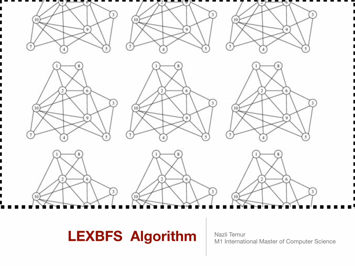
LEXBFS Algorithm Nazli TemurM1 International Master of Computer Science

OUTLINE

Terminology

Chordal Graphs & Properties

LexBFS Intoduction

LexM Introduction

Visualization of Minimal Vertex Separators via LexBFS

Conclusion

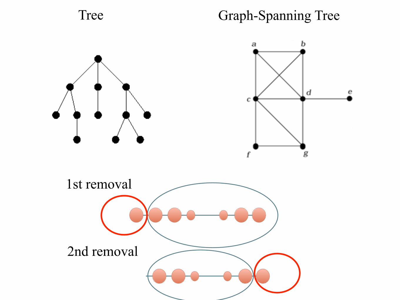
Graph-Spanning TreeTree

1st removal

2nd removal

Cordal Graphs

Definition. A Graph is chordal if it has no induced cycles larger than triangles.

For a graph G on n vertices, the following conditions are equivalent:

G is chordal;

1.G has a perfect elimination ordering. (If every induced subgraph of G has a simplicial vertex)

2. If every minimal vertex separator of a G is complete.

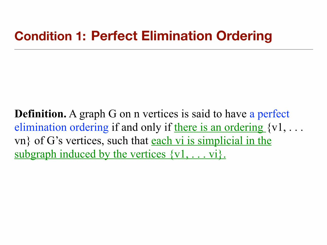
Condition 1: Perfect Elimination Ordering

Definition. A graph G on n vertices is said to have a perfect elimination ordering if and only if there is an ordering {v1, . . . vn} of G’s vertices, such that each vi is simplicial in the subgraph induced by the vertices {v1, . . . vi}.

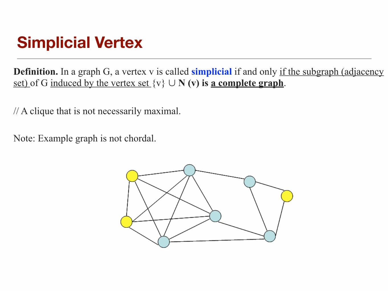
Simplicial VertexDefinition. In a graph G, a vertex v is called simplicial if and only if the subgraph (adjacency set) of G induced by the vertex set {v} ∪ N (v) is a complete graph.

// A clique that is not necessarily maximal.

Note: Example graph is not chordal.

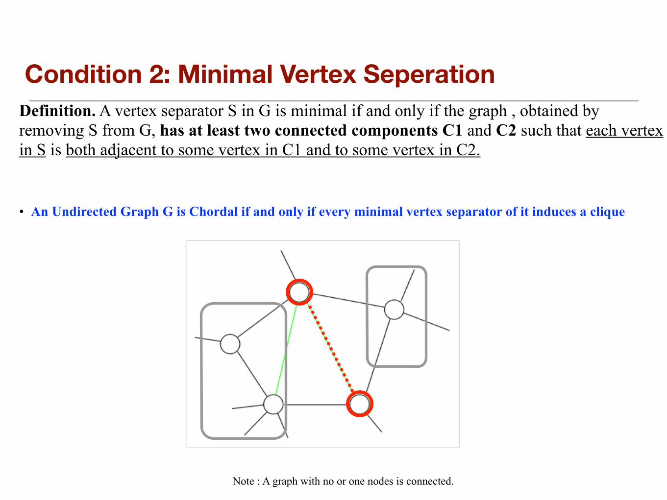
Condition 2: Minimal Vertex SeperationDefinition. A vertex separator S in G is minimal if and only if the graph , obtained by removing S from G, has at least two connected components C1 and C2 such that each vertex in S is both adjacent to some vertex in C1 and to some vertex in C2.

• An Undirected Graph G is Chordal if and only if every minimal vertex separator of it induces a clique

Note : A graph with no or one nodes is connected.

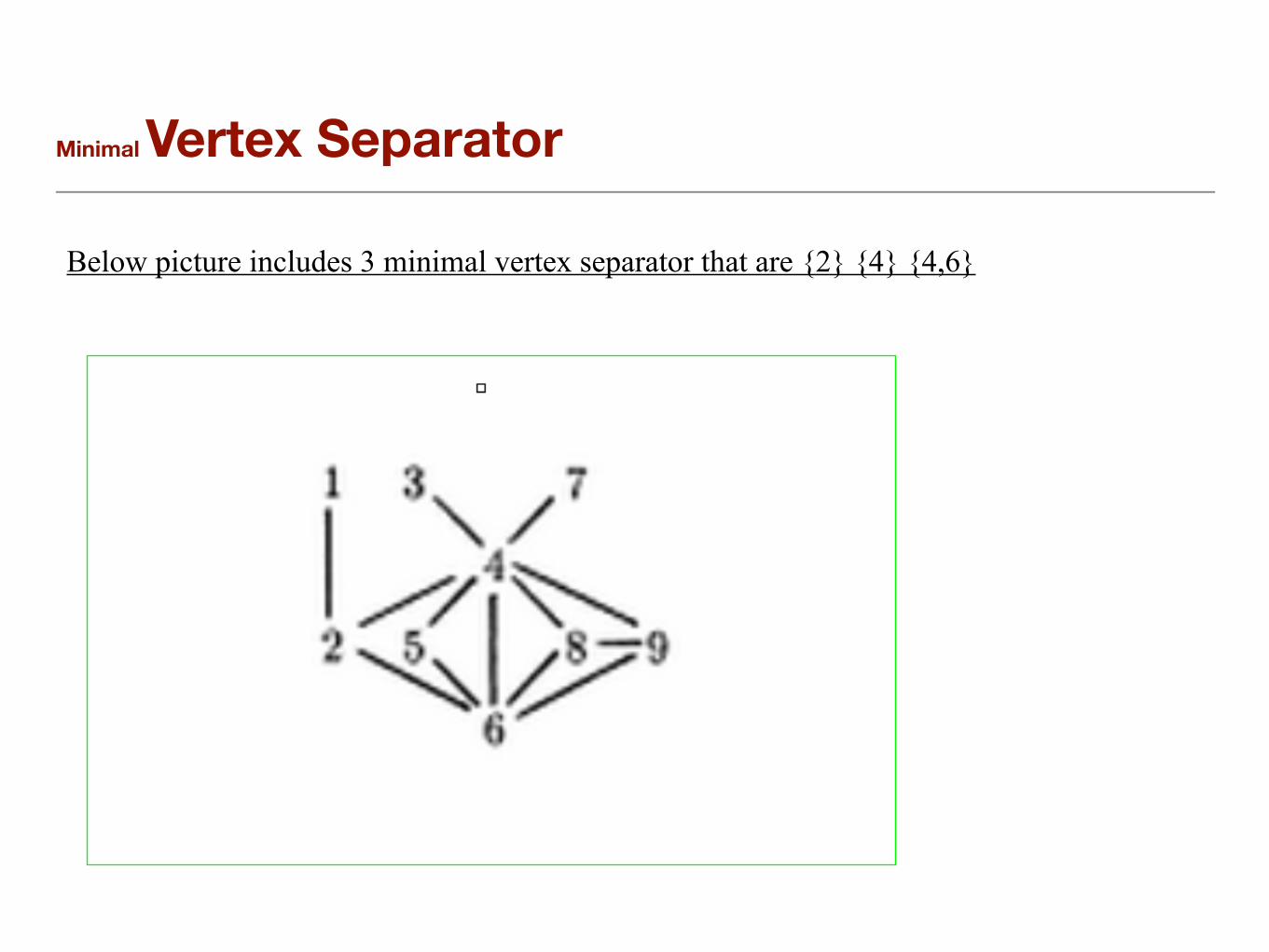
Minimal Vertex Separator

Below picture includes 3 minimal vertex separator that are {2} {4} {4,6}

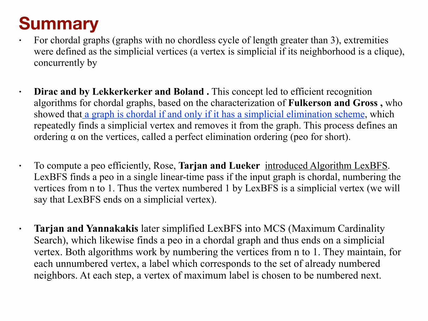
• For chordal graphs (graphs with no chordless cycle of length greater than 3), extremities were defined as the simplicial vertices (a vertex is simplicial if its neighborhood is a clique), concurrently by

• Dirac and by Lekkerkerker and Boland . This concept led to efficient recognition algorithms for chordal graphs, based on the characterization of Fulkerson and Gross , who showed that a graph is chordal if and only if it has a simplicial elimination scheme, which repeatedly finds a simplicial vertex and removes it from the graph. This process defines an ordering α on the vertices, called a perfect elimination ordering (peo for short).

• To compute a peo efficiently, Rose, Tarjan and Lueker introduced Algorithm LexBFS. LexBFS finds a peo in a single linear-time pass if the input graph is chordal, numbering the vertices from n to 1. Thus the vertex numbered 1 by LexBFS is a simplicial vertex (we will say that LexBFS ends on a simplicial vertex).

• Tarjan and Yannakakis later simplified LexBFS into MCS (Maximum Cardinality Search), which likewise finds a peo in a chordal graph and thus ends on a simplicial vertex. Both algorithms work by numbering the vertices from n to 1. They maintain, for each unnumbered vertex, a label which corresponds to the set of already numbered neighbors. At each step, a vertex of maximum label is chosen to be numbered next.

Summary

LEX BFS Intro

Cordal Graph Recognition with LEX BFS

Rose, Lueker & Tarjan (1976) (see also Habib et al. 2000) show that a perfect elimination ordering of a chordal graph may be found efficiently using an algorithm known as lexicographic breadth-first search.

LEX BFS Partition Refinement

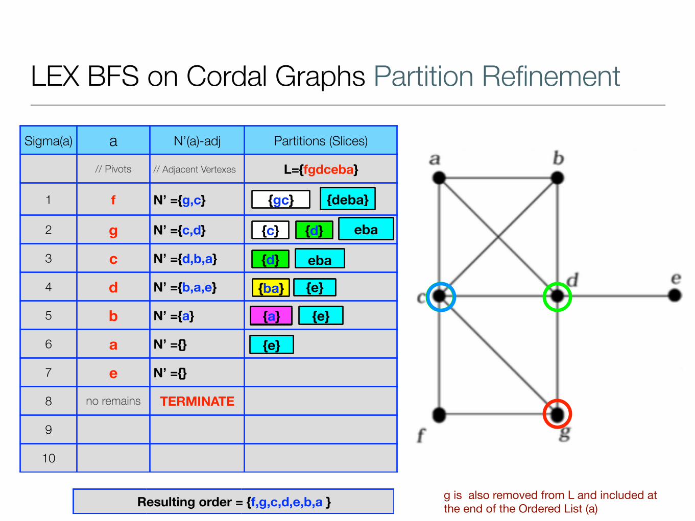
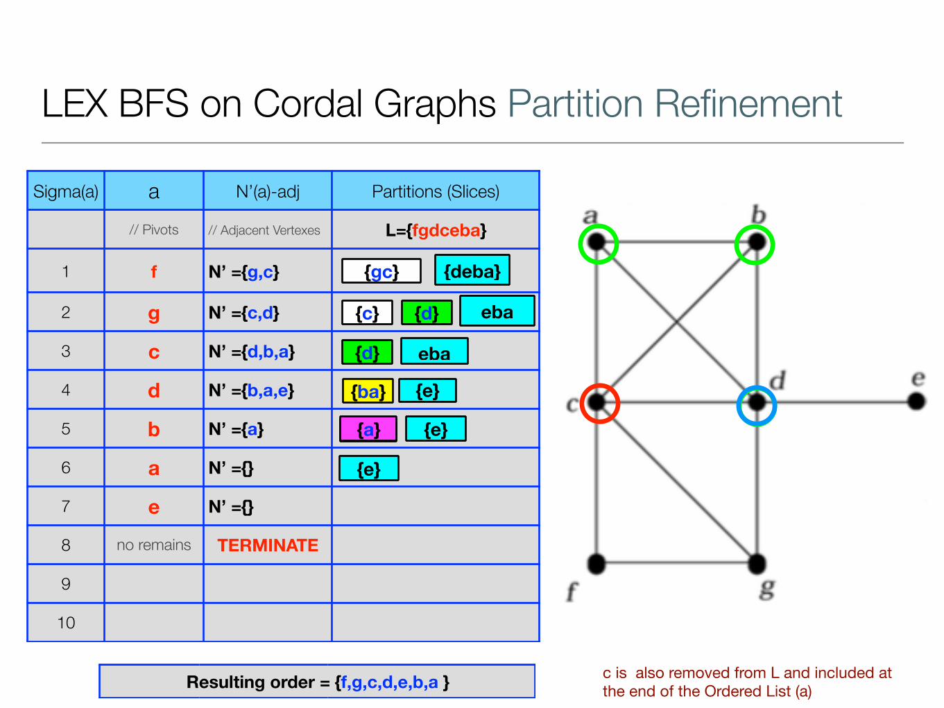
LEX BFS on Cordal Graphs Partition Refinement

Resulting order = {f,g,c,d,e,b,a }

f is removed from L and included at the top of the Ordered List (a)

Sigma(a) a N’(a)-adj Partitions (Slices)

// Pivots // Adjacent Vertexes L={fgdceba}

1 f N’ ={g,c}

2 g N’ ={c,d}

3 c N’ ={d,b,a}

4 d N’ ={b,a,e}

5 b N’ ={a}

6 a N’ ={}

7 e N’ ={}

8 no remains TERMINATE

9

10

{gc} {deba}

{c} eba{d}

{d}

{ba} {e}

{a} {e}

eba

{e}

LEX BFS on Cordal Graphs Partition Refinement

Resulting order = {f,g,c,d,e,b,a } g is also removed from L and included at the end of the Ordered List (a)

Sigma(a) a N’(a)-adj Partitions (Slices)

// Pivots // Adjacent Vertexes L={fgdceba}

1 f N’ ={g,c}

2 g N’ ={c,d}

3 c N’ ={d,b,a}

4 d N’ ={b,a,e}

5 b N’ ={a}

6 a N’ ={}

7 e N’ ={}

8 no remains TERMINATE

9

10

{gc} {deba}

{c} eba{d}

{d}

{ba} {e}

{a} {e}

eba

{e}

LEX BFS on Cordal Graphs Partition Refinement

Resulting order = {f,g,c,d,e,b,a } c is also removed from L and included at the end of the Ordered List (a)

Sigma(a) a N’(a)-adj Partitions (Slices)

// Pivots // Adjacent Vertexes L={fgdceba}

1 f N’ ={g,c}

2 g N’ ={c,d}

3 c N’ ={d,b,a}

4 d N’ ={b,a,e}

5 b N’ ={a}

6 a N’ ={}

7 e N’ ={}

8 no remains TERMINATE

9

10

{gc} {deba}

{c} eba{d}

{d}

{ba} {e}

{a} {e}

eba

{e}

LEX BFS on Cordal Graphs Partition Refinement

Sigma(a) a N’(a)-adj Partitions (Slices)

// Pivots // Adjacent Vertexes L={fgdceba}

1 f N’ ={g,c}

2 g N’ ={c,d}

3 c N’ ={d,b,a}

4 d N’ ={b,a,e}

5 b N’ ={a}

6 a N’ ={}

7 e N’ ={}

8 no remains TERMINATE

9

10

{gc} {deba}

{c} eba{d}

Resulting order = {f,g,c,d,b,a,e }

{d}

{ba} {e}

{a} {e}

eba

d is also removed from L and included at the end of the Ordered List (a)

{e}

LEX BFS on Cordal Graphs Partition Refinement

Resulting order = {f,g,c,d,e,b,a } b is also removed from L and included at the end of the Ordered List (a)

Sigma(a) a N’(a)-adj Partitions (Slices)

// Pivots // Adjacent Vertexes L={fgdceba}

1 f N’ ={g,c}

2 g N’ ={c,d}

3 c N’ ={d,b,a}

4 d N’ ={b,a,e}

5 b N’ ={a}

6 a N’ ={}

7 e N’ ={}

8 no remains TERMINATE

9

10

{gc} {deba}

{c} eba{d}

{d}

{ba} {e}

{a} {e}

eba

{e}

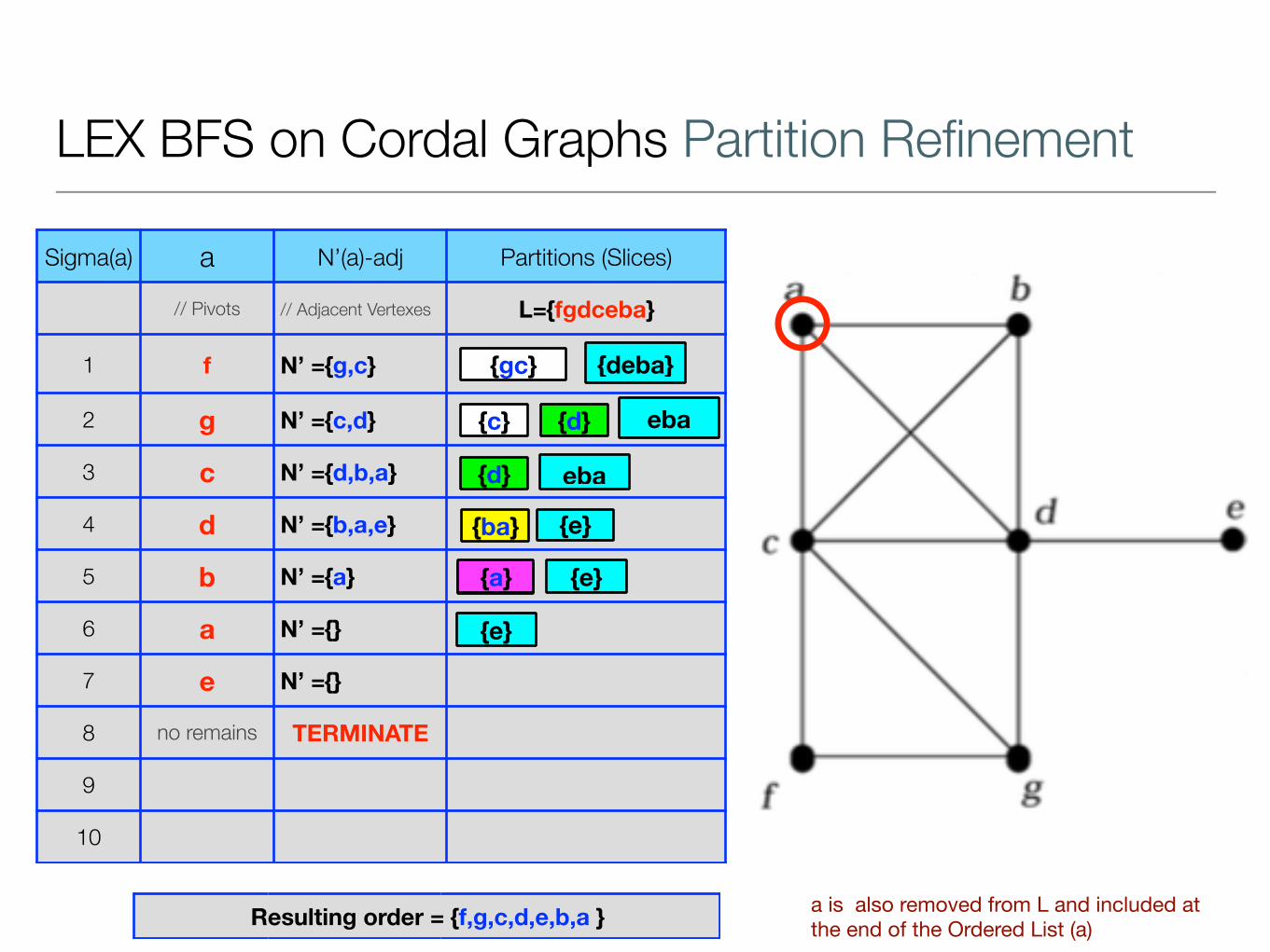
LEX BFS on Cordal Graphs Partition Refinement

Resulting order = {f,g,c,d,e,b,a } a is also removed from L and included at the end of the Ordered List (a)

Sigma(a) a N’(a)-adj Partitions (Slices)

// Pivots // Adjacent Vertexes L={fgdceba}

1 f N’ ={g,c}

2 g N’ ={c,d}

3 c N’ ={d,b,a}

4 d N’ ={b,a,e}

5 b N’ ={a}

6 a N’ ={}

7 e N’ ={}

8 no remains TERMINATE

9

10

{gc} {deba}

{c} eba{d}

{d}

{ba} {e}

{a} {e}

eba

{e}

LEX BFS on Cordal Graphs Partition Refinement

Resulting order = {f,g,c,d,e,b,a } e is also removed from L and included at the end of the Ordered List (a)

Sigma(a) a N’(a)-adj Partitions (Slices)

// Pivots // Adjacent Vertexes L={fgdceba}

1 f N’ ={g,c}

2 g N’ ={c,d}

3 c N’ ={d,b,a}

4 d N’ ={b,a,e}

5 b N’ ={a}

6 a N’ ={}

7 e N’ ={}

8 no remains TERMINATE

9

10

{gc} {deba}

{c} eba{d}

{d}

{ba} {e}

{a} {e}

eba

{e}

LEX-M

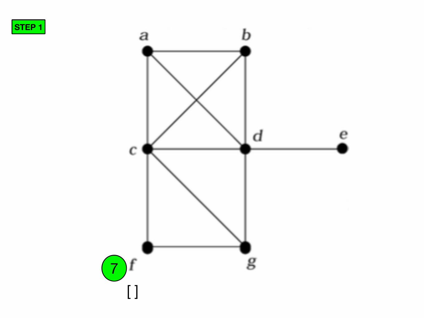
STEP 1

[ ]7

[ ]7

[7,]

[7,]

STEP 2

[ ]7 6

[7]

[7,]

STEP 3

[ ]7 6

[7]

[7,6] [6,]

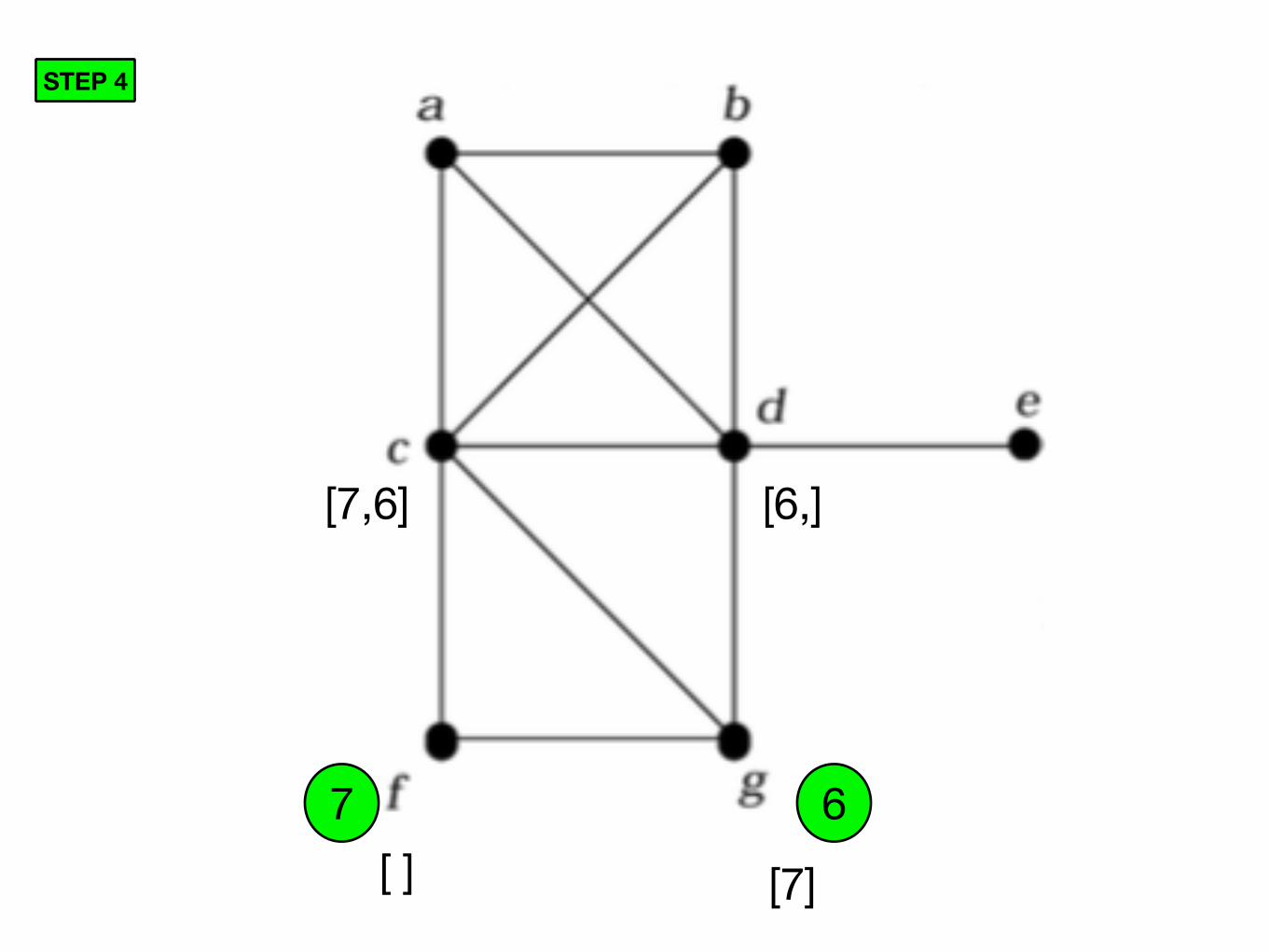
STEP 4

[ ]7 6

[7]

[7,6] [6,]5

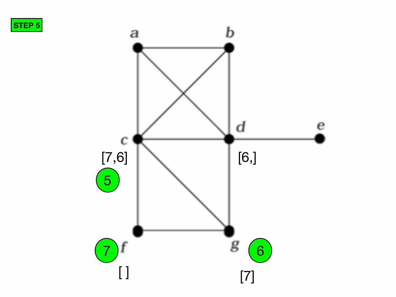
STEP 5

[ ]7 6

[7]

[7,6] [6,5]5

[5,] [5,]

STEP 6

[ ]7 6

[7]

[7,6] [6,5]5

[5,] [5,]

4

STEP 7

[ ]7 6

[7]

[7,6] [6,5]5

[5,4,] [5,4,]

4

[4]

STEP 8

[ ]7 6

[7]

[7,6] [6,5]5

[5,4,] [5,4,]

4

[4]

3

STEP 9

[ ]7 6

[7]

[7,6] [6,5]5

[5,4,3,] [5,4]

4

[4]

3

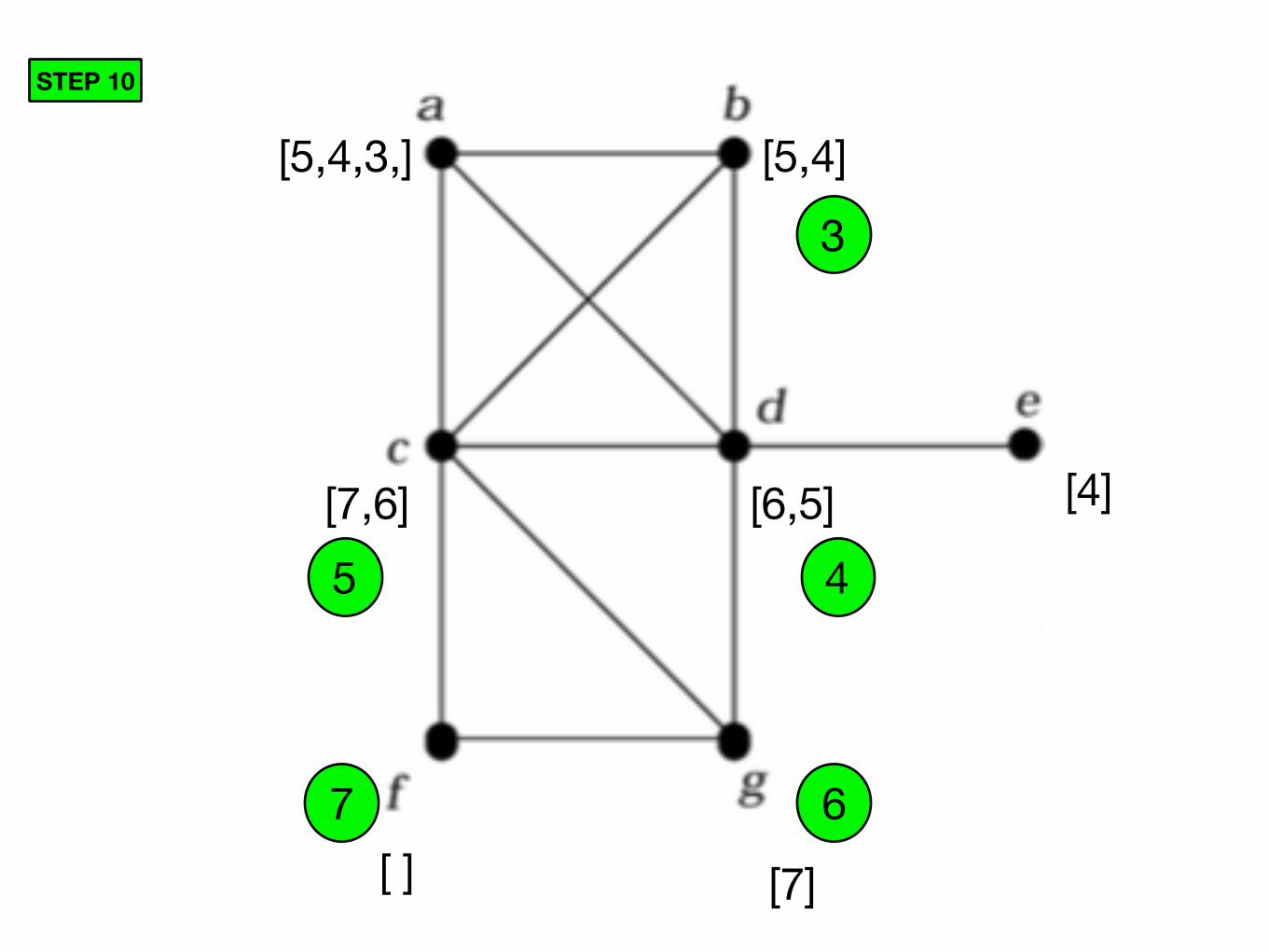
STEP 10

[ ]7 6

[7]

[7,6] [6,5]5

[5,4,3,] [5,4]

4

[4]

3

STEP 11

2

[ ]7 6

[7]

[7,6] [6,5]5

[5,4,3] [5,4]

4

[4]

3

STEP 12

2

1

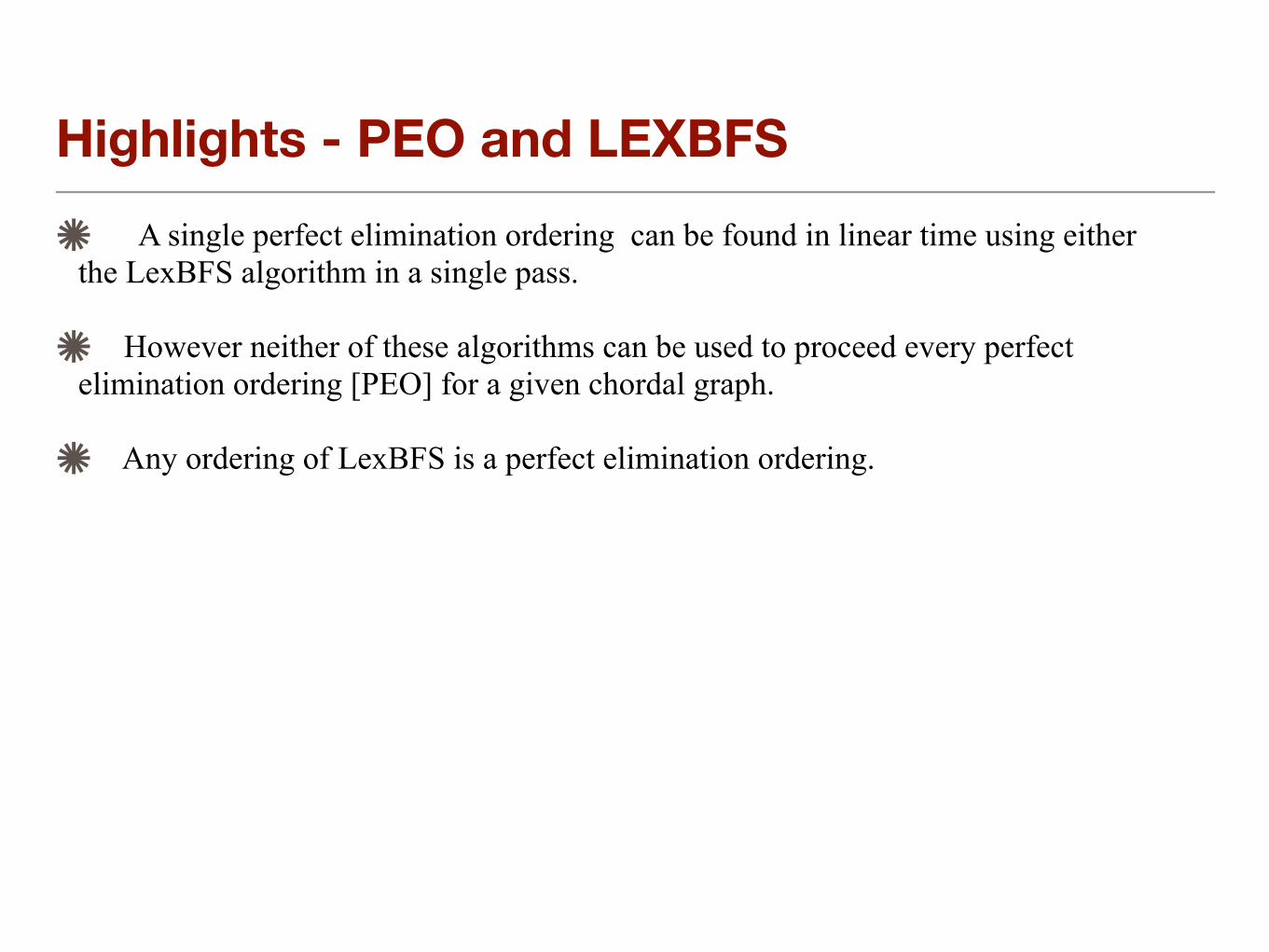
Highlights - PEO and LEXBFS A single perfect elimination ordering can be found in linear time using either

the LexBFS algorithm in a single pass.

However neither of these algorithms can be used to proceed every perfect elimination ordering [PEO] for a given chordal graph.

Any ordering of LexBFS is a perfect elimination ordering.

Minimal Vertex Separators

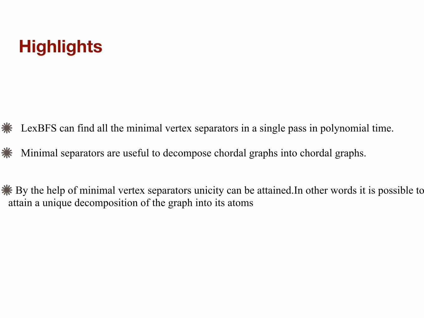
LexBFS can find all the minimal vertex separators in a single pass in polynomial time.

Minimal separators are useful to decompose chordal graphs into chordal graphs.

By the help of minimal vertex separators unicity can be attained.In other words it is possible to attain a unique decomposition of the graph into its atoms

Highlights

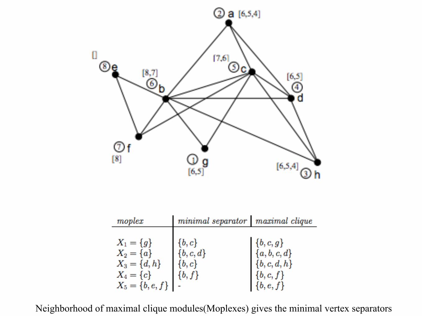
Neighborhood of maximal clique modules(Moplexes) gives the minimal vertex separators

LEX-BFS outputs the same ordering as BFS ..

BFS Path

f

g c

d b a

Resulting order = {f }

e

1

BFS Path

f

g c

d b a

Resulting order = {f,g}

e

1

2

BFS Path

f

g c

d b a

Resulting order = {f,g,c }

e

12

3

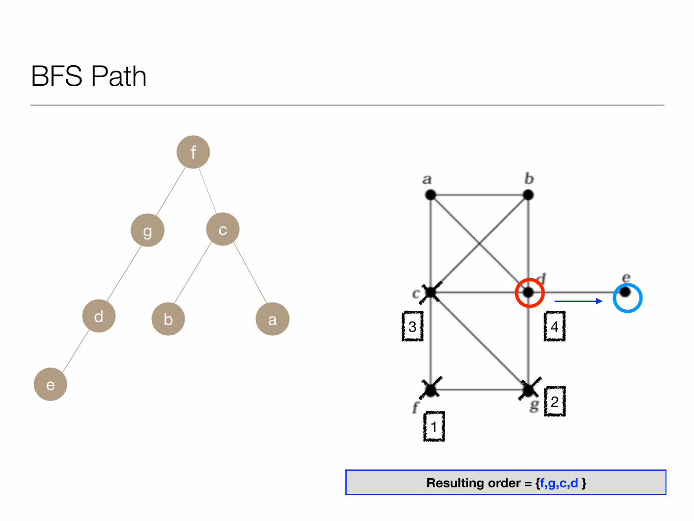
BFS Path

f

g c

d b a

Resulting order = {f,g,c,d }

e

12

3 4

BFS Path

f

g c

d b a

Resulting order = {f,g,c,d,b }

e

12

3

5

4

BFS Path

f

g c

d b a

Resulting order = {f,g,c,d,b,a }

e

12

3 4

56

BFS Path

f

g c

d b a

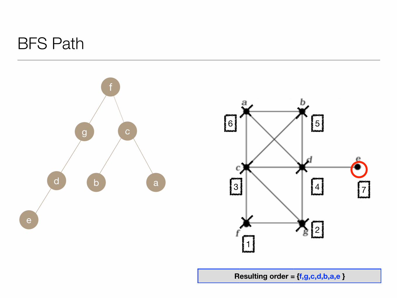
Resulting order = {f,g,c,d,b,a,e }

e

12

3 4

56

7

BFS Path

f

g c

d b a

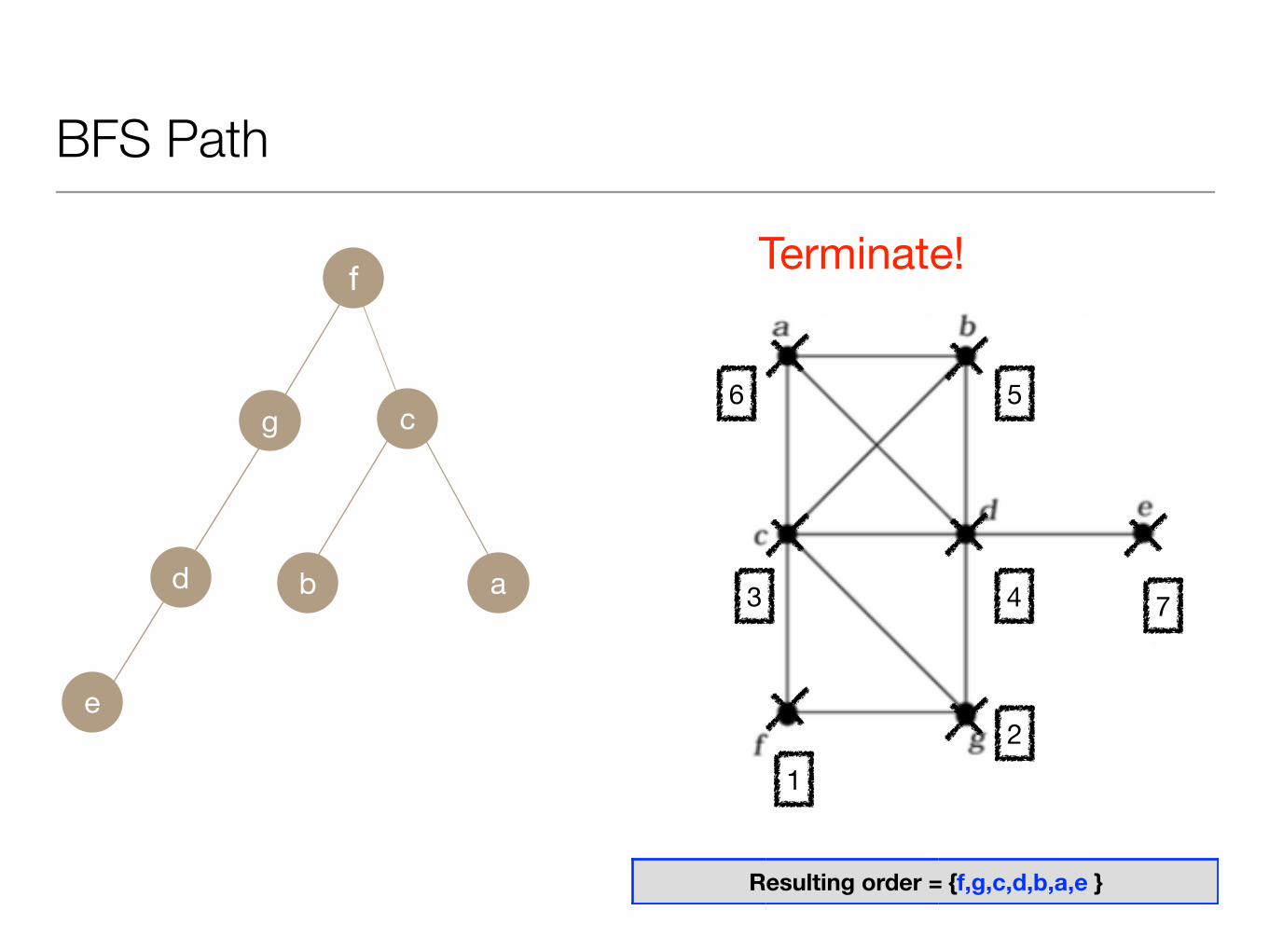
Resulting order = {f,g,c,d,b,a,e }

e

12

3 4

56

7

Terminate!

CONCLUSIONIn this research what I tried to obtain was the answers of those questions. What is LEXBFS Algorithm? How it is designed ? What was the need ? What are the appliances ? So now we can conclude as LexBFS Algorithm is an algorithm that is mainly proposed for Chordal/Triangulated Graph Recognition. LexBFS can give us the answers of if 3 main property is satisfied of not(Induced subgraph is also a Chordal, It satisfies Perfect Elimination Ordering Schema and The Minimal Vertex Separator induces a clique.)LexBFS has many variations and it is applied also for many other graph recognition via Minimal Vertex Separator Clique Characterization. Also By adding some more constraints instead or breaking ties arbitrarily.We can obtain additional restricted orderings that can serve for the solution of a sub problem domain.This algorithm is a very strong algorithm that attracts the attention of many researchers because of its simplicity efficiency and customizability.The main focus was the appliances of LEXBFS for Finding Minimal Vertex Separators. In this focus area we have reached the answers of LEXBFS can generate all the MVSs via Moplex Elimination ordering efficiently. In addition to this. The way it process is passing through connected components C1 C3… , Unique GraphDecomposition (Atomicity),Graph Triangulation topics can be supported indirectly via LEXBFS and directly via Minimal Vertex Separators. The appliances that are related to chordal graphs are ;Elimination Trees,Equivalent Orderings,Re-ordering for Stack Storage Reduction,Partitioning for Parallel Triangular Solution.Clique Trees and Multifraontal Method,Ordering Heuristics, Jess and Kees Orderings , a Block Jess and Kees Re-orderings.

THANKS !