This paper presents preliminary findings and is being distributed to economists

and other interested readers solely to stimulate discussion and elicit comments.

The views expressed in this paper are those of the authors and do not necessarily

reflect the position of the Federal Reserve Bank of New York or the Federal

Reserve System. Any errors or omissions are the responsibility of the authors.

Federal Reserve Bank of New York

Staff Reports

Leverage Limits and Bank Risk:

New Evidence on an Old Question

Dong Beom Choi

Michael R. Holcomb

Donald P. Morgan

Staff Report No. 856

June 2018

Leverage Limits and Bank Risk: New Evidence on an Old Question

Dong Beom Choi, Michael R. Holcomb, and Donald P. Morgan

Federal Reserve Bank of New York Staff Reports, no. 856

June 2018

JEL classification: G20, G21, G28

Abstract

The supplementary leverage ratio (SLR) rule recently imposed on the very largest U.S. banks has

revived the question of whether banks sidestep such rules by shifting toward riskier, higher-

yielding assets. Using difference-in-difference analysis, we find that, after the SLR was finalized

in 2014, covered banks shifted their portfolio toward riskier (risk-weighted) assets and higher-

yielding securities compared to other large banks not subject to the rule. The shifts are sizable and

tend to be larger at banks more constrained ex ante by the leverage limit. Despite increased asset

risk, overall bank risk (book and market measures) did not increase, suggesting the higher capital

required under the new rule offset the risk-shifting. Taken together, our findings reinforce

regulators’ long-standing concerns about risk-shifting around leverage limits and suggest that the

recent recalibration will curb those incentives without necessarily increasing bank risk.

Key words: Basel III regulation, bank risk, leverage limit, regulatory arbitrage, reaching for yield

_________________

Choi, Holcomb, Morgan (corresponding author): Federal Reserve Bank of New York (email: don.morgan@ny.frb.org). The authors thank Davy Perlman, Ulysses Velasquez, and Elaine Yao for helpful research assistance. The views expressed in this paper are those of the authors and do not necessarily reflect the position of the Federal Reserve Bank of New York or the Federal Reserve System. To view the authors’ disclosure statements, visit https://www.newyorkfed.org/research/staff_reports/sr856.html.

1

Because our existing capital standards treat all bank assets alike, they have had the effect of encouraging some institutions to scale back their holdings of relatively liquid, low-risk assets (Paul Volker, 1987) …a leverage requirement that is too high favors high-risk activities and disincentivizes low-risk activities (Randal K. Quarles, 2018)

I. Introduction

The quotes above illustrate the déjà vu aspect of our question. The first is Fed Chairman

Volker explaining to Congress why bank regulators were moving from the leverage rule imposed

in 1981 to more risk-based capital rules. The second is the current Fed Vice Chairman for

Supervision explaining why the new leverage rule that took effect this year was being

recalibrated to curb risk-shifting incentives. Bankers, for their part, have also warned the new

rule could have unintended effects:

… the proposal would have discouraged banks from holding low-yielding, high-quality assets…in preference for riskier assets which would produce a higher relative return of capital. (J.P. Morgan (2014))

Despite these long-standing and widely held concerns, published evidence for the risk-

shifting conjecture is relatively scarce. The leverage rule imposed in 1981 motivated several

theoretical papers predicting potentially perverse consequences (Koehn and Santomero (1980),

Kim and Santomero (1988)), but Furlong (1988) seems to be the only empirical test and finds

evidence that contradicts the theoretical conjectures. The paucity of evidence from that first

experiment might reflect the fact that the first leverage rule covered all banks and was rarely

binding, making a plausible control group difficult to identify. By contrast, the Supplementary

Leverage Ratio (SLR) covers only the very largest U.S. banks, and for some, may bind more

than their risk-based capital limit. Thus, this latest leverage rule “experiment” provides a better

setting to test the risk-shifting conjecture.

We look for evidence of risk-shifting around the new leverage rule using difference-in-

difference analysis. Our treated group comprises the 15 bank holding companies (“banks”)

subject to the new rule, the so-called “advanced approach” firms that use internally generated

2

risk estimates for setting their risk-based capital requirements. Concerns that these firms might

be underestimating risk and overstating their risk-based capital strength motivated the new

leverage ratio as a supplement or back stop (Basel Committee on Banking Supervision 2009).2

Advance approach firms, by definition, are very large; at least $250 billion in total assets or $10

billion in foreign exposures. Our control group comprises the 18 banks with assets between $50

and $250 billion not covered by the new rule. Though smaller, these banks are officially large

per the Dodd-Frank Act of 2010 and thus face similar regulatory environments apart from the

SLR. Using standard difference-in-difference regressions with time and institution fixed effects

and a parsimonious set of controls (including lagged risk-based capital ratios), we compare

various risk measures before and after the SLR was finalized in September 2014.

We study risk three ways. We first look directly at banks’ risk-weighted asset shares

using Basel risk-weighting classifications. The validity of that measure hinges, of course, on the

accuracy of banks’ risk weights and it was doubts surrounding those that motivated the new rule

in the first place. Our second measure, security yields, is independent of reported risks. We

gathered banks’ individual security holdings from the confidential regulatory filings then

matched with yields from a variety of sources. If leverage-constrained banks are shedding safer

assets and “reaching for yield” on riskier ones, it should register in these data even if obscured

by errors in reported, risk-weighted assets. Lastly, we look at measures of overall bank risk.

Even if covered banks are shifting to riskier assets, they may not be riskier overall if they are less

levered than they would have been otherwise. The overall risk measures we examine, both book

and market, capture the combined effect of any risk-shifting and reduced leverage.

Our findings are largely consistent with the risk-shifting conjecture. Risk weighted assets

at covered banks have increased particularly at banks for which the leverage constraint is tighter.

We detect the shift in securities and trading assets, but not loans, which seems sensible as loans

are arguably the least adjustable asset class. Consistent with “reach for yield” concerns, we find

a sizable, about 30 basis point, increase in the average yield on securities held by covered banks;

we also find suggestive evidence that this gain reflects banks actively adding riskier securities to

their portfolio, not merely shedding safer ones.

Despite the evident risk-shifting, we find no increase in the battery of overall bank risk

measures we examine, including Z scores, CDS spreads, equity volatility, and others, not even 2 See Santos and Plosser (2016) for evidence and references.

3

for the most constrained banks. This suggests the higher capital required by the new rule offsets

the risk-shifting, or vice-versa. In fact, we show that leverage ratio at the most constrained banks

rose sharply in relative and absolute terms post-implementation.

While others have already “leveraged” the new leverage rule for research purposes, we

are the first to study its effects at the overall portfolio and bank risk level for U.S. banks. The

other recent literature focuses on narrower segments, the repurchase (repo) market in particular.3

Allahrakha et al. (2016) find that U.S. banks decreased repo borrowing in response the SLR rule

introduced and, consistent with our finding, shifted toward more volatile collateral. Bicu et al

(2017) find reduced liquidity in the U.K. repo after a related leverage limit was announced there.

By contrast, Bucalossi and Scalia (2016) find that leverage-constrained European banks did not

reduce their repo volumes between 2013 and 2014.4 The paper closest to ours, Acosta Smith et

al. (2017), detects a shift toward riskier assets by European banks in response to a leverage rule

proposal by the Basel committee, but no increase in overall risk, consistent with our findings.

On the policy front, our findings suggest that that recalibrating the new leverage ratio to

minimize risk-shifting incentives will not increase bank risk.5

Section II reviews the history of leverage limits in the U.S., from the first in 1981 to the

latest. Section III discusses our empirical strategy and potential confounding regulatory changes.

Section IV describes our data and results for risk-weighted asset shares, securities yields, and

overall risk measures. Section V concludes.

II. From Leverage Limits and Back Again

We trace the circle of capital regulation over the last 40 years from leverage limits to

risk-based capital rules, then back, partly, to leverage limits.

Concerned about rising failures and falling capital levels across the banking system, U.S.

bank regulators announced explicit, uniform capital ratio requirements for the first time in 1981

3 Becker and Ivashina (2015) find evidence of somewhat different form regulatory arbitrage by insurance companies; within credit rating categories, insurance firms tend to shift toward riskier securities. Ellul et al. (2014) study how accounting rules, through the interaction with capital regulations, affect risk-taking of insurance companies. 4 Boyarchenko et al. (2017) attribute recent illiquidity in the corporate bond and credit default swap markets to a binding leverage limit. 5 https://www.federalreserve.gov/newsevents/pressreleases/bcreg20180411a.htm

4

(Volker 1987).6 Capital adequacy before that was assessed bank-by-bank per supervisors so the

shift to formal standards marked an important shift in regulatory policy. The rules required at

least 5.5 percent primary capital and 6 percent total capital relative to total, on balance sheet

assets. While the capital requirements were conditional on capital quality, they were invariant to

asset risk so they were in effect leverage limits.

That first leverage rule spurred a debate on whether, as a theoretical matter, it might

actually increase bank risk via asset substitution (Koehn and Santomero (1980), Kim and

Santomero (1988), Furlong and Keeley (1989)). The only empirical test of that question at the

time appears to be Furlong (1988). Starting with 98 large, public banks, he compares changes in

three risk measures between 1981 and 1986 for 24 “capital deficient” banks in 1981 per the new

standards and 75 that were “capital sufficient” banks. Contrary to the risk-shifting hypothesis, he

finds no significant differential changes in the market-based asset risk measure he constructs or

in bank default risk (Z) scores. He does document a relative decline in the ratio of low-risk,

liquid assets at the capital deficient banks but that trend began, as he notes, well before the

capital rules were introduced.

Lingering concerns about unintended leverage rule effects led the Federal Reserve in

1986 to propose replacing it with risk-based capital requirements based on total assets, including

off-balance sheet assets (Volker 1987, Wall 1989). That proposal, in cooperation with

international bank regulators, evolved into the Basel I capital accord in 1990. Basel I defined

standard risk weights for broad asset classes and set required capital minimums relative to risk-

weighted assets. That change curbed incentives under the leverage rule to shift toward riskier

categories, though not necessarily within the fairly broad asset classes defined under Basel I.

Basel II in 2004 elaborated more risk-sensitive capital requirements and allowed very large,

“advanced approach” firms the option of using internal models to estimate asset risk (subject to

supervisory review).

Concerns that advanced approach firms might be underestimating risk and exaggerating

their capital strength, as well as the 2007-2008 financial crisis, led to the (partial) return of

leverage ratios (see Figure 1 below). The Basel Committee recommended a leverage rule (the

Basel III leverage ratio) in 2010 and U.S. regulators proposed their version—the Supplementary

6 Regulators could still require higher capital at banks with substantial off-balance-sheet exposures or assets considered particularly risky (Gilbert et al. 1985, p. 16)

5

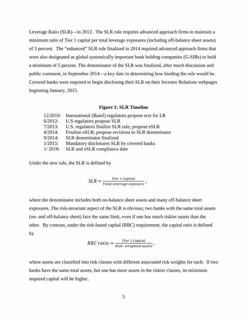
Leverage Ratio (SLR)—in 2012. The SLR rule requires advanced approach firms to maintain a

minimum ratio of Tier 1 capital per total leverage exposures (including off-balance sheet assets)

of 3 percent. The “enhanced” SLR rule finalized in 2014 required advanced approach firms that

were also designated as global systemically important bank holding companies (G-SIBs) to hold

a minimum of 5 percent. The denominator of the SLR was finalized, after much discussion and

public comment, in September 2014—a key date in determining how binding the rule would be.

Covered banks were required to begin disclosing their SLR on their Investor Relations webpages

beginning January, 2015.

Figure 1: SLR Timeline

12/2010: International (Basel) regulators propose text for LR 6/2012: U.S regulators propose SLR 7/2013: U.S. regulators finalize SLR rule; propose eSLR 4/2014: Finalize eSLR; propose revisions to SLR denominator 9/2014: SLR denominator finalized 1/2015: Mandatory disclosures SLR by covered banks 1/ 2018: SLR and eSLR compliance date

Under the new rule, the SLR is defined by

SLR = 𝑇𝑇𝑇𝑇𝑇𝑇𝑇𝑇 1 𝐶𝐶𝐶𝐶𝐶𝐶𝑇𝑇𝐶𝐶𝐶𝐶𝐶𝐶𝑇𝑇𝑇𝑇𝐶𝐶𝐶𝐶𝐶𝐶 𝐶𝐶𝑇𝑇𝑙𝑙𝑇𝑇𝑇𝑇𝐶𝐶𝑙𝑙𝑇𝑇 𝑇𝑇𝑒𝑒𝐶𝐶𝑇𝑇𝑒𝑒𝑒𝑒𝑇𝑇𝑇𝑇

,

where the denominator includes both on-balance sheet assets and many off-balance sheet

exposures. The risk-invariant aspect of the SLR is obvious; two banks with the same total assets

(on- and off-balance sheet) face the same limit, even if one has much riskier assets than the

other. By contrast, under the risk-based capital (RBC) requirement, the capital ratio is defined

by

𝑅𝑅𝑅𝑅𝑅𝑅 𝑟𝑟𝑟𝑟𝑟𝑟𝑟𝑟𝑟𝑟 = 𝑇𝑇𝑇𝑇𝑇𝑇𝑇𝑇 1 𝐶𝐶𝐶𝐶𝐶𝐶𝑇𝑇𝐶𝐶𝐶𝐶𝐶𝐶𝑅𝑅𝑇𝑇𝑒𝑒𝑅𝑅−𝑤𝑤𝑇𝑇𝑇𝑇𝑙𝑙ℎ𝐶𝐶𝑇𝑇𝑡𝑡 𝐶𝐶𝑒𝑒𝑒𝑒𝑇𝑇𝐶𝐶𝑒𝑒

,

where assets are classified into risk classes with different associated risk weights for each. If two

banks have the same total assets, but one has more assets in the riskier classes, its minimum

required capital will be higher.

6

It was widely reported that the new leverage limits incorporating off-balance sheet

exposures were more binding than the RBC limits for many covered banks (J.P Morgan 2014).

Figure 2 suggests this was in fact the case; among the SLR banks in 2013:Q4, even the most

constrained bank had two percentage points of slack relative to its risk-based capital requirement,

while eight had slack of less than two percentage points relative to their leverage requirement

and six had negative slack.7

Banks bound by the SLR limit have two options: increase tier 1 capital or decrease the

total leverage exposures. If a bank chooses to raise more (costly) capital, one way to offset the

increased costs is by shifting from safer, lower-yielding assets to riskier, higher-yielding ones. If

it instead chooses to reduce its assets, the least costly way to do so would be by shedding assets

with low yields, such as reserves. In both cases, the bank’s share of risky assets relative to safe

assets, and its average yield on assets, should rise.

III. Empirical Strategy

We test for risk shifting by SLR banks using difference-in-difference (DD) regressions:

𝜎𝜎𝑇𝑇𝐶𝐶 = 𝛼𝛼𝑇𝑇 + 𝛼𝛼𝐶𝐶 + 𝛽𝛽 ∗ 𝑆𝑆𝑆𝑆𝑅𝑅𝑇𝑇 + ϒ ∗ 𝑝𝑝𝑟𝑟𝑝𝑝𝑟𝑟𝐶𝐶 + 𝛿𝛿 ∗ 𝑆𝑆𝑆𝑆𝑅𝑅𝑇𝑇 ∗ 𝑝𝑝𝑟𝑟𝑝𝑝𝑟𝑟𝐶𝐶 + 𝛾𝛾 ∗ 𝑅𝑅𝑇𝑇𝐶𝐶−1 + 𝜀𝜀𝑇𝑇𝐶𝐶. (1)

𝜎𝜎𝑇𝑇𝐶𝐶 is one of several risk measures for bank i at t (described below). The firm fixed effect (𝛼𝛼𝑇𝑇)

controls for constant risk differences across banks while the year-quarter fixed effect (𝛼𝛼𝐶𝐶)

controls for time-varying aggregate factors (macro, financial, or monetary) that might affect bank

risk. 𝑆𝑆𝑆𝑆𝑅𝑅𝑇𝑇 equals 1 for banks subject to the rule and 0 otherwise; 𝑝𝑝𝑟𝑟𝑝𝑝𝑟𝑟𝐶𝐶 equals 1 on and after the

SLR treatment date (2014:Q3) and 0 before. The coefficient on SLR*post measures the DD

effect, i.e. how much the difference in risk (SLR banks minus non-SLR banks) differed before

and after the SLR treatment. The risk-shifting hypothesis implies 𝛿𝛿 > 0.

𝑅𝑅𝑇𝑇𝐶𝐶−1 denotes two lagged controls. The first is a proxy for exposure to the new liquidity

coverage rule (LCR) imposed at the same time and on the same banks (to different degrees) as

7 We calculate the SLR for dates before public disclosure using the “total exposures” field of the FR Y-15. We use 2013:Q4 (instead of 2014:Q2) because the data are only available year-end.

7

the SLR.8 The liquidity rule requires banks to hold a minimum share of “high quality liquid

assets” to cover unexpected cash outflows. Since such assets are usually safer as well, the

liquidity rule could prevent banks from shifting toward risker assets in order to circumvent the

leverage rule, thereby attenuating our estimates of the leverage rule effect.9 As banks do not

disclose LCR ratios in their public regulatory filings, as a proxy we use the inverse of the

liquidity stress ratio calculated at the Federal Reserve Bank of New York.10

The second control is the risk-based capital ratio for bank i. Risk-shifting around the

leverage ratio will tend to reduce banks’ risk-based capital ratio (if the shift is detected), hence

all else equal, banks with higher risk-based capital ratios will have more room to maneuver

around the leverage limit.

Identifying the appropriate treatment date for the SLR is not obvious given its roughly six

year gestation period. The compliance date (January 2018) might seem like the natural treatment

date, but banks almost certainly began adjusting before then to ensure a smooth “glide path”

toward public disclosure in 2015 and compliance in 2018.11 The issuance of the final rule in July

2013 is another potential treatment date, except the rule was not literally final; it was followed by 8 The LCR was finalized by U.S. regulators in 2014:Q3 with phase in starting 2015:Q1. The rule covers all banks in our sample, but the SLR banks face a stricter rule. https://www.federalreserve.gov/newsevents/pressreleases/bcreg20140903a.htm. 9 Another confounding regulation is the “accumulated other comprehensive income” (AOCI) rule which may also, like the LCR, induce covered banks to shift toward safer assets. The AOCI rule mostly affects our treatment group of SLR-covered banks, with similar treatment dates as well. Again, the direction of its impact on bank risk-taking is the opposite of the SLR, thus attenuating our estimates. 10 The liquidity stress ratio (LSR), our proxy for the LCR calculated by the NY Fed Research, is defined as LSR = potential liquidity inflow

potential liquidity outflow= liquidity adjusted assets

liquidity adjusted liabilities and off balance sheet exposures.

The liquidity adjustments reflect the estimated run-risk of each liability type or off balance sheet exposure. Adjusted liabilities grow when the expected funding outflow is higher, as in stressful times, while adjusted assets shrink when the expected price decline is greater in a market illiquidity event. Thus, a bank is more exposed to liquidity risks if its LSR is higher. The liquidity adjustment used in the LSR follow LCR assumptions when possible, but since the LSR is based on only public information, some differences are possible. We use the inverse of LSR to approximate historical LCR. For more discussion, see Choi and Zhou (2016). 11 Anecdotally, banks were already adjusting in anticipation of the public disclosures in January 2015: Bank of New York Mellon (https://www.bnymellon.com/_global-assets/pdf/our-thinking/arriving-at-new-capital-ratios.pdf) reports that the “…banking organizations are already making changes to comply with the SLR given that the final rules require public disclosures beginning January 1, 2015.” A recent Bloomberg article (https://www.bloomberg.com/news/articles/2018-02-01/deposit-shunning-banks-get-big-break-as-u-s-eases-leverage-rule) reports that “The U.S. gold-plated the Basel leverage requirement for the eight largest lenders when it implemented its own version in 2014, … The next year, BNY Mellon was still below the 5 percent minimum and State Street barely above. That prompted them to push away deposits with measures that included additional fees on certain types of accounts. They also switched how they swept institutional clients’ extra cash, moving them into money-market funds instead of regular deposits.”

8

consultations with the banking industry which offered many suggestions for refining, i.e.

shrinking, the denominator. Regulators incorporated some, but not others (e.g. excluding cash

and central bank reserves), leading to the revised denominator in September 2014. Only after that

date would banks know how the denominator would be calculated, and thus, how constraining

the SLR would be.

IV. Data and Findings

We look first at risk-weighted asset shares, then securities yields, then overall risk measures.

a. Risk-Weighted Assets Shares

Risk-weighted assets are reported by bank holding companies in their quarterly reports

to bank regulators (FR Y-9C, Schedule HC-R Part II). Reporting standards changed in 2015:Q1,

when banks commenced reporting risk-weighted assets according to Basel III definitions. To

ensure a consistent series, we adjusted the risk weightings after 2015:Q1 to approximate those

before (see Appendix for details). As a precaution, we report results using adjusted and

unadjusted weightings; our results are similar for both.

Table 1 reports sample statistics for risk-weighted (RW) asset shares for the SLR banks

and non-SLR banks both pre-treatment (2011:Q1-2014:Q2) and post-treatment (2014:Q3-

2016:Q2).12 We look at RW assets overall, and by broad asset class: securities, trading assets,

and loans.13 We expect any risk shifting to be more apparent for securities and trading assets as

they are typically more liquid and thus easier to adjust than loans.14 The unconditional

difference-in-difference (DD), reported in Column 5, is positive and significant for RW total

assets, securities, and trading assets. The unconditional DD for loans is much smaller and

insignificant. Those patterns are evident in adjusted and unadjusted data.

12 We excluded the non-bank firms Charles Schwab and General Electric. 13 RW assets equals the weighted sum of assets across the regulatory risk classes, where the weights are the weights reported in the FR Y-9C. The RW asset share = (RW assets/assets)×100. The other RW shares are defined analogously, e.g. RW security share = (RW securities / securities)×100 14 “Trading assets” includes securities bought and held “principally for the purpose of selling in the near term.” “Securities” includes debt securities banks have the “positive intent” to hold to maturity and also securities that that the bank may retain for long periods but that may also be sold. See Financial Accounting Standards Board, Summary of Statement No. 115

9

Figure 3 plots the difference (SLR minus non-SLR) in the mean of each variable over our

sample period using adjusted and unadjusted risk weights. The trends are largely parallel before

2014:Q3 with some apparent differences after for total assets, securities, and trading assets.

Table 2 reports the conditional DD estimates of model (1). Using the adjusted risk

weights (Panel B), the DD for total assets and loans are positive but insignificant. By contrast,

the estimates for securities and trading assets are both positive and significant at the ten percent

level. Both estimates are sizable relative to the standard deviation in each variable; about two-

thirds of a standard deviation for securities and one third for trading assets. The estimates using

the unadjusted risk weights differ somewhat (Panel A); the DD for total assets is 3.6 and for

securities 5.5, both significant at the 5 percent level. The estimate for trading assets is positive

but smaller and insignificant with adjusted data. Overall, we find some evidence of risk-shifting

in either case, but where the shifting registers (which asset class) depends on the weighting.

The new leverage limit was much more binding for some SLR banks than others (Figure

2). Although we view the SLR vs non-SLR comparison above as a more exogenous treatment

assignment, we also estimated a more flexible version of (1) that allows the SLR effect to vary

by “tightness:”

𝜎𝜎𝑇𝑇𝐶𝐶 = 𝛼𝛼𝑇𝑇 + 𝛼𝛼𝐶𝐶 + 𝛽𝛽1 ∗ 𝑆𝑆𝑆𝑆𝑅𝑅 𝑇𝑇𝑟𝑟𝑇𝑇ℎ𝑟𝑟𝑡𝑡𝑟𝑟𝑇𝑇 ∗ 𝑝𝑝𝑟𝑟𝑝𝑝𝑟𝑟𝐶𝐶 + 𝛽𝛽2 ∗ 𝑆𝑆𝑆𝑆𝑅𝑅 𝑆𝑆𝑟𝑟𝑟𝑟𝑝𝑝𝑡𝑡𝑟𝑟𝑇𝑇 ∗ 𝑝𝑝𝑟𝑟𝑝𝑝𝑟𝑟𝐶𝐶 + 𝛾𝛾 ∗ 𝑅𝑅𝑇𝑇𝐶𝐶−1 + 𝜀𝜀𝑇𝑇𝐶𝐶, (2)

where 𝑆𝑆𝑆𝑆𝑅𝑅 𝑇𝑇𝑟𝑟𝑇𝑇ℎ𝑟𝑟𝑡𝑡𝑟𝑟𝑇𝑇 equals 1 for SLR banks with leverage slack at 2013:Q4 below the median

for all SLR banks and 0 otherwise. 𝑆𝑆𝑆𝑆𝑅𝑅 𝑆𝑆𝑟𝑟𝑟𝑟𝑝𝑝𝑡𝑡𝑟𝑟𝑇𝑇 is defined conversely. Their coefficients

measure the DD in for each group relative to non-SLR banks. We predict 𝛽𝛽1 > 𝛽𝛽2 ≥ 0.

The results are reported in Table 3. The estimates for securities are essentially equal,

between 5 and 6, contrary to expectations. The estimates for trading assets are arguably more

consistent, as only SLR tighter is ever significantly different from zero.15 The results for total

assets, however, are entirely as predicted; the SLR tighter estimate is about 6 (significant at one

to five percent), versus 1.6 or less for SLR looser.

15 We cannot reject the equivalence of 𝛽𝛽1 and 𝛽𝛽2 using a Wald test.

10

b. Reaching for Yield?

This section investigates how yields on SLR banks’ portfolios of securities changed after

the SLR treatment date relative to non-SLR banks. This provides an independent test of the risk-

shifting hypothesis that is immune to any doubts surrounding risk-weighting classifications.

Bank-level securities yields are not easily obtainable; our collection took several steps.

We first gathered the dollar amount of every security held by banks in our sample every quarter

from FR Y-14Q Schedule B, a confidential report used for stress testing and supervisory

purposes. We then collected yields for each security from a number of other data sources,

depending on the security class, e.g. Treasuries, municipal bonds, corporate bonds, agency MBS,

etc.16 Of roughly 209,000 securities identified in step one, we found yields for 43 percent for

SLR and 40 percent for non-SLR banks.17 Next, we converted the security level yields into

weighted average yields by asset class, weighted by each security’s share of a bank’s holdings of

that class. Then, we calculate the overall average weighted by the share of each asset class in the

full Y-14Q data set.18

Sample statistics, winsorized at the 1 and 99 percentiles, are reported in Table 4. This

sample includes the same banks but starts in 2011:Q3 when complete Y-14Q data became

available. Mean weighted average yields (“yields” henceforth) were slightly higher at non-SLR

banks over the full sample period.

Trends in the mean for both sets of banks are plotted in Figure 4. Pre-treatment, the

paths appear roughly similar, with the mean for SLR banks substantially lower than that for non-

SLR banks. The trends diverged in 2014:Q3, with yields at the SLR banks rising toward non-

SLR levels.

Table 5 reports the DD in yields; the estimate is positive, significant at the 5 percent level

and large, around 36 basis points. The mean yield for SLR banks pre-SLR was 2.08. Panel B

reports the separate estimates for more or less SLR-constrained banks. As predicted, the estimate

16 Yields on Treasury products are from CRSP; municipal bond yields are reported within the Y-14Q and gathered from the MSRB; and yields on corporate bond and structured products (e.g. AMBS, CDO) are from OneTick One Market Data. For mortgage-backed securities, yields are calculated from prices using the Securities Industry and Financial Markets Association (SIFMA) standard formulas. 17 The match rates were also comparable pre and post-treatment: 38 percent and 49 percent for SLR banks; 42 percent and 37 percent for non-SLR banks. 18 See the Appendix for details on construction.

11

for more constrained banks is larger (49 basis points, significant at the 10 percent level) than the

estimate for less constrained banks (25 basis points and non-significant).

c. Active Reaching for Yield?

Our results so far are consistent with Volker’s (1987) concerns that leverage rules might

lead banks to shed safer assets, but do not necessarily imply they are actively replacing them

with riskier ones (Quarles 2018). To investigate the latter effect, we study yields at the

extensive, investment margin, i.e. securities purchased for the first time over our sample period.

Specifically, we estimate the following equation:

𝑦𝑦𝑇𝑇𝑒𝑒𝐶𝐶 = 𝛼𝛼𝑇𝑇 + 𝛼𝛼𝐶𝐶 + 𝛽𝛽 ∗ 𝑆𝑆𝑆𝑆𝑅𝑅𝑇𝑇 + ϒ ∗ 𝑝𝑝𝑟𝑟𝑝𝑝𝑟𝑟𝐶𝐶 + 𝛿𝛿 ∗ 𝑆𝑆𝑆𝑆𝑅𝑅𝑇𝑇 ∗ 𝑝𝑝𝑟𝑟𝑝𝑝𝑟𝑟𝐶𝐶 + 𝛾𝛾 ∗ 𝑅𝑅𝑇𝑇𝐶𝐶−1 + 𝜀𝜀𝑇𝑇𝐶𝐶 (3)

where 𝑦𝑦𝑇𝑇𝑒𝑒𝐶𝐶 is the yield on a newly purchased security s (by CUSIP) purchased at time t by bank i,

and all other controls are the same as before. The coefficient on SLR*post measures the DD, i.e.

the deviation in the difference of purchased securities yields between SLR banks and non-SLR

banks after the treatment. If the SLR banks actively reached for yield by purchasing higher yield

securities, we would expect 𝛿𝛿 > 0.

Figure 5 plot the mean (unweighted) yield on new securities purchases by SLR banks and

non-SLR banks.19 The pre-treatment yields are largely parallel until 2014:Q3, when they begin

to diverge.

Table 6 reports the DD estimates. Column 1 reports weighted least squares (WLS)

estimates, where the weights equal the value of the new security purchased divided by the value

of all new security purchases by the bank that quarter. Column 2 reports OLS estimates treating

all purchased securities equally. The estimate in column 1 suggests that the DD in yields for the

newly purchased securities is positive, significant (5 percent level) and large, around 38 basis

points.

Columns 3 and 4 reports estimate when we exclude two “custodian” banks: Bank of New

York Mellon and State Street Corporation. While the custodial business model for these banks

may make the leverage limit especially tight (since they typically hold relatively more safe

assets), investing in certain riskier securities may be outside their mission or may be more

19 Trends in median yields are similar.

12

proscribed (relative to other big banks) by regulators. In fact, the estimates are larger (50 to 60

basis point) and more significant with these banks excluded, implying more active reaching for

yield by the banks more at liberty to do so.

The results for SLR tighter and SLR looser banks in panel B are more mixed. The point

estimates are larger for SLR tighter banks most cases, as expected, though they not always

significant. When we exclude custodian banks (columns 3 and 4), however, only the SLR looser

is significant using WLS, contrary to expectations. The OLS estimate of SLR tighter is larger

and significant as expected.

d. Higher Overall Risk?

If covered banks are risk-shifting around the leverage rule, has it made them riskier overall?

Theoretically, the answer is ambiguous; while leverage-constrained banks may have tilted

toward riskier assets due to the SLR, those banks were also less levered than they would have

been without the constraint. In the Acosta Smith et al (2017) model, the latter effect—greater

loss absorbency—dominates the risk shifting, so the leverage limit makes banks more stable on

net.

This section tests how overall measures of bank risk changed at SLR banks. We study three

book measures: ROA, ROA volatility, and Z scores; and four market measures: equity volatility,

CDS spreads, implied volatility, and put option delta. The market measures and Z scores (an

inverse risk measure) should reflect both asset risk and leverage.

Summary statistics are reported in Table 7 along with details on the calculation.20 The

unconditional DD are mixed, with significantly positive estimates for ROA, ROA volatility, and

CDS spreads and significantly negative estimates for Z scores and equity volatility.

Table 8, panel A reports the conditional DD estimates. The only significant estimate is

for equity volatility, but the negative sign suggests lower risk for SLR banks. Panel B reports

estimates where we divide SLR banks by tightness of the leverage limit. Equity volatility

actually declined more for the more constrained SLR banks (-0.30 and significant vs. -0.03 and

20 The book risk measures (ROA, ROA volatility, and Z score) are calculated from banks’ Y-9C reports. Equity volatility equals the quarterly standard deviation of the log of daily difference in stock price. Implied volatilities (on a 50% out-of-the-money option that expires in 1 year) for each entity-quarter are pulled from Bloomberg; together with Treasury rates data from FRED these are also used to calculate implied deltas using the Black-Scholes formula. Banks’ 5-year CDS spreads are from Markit.

13

insignificant). The only other significant result in Panel B is the positive estimate for CDS for

less constrained SLR banks. Since the corresponding estimate for more constrained SLR banks is

less than half as large (0.48 vs. 0.2) and insignificant, that single result does not suggest higher

overall risk.

If SLR banks, particularly those more bound by the leverage rule, shifted to riskier assets

in a reach-for-yield, why were they not riskier overall? Presumably this is because the rule also

required more capital. Figure 6 plots mean leverage capital for non-SLR banks and (separately)

SLR banks that were more or less bound by the leverage limit. The trends for all three were

essentially parallel before SLR, or more precisely, 2015:Q1, when SLR banks were required to

publicly disclose their SLR. At that time, the more tightly constrained SLR banks began

substantially increasing their ratio both in relative and absolute terms.

V. Conclusion

Leverage rules are supposed to limit bank risk but could, perversely, increase it if banks

sidestep the rule by shifting to riskier assets. Though as old as leverage limits themselves, that

conjecture is relatively untested as previous U.S. leverage rules applied universally to all banks

and were rarely binding. The SLR requirement, by contrast, applies only to the very largest U.S.

banks and is tightly binding for some, affording an opportunity to revisit that question.

Our evidence is consistent with the risk-shifting conjecture but not the perverse

consequences. Banks subject to the new rule, particularly those most bound by it, appear to have

rebalanced their portfolios toward riskier (self-reported) assets overall. Consistent with that

finding and reaching for yield concerns, we also find a substantial rise in yields on securities held

by the covered banks and a larger yield increase at the most constrained banks. Overall bank risk

measures, book or market, have not increased, not even at the most constrained banks,

suggesting that the higher capital required under the new rule offsets the shift to riskier assets, or

vice-versa.

14

References Acosta Smith, J., Grill, M., & Lang, J. H. (2017). The leverage ratio, risk-taking and bank stability. Working paper. Allahrakha, Meraj & Cetina, Jill & Munyan, Benjamin. (2018). Do Higher Capital Standards Always Reduce Bank Risk? The Impact of the Basel Leverage Ratio on the U.S. Triparty Repo Market. Journal of Financial Intermediation. Basel Committee on Banking Supervision. (2009). 2-3. (https://www.bis.org/publ/bcbs164.pdf) Becker, B., & Ivashina, V. (2015). Reaching for yield in the bond market. The Journal of Finance, 70(5), 1863-1902. Beltratti, A., & Paladino, G. (2016). Basel II and regulatory arbitrage. Evidence from financial crises. Journal of Empirical Finance, 39, 180-196.

Bicu, A., Chen, L., & Elliott, D. (2017). The leverage ratio and liquidity in the gilt and repo markets. Bank of England working paper. Choi, D., and L. Zhou, “The Liquidity Stress Ratio: Measuring Liquidity Mismatch on Banks’ Balance Sheets, “ Liberty Street Economics (blog), April 16, 2014 Ellul, A., Jotikasthira, C., Lundblad, C. T., & Wang, Y. (2014). Mark-to-market accounting and systemic risk: Evidence from the insurance industry. Economic Policy, 29(78), 297-341. Furlong, F.T., “Changes in Bank Risk Taking (1988). ” Federal Reserve Bank of San Francisco, Spring, 45-56 _____ and Keeley, M.C. (1987). “Bank Capital Regulation and Asset Risk,” Federal Reserve Bank of San Francisco, Economic Review. _____ and Keeley, M. C. (1989). Capital regulation and bank risk-taking: A note. Journal of banking & finance, 13(6), 883-891. J.P. Morgan (2014). Leveraging the Leverage Ratio, p.9 (https://www.jpmorgan.com/jpmpdf/1320634324649.pdf). Jones, D. (2000). Emerging problems with the Basel Capital Accord: Regulatory capital arbitrage and related issues. Journal of Banking & Finance, 24(1-2), 35-58. Kiema, I., & Jokivuolle, E. (2014). Does a leverage ratio requirement increase bank stability?. Journal of Banking & Finance, 39, 240-254. Kim, D., & Santomero, A. M. (1988). Risk in banking and capital regulation. The Journal of Finance, 43(5), 1219-1233.

15

Koehn, M., & Santomero, A. M. (1980). Regulation of bank capital and portfolio risk. The Journal of Finance, 35(5), 1235-1244. Mariathasan, M., & Merrouche, O. (2014). The manipulation of Basel risk-weights. Journal of Financial Intermediation, 23(3), 300-321. Quarles, Randal K. (2017). Speech at Stanford University, https://www.federalreserve.gov/newsevents/speech/quarles20180504a.htm Santos, J., & Plosser, M. (2014). Banks’ incentives and the quality of internal risk models. Federal Reserve Bank of New York Staff Report, 704. Volker, Paul (1987). Testimony to Congress, reprinted in Federal Reserve Bulletin, June.

Figures and Tables

Figure 2: Slack in leverage and risk-based capital ratios.

Note: Leverage slack = leverage ratio at 2013:Q4 − required minimum. For non-SLR banks, leverage requirement is tier 1 capital/total consolidated assets ≥ 4 per-cent. For SLR banks, requirement is tier 1 capital/total leverage exposures ≥ 3 percent.https://www.occ.gov/newsissuances/ news-releases/2013/2013-110a.pdf

16

Figure 3: Difference in risk-weighted asset shares, SLR less non-SLR, adjusted and un-adjusted.

Panel A: Total Assets Panel B: Securities

Panel C: Loans Panel D: Trading Assets

Note: Adjustment is made for the 2015:Q1 implementation of Basel III risk-weighting categories. In order tocreate a consistent time series, we adjust risk-weights post-2015:Q1 to be consistent with those before. SeeAppendix for details. Vertical line indicates the treatment date (2014:Q3).

17

Figure 4: Mean average securities yields for SLR and non-SLR banks.

Note: The weighted average yield is calculated in two steps. First, for each bank-quarter,within each asset class we calculate the value-weighted average yield, i.e. weighted by themarket value of each security in the class. We then weight the weighted average yield for eachclass by the value share the asset class represents within the bank-quarter in the overall Y-14data. See Appendix for details. Vertical line indicates the treatment date (2014:Q3).

18

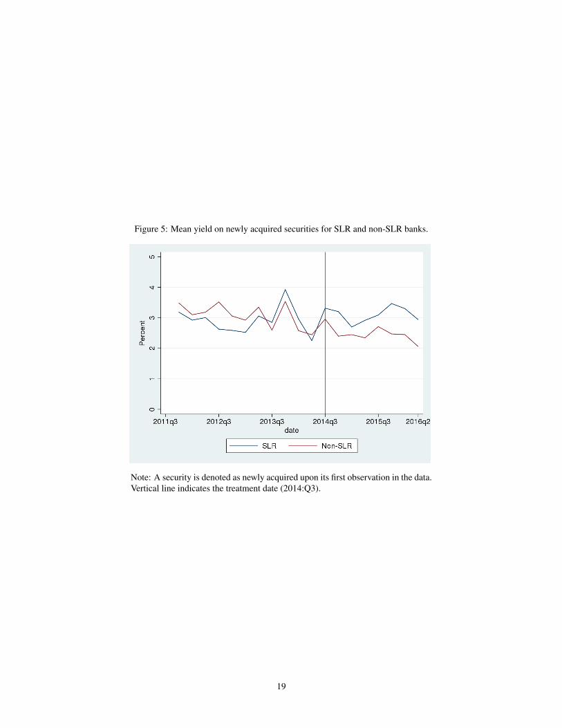
Figure 5: Mean yield on newly acquired securities for SLR and non-SLR banks.

Note: A security is denoted as newly acquired upon its first observation in the data.Vertical line indicates the treatment date (2014:Q3).

19

Figure 6: Mean Leverage Ratio for SLR Tighter, SLR Looser, and non-SLR Banks

Note: Leverage ratio = tier 1 capital divided by total assets for SLR and non-SLR banks.We decompose SLR banks into those who are more or less bound by the SLR. Vertical lineindicates the treatment date (2014:Q3).

20

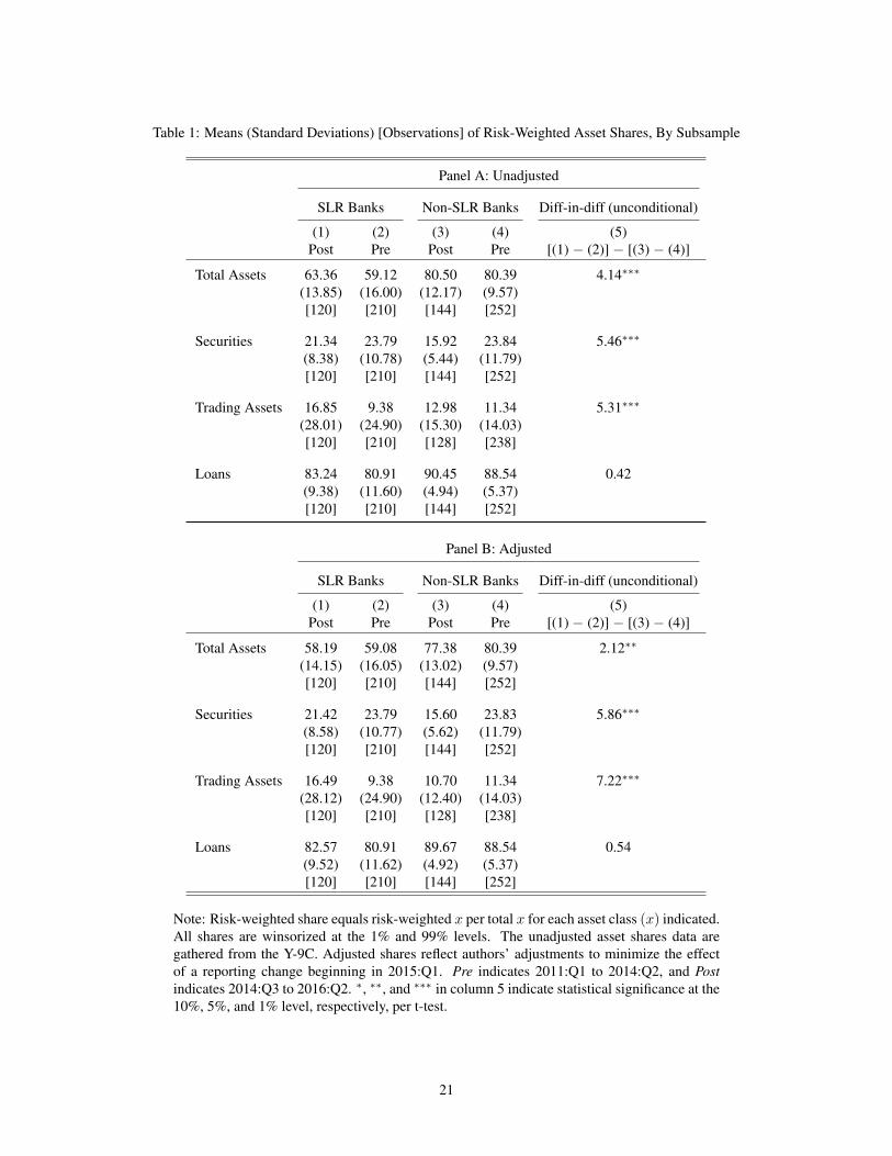
Table 1: Means (Standard Deviations) [Observations] of Risk-Weighted Asset Shares, By Subsample

Panel A: Unadjusted

SLR Banks Non-SLR Banks Diff-in-diff (unconditional)

(1) (2) (3) (4) (5)Post Pre Post Pre [(1) − (2)] − [(3) − (4)]

Total Assets 63.36 59.12 80.50 80.39 4.14∗∗∗

(13.85) (16.00) (12.17) (9.57)[120] [210] [144] [252]

Securities 21.34 23.79 15.92 23.84 5.46∗∗∗

(8.38) (10.78) (5.44) (11.79)[120] [210] [144] [252]

Trading Assets 16.85 9.38 12.98 11.34 5.31∗∗∗

(28.01) (24.90) (15.30) (14.03)[120] [210] [128] [238]

Loans 83.24 80.91 90.45 88.54 0.42(9.38) (11.60) (4.94) (5.37)[120] [210] [144] [252]

Panel B: Adjusted

SLR Banks Non-SLR Banks Diff-in-diff (unconditional)

(1) (2) (3) (4) (5)Post Pre Post Pre [(1) − (2)] − [(3) − (4)]

Total Assets 58.19 59.08 77.38 80.39 2.12∗∗

(14.15) (16.05) (13.02) (9.57)[120] [210] [144] [252]

Securities 21.42 23.79 15.60 23.83 5.86∗∗∗

(8.58) (10.77) (5.62) (11.79)[120] [210] [144] [252]

Trading Assets 16.49 9.38 10.70 11.34 7.22∗∗∗

(28.12) (24.90) (12.40) (14.03)[120] [210] [128] [238]

Loans 82.57 80.91 89.67 88.54 0.54(9.52) (11.62) (4.92) (5.37)[120] [210] [144] [252]

Note: Risk-weighted share equals risk-weighted x per total x for each asset class (x) indicated.All shares are winsorized at the 1% and 99% levels. The unadjusted asset shares data aregathered from the Y-9C. Adjusted shares reflect authors’ adjustments to minimize the effectof a reporting change beginning in 2015:Q1. Pre indicates 2011:Q1 to 2014:Q2, and Postindicates 2014:Q3 to 2016:Q2. ∗, ∗∗, and ∗∗∗ in column 5 indicate statistical significance at the10%, 5%, and 1% level, respectively, per t-test.

21

Table 2: Difference-in-Differences in Risk-weighted Asset Shares

Panel A: Unadjusted

(1) (2) (3) (4)Total Assets Securities Trading Assets Loans

SLR Bank × Post 3.64∗∗ 5.45∗∗ 5.56 0.37(1.43) (2.59) (4.47) (1.72)

Observations 684 684 634 684R-Squared 0.97 0.66 0.78 0.91

Panel B: Adjusted

(1) (2) (3) (4)Total Assets Securities Trading Assets Loans

SLR Bank × Post 1.92 5.88∗∗ 7.51∗ 0.46(3.12) (2.63) (4.18) (1.64)

Observations 684 684 634 684R-Squared 0.83 0.67 0.80 0.92

Note: Reported are OLS estimates of δ from model (1) using panel data on allbanks with at least $50 billion in assets over 2011:Q1 to 2016:Q2. Robust, clus-tered (by bank) standard errors are in parenthesis. Post indicates post-SLR treat-ment (2014:Q3); SLR indicates treated banks (firms with at least $250 billion inassets or over $10 billion in foreign exposures). The regression model includes therisk-based capital ratio and a proxy for the liquidity coverage rule exposure (bothlagged one quarter) and fixed effects (bank and year-quarter). The unadjusted assetshares data are gathered from the Y-9C. Adjusted shares reflect authors’ adjust-ments to minimize the effect of a reporting change beginning in 2015:Q1. Alldependent variables are winsorized at the 1% and 99% levels.∗, ∗∗, and ∗∗∗ denotestatistical significance at the 10%, 5%, and 1% level, respectively.

22

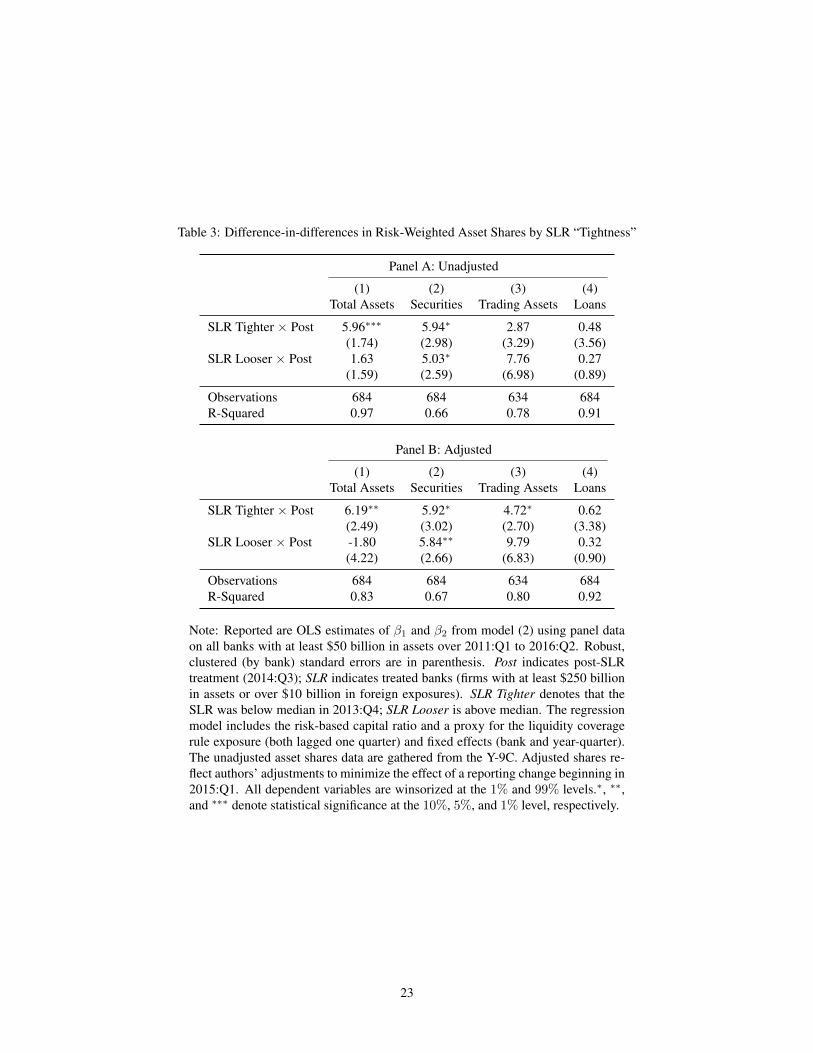
Table 3: Difference-in-differences in Risk-Weighted Asset Shares by SLR “Tightness”

Panel A: Unadjusted

(1) (2) (3) (4)Total Assets Securities Trading Assets Loans

SLR Tighter × Post 5.96∗∗∗ 5.94∗ 2.87 0.48(1.74) (2.98) (3.29) (3.56)

SLR Looser × Post 1.63 5.03∗ 7.76 0.27(1.59) (2.59) (6.98) (0.89)

Observations 684 684 634 684R-Squared 0.97 0.66 0.78 0.91

Panel B: Adjusted

(1) (2) (3) (4)Total Assets Securities Trading Assets Loans

SLR Tighter × Post 6.19∗∗ 5.92∗ 4.72∗ 0.62(2.49) (3.02) (2.70) (3.38)

SLR Looser × Post -1.80 5.84∗∗ 9.79 0.32(4.22) (2.66) (6.83) (0.90)

Observations 684 684 634 684R-Squared 0.83 0.67 0.80 0.92

Note: Reported are OLS estimates of β1 and β2 from model (2) using panel dataon all banks with at least $50 billion in assets over 2011:Q1 to 2016:Q2. Robust,clustered (by bank) standard errors are in parenthesis. Post indicates post-SLRtreatment (2014:Q3); SLR indicates treated banks (firms with at least $250 billionin assets or over $10 billion in foreign exposures). SLR Tighter denotes that theSLR was below median in 2013:Q4; SLR Looser is above median. The regressionmodel includes the risk-based capital ratio and a proxy for the liquidity coveragerule exposure (both lagged one quarter) and fixed effects (bank and year-quarter).The unadjusted asset shares data are gathered from the Y-9C. Adjusted shares re-flect authors’ adjustments to minimize the effect of a reporting change beginning in2015:Q1. All dependent variables are winsorized at the 1% and 99% levels.∗, ∗∗,and ∗∗∗ denote statistical significance at the 10%, 5%, and 1% level, respectively.

23

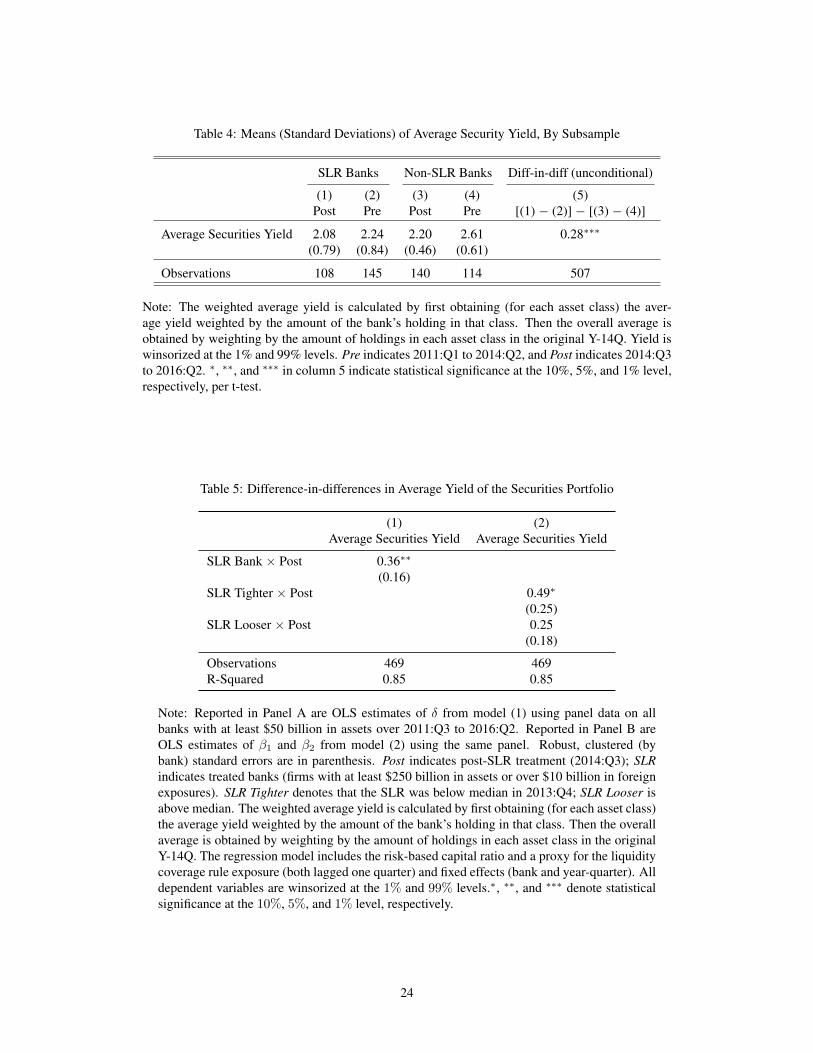
Table 4: Means (Standard Deviations) of Average Security Yield, By Subsample

SLR Banks Non-SLR Banks Diff-in-diff (unconditional)

(1) (2) (3) (4) (5)Post Pre Post Pre [(1) − (2)] − [(3) − (4)]

Average Securities Yield 2.08 2.24 2.20 2.61 0.28∗∗∗

(0.79) (0.84) (0.46) (0.61)

Observations 108 145 140 114 507

Note: The weighted average yield is calculated by first obtaining (for each asset class) the aver-age yield weighted by the amount of the bank’s holding in that class. Then the overall average isobtained by weighting by the amount of holdings in each asset class in the original Y-14Q. Yield iswinsorized at the 1% and 99% levels. Pre indicates 2011:Q1 to 2014:Q2, and Post indicates 2014:Q3to 2016:Q2. ∗, ∗∗, and ∗∗∗ in column 5 indicate statistical significance at the 10%, 5%, and 1% level,respectively, per t-test.

Table 5: Difference-in-differences in Average Yield of the Securities Portfolio

(1) (2)Average Securities Yield Average Securities Yield

SLR Bank × Post 0.36∗∗

(0.16)SLR Tighter × Post 0.49∗

(0.25)SLR Looser × Post 0.25

(0.18)

Observations 469 469R-Squared 0.85 0.85

Note: Reported in Panel A are OLS estimates of δ from model (1) using panel data on allbanks with at least $50 billion in assets over 2011:Q3 to 2016:Q2. Reported in Panel B areOLS estimates of β1 and β2 from model (2) using the same panel. Robust, clustered (bybank) standard errors are in parenthesis. Post indicates post-SLR treatment (2014:Q3); SLRindicates treated banks (firms with at least $250 billion in assets or over $10 billion in foreignexposures). SLR Tighter denotes that the SLR was below median in 2013:Q4; SLR Looser isabove median. The weighted average yield is calculated by first obtaining (for each asset class)the average yield weighted by the amount of the bank’s holding in that class. Then the overallaverage is obtained by weighting by the amount of holdings in each asset class in the originalY-14Q. The regression model includes the risk-based capital ratio and a proxy for the liquiditycoverage rule exposure (both lagged one quarter) and fixed effects (bank and year-quarter). Alldependent variables are winsorized at the 1% and 99% levels.∗, ∗∗, and ∗∗∗ denote statisticalsignificance at the 10%, 5%, and 1% level, respectively.

24

Table 6: Extensive Margin, Purchased Securities

Panel A: Difference-in-differences in Yield

(1) (2) (3) (4)All Banks, WLS All Banks, OLS Non-Custody Banks, WLS Non-Custody Banks, OLS

Post × SLR Bank 0.38∗∗ 0.39 0.50∗∗ 0.62∗∗

(0.18) (0.27) (0.19) (0.24)

Observations 312620 313004 269510 269868R-Squared 0.20 0.14 0.20 0.13

Panel B: Difference-in-differences in Yield, By SLR “Tightness”

(1) (2) (3) (4)All Banks, WLS All Banks, OLS Non-Custody Banks, WLS Non-Custody Banks, OLS

SLR Tighter × Post 0.33 0.47 0.61 1.01∗∗

(0.28) (0.38) (0.37) (0.38)SLR Looser × Post 0.42∗∗ 0.28 0.44∗∗ 0.28

(0.17) (0.21) (0.17) (0.19)

Observations 312620 313004 269510 269868R-Squared 0.20 0.14 0.20 0.14

Note: Reported are OLS estimates of of δ from model (3) using panel data on all banks with at least $50 billion inassets over 2011:Q3 to 2016:Q2. Robust, clustered (by bank) standard errors are in parenthesis. Post indicates post-SLR treatment (2014:Q3); SLR indicates treated banks (firms with at least $250 billion in assets or over $10 billion inforeign exposures). SLR Tighter denotes that the SLR was below median in 2013:Q4; SLR Looser is above median.The regression model includes the risk-based capital ratio and a proxy for the liquidity coverage rule exposure (bothlagged one quarter) and fixed effects (bank and year-quarter). All dependent variables are winsorized at the 1% and99% levels.∗, ∗∗, and ∗∗∗ denote statistical significance at the 10%, 5%, and 1% level, respectively.

25

Table 7: Means (Standard Deviations) [Observations] of Overall Risk Measures, By Subsample

SLR Banks Non-SLR Banks Diff-in-diff (unconditional)

(1) (2) (3) (4) (5)Post Pre Post Pre [(1) − (2)] − [(3) − (4)]

ROA 1.02 0.95 0.82 0.83 0.07∗

(0.79) (0.79) (0.56) (0.76)[120] [210] [144] [252]

ROA Volatility 0.20 0.28 0.27 0.55 0.20∗∗∗

(0.16) (0.21) (0.61) (0.89)[120] [210] [144] [252]

Z Score 139.76 94.90 160.53 92.11 -23.55∗∗∗

(55.94) (40.94) (53.42) (30.28)[120] [210] [144] [252]

Equity volatility 1.49 1.68 1.62 1.65 -0.17∗∗∗

(0.16) (0.34) (0.15) (0.31)[104] [182] [96] [154]

5-year CDS spread 0.71 1.22 1.11 1.83 0.12∗∗∗

(0.18) (0.47) (0.57) (0.84)[104] [196] [88] [154]

Implied vol. 38.54 45.87 38.08 45.47 -0.60(2.54) (4.00) (3.22) (7.59)[104] [182] [96] [154]

Put option Delta -0.02 -0.07 -0.02 -0.07 -0.00(0.01) (0.01) (0.01) (0.02)[104] [182] [96] [154]

Note: ROA volatility is calculated as the rolling 4-quarter standard deviation, excluding periodswhere treatment and control dates overlap. Equity volatility is calculated as the quarterly standarddeviation of the log difference in daily stock price for public firms. Implied volatilites are on a50% out-of-the-money option that expires in 1 year. Implied deltas are calculated using the Black-Scholes formula. All risk measures are winsorized at the 1% and 99% levels. Pre indicates 2011:Q1to 2014:Q2, and Post indicates 2014:Q3 to 2016:Q2. ∗, ∗∗, and ∗∗∗ in column 5 indicate statisticalsignificance at the 10%, 5%, and 1% level, respectively, per t-test.

26

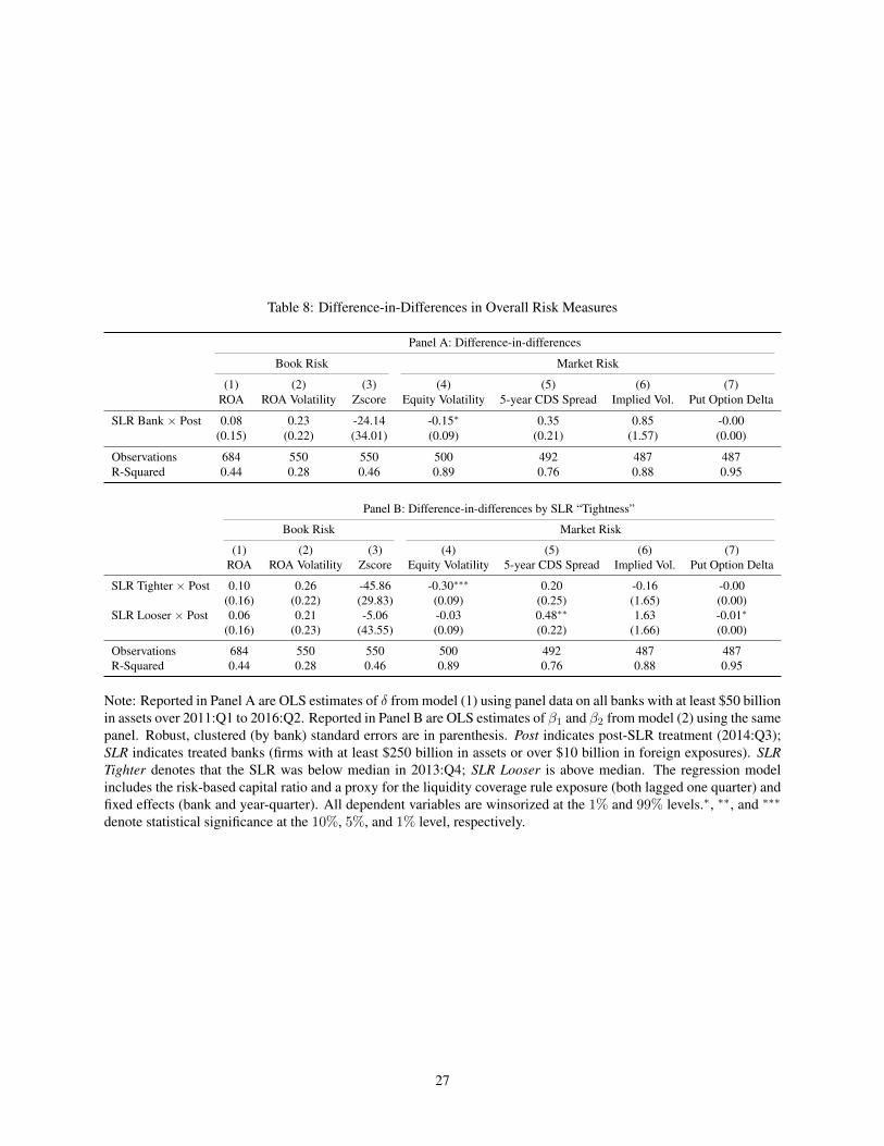
Table 8: Difference-in-Differences in Overall Risk Measures

Panel A: Difference-in-differences

Book Risk Market Risk

(1) (2) (3) (4) (5) (6) (7)ROA ROA Volatility Zscore Equity Volatility 5-year CDS Spread Implied Vol. Put Option Delta

SLR Bank × Post 0.08 0.23 -24.14 -0.15∗ 0.35 0.85 -0.00(0.15) (0.22) (34.01) (0.09) (0.21) (1.57) (0.00)

Observations 684 550 550 500 492 487 487R-Squared 0.44 0.28 0.46 0.89 0.76 0.88 0.95

Panel B: Difference-in-differences by SLR “Tightness”

Book Risk Market Risk

(1) (2) (3) (4) (5) (6) (7)ROA ROA Volatility Zscore Equity Volatility 5-year CDS Spread Implied Vol. Put Option Delta

SLR Tighter × Post 0.10 0.26 -45.86 -0.30∗∗∗ 0.20 -0.16 -0.00(0.16) (0.22) (29.83) (0.09) (0.25) (1.65) (0.00)

SLR Looser × Post 0.06 0.21 -5.06 -0.03 0.48∗∗ 1.63 -0.01∗

(0.16) (0.23) (43.55) (0.09) (0.22) (1.66) (0.00)

Observations 684 550 550 500 492 487 487R-Squared 0.44 0.28 0.46 0.89 0.76 0.88 0.95

Note: Reported in Panel A are OLS estimates of δ from model (1) using panel data on all banks with at least $50 billionin assets over 2011:Q1 to 2016:Q2. Reported in Panel B are OLS estimates of β1 and β2 from model (2) using the samepanel. Robust, clustered (by bank) standard errors are in parenthesis. Post indicates post-SLR treatment (2014:Q3);SLR indicates treated banks (firms with at least $250 billion in assets or over $10 billion in foreign exposures). SLRTighter denotes that the SLR was below median in 2013:Q4; SLR Looser is above median. The regression modelincludes the risk-based capital ratio and a proxy for the liquidity coverage rule exposure (both lagged one quarter) andfixed effects (bank and year-quarter). All dependent variables are winsorized at the 1% and 99% levels.∗, ∗∗, and ∗∗∗

denote statistical significance at the 10%, 5%, and 1% level, respectively.

27

28

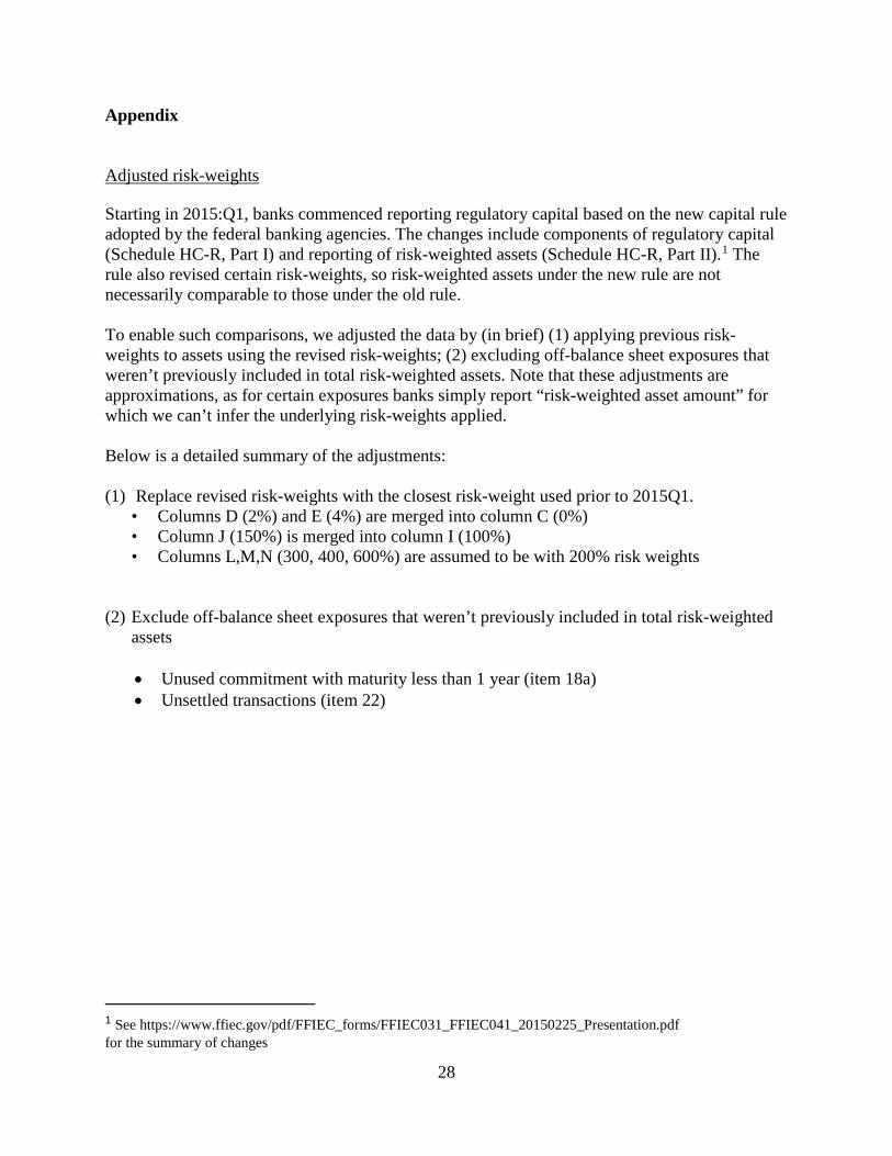
Appendix Adjusted risk-weights Starting in 2015:Q1, banks commenced reporting regulatory capital based on the new capital rule adopted by the federal banking agencies. The changes include components of regulatory capital (Schedule HC-R, Part I) and reporting of risk-weighted assets (Schedule HC-R, Part II).1 The rule also revised certain risk-weights, so risk-weighted assets under the new rule are not necessarily comparable to those under the old rule. To enable such comparisons, we adjusted the data by (in brief) (1) applying previous risk-weights to assets using the revised risk-weights; (2) excluding off-balance sheet exposures that weren’t previously included in total risk-weighted assets. Note that these adjustments are approximations, as for certain exposures banks simply report “risk-weighted asset amount” for which we can’t infer the underlying risk-weights applied. Below is a detailed summary of the adjustments: (1) Replace revised risk-weights with the closest risk-weight used prior to 2015Q1.

• Columns D (2%) and E (4%) are merged into column C (0%) • Column J (150%) is merged into column I (100%) • Columns L,M,N (300, 400, 600%) are assumed to be with 200% risk weights

(2) Exclude off-balance sheet exposures that weren’t previously included in total risk-weighted

assets

• Unused commitment with maturity less than 1 year (item 18a) • Unsettled transactions (item 22)

1 See https://www.ffiec.gov/pdf/FFIEC_forms/FFIEC031_FFIEC041_20150225_Presentation.pdf for the summary of changes

29

Constructing Average Securities Yield Calculating the weighted average yield by combining all asset types may skew the average yield due to differences in asset class composition between our matched sample and the full Y-14 data. To mitigate this concern, we construct the weighted average yield in a two-step process. First, for each bank-quarter, within each asset class we calculate the value-weighted average yield, i.e. weighted by the market value of each security in the class. We then weight the weighted average yield for each class by the value share the asset class represents within the bank-quarter in the overall Y-14 data.

For example, suppose a bank’s securities portfolio in a given quarter, as reported in the Y-14, is composed of 10% corporate bonds and 90% Treasuries by value. Suppose the value-weighted average yield of corporate bonds in our sample is 4% and that of Treasuries is 2%. Then our final yield would be:

(0.1 × 4%) + (0.9 × 2%) = 2.2%.

The following notation formalizes this calculation. For each security s belonging to asset class c held by bank i in quarter t, we first calculate the average yield of the asset class c held by the bank:

� 𝑟𝑟𝑖𝑖𝑖𝑖𝑖𝑖𝑖𝑖 × 𝑣𝑣𝑖𝑖𝑖𝑖𝑖𝑖𝑖𝑖𝑖𝑖 in class 𝑖𝑖

= 𝑤𝑤𝑖𝑖𝑖𝑖𝑖𝑖

where r is the security’s yield and v is the ratio of the security’s market value to the total

market value of all securities in asset class c held by bank i. Thus, 𝑤𝑤𝑖𝑖𝑖𝑖𝑖𝑖 is the value-weighted average yield for each asset class c. Then, we calculate the average across the asset classes:

�𝑤𝑤𝑖𝑖𝑖𝑖𝑖𝑖 × 𝑘𝑘𝑖𝑖𝑖𝑖𝑖𝑖𝑖𝑖

= 𝑦𝑦𝑖𝑖𝑖𝑖

where k is the share of the bank’s portfolio belonging to class c as reported in the Y-14.

Thus, yit is our final bank-quarter average securities yield observation.