Leverage and the Beta Anomaly1

Malcolm Baker

Harvard Business School and NBER

mbaker@hbs.edu

617-495-6566

Mathias F. Hoeyer

University of Oxford

mfhoeyer@gmail.com

Jeffrey Wurgler (corresponding author)

NYU Stern School of Business and NBER

jwurgler@stern.nyu.edu

212-998-0367

January 14, 2019

Abstract

The well-known weak empirical relationship between beta risk and the cost of equity--the

beta anomaly--generates a simple tradeoff theory: As firms lever up, the overall cost of

capital falls as leverage increases equity beta, but as debt becomes riskier the marginal

benefit of increasing equity beta declines. As a simple theoretical framework predicts, we

find that leverage is inversely related to asset beta, including upside asset beta, which is

hard to explain by the traditional leverage tradeoff with financial distress that emphasizes

downside risk. The results are robust to a variety of specification choices and control

variables.

1 For helpful comments we thank Hui Chen, Robin Greenwood, Sam Hanson, Lasse Pedersen, Thomas

Philippon, Ivo Welch, and seminar participants at the American Finance Association, Capital Group,

George Mason University, Georgetown University, the Ohio State University, NYU, the New York Fed,

Southern Methodist University, University of Amsterdam, University of Cambridge, University of Tokyo,

University of Toronto, University of Miami, University of Utah, USC, and University of Warwick. Baker

and Wurgler also serve as consultants to Acadian Asset Management. Baker gratefully acknowledges

financial support from the Division of Research of the Harvard Business School.

1

Leverage and the Beta Anomaly

Abstract

The well-known weak empirical relationship between beta risk and the cost of equity--the beta anomaly--generates a simple tradeoff theory: As firms lever up, the overall cost of capital falls as leverage increases equity beta, but as debt becomes riskier the marginal benefit of increasing equity beta declines. As a simple theoretical framework predicts, we find that leverage is inversely related to asset beta, including upside asset beta, which is hard to explain by the traditional leverage tradeoff with financial distress that emphasizes downside risk. The results are robust to a variety of specification choices and control variables.

2

Literally millions of students have been taught corporate finance under the assumption of

the Capital Asset Pricing Model (CAPM) and integrated equity and debt markets. Yet, it is well

known that the link between textbook measures of risk and realized returns in the stock market is

weak, or even backward. For example, a dollar invested in a low beta portfolio of U.S. stocks in

1968 grows to $70.50 by 2011, while a dollar in a high beta portfolio grows to just $7.61.1 The

evidence on the anomalously low returns to high-beta stocks begins as early as Black, Jensen,

and Scholes (1972). In a recent contribution, Bali, Brown, Murray, and Tang (2017) identify it as

“one of the most persistent and widely studied anomalies in empirical research of security

returns” (p. 2369). A large literature has come to view the beta anomaly, and related anomalies

based on total or idiosyncratic risk, as evidence of mispricing as opposed to a misspecified risk

model. In this paper, we consider these explanations sufficiently plausible to consider their

implications for leverage. In doing so, we bring ideas from the anomalies literature into corporate

finance, which often assumes efficient and integrated securities markets to highlight other

frictions.

We show that a beta anomaly in equity markets—absent any other deviations from the

Modigliani-Miller setup—leads to a simple tradeoff. Intuitively, under the anomaly, beta risk is

overvalued in equity securities, but not in debt securities. Ideally, then, to minimize the cost of

capital, risk is concentrated in equity. A firm will always want to issue as much riskless debt as it

can. This lowers the cost of equity by increasing its beta without any “inefficient” transfer of risk

from equity to debt. But, as debt becomes risky, further increases in leverage have a cost.

Shifting overvalued risk in equity securities to fairly valued risk in debt securities increases the

                                                                                                                         1 See Baker, Bradley, and Taliaferro (2014).

3

overall cost of capital. For firms with high-beta assets, this increase is high even at low levels of

leverage. For firms with low-beta assets, this increase remains low until leverage is high. Using

the Merton (1974) model to characterize the functional form of debt betas and the underlying

transfer of risk from equity to debt, we show that there is an interior optimum leverage ratio that

is inversely related to asset beta.

The theory’s immediate prediction is that leverage is negatively related to asset beta.

Empirically, we confirm that there is indeed a robust negative relationship between leverage and

asset beta. The relationship remains strong when controlling for overall asset variance (a control

for distress risk), using alternative measures of leverage and industry measures of asset beta and

overall risk, and including various other control variables.

While it is reassuring that the beta anomaly tradeoff generates a leverage-asset beta

prediction that is borne out in the data, an obvious alternative explanation is based on the

standard tradeoff theory, which also predicts an inverse relationship between leverage and risk

(most intuitively, total asset risk, not asset beta). For example, Long and Malitz (1985) include

systematic asset risk, not just overall risk, in leverage regressions with the traditional tradeoff

between taxes and financial distress costs in mind. We do not wish to cast doubt on the relevance

of the standard tradeoff theory. Instead, we derive and test additional predictions of the beta

anomaly tradeoff to show that it has incremental explanatory power.

In particular, we prove that, under a beta anomaly, both “upside” and “downside” betas

are inversely related to leverage. Financial distress costs, on the other hand, clearly emphasize

downside risk. And, consistent with the beta anomaly tradeoff, we find that leverage is indeed

inversely related to upside asset beta as well. In some specifications, the upside beta relationship

is actually stronger than the downside beta relationship. While our results do not rule out the

4

traditional tradeoff theory, given that downside beta still matters, this prediction and empirical

relationship is most easily explained by a beta anomaly tradeoff.

We tentatively suggest that the beta anomaly tradeoff may also help to explain extremely

high and low leverage levels that challenge the standard tradeoff. For instance, Graham (2000)

and others have pointed out that hundreds of profitable firms, with high marginal tax rates,

maintain essentially zero leverage. This is often called the low-leverage puzzle. Conversely, a

number of other profitable firms maintain high leverage despite no tax benefit. The beta anomaly

tradeoff could help to explain these patterns. If low leverage firms have determined that the tax

benefit of debt is less than the opportunity cost of transferring risk to lower-cost equity, low

leverage may be optimal even in the presence of additional frictions; a minor, realistic

transaction cost of issuance could drive some firms to zero leverage. Meanwhile, low asset beta

firms with no tax benefits of debt still resist equity because of its high risk-adjusted cost at low

levels of leverage, and instead use a very large fraction of debt finance.

In addition to providing a novel theory of leverage based on a single deviation from the

Modigliani-Miller setup, the beta anomaly approach has an attractive and unifying conceptual

feature. The traditional tradeoff theory, under rational asset pricing, cannot fit both the

leverage and asset pricing evidence on the pricing of beta. If beta is truly a measure of risk

relevant for capital structure, then presumably it would also help to explain the cross section of

asset returns, which it does not. Investors, recognizing the associated investment opportunities,

would demand higher returns on assets exposed to the systematic risk of fire sales, with high

risk-adjusted costs of financial distress. If beta is not a measure of risk, as the large literature that

follows Fama and French (1992, 1993) has claimed, then asset beta should not be a constraint on

leverage, after controlling for total asset risk. Although the beta anomaly is far from the only

5

force at work in real-life capital markets—following the standard approach in corporate finance

theory, we focus on a single “friction” (the beta anomaly) for simplicity—it is worth noting that

it offers an internally consistent explanation for both of these patterns.

Section 1 briefly reviews the beta anomaly and derives optimal leverage under the

anomaly. Sectional 2 contains empirical hypotheses and tests. Section 3 concludes.

1. The Beta Anomaly Tradeoff

1.1. Motivation and Setup

Over the long run, riskier asset classes have earned higher returns, but the historical risk-

return tradeoff within the stock market is flat at best. The Capital Asset Pricing Model (CAPM)

predicts that the expected return on a security is proportional to its beta, but in fact stocks with

higher beta have tended to earn lower returns, particularly on a risk-adjusted basis. As mentioned

earlier, Bali, Brown, Murray, and Tang (2017) highlight the beta anomaly as one of the most

prominent of the many dozen anomalies studied in the literature. We refer the reader to that

paper, as well as Baker, Bradley, and Wurgler (2011) or Hong and Sraer (2016) for an overview

of the large literature that shows the beta anomaly’s robustness across sample periods and

international markets and reviews some of its theoretical foundations.

The simple linear specification for the beta anomaly that we employ here is

, (1)

where rf is the risk free rate, rp is the market risk premium, and γ < 0 measures the size of the

anomaly. The beta anomaly is that a stock has “alpha” and the alpha falls with its beta.

A few comments on this simple functional form. In terms of the “neutral point” where

equity risk is fairly priced, Eq. (1) assumes this takes place at an equity beta of 1.0. The equity

( ) pefee rrr βγβ ++−= 1

6

premium puzzle suggests that, historically, that location might be at a higher level. But, even if

equity were undervalued or overvalued on average, the mean leverage behavior would change,

but predictions about the cross-section of leverage, our focus here, would not.

If the beta anomaly extended in equal force into debt, Modigliani-Miller irrelevance

would still hold. Neither the literature nor our own tests indicate a meaningful beta anomaly in

debt, however. In Frazzini and Pedersen (2014), short-maturity corporate bonds of low risk firms

have marginally higher bond-market-beta risk-adjusted returns, but bond index betas have little

relationship to stock index betas, the basis of the beta anomaly. In fact, Fama and French (1993)

show that stock market betas are nearly identical for bond portfolios of various ratings, and

Baele, Bekaert, and Inghelbrecht (2009) find that even the sign of the correlation/beta between

government bond and stock indexes is unstable.2

With a beta anomaly in equity, the overall cost of capital depends not only on asset beta

but on leverage:

, (2)

where  is asset beta and e is capital structure as measured by the ratio of equity to firm value.

The second to last term—the asset beta minus one times γ —is the uncontrollable reduction in

the cost of capital that comes from having high-risk assets. The last term is the controllable cost

of having too little leverage while debt beta remains low.

An advantage of using the CAPM to develop comparative statics is to see the familiar

textbook transfers of beta risk from equity to debt as leverage increases. However, any asset

                                                                                                                         2 Nonetheless, just to be sure, we directly compared the returns on beta-sorted stock portfolios with beta-risk-adjusted corporate bond portfolios and can easily reject an integrated beta anomaly. These results are omitted for brevity but available on request. See Harford, Martos-Vila, and Rhodes-Kropf (2015) for perspectives on financing under (non-beta-based) debt mispricing.

( ) ( ) ( ) ( )( )γβγββ 1111 −−−−++=−+= dapafde errreereWACC

βa

7

pricing model that features a stronger beta anomaly in equity will lead to the same qualitative

conclusions.

1.2. Optimal Capital Structure

Next we outline a simple, static model of optimal capital structure with no frictions other

than a beta anomaly. There are no taxes, transaction costs, issuance costs, incentive or

information effects of leverage, or costs of financial distress. It is interesting that unlike other

tradeoff approaches, which require one friction to limit leverage on the low side and another to

limit it on the high side, this single mechanism can drive an interior optimum.

The optimal capital structure minimizes the last term of (2) by satisfying the first order

condition for e. With the further assumption of a differentiable debt beta, for a given level of

asset beta the optimal capital ratio e* satisfies

(3)

or, in terms of optimal debt beta,

.

The optimum leverage does not depend on the size of the beta anomaly, but this is a bit of a

technicality. If there were any other frictions associated with leverage, such as taxes or financial

distress costs, the anomaly’s size would become relevant.

1.2.1. Observation 1: Firms will issue some debt, and as much debt as possible as long as it

remains risk-free

The first order condition cannot be satisfied as long as the debt beta is zero. At a zero

debt beta, the left side of Equation (3) is positive (recall γ < 0). In other words, issuing more

−γ 1−βd e*(βa ),βa⎡⎣ ⎤⎦+ 1− e

*(βa )⎡⎣ ⎤⎦∂βd e

*(βa ),βa⎡⎣ ⎤⎦∂e

⎧⎨⎪

⎩⎪

⎫⎬⎪

⎭⎪= 0

β*d e*(βa ),βa⎡⎣ ⎤⎦=1+ 1− e

*(βa )⎡⎣ ⎤⎦∂βd e

*(βa ),βa⎡⎣ ⎤⎦∂e

8

equity at the margin will raise the cost of capital. With zero debt, the asset beta is equal to the

equity beta and the WACC reduces to:

WACC(1) = (βa −1)γ + rf +βarp . (4)

A first-order Taylor approximation around shows that even marginal debt will decrease the

cost of capital:

. (5)

At first blush, this would seem to deepen the low leverage puzzle of Graham (2000). One

might ask why nonfinancial firms do not increase their leverage ratios further to take advantage

of the beta anomaly: It is initially unclear how the low leverage ratios of nonfinancial firms

represent an optimal tradeoff between the tax benefits of interest and the costs of financial

distress, much less an extra benefit of debt arising from the mispricing of low risk stocks.

The answer from Equation (3) is that many low leverage firms—for example, the

stereotypical unprofitable technology firm—already start with a high asset beta or overall asset

risk. Their assets are already quite risky at zero debt. Even at modest levels of debt, meaningful

risk starts to be transferred to debt. While Equation (3) cannot on its own explain why a firm

would have exactly zero debt, it can explain why some firms have low levels of debt, despite the

tax benefits and modest costs of financial distress.

1.2.2 Observation 2: Leverage has an interior optimum

Zero equity is also not optimal. With all debt finance, the debt beta equals the asset beta

and Equation (2) reduces to the traditional WACC formula without the beta anomaly. This

establishes that optimum leverage must be interior. The intuition is that, with the assumption of

fairly priced debt, the firm will be fairly priced if it is funded entirely with debt, i.e. 100%

leveraged. Can it increase value by reducing its leverage ratio? Yes. This new equity, an out-of-

e =1

WACC(e) ≈WACC(1)+ (1− e)λ <WACC(1)

9

the-money call option, will be high risk, and hence overvalued. As a consequence, neither 0%

nor 100% leverage are optimal, so there must be an interior optimum.

To further our understanding of optimal debt levels, we must characterize the dynamics

underlying transfer of risk from equity to debt with increasing levels of leverage, and in

particular the dependence of debt beta on leverage. A natural candidate for the functional form of

debt betas is the Merton (1974) model. Merton uses the isomorphic relationship between levered

equity, a European call option, and the accounting identity to derive the value of a

single, homogenous debt claim, such that

, (6)

where V is firm value with volatility σ, D is the value of the debt with maturity in and face

value B. Let be the firm variance over time, and the debt ratio, where debt is

valued at the risk free rate, thus d is an upward biased estimate of the actual market based debt

ratio (Merton, pp. 454-455). Here, is the cumulative standard normal distribution and x1

and x2 are the familiar terms from the Black-Scholes formula.

Following the approach of Black and Scholes (1973), we arrive at the debt beta:

. (7)

Here DV is the first derivative of the debt value given in Equation (6) with respect to V. In the

Merton model, debt is equivalent to a riskless debt claim less a put option. It follows that the

derivative DV is equivalent to the negative of the derivative of the value of this put option. That

is, the derivative (or delta) of the put option on the underlying firm value is ,

thus . Substituting for Equation (2), the debt beta can be written as

D =V −E

D(d,T ) = Be−rfτΦ x2 (d,T )[ ]+V 1−Φ x1(d,T )[ ]{ }

τ

T =σ 2τ d ≡ Be−rfτ

V

Φ(x)

βd = βaVDDV

Δ put = − 1−Φ(x1)[ ]

Dv ≡ −Δ put =1−Φ(x1)

10

( ) ad dX ββ = , (8)

where )(1)()(1

12

1)( xxdxdX Φ−+Φ

Φ−= is positive. Further, we have that the debt beta is bounded:

( ){ } 0lim 0 ==→ add dX ββ , and ( ){ } aadd dX βββ ==∞→lim ,

in line with the boundary conditions of the debt and in support of the limiting conditions

necessary to establish the claim of an interior optimum leverage.

The factor is equivalent to the delta of an equity claim with spot price equal to V

and exercise price equal to face value of the debt B. In light thereof, the debt beta can be seen to

be driven by the increasing value loss in default. If then the debt beta will be continuous

and strictly increasing in d. Now rewriting Equation (8),

, (9)

and following the limits above it can be seen that . Consequently, in

Equation (9) can be interpreted as the conditional expectation of firm value given it is larger than

the face value of debt, times the probability of the firm value being larger than the face value of

debt. This is effectively the amount of firm risk carried by the debt.

On closer inspection, the debt beta in Equation (8) can be written, showing its full

functional dependence, . In our framework, however, the measure of leverage is not

d, but rather the market-based capital ratio, e, that is given by

, (10)

and is continuous and strictly decreasing in d.

Φ(x1)

βa > 0

βd = βaV −VΦ(x1)

D

0 ≤V −VΦ(x1) ≤ D VΦ(x1)

βd (d,βa,T )

e(d,T ) = V −DV

=Φ(x1)− dΦ(x2 )

11

By expressing the debt beta in Equation (8) parametrically as a function of the equity

ratio in Equation (10) with d as a shared parameter, holding all else equal, the derivative of the

debt beta in Equation (3) is equivalent to:

, and ∂βd (d,βa,T ) /∂d∂e(d, t) /∂d

= −M d( )βa . (11)

The intuition of M(d) is not important. Its first feature of M(d) is that it does not depend on the

asset beta βa itself. So, we can separate out the transfer of risk—which depends on d and the

distribution of firm values characterized by the inputs of total risk, time to maturity, the riskless

rate, and the face value of debt—from the specific risk transferred:

M (d) =Φ(x1)Φ(x2 )+Φ(x2 )

φ (x1 )σ τ

+ 1−Φ(x1)[ ] φ (x2 )σ τ−Φ(x2 )

1−Φ(x1)+ dΦ(x2 )[ ]2 Φ(x2 )− φ (x2 )σ τ

+ φ (x1 )dσ τ

⎡⎣ ⎤⎦. (12)

A second feature of M is that it is positive, so the debt beta falls as the capital ratio increases.

It’s worth mentioning that a cost of equity anomaly in which average returns vary but risk

does not (say, Internet or blockchain assets are overvalued, or more generally the type of

mispricing described in Baker and Wurgler (2002)) does not lead to an interior optimum leverage

on its own. Without another friction and without the issuance itself changing valuations, such as

downward sloping demand, one gets a corner solution of all equity if equity is overvalued or all

debt if equity is undervalued.

Stein (1996) solves this problem by adding costs of financial distress. A mispricing in

which risk varies but average returns do not, such as the beta anomaly, is fundamentally different

because the act of levering or delevering itself changes the risk of the equity, and hence how

much it is mispriced. As just shown, overvalued firms may now want to issue a small amount of

debt, and undervalued firms will not fund themselves with 100% debt because as leverage rises

∂βd (e(d,T ),βa,T )∂e(d,T )

=∂βd (d,βa,T ) /∂d∂e(d,T ) /∂d

12

their equity is no longer undervalued. This mechanism is not present in Stein (1996), and allows

us to derive an interior optimum based on a beta anomaly alone.

1.2.3 Observation 3: The optimal leverage ratio is decreasing in asset beta

This is a basic observation and an intuitive, testable prediction. With the Merton

assumptions, and with no frictions other than a beta anomaly in equity, the optimal level of

capital, e* in Equation (3), can be expressed with Equation (8) and (11) as

e*(d*,βa ) =1−1

M (d*)1−βd (d

*,βa )βa

⎛

⎝⎜

⎞

⎠⎟=1−

1M (d*)

1βa− X(d*)

⎛

⎝⎜

⎞

⎠⎟ . (13)

Holding the positive functions X and M constant—we are varying the asset beta without

changing the overall level of risk—the optimal level of capital is increasing in asset beta:

∂e*(d*,βa )∂βa

=1

M (d*)βa2 ≥ 0 . (14)

We outlined the intuition in the introduction. Under the beta anomaly, beta is overvalued

in equity securities. Ideally, to minimize the cost of capital, risk is concentrated in equity. This

led to the first observation that firms will issue as much risk-free debt as possible. This lowers

the WACC through an increase in the cost of equity due to its increased beta. Once debt becomes

risky, further increases in leverage, or reductions in equity capital e, have a cost. At that point, M

is greater than zero. Shifting overvalued risk in equity to fairly valued risk in debt increases the

cost of capital. For firms with high-beta assets, this increase is high even at low levels of

leverage. For firms with low-beta assets, this increase remains low until leverage is high.

More formally, we can show that:

, , and ∂2βd (e,βa,T )∂βa∂e

< 0 . (15)

The first two partial derivatives of the debt beta with respect to the equity ratio and the asset beta

∂βd (e,βa,T )∂e

< 0 ∂βd (e,βa,T )∂βa

≥ 0

13

follow directly from Equation (9) and the assumption that . Furthermore, since the asset

beta is simply a positive scalar, the cross-partial derivative with the equity ratio must have the

same sign as the partial derivative with respect to the equity ratio.

We can now sign the change in the optimal capital ratio as a function of the underlying

asset beta in the more general case. Taking the derivative of e* with respect to asset beta:

. (16)

The first term is positive using the signs of the partial derivatives in Equation (15). The second

term is the second order condition at the optimal leverage ratio defined in Equation (3). It

follows from Cargo (1965) that the second order condition is positive, if and only if both the debt

beta in Equation (8) and one minus the capital ratio in Equation (10) are strictly increasing in d

and Equation (11) is negative, which we have already established.

1.2.4 Observation 4: Upside and downside asset beta are equally important in determining

optimal leverage.

Although the mechanism is very different, the predictions so far are intuitively consistent

with the standard tradeoff theory and associated evidence. This is encouraging but it is also

important to derive a testable prediction that allows us to empirically distinguish the beta

anomaly tradeoff from the costs of financial distress and the traditional tradeoff. To do this, we

make the simple observation that in the traditional tradeoff, only downside beta, not upside beta,

increases the costs of financial distress and therefore reduces optimal leverage. In contrast, in the

βa > 0

de*(βa )dβa

= − −∂βd e*,βa( )

∂βa+ 1− e*(βa )⎡⎣ ⎤⎦

∂2βd e*,βa( )∂e∂βa

⎡

⎣⎢⎢

⎤

⎦⎥⎥×

−2∂βd e*(βa ),βa( )

∂e+ 1− e*(βa )⎡⎣ ⎤⎦

∂2βd e*(βa ),βa( )∂e2

⎡

⎣⎢⎢

⎤

⎦⎥⎥

−1

14

beta anomaly tradeoff, the effect is symmetric. To show this formally, we repeat the previous

exercise with a version of Equation (1) that separates beta into upside and downside components:

re = β + +β − −1( )γ + rf + β + +β −( )rp , (17)

which we define in the semivariance spirit of Markowitz (1959) and Hogan and Warren (1974).3

We can now substitute this decomposition of the asset beta into (13),

−+ += aaa βββ , (18)

which implies that the optimal capital structure takes the following form:

e*(d*,βa ) =1−1

M (d*)1

βa+ +βa

−− X(d*)

⎛

⎝⎜

⎞

⎠⎟ . (19)

This means that once again holding the positive functions X and M constant, the optimal level of

capital is rising to the same degree in both upside and downside asset beta, as in Equation (14).

Again, there is a straightforward intuition for Equation (19). The character of total risk, as

defined in the functions M and X, is what dictates the transfer of risk from equity to debt.

Holding this transfer of risk constant, the optimal level of capital is increasing in any measure of

mispriced asset risk, whether upside or downside.

1.2.5 Observation 5: A negative empirical relationship between equity beta and leverage is

sufficient to prove a negative empirical relationship between asset beta and leverage

The initial step in our empirical analysis is to confirm a negative relationship between

asset beta and leverage. However, to measure asset beta directly, all liabilities must be traded,

which is rarely the case, so the traditional method of estimating asset beta is simply to assume

                                                                                                                         

3 [ ] −+

==

− +=−−+−−≡ ∑∑ ≤>ββµµµµβ

n

j rmjmijin

j rmjmijim

TjmTjmIrrIrrn

r 1 ,,1 ,,1

,,))(())((

)var(1

.

15

that debt betas are zero. Observation 5 is housekeeping that allows us to avoid having to

condition a negative leverage-asset beta link on a zero debt beta assumption. If leverage rises as

equity beta falls, then asset beta must fall too through a simple Modigliani and Miller logic and

absolute priority of returns. If we find that the equity beta is lower and leverage is higher, then

the asset beta must be lower. Thus, a negative relationship between equity beta and leverage

further implies a negative relationship between asset beta and leverage.

1.2.6. Further Remarks

Like all theoretical work on leverage, our framework clearly makes tradeoffs between

tractability and realism. But, one broader question concerns what do managers really need to

know, in practice, in order to drive the predictions made above? In the model, managers must

understand how their leverage choice affects their cost of capital at the margin. In “reality,” a

reasonable suggestion is that managers estimate their cost of equity capital in the process of

estimating the fundamental value of their common stock. The manager’s valuation depends, as in

textbooks, on his or her best guess of future cash flows and the firm’s true, rational cost of

capital.

In such calculations, according to surveys by Graham and Harvey (2001), “the CAPM is

by far the most popular method of estimating the cost of equity capital: 73.5% of respondents

always or almost always use the CAPM.” So, these calculations amount to an estimate of the cost

of capital by CFOs. When the firm is undervalued according to the CAPM—and their cost of

capital is higher than it ought to be—these firms are presumably less likely to issue equity and

more likely to rely on debt as a marginal source of finance.

The essential result for our purpose is that if the stock market contains a beta anomaly in

which the security market line is empirically too flat, firms with low asset betas choose higher

16

leverage. This goes through with a weaker assumption that managers are assessing the value of

their firm’s common equity with the CAPM—as Graham and Harvey (2001) say that they do—

as opposed to having full knowledge of the return generating process and their influence on it.

We might also mention a possible extension to the case of three types of capital, such as

investment grade debt, subordinated or junk debt, and equity, in which a beta or risk anomaly is

present in both investment grade debt and equity, but not in junk debt. What would be

challenging about such an extension is the computation of the endogenous, maximum quantity of

pari passu investment grade debt, as a function of asset volatility. We conjecture that for many

firms there would be a corner solution at the investment grade boundary, i.e. at the maximum

amount of investment grade debt and zero junk debt. We save such an extension for future work.

1.3. A Calibration

Here we assume the model is correct, including its absence of other frictions, to make

some coarse calculations about the value of exploiting the beta anomaly. To keep things simple,

we use the Black and Scholes assumptions and a single liquidation date, five years forward, with

a contractual allocation of value between debt and equity and no costs of financial distress. For

each level of leverage, we compute the value of debt, the value of equity, and the equity beta

using the Merton model. Although this approach is a far cry from structural estimations of

dynamic capital structure models, it may provide a degree of insight into the potential empirical

relevance of the beta anomaly for leverage.

Figure 1 shows the cost of capital and firm value as a function of leverage for a variety of

asset risk levels. In the absence of a beta anomaly, cash flows both grow and are discounted at

the CAPM rate, so firm value is the same, at $10 under our assumptions, at all risk levels. In the

Figure we modify the value of equity using the beta anomaly in Equation (1) of 𝛾 = -5% per

17

year. This is conservative; in Baker, Bradley, and Wurgler (2011)’s sample of U.S. stocks

between 1968 and 2008, the difference in alphas between the top and bottom beta quintile

portfolios is -7.5% per year.

The figure shows how a high equity beta uses the anomaly to raise value, while a low

equity beta reduces value in passing it up. Because the only effects here are through the weighted

average cost of capital, with no cash flow effects, a weighted average cost of capital minimum in

Panel A is equivalent to a firm value maximum in Panel B. Finally, under a beta anomaly, high

asset beta means higher valuations at any level of leverage. Panel C removes this effect and

shows value relative to the maximum for each level of asset beta. Again, like any calibration

exercise, the conclusions are conditional on the validity of the underlying assumptions; what this

exercise suggests is that under a stylized model with reasonable parameters, not exploiting the

anomaly can substantially reduce firm value.

2. Empirical Tests

2.1. Hypotheses

The observations above lead to three hypotheses associated with a beta anomaly tradeoff.

The first is basic, the second separates the beta anomaly tradeoff from a traditional explanation,

and the third provides an aspect of robustness.

2.1.1. Hypothesis 1. Leverage is negatively related to asset beta

This hypothesis is motivated by Observation 3. Support for this hypothesis is best viewed

as an initial, necessary condition for the beta anomaly tradeoff to be empirically relevant, in the

sense that it cannot on its own rule out alternative hypotheses based on financial distress. Long

and Malitz (1985), among others, propose this explanation for a negative link between leverage

18

and asset risk. To provide unique evidence for the beta anomaly channel, we put more weight on

the following hypothesis.

2.1.2. Hypothesis 2. Leverage is negatively related to both upside and downside beta

Under a standard tradeoff where financial distress reduces the attractiveness of debt, all

else equal, one expects a negative relationship between leverage and proxies for distress risk

such as, potentially, asset beta. Observation 4 helps us rule this alternative explanation out.

Observation 4 is based on Equation (17) which says that there is a linear beta anomaly:

The slope γ is constant across the full distribution of β, as it is in the model of Brennan (1993)

and as emphasized by Baker et al. (2011). And, if anything, other theories suggests that the beta

anomaly might be stronger in the range of positive β+. Hong and Sraer (2016) focus on the

interaction between overconfidence and high beta, or more speculative, stocks. These stocks

have greater disagreement and, under short sales constraints, are more overvalued. A richer

model might feature greater overconfidence in periods of rising market returns and in principle

deliver a stronger risk anomaly in upside betas.

This prediction is separate from the traditional tradeoff theory and the ideas in Almeida

and Philippon (2007) or Shleifer and Vishny (1992). The costs of financial distress depend not

only on the unconditional probability of default and value lost in default but also when distress

occurs and value is lost. If asset beta, holding all else constant, including total risk, dictates the

market state when distress is likely to occur, then the present value of the costs of financial

distress are higher for assets with higher systematic risk. Almeida and Philippon argue that risk-

adjustment increases the cost of financial distress, while Shleifer and Vishny offer the tangible

example of refinancing risk and fire sales. If refinancing risks and fire sale discounts are higher

during market downturns, this would increase the value lost in distress and lower optimal

19

leverage for firms with higher levels of systematic risk, although it is still hard to justify zero

debt in the presence of large tax benefits.

Put simply, in the traditional tradeoff, “downside risk” is the emphasis. Risk matters

because of bankruptcy costs (if anything, upside risk actually tends to increase optimal leverage

by increasing expected tax benefits), and this is a plausible effect. For our purpose, the point is

that if a beta risk version of the traditional tradeoff drives an empirical link between high asset

beta and leverage, it should be concentrated in downside risk. Our concern is to distinguish the

beta anomaly tradeoff, in which upside and downside beta are equally relevant and both—most

tellingly, upside beta—should be negatively related to leverage.

2.1.3. Hypothesis 3. Leverage is negatively related to equity beta

This is based on Observation 5, which notes that a negative empirical relationship

between equity beta and leverage is sufficient to prove a negative empirical relationship between

asset beta and leverage, our main point. Again, the utility of this prediction is that it allows us to

avoid conditioning any negative leverage-asset beta empirical relationship on the assumption of

zero debt beta which, as an empirical matter, is a common assumption and almost unavoidable.

In our tests, we consider both the financial distress risk alternative explanation and the zero debt

beta assumption at once by relating leverage to upside and downside equity beta.

2.2. Data

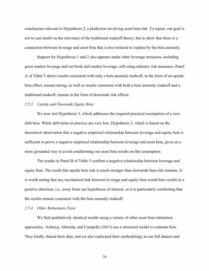
Our main variables are introduced in Table 1. Our basic sample is the portion of the

merged CRSP-Compustat sample for which marginal tax rates are available from John Graham.

The data begin in 1980, when marginal tax rates are first available, and end in 2014. They

contain 1,038,097 firm-months and span all 50 Fama-French (1995) industries. Unlike much

capital structure research, we include financial firms because they are not special under the beta

20

anomaly theory, but their exclusion does not affect the relevant results. In an average cross-

section there are 2,181 profitable and 291 unprofitable firms.

Variable definitions are in Appendix 1. Gross book leverage is long-term debt and notes

payable divided by the sum of long-term debt and notes payable plus book equity. Net book

leverage nets out cash and equivalents from the numerator and denominator. Gross and net

market leverage replace book equity with the market value of common equity from CRSP.

The regressions control for traditional explanatory variables in Bradley, Jarrell, and Kim

(1984), Rajan and Zingales (1995), Frank and Goyal (2009), Campello and Giambona (2013),

and others. The fixed assets ratio, a proxy for financial distress costs, is net property, plant and

equipment divided by total assets. Profitability, which would be positively correlated with

leverage under the standard tradeoff theory but inversely correlated under the Myers and Majluf

(1984) pecking order, is EBIT divided by total assets. Market-to-book assets is known to be

negatively related to leverage, consistent with the need for firms with strong growth

opportunities to avoid having to pass them up (Myers (1977)) as well a more passive lack of

adjustment of leverage to prior stock returns (Welch (2004)). It is gross debt and market equity

divided by the sum of gross debt and book equity. Asset growth could be a proxy for growth

opportunities or capture size or the profitability that helps to make debt-financed acquisitions.

Size, the natural log of book assets, may also proxy for multiple influences. Fama and French

(1992) use it to represent the greater cash flow volatility of smaller firms and their higher

expected costs of financial distress. It will also reflect their lesser access to debt markets. Finally,

Graham’s pre-interest marginal tax rates account for many features of the tax code. As shown by

Graham and Mills (2008), these approximate the tax rates simulated with federal tax return data.

21

The leverage determinants that interest us most are constructed from stock returns. Asset

beta is unlevered equity beta, assuming debt is riskless. While betas on corporate debt are very

low, they are difficult to observe; to avoid the results depending on this assumption we have

Hypothesis 3. Total equity risk is the standard deviation of excess stock returns. Asset risk is the

unlevered version. Industry asset beta and risk are market equity-weighted averages.

2.3. Summary Statistics

Tables 2 and 3 show summary statistics and correlations. Profitable firms are larger and

have higher tax rates. Asset beta is somewhat higher for unprofitable firms, as is total risk, which

we will use as a control variable for financial distress costs. With respect to asset risk, a firm

must be promising and at least on a path to profitability to enter the CRSP-Compustat sample for

the 24 months that we require to compute beta. Becoming unprofitable may be associated with

unexpectedly negative returns; also, firms in variable industries are more likely to find

themselves unprofitable in a given period. The latter logic also applies to beta, on the downside.

Other notable correlations in Table 2 are as follows. Gross and net leverage measures are

loosely correlated enough to consider both as a robustness exercise. We follow tradition and

consider both book and market leverage measures. Asset beta, for the own firm or the industry, is

negatively correlated with tax rates and fixed assets and positively correlated with market-to-

book and size. These correlations are generally small relative to the correlations among the

various risk measures.

2.4. Extreme Leverage

Although firms at the leverage extremes are not uncommon, they are particularly

interesting to consider in light of the beta anomaly because they are where the standard tradeoff

theory is least compelling. In particular, a beta anomaly tradeoff could help to explain some of

22

the low leverage puzzle of Graham (2000). As an example, Linear Technology Corporation

(Nasdaq: LLTC) produces semiconductors with a market capitalization of $7.7 billion as of

December 2012. Despite profitable operations, a pre-interest marginal tax rate of 35% by the

methodology in Graham and Mills (2008), and a cash balance of $1 billion, Linear maintains

negative net debt. One potential explanation for this may be its high asset beta.

While rarer than inexplicably low-leverage firms, a number of profitable firms maintain

high leverage despite little tax benefit. Under a standard tradeoff theory, this amounts to

needlessly tempting a fate of financial distress. An example is Textainer (NYSE: TGH), a firm

that leases and trades marine cargo containers. As of the end of 2012, its market capitalization

was approximately $1.7 billion. It has tangible assets of $3.4 billion and a cash balance of $175

million. Despite a marginal tax rate close to 0%, as a result of front-loaded depreciation, modest

growth, and an offshore tax status, it maintains $2.7 billion in debt. A potential explanation for

this inconsistency with the standard tradeoff theory is the firm’s low asset beta. Under a beta

anomaly, equity is undervalued at low leverage, and its value rises steadily as leverage increases

to its correct valuation, and potentially beyond.

The beta anomaly tradeoff may also be pertinent to a set of uniquely highly leveraged

firms—banks—which are often excluded from capital structure analyses. Figure 3 suggests that a

beta anomaly in equities means that regulating low asset beta firms, in the sense of requiring

them to delever significantly, can impose large increases in the cost of capital and losses in

shareholder value. Baker and Wurgler (2015) find that banks’ asset betas are on the order of

0.10, and that the beta anomaly within banks is at least as large as for all firms. While there are

numerous other forces at play in regulatory debates, the loss of the beta anomaly’s benefits gives

23

a coherent foundation for bankers’ common argument that reducing leverage would increase

their cost of capital.

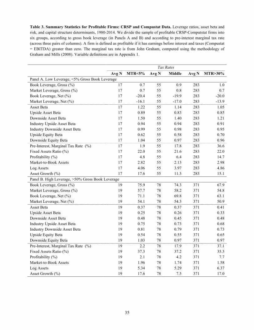
Table 3 looks more closely within profitable firms, where we have 867,524 observations

and the shortcomings of the standard tradeoff theory appear most clearly. The panels separate

profitable firms into low leverage (gross book leverage <5%) and high leverage (gross book

leverage >50%) groups. What counts as high leverage is subjective. We obviously cannot expect

a mode at 100% that resembles the mode at 0%, so we choose an arbitrary cutoff of 50%. The

columns then add another sort into low (MTR<5%), medium, and high (MTR>30%) marginal

tax rate groups.

The low leverage puzzle is represented in the large number of firm-months that have

chosen very low leverage despite positive profitability and high marginal tax rates. In the

average cross-section, not far from half of firms in the highest tax category, 43%, have chosen

low leverage over high leverage (43% = 283/(283+371)). Firms like Linear Technology are here.

The high leverage puzzle, if we can call it that for sake of illustration, is the narrower but still

noticable fact that nearly half of the firms in the low tax category, 47%, have chosen high

leverage (47% = 19/(17+19)). Firms like Textainer are in this bin.

Of course, this is certainly not the only potential driver of extreme leverage. For example,

Denis and McKeon (2012) explain it as an outcome of the evolution of operating needs and the

desire to maintain financial flexibility; see also Hackbarth and Mauer (2011). Hackbarth (2009)

suggests a role for managerial optimism. Regression results follow below, but some initial

support for the beta anomaly tradeoff as an incremental influence comes from the much stronger

differences in asset risk across the leverage levels. Within the middle tax rate group, for example,

asset betas decline sharply with leverage. Firms with very low leverage have a median asset beta

24

of 1.14, a median upside asset beta of 0.83, and a median downside asset beta of 1.40. For high

leverage firms this falls to 0.37, 0.26, and 0.45, respectively.

2.5. Regressions

Turning from extreme leverage observations to the broader cross-section, the first column

in Panel A of Table 4 shows a baseline gross book leverage regression using typical covariates.

We report marginal effects of Tobit regressions that cluster on both firm and month. The first

several variables’ signs and effects are consistent with prior research, as is the poor overall R2.

The marginal tax rate has a positive coefficient, fixed assets a fairly strong positive coefficient,

profitability a negative coefficient, market-to-book a negative coefficient, and size a positive

coefficient. Rajan and Zingales (1995) focus on the latter four variables and obtain the same

results. Asset growth has a positive coefficient, more consistent with the interpretation that asset

growth is a consequence of the ability and desire to finance with debt, determined by other

underlying sources, than an additional proxy for growth opportunities.

2.5.1. Leverage and Asset Beta

We now add risk measures to test Hypothesis 1. Our special focus is on asset beta, which

is what the beta anomaly tradeoff suggests, but we also control for overall risk. In principle, any

effect of total asset risk could reflect the beta anomaly tradeoff—some explanations of the beta

anomaly are specific to beta, others are not. Total asset risk is a plausible proxy for the expected

costs of financial distress, especially compared to asset beta.

The middle columns of Panel A show that asset beta is a strong determinant of leverage,

consistent with Hypothesis 1. This is true controlling for overall asset risk (and in unreported

univariate regressions). Adding the control variables does not significantly affect the coefficient

25

or t-statistic on asset beta. With all controls, a one-unit increase in asset beta reduces leverage by

12.6%, a large effect by the standards of the control variables.

The last columns of Table 4 show that the economic effects remain if we use industry

risk, which is an empirical solution to the issue of any mechanical negative link between

leverage and asset beta created by using leverage itself to unlever equity beta. It appears that any

measurement error introduced by this switch does not appear to greatly affect the coefficients on

beta risk. These regressions provide further support for Hypothesis 1.

2.5.2 Upside and Downside Asset Beta

We turn next to Hypothesis 2. It is clear that high asset beta is associated with lower

leverage. This is consistent with the beta anomaly tradeoff whereby the cost of equity for high

beta assets is lower and so less debt is optimal, but also consistent with versions of the standard

tradeoff theory to the extent that the relationship is driven by downside risk. To examine whether

downside risk alone is driving the relationship, we estimate equity beta separately over months

when the market risk premium was positive and when it was negative. Unlevering these and

averaging by industry gives us an upside asset beta and downside asset beta measure.

In Panel B of Table 4 we find that the upside and downside components of asset beta

have an equally strong relationship to gross book leverage when using the firm’s own risk

measures and the relationship actually favors the upside asset beta under the preferred industry-

based measures. Downside asset beta has no statistical association with leverage and in one case

a point estimate of the wrong sign to support a version of the traditional tradeoff.

Reassuringly for the traditional tradeoff, and consistent with our use of asset risk as a

control variable for financial distress, the downside overall asset risk association with leverage is

generally stronger than the upside asset risk association. This of course does not alter the

26

conclusions relevant to Hypothesis 2, a prediction involving asset beta risk. To repeat, our goal is

not to cast doubt on the relevance of the traditional tradeoff theory, but to show that there is a

connection between leverage and asset beta that is less tortured to explain by the beta anomaly.

Support for Hypotheses 1 and 2 also appears under other leverage measures, including

gross market leverage and net book and market leverage, still using industry risk measures. Panel

A of Table 5 shows results consistent with only a beta anomaly tradeoff, in the form of an upside

beta effect, remain strong, as well as results consistent with both a beta anomaly tradeoff and a

traditional tradeoff, remain in the form of downside risk effects.

2.5.3 Upside and Downside Equity Beta

We now test Hypothesis 3, which addresses the required practical assumption of a zero

debt beta. While debt betas in practice are very low, Hypothesis 3, which is based on the

theoretical observation that a negative empirical relationship between leverage and equity beta is

sufficient to prove a negative empirical relationship between leverage and asset beta, gives us a

more grounded way to avoid conditioning our asset beta results on this assumption.

The results in Panel B of Table 5 confirm a negative relationship between leverage and

equity beta. The result that upside beta risk is much stronger than downside beta risk remains. It

is worth noting that any mechanical link between leverage and equity beta would bias results in a

positive direction, i.e., away from our hypotheses of interest, so it is particularly comforting that

the results remain consistent with the beta anomaly tradeoff.

2.5.4 Other Robustness Tests

We find qualitatively identical results using a variety of other asset beta estimation

approaches. Acharya, Almeida, and Campello (2013) use a structural model to estimate beta.

They kindly shared their data, and we also replicated their methodology in our full dataset and

27

jointly estimated asset volatility with asset beta. Choi (2013) uses an empirical measure of asset

betas by combining the returns of fixed income instruments with equity weighted by their market

values. These approaches all lead to qualitatively identical results to our simple and transparent

estimate of asset betas. The detailed results are available on request.

Finally, in additional unreported robustness tests suggested by referees, we found that

switching to quarterly data (instead of clustering monthly), or expanding the sample by dropping

the requirement to include Graham’s marginal tax rates, had little effect. Dropping total risk or

equity risk in Tables 4 and 5 also had no qualitative impact.

3. Conclusion

Many studies have shown that high-risk equities do not earn commensurately high

returns. This paper derives a novel explanation for leverage that is consistent with this

observation. We show that for firms with relatively risky assets, the cost of capital is minimized

at a low level of leverage. For firms with very low risk assets, low leverage entails a substantial

cost in the form of issuing undervalued equity, and hence the cost of capital is minimized at

much higher levels of leverage. In the data, leverage is indeed inversely related to systematic

risk, supporting the main prediction of the beta anomaly tradeoff.

Importantly, we derive and test a prediction of the beta anomaly tradeoff that allows us to

separate it from a standard tradeoff explanation in which asset beta reflects financial distress

costs. The beta anomaly tradeoff predicts that leverage is inversely related to upside risk, not just

downside risk. This is also confirmed. In some specifications, the relationship between leverage

and upside risk is stronger than the relationship with downside risk.

28

More broadly, we suggest that the beta anomaly tradeoff may help to explain the low and

high leverage puzzles in which leverage choices cannot be easily explained by tax and financial

distress considerations alone. Better understanding the empirical limits of a beta anomaly

tradeoff, and how it complements other realistic explanations for leverage that receive support in

the literature, is an area for future research. And, while the beta anomaly is perhaps the obvious

starting point, fruitful research might also come from investigating the interplay of capital

structure and numerous other stock market anomalies.

29

References Acharya, Viral, H. Almeida, and M. Campello. “Aggregate Risk and the Choice Between Cash and Lines of Credit.” Journal of Finance 68 (2013), pp. 2059-2116.

Almeida, Heitor, T. Philippon. “The Risk-Adjusted Cost of Financial Distress.” Journal of Finance 62 (2007), pp. 2557-2586.

Baker, Malcolm, B. Bradley, R. Taliaferro. “The Low-Risk Anomaly: A Decomposition into Micro and Macro Effects.” Financial Analysts Journal 70 (2014), pp. 43-58.

Baker, Malcolm, B. Bradley, J. Wurgler. “Benchmarks as Limits to Arbitrage: Understanding the Low-Volatility Anomaly.” Financial Analysts Journal 67 (2011), pp. 40-54.

Baker, Malcolm, J. Wurgler. “Market Timing and Capital Structure.” Journal of Fiance 57 (2002), pp. 1-32.

Baker, Malcolm, J. Wurgler. “Do Strict Capital Requirements Raise the Cost of Capital? Bank Regulation, Capital Structure, and the Risk Anomaly.” American Economic Review 105 (2015), pp. 315-320.

Bali, Turan, S. Brown, S. Murray, Y. Tang. “A Lottery-Demand-Based Explanation of the Beta Anomaly.” Journal of Financial and Quantitative Analysis 52 (2017), pp. 2369-2397.

Black, Fischer, M. C. Jensen, M. Scholes. “The Capital Asset Pricing Model: Some Empirical Tests.” In M. C. Jensen, ed., Studies in the Theory of Capital Markets. New York: Praeger (1972), pp. 79-121.

Black, Fischer, M. Scholes, “The Pricing of Options and Corporate Liabilities.” Journal of Political Economy 81 (1973), pp 637-659.

Bradley, Michael, G. Jarrell, E. H. Kim. “On the Existence of an Optimal Capital Structure: Theory and Evidence.” Journal of Finance 39 (1984), pp. 857-878.

Brennan, Michael. “Agency and Asset Pricing.” University of California, Los Angeles, working paper (1993).

Campello, Maurillo, and E. Giambona. “Real Assets and Capital Structure.” Journal of Financial and Quantitative Analysis 48 (2013), pp. 1333-1370.

Cargo, Gerald T. “Comparable Means and Generalized Convexity.” Journal of Mathematical Analysis and Applications 12 (1965), pp. 387-392.

Choi, Jaewon. “What Drives the Value Premium? The Role of Asset Risk and Leverage.” Review of Financial Studies 26 (2013), pp. 2845-75.

30

Denis, David, S. B. McKeon. “Debt Financing and Financial Flexibility: Evidence from Proactive Leverage Increases.” Review of Financial Studies 25 (2012), pp. 1897-1929.

Fama, Eugene, K. R. French. “The Cross-Section of Expected Stock Returns.” Journal of Finance 47 (1992), pp. 427-465.

Fama, Eugene, K. R. French. “Common Risk Factors in the Returns on Stocks and Bonds.” Journal of Financial Economics 33 (1993), pp. 3-56.

Frank, Murray Z., V. K. Goyal, “Capital Structure Decisions: Which Factors Are Reliably Important?” Financial Management 38 (2009), pp. 1-37.

Frazzini, Andrea, L. H. Pedersen. “Betting Against Beta.” Journal of Financial Economics 111 (2014), pp. 1-25.

Goldstein, Itay, D. Hackbarth. “Corporate Finance Theory: Introduction to Special Issue.” Journal of Corporate Finance 29 (2014), pp. 535-541.

Graham, John, “How Big Are the Tax Benefits of Debt.” Journal of Finance 63 (2000), pp. 1901-1941.

Graham, John, C. Harvey. “The Theory and Practice of Corporate Finance: Evidence From the Field.” Journal of Financial Economics 60 (2001), pp. 187-243.

Graham, John, L. Mills. “Simulating Marginal Tax Rates Using Tax Return Data.” Journal of Accounting and Economics 46 (2008), pp. 366-388.

Hackbarth, Dirk, D. C. Mauer. “Optimal Priority Structure, Capital Structure, and Investment.” Review of Financial Studies 23 (2012), pp. 747-796.

Harford, Jarrad, M. Martos-Vila, and M. Rhodes-Kropf. “Corporate Financial Policies in Misvalued Credit Markets.” University of Washington working paper (2015).

Hong, Harrison, D. Sraer. “Speculative Betas.” Journal of Finance 71 (2016), pp. 2095-2144.

Long, Michael S., I. Malitz. “Investment Patterns and Financial Leverage.” In: Corporate Capital Structures in the United States, Benjamin M. Friedman, ed. (1985), pp. 325-352.

Merton, Robert C. “On the Pricing of Corporate Debt: The Risk Structure of Interest Rates.” Journal of Finance 29 (1974), pp. 449–470.

Myers, Stewart, N. Majluf. “Corporate Financing and Investment Decisions When Firms Have Information That Investors Do Not Have.” Journal of Financial Economics 13 (1984), pp. 187-221. Myers, Stewart. “Determinants of Corporate Borrowing.” Journal of Financial Economics 5 (1977), pp. 147-175.

31

Rajan, Raghuram, L. Zingales. “What Do We Know about Capital Structure? Some Evidence from International Data.” Journal of Finance 50 (1995), pp. 1421-1460. Shleifer, Andrei, and R. Vishny. “Liquidation Values and Debt Capacity: A Market Equilibrium Approach.” Journal of Finance 47 (1992), pp. 1343-1366. Stein, Jeremy. “Rational Capital Budgeting in an Irrational World.” Journal of Business 69 (1996), pp. 429-455. Welch, Ivo. “Capital Structure and Stock Returns.” Journal of Political Economy (2004), pp. 106-131.

32

Figure 1. Value Effects of Leverage When There is a Beta Anomaly in Equities. We compute firm value for firms with five different levels of asset beta. Each firm has a normally distributed terminal value five years hence, with a contractual distribution of value between debt and equity and no costs of financial distress or tax effects. The value of each firm would be exactly $10, regardless of leverage, if there were no low-beta anomaly. Volatility is equal to asset beta times the sum of a market volatility of 16% plus an idiosyncratic firm volatility of 20%. The risk free rate is 2%. We compute the value of equity, the value of debt, and the equity beta under the Merton model with no beta anomaly. We compound this equity value using the CAPM expected return with a market risk premium of 8% over five years. So, a firm with a beta of 0.25 (beta of 2.0) has a weighted average cost of capital of 4% (18%) in the absence of a beta anomaly. We then present value this future equity value using the discount rate from Equation (1) with a 𝛾 of -5%. This is the adjusted equity value. The weighted average cost of capital uses the adjusted equity value and the value of debt as weights, the cost of equity from Equation (1), and the CAPM for debt. Firm value is the adjusted equity value plus the value of debt. Leverage is computed using these market values. Panel A. Weighted Average Cost of Capital Panel B. Absolute Firm Value

Panel C. Firm Value Relative to the Maximum

33

Table 1. Summary Statistics: CRSP and Compustat Data. Leverage ratios, asset beta and risk, and capital structure determinants, 1980 to 2014. We divide firms into profitable and unprofitable. A firm is defined as profitable if it has earnings before interest and taxes (Compustat = EBITDA) greater than zero. Variable definitions are in Appendix 1. There are 974,470 observations in 50 industries across 420 months.

Profitable Firms Unprofitable Firms Avg N Mean SD Avg N Mean SD

Book Leverage, Gross (%) 2,066 32.7 25.6 255 30.1 33.1 Market Leverage, Gross (%) 2,066 26.8 24.5 255 21.5 25.8 Book Leverage, Net (%) 2,066 21.3 33.4 255 12.9 41.7 Market Leverage, Net (%) 2,066 18.4 29.2 255 8.9 31.6 Asset Beta 2,066 0.71 0.54 255 0.89 0.81 Upside Asset Beta 2,066 0.58 0.56 255 0.58 0.77 Downside Asset Beta 2,066 0.83 0.61 255 1.15 0.99 Industry Upside Asset Beta 2,066 0.79 0.30 255 0.88 0.33 Industry Downside Asset Beta 2,066 0.84 0.30 255 0.93 0.32 Upside Equity Beta 2,066 0.66 0.52 255 0.53 0.60 Downside Equity Beta 2,066 0.96 0.49 255 1.06 0.62 Pre-Interest, Marginal Tax Rate (%) 2,066 33.4 10.3 255 14.0 14.0 Fixed Assets Ratio (%) 2,066 32.4 23.6 255 24.3 22.4 Profitability (%) 2,066 9.7 7.6 255 -21.5 20.4 Market-to-Book Assets 2,066 1.9 1.9 255 3.1 3.9 Log(Assets) 2,066 5.7 2.2 255 3.4 1.8 Asset Growth (%) 2,066 13.8 29.6 255 3.3 46.2

34

Table 2. Correlations: CRSP and Compustat Data. Leverage ratios, asset beta and risk, and capital structure determinants, 1980-2014. Variable definitions are in Appendix 1. There are 974,470 observations in 50 industries across 420 months. Panel A. Leverage Ratios

Book Leverage Market Leverage Gross Net Gross Net Book Leverage, Gross (%) 1.00 Market Leverage, Gross (%) 0.78 1.00 Book Leverage, Net (%) 0.93 0.77 1.00 Market Leverage, Net (%) 0.78 0.93 0.86 1.00

Panel B. Leverage Determinants

Own Asset Risk

Industry Asset Risk

Own Equity Risk

Beta Up Down SD Up Down SD Up Down SD Asset Beta 1.00 Upside Asset Beta 0.87 1.00 Downside Asset Beta 0.93 0.65 1.00 Asset Risk (%) 0.58 0.34 0.66 1.00 Industry Upside Asset Beta 0.37 0.33 0.35 0.29 1.00 Industry Downside Asset Beta 0.34 0.27 0.35 0.30 0.91 1.00 Industry Asset Risk (%) 0.29 0.22 0.29 0.34 0.75 0.83 1.00 Upside Equity Beta 0.62 0.82 0.37 -0.01 0.23 0.17 0.10 1.00 Downside Equity Beta 0.63 0.45 0.69 0.18 0.26 0.28 0.18 0.53 1.00 Risk (%) 0.17 0.02 0.25 0.61 0.23 0.27 0.33 -0.03 0.28 1.00 Pre-Int. Mgl. Tax Rate (%) -0.07 0.01 -0.12 -0.37 -0.12 -0.12 -0.16 0.09 -0.03 -0.47 Fixed Assets Ratio (%) -0.22 -0.16 -0.23 -0.25 -0.28 -0.25 -0.24 -0.06 -0.10 -0.15 Profitability (%) -0.02 0.06 -0.07 -0.30 -0.06 -0.06 -0.09 0.09 -0.05 -0.42 Market-to-Book Assets 0.19 0.15 0.19 0.18 0.18 0.18 0.17 0.10 0.14 0.18 Log(Assets) 0.12 0.28 -0.02 -0.41 -0.11 -0.15 -0.12 0.47 0.16 -0.51 Asset Growth (%) 0.07 0.05 0.08 0.03 0.03 0.05 0.03 0.05 0.10 0.04

35

Table 3. Summary Statistics for Profitable Firms: CRSP and Compustat Data. Leverage ratios, asset beta and risk, and capital structure determinants, 1980-2014. We divide the sample of profitable CRSP-Computstat firms into six groups, according to gross book leverage (in Panels A and B) and according to pre-interest marginal tax rate (across three pairs of columns). A firm is defined as profitable if it has earnings before interest and taxes (Compustat = EBITDA) greater than zero. The marginal tax rate is from John Graham, computed using the methodology of Graham and Mills (2008). Variable definitions are in Appendix 1. Tax Rates

Avg N MTR<5% Avg N Middle Avg N MTR>30% Panel A. Low Leverage, <5% Gross Book Leverage Book Leverage, Gross (%) 17 0.7 55 0.9 283 1.0 Market Leverage, Gross (%) 17 0.7 55 0.8 283 0.7 Book Leverage, Net (%) 17 -20.4 55 -19.9 283 -20.0 Market Leverage, Net (%) 17 -16.1 55 -17.0 283 -13.9 Asset Beta 17 1.22 55 1.14 283 1.05 Upside Asset Beta 17 0.89 55 0.83 283 0.85 Downside Asset Beta 17 1.50 55 1.40 283 1.21 Industry Upside Asset Beta 17 0.94 55 0.94 283 0.91 Industry Downside Asset Beta 17 0.99 55 0.98 283 0.95 Upside Equity Beta 17 0.62 55 0.58 283 0.70 Downside Equity Beta 17 1.04 55 0.97 283 0.96 Pre-Interest, Marginal Tax Rate (%) 17 1.9 55 17.8 283 36.6 Fixed Assets Ratio (%) 17 22.0 55 21.6 283 22.0 Profitability (%) 17 4.8 55 6.4 283 14.7 Market-to-Book Assets 17 2.82 55 2.13 283 2.98 Log Assets 17 4.06 55 3.97 283 4.86 Asset Growth (%) 17 17.6 55 11.3 283 15.1 Panel B. High Leverage, >50% Gross Book Leverage Book Leverage, Gross (%) 19 75.9 78 74.3 371 67.9 Market Leverage, Gross (%) 19 57.7 78 58.2 371 54.8 Book Leverage, Net (%) 19 71.1 78 69.8 371 63.1 Market Leverage, Net (%) 19 54.1 78 54.3 371 50.9 Asset Beta 19 0.37 78 0.37 371 0.41 Upside Asset Beta 19 0.25 78 0.26 371 0.33 Downside Asset Beta 19 0.48 78 0.45 371 0.48 Industry Upside Asset Beta 19 0.75 78 0.73 371 0.68 Industry Downside Asset Beta 19 0.81 78 0.79 371 0.73 Upside Equity Beta 19 0.54 78 0.55 371 0.65 Downside Equity Beta 19 1.03 78 0.97 371 0.97 Pre-Interest, Marginal Tax Rate (%) 19 2.2 78 17.9 371 37.1 Fixed Assets Ratio (%) 19 37.3 78 37.2 371 35.3 Profitability (%) 19 2.1 78 4.2 371 7.7 Market-to-Book Assets 19 1.96 78 1.74 371 1.58 Log Assets 19 5.34 78 5.29 371 6.37 Asset Growth (%) 19 17.6 78 7.5 371 17.0

36

Table 4. Capital Structure and Asset Risk, 1980-2014. Tobit regressions of gross book leverage on capital structure determinants. Gross leverage ratio is defined as long-term debt (DLTT) plus notes payable (NP) divided by long-term debt plus notes payable plus book equity. Book equity is computed in the same way as in Ken French’s data library. Regressions labeled “Own Risk Measures” use firm measures of asset beta and asset risk. Regressions labeled “Industry Risk Measures” use matched Fama-French industry measures of asset beta and asset risk. Other variable definitions are in Appendix 1.

Base Own Risk Measures Industry Risk Measures

Coef [t] Coef [t] Coef [t] Coef [t] Coef [t]

Panel A. Asset Beta Asset Beta -11.6 [-13.0] -12.6 [-10.6] -15.8 [-4.5] -9.4 [-2.5] Asset Risk (%) -2.74 [-16.7] -2.65 [-13.3] -2.39 [-2.6] -2.44 [-2.4] Pre-Interest Marginal Tax Rate (%) 0.11 [2.4] -0.11 [-3.0] 0.06 [1.4] Fixed Assets Ratio (%) 0.19 [4.1] 0.05 [1.6] 0.14 [3.5] Profitability (%) -0.40 [-8.2] -0.46 [-13.5] -0.39 [-8.2] Market-to-Book Assets -1.4 [-5.7] -0.3 [-1.3] -1.1 [-5.0] Log Assets 2.8 [8.8] 2.0 [6.4] 2.6 [10.3] Asset Growth (%) 0.04 [4.4] 0.06 [9.4] 0.04 [4.7] Two-Way Clustering Yes Yes Yes Yes Yes Industries 50 50 50 50 50 Months 420 420 420 420 420 N (000) 974 974 974 974 974 Panel B. Upside and Downside Asset Beta Upside Asset Beta -6.4 [-10.7] -8.1 [-11.7] -14.7 [-5.2] -12.7 [-3.9] Downside Asset Beta -8.2 [-12.4] -7.5 [-12.1] -0.3 [-0.1] 5.1 [1.5] Upside Asset Risk (%) -1.71 [-4.7] -0.69 [-1.4] -3.55 [-1.0] 4.84 [1.1] Downside Asset Risk (%) -3.15 [-6.3] -4.06 [-8.2] -3.07 [-0.9] -12.22 [-3.0] Controls Yes Yes Yes Yes Yes Two-Way Clustering Yes Yes Yes Yes Yes Industries 50 50 50 50 50 Months 420 420 420 420 420 N (000) 974 974 974 974 974

37

Table 5. Alternate Leverage Ratios and Equity Beta, 1980-2014. Tobit regressions of leverage on capital structure determinants. We repeat the regression of the third column of Table 4, Panel B, using four different measures of leverage. Net leverage ratios deduct cash and equivalents from debt. Market leverage ratios replace book equity with market capitalization, equal to price times shares outstanding from CRSP. Panel B replaces asset measures of beta and risk with equity measures of beta and risk.

Gross Leverage (%) Net Leverage (%)

Book Market Book Market

Coef [t] Coef [t] Coef [t] Coef [t] Panel A. Upside and Downside Asset Beta Upside Asset Beta -8.1 [-11.7] -8.4 [-12.0] -13.1 [-11.3] -12.6 [-13.7] Downside Asset Beta -7.5 [-12.1] -8.0 [-13.3] -16.5 [-12.9] -16.3 [-15.5] Upside Asset Risk (%) -0.69 [-1.4] -1.05 [-2.7] -3.99 [-7.8] -4.50 [-10.4] Downside Asset Risk (%) -4.06 [-8.2] -3.36 [-7.9] -8.70 [-12.9] -7.86 [-15.9] Controls Yes Yes Yes Yes Two-Way Clustering Yes Yes Yes Yes Industries 50 50 50 50 Months 420 420 420 420 N (000) 974 974 974 974 Panel B. Upside and Downside Equity Beta Upside Equity Beta -7.3 [-7.4] -8.1 [-9.6] -10.3 [-6.4] -10.6 [-8.1] Downside Equity Beta 1.5 [1.5] 0.5 [0.7] 0.5 [0.4] -0.1 [-0.1] Upside Equity Risk (%) 5.80 [9.0] 4.84 [8.5] 6.61 [7.9] 5.51 [8.1] Downside Equity Risk (%) -0.99 [-1.5] -0.45 [-0.8] -1.03 [-1.3] -0.48 [-0.8] Controls Yes Yes Yes Yes Two-Way Clustering Yes Yes Yes Yes Industries 50 50 50 50 Months 420 420 420 420 N (000) 974 974 974 974

38

Appendix 1. Variable Definitions. All variables are Winsorized at 1% and 99% as measured across the whole sample.

Asset Beta Equity Beta times one minus net market leverage. Asset Growth The annual change in total assets (AT) divided by total assets one year ago, in percentage terms. Asset Risk (%) Equity Risk times one minus market leverage, net. Book Equity Shareholder’s equity minus preferred stock plus deferred taxes. Shareholder’s equity (SEQ) or the sum

of common equity (CEQ) plus preferred stock (PSTK) if shareholder’s equity is missing or total assets (AT) minus total liabilities (LT) if common equity is missing. Preferred stock is equal to the redemption value of preferred stock (PSTKRV) or the liquidating value of preferred stock (PSTKL) or total preferred stock (PSTK) in that order and set to zero if still missing. Deferred taxes are equal to deferred tax and investment tax credit (TXDITC) or balance sheet deferred tax (TXDB) in that order and zero if missing.

Book Leverage, Gross (%) The sum of total long-term debt (COMPUSTAT = DLTT) and notes payable (NP) divided by the sum of total long-term debt and notes payable and book equity, in percentage terms.

Book Leverage, Net (%) The sum of total long-term debt (COMPUSTAT = DLTT) and notes payable (NP) less cash and equivalents (CHE) divided by the sum of total long-term debt and notes payable and book equity less cash and equivalents, in percentage terms.

Downside Asset Beta Downside Equity Beta times one minus net market leverage. Downside Asset Risk (%) Downside Equity Risk times one minus market leverage, net. Downside Equity Beta Market beta computed from CRSP returns (RET) net of Treasury bill returns (YLDMAT)

from CRSP regressed on the value-weighted market return (VWRET), also net of the Treasury bill return, times an indicator variable when the realized market return is positive and the value-weighted market return times an indicator variable when the realized market return is negative, using three-day overlapping return windows. We require at least 750 overlapping windows of returns and use at most five years of returns. The downside beta is the coefficient on negative market returns.

Downside Equity Risk (%) Standard deviation of CRSP returns (RET) net of Treasury bill returns (YLDMAT), in percentage terms, conditional on the CRSP return (RET) net of the Treasury bill return being negative.

Equity Beta Market beta computed from CRSP returns (RET) net of Treasury bill returns (YLDMAT) from CRSP regressed on the value-weighted market return (VWRET), also net of the Treasury bill return, using three-day overlapping return windows. We require at least 750 overlapping windows of returns and use at most five years of returns.

Equity Risk (%) Standard deviation of CRSP returns (RET) net of Treasury bill returns (YLDMAT), in percentage terms.

Fixed Assets Ratio (%) Plant, property, and equipment, net (PPENT) divided by total assets (AT), in percentage terms.

Industry Asset Beta Market equity weighted average asset beta, computed for each Fama-French industry classification. Market equity is equal to price (PRC) times shares outstanding (CRSP) from CRSP. The 49 industry classifications are defined in Ken French’s data library, with unclassified firms comprising a 50th group.

Industry Asset Risk (%) Market equity weighted average asset risk, computed for each Fama-French industry classification. Market equity is equal to price (PRC) times shares outstanding (CRSP) from CRSP. The 49 industry classifications are defined in Ken French’s data library, with unclassified firms comprising a 50th group.

Log Assets The natural log of total assets (AT). Market-to-Book Assets Sum of total long-term debt (COMPUSTAT = DLTT) and notes payable (NP) and market

equity divided by the sum of total long-term debt and notes payable and book equity. Market equity is equal to price (PRC) times shares outstanding (CRSP) from CRSP.

39

Market Leverage, Gross (%) The sum of total long-term debt (COMPUSTAT = DLTT) and notes payable (NP) divided by the sum of total long-term debt and notes payable and market equity. Market equity is equal to price (PRC) times shares outstanding (CRSP) from CRSP, in percentage terms.

Market Leverage, Net (%) The sum of total long-term debt (COMPUSTAT = DLTT) and notes payable (NP) less cash and equivalents (CHE) divided by the sum of total long-term debt and notes payable and market equity less cash and equivalents. Market equity is equal to price (PRC) times shares outstanding (CRSP) from CRSP, in percentage terms.

Pre-Interest, Marginal Tax Rate (%) John Graham provided estimates of the pre-interest marginal tax rate, computed using the methodology of Graham and Mills (2008), in percentage terms.

Profitability (%) Earnings before interest and taxes (EBIT) divided by assets (AT), in percentage terms. Upside Asset Beta Upside Equity Beta times one minus net market leverage. Upside Asset Risk (%) Upside Equity Risk times one minus market leverage, net. Upside Equity Beta See Downside Beta. The upside beta is the coefficient on positive market returns. Upside Equity Risk (%) Standard deviation of CRSP returns (RET) net of Treasury bill returns (YLDMAT), in

percentage terms, conditional on the CRSP return (RET) net of the Treasury bill return being positive.