level iv honours project 2006 project 323 – 6dof...
TRANSCRIPT

Project 323 – 6DOF Hovering P
Faculty of Engineering, Mathematical and Computer Sciences School of Mechanical Engineering
Authors: Ryan Arbon Elias Arcondoulis Mark Gilmour Ryan Matthews
Supervisor:
Dr Ben Cazzolato Sponsor:


Executive SummaryThis report outlines the design, build and control of a craft capable of stablehover in six degrees of freedom, named the WASP. The thrust is generatedby an electric motor driving a five inch ducted fan and attitude stability isachieved through deflections of aerofoils placed in the fan efflux.
The Dynamax fan to be used was tested to obtain a thrust/speed char-acteristic, which was extrapolated to determine the thrust attainable. Amass budget was established and the fan characteristic analysed to select amotor capable of driving the fan to the speeds required.
The objective of the platform design was to optimise the dynamic per-formance of the craft in hover such that it was most easily controllable.An analysis of the desirable location for craft centre of gravity supportedthe decision to mount the motor in a top drive manner, unconventional tothe particular fan used. This added to the considerable mechanical designchallenges of providing structural rigidity given that thrust limitations ofthe fan placed a strict weight budget on any structural components.
The detailed dynamics of the craft were derived and linearised in orderto form a strategy for full six degree of freedom control. The controller wasformulated from classical control techniques, although other methodologiesare investigated. Thrust vectoring techniques are used to allow commandfollowing in horizontal translation.
Following the construction of the craft a series of system identificationexperiments were devised and conducted to obtain estimates for craft pa-rameters used in the dynamic modelling. These values were verified frommultiple sources where possible, to increase accuracy and validate controllersimulations based on the mathematical model of the craft.
Dynamic testing of the craft commenced on a ball joint configuration,where a yaw controller was tuned, as were gains for feedforward compensa-tion of the gyroscopic moment on both pitch and roll axes. While six axistesting remains incomplete at the time of publishment, the authors endeav-our to achieve stable hover of the craft within a tethered environment.
The project goals were highly ambitious within the time frame availableand although full six degree control has not been achieved there has beena considerable amount of groundwork laid for future work either on theWASP, or a larger similar craft.


iii
AcknowledgementsThe authors would like to express their sincere thanks to the many peoplewho have contributed to the project. We would particularly like to thankthe project supervisor, Dr Ben Cazzolato, for his guidance and assistancethroughout the year. Ben made himself continually available amongst hisbusy schedule which was most appreciated.
The Sir Ross and Sir Keith Smith Fund provided financial support with-out which the project would not have been possible. For this the authorsare sincerely appreciative.
The assistance of postgraduate students Zebb Prime, Rohin Wood andWill Robertson has been invaluable. The authors would like to thank Zebb,whose knowledge from last year’s project saved the group many headaches.Thanks also to Rohin whose depth of knowledge was critical to the for-mualtion and implementation of the control strategy. Will was happy todevote time to the compilation of this report in LATEX which was gratefullyreceived.
Also, all the technicians from the Mechanical Workshop must be thanked,including Richard Pateman and Bill Finch. A special thanks should go toSteve Kloeden. Steve’s practical insight and mechanical skills allowed thedesign and fabrication of a successful platform.
The Instrumentation Workshop has also played a large part in the project.The authors would like to all the staff in the workshop and, in particular, MrSilvio De Ieso whose knowledge in all things electronic assisted the endlesstroubleshooting.
And finally, the authors would like to thank all their families and friendsfor their support throughout the year.


v
DisclaimerWe, the authors, declare that the material contained within is entirely ourwork unless otherwise stated.
.............................................Ryan ArbonDate:
.............................................Elias ArcondoulisDate:
.............................................Mark GilmourDate:
.............................................Ryan MatthewsDate:

Contents
Executive Summary i
Disclaimer v
Contents vii
List of Figures xiii
List of Tables xix
Notation xxi
1 Introduction 11.1 Aim 11.2 Scope 2
2 Literature Review 52.1 Findings of Previous Reports 5
2.1.1 Controllability 52.1.2 Safety 72.1.3 Thrust to Weight Ratio 8
2.2 Concept Analysis 82.2.1 Thrust Vectoring 92.2.2 Propulsion 92.2.3 Thrust Control 112.2.4 Single Drive Designs 122.2.5 Single Drive Actuation 122.2.6 Schlecht’s SADTU 162.2.7 Twin-Drive Counter-Rotors 18
vii

viii Contents
2.2.8 Quad-Drive Units 182.3 Control Methodologies 19
2.3.1 Classical Control 202.3.2 State Space Control 212.3.3 Alternative Methodologies 22
3 Concept Selection & Feasibility Study 253.1 Testing of the Dynamax Ducted Fan 27
3.1.1 Experimental Methods for Measuring Thrust 273.1.2 Test Rig Design 283.1.3 Apparatus 283.1.4 Method 303.1.5 Results 30
3.2 Feasibility Calculations 313.2.1 Untethered Mode 313.2.2 Tethered Mode 34
3.3 Custom Fan Design 35
4 Component Selection 394.1 Propulsion System 39
4.1.1 Ducted Fan 394.1.1.1 Dynamax 404.1.1.2 Byron Pusher 404.1.1.3 Ramtec 414.1.1.4 Selection 41
4.1.2 DC Motor 414.1.3 Electronic Speed Controller 434.1.4 Power Supply 45
4.1.4.1 Sealed Lead Acid (SLA) Batteries 454.1.4.2 Regulated DC Power Supplies 46
4.2 Control Hardware System 474.2.1 Servo Motors 47
4.2.1.1 Background on Servo Motors 474.2.1.2 Estimated Torque Requirements 484.2.1.3 Servo Frequency Response Testing 504.2.1.4 Selection 53
4.2.2 Servo Motor Battery 55

Contents ix
4.2.3 Sensors 564.2.4 Signal Interfacing Hardware 59
4.2.4.1 dSPACE Platform 594.2.4.2 PicoPic Microcontroller 614.2.4.3 Signal Flow 62
5 Dynamics & Modelling 655.1 Vehicle Dynamics, Stability and Controllability 655.2 Mathematical Model 69
5.2.1 Force Balance 695.2.2 Moment Balance 725.2.3 State Model 73
5.2.3.1 State Variables 735.2.3.2 Plant Inputs 735.2.3.3 Pitch Dynamics 745.2.3.4 Roll Dynamics 745.2.3.5 Yaw Dynamics 755.2.3.6 Vertical Displacement Dynamics 755.2.3.7 Servo Actuator Dynamics 755.2.3.8 Rotor Speed Dynamics 76
5.3 Virtual Reality (VR) Model 76
6 Mechanical Design 796.1 Structural Design 79
6.1.1 Fan Rotor System 806.1.2 DC Motor Mount System 836.1.3 Servo Motor Mounts 876.1.4 Control Vane Coupling and Bearing 896.1.5 Ductwork 91
6.1.5.1 Duct Length Optimisation 916.1.5.2 Central Hub 956.1.5.3 Duct Extension 95
6.1.6 Landing Rig 966.2 Commissioning 986.3 Aerodynamic Design 102
6.3.1 Ducted Fan 1026.3.2 Bellmouth Inlet 104
x Contents
6.3.3 Control Vanes 1076.3.4 Duct Length 1146.3.5 Duct Width 1156.3.6 Central Hub 1176.3.7 Duct Exit 1176.3.8 End Cap 1186.3.9 Ground Effects 118
6.4 Tether Design 120
7 System Identification 1237.1 Equipment 123
7.1.1 Six Axis Force Transducer 1237.1.2 Opto-Coupled Pickup Tachometer 124
7.2 Testing Protocols 1267.3 Static Testing 127
7.3.1 Thrust-Speed Characteristic 1287.3.2 Yaw Moment-Speed Characteristic 1297.3.3 Rotor Speed Dynamics 1327.3.4 Control Vane Characteristic 1327.3.5 Servo Motor Dynamics 134
7.4 Dynamic Testing 1347.4.1 Single Axis Testing 1347.4.2 Vehicle Centre of Gravity and Moments of Inertia 136
7.5 Summary of System Parameters 1387.5.1 Static Craft Properties 1387.5.2 Pitch and Roll Parameters 1387.5.3 Yaw Parameters 1397.5.4 Vertical Displacement Parameters 1407.5.5 Servo Actuator Parameters 1407.5.6 Rotor Speed Parameter 140
8 Control Strategy 1418.1 Classical Single Input-Single Output (SISO) Strategy 141
8.1.1 Pitch and Roll Control 1428.1.2 Yaw and Height Control 1448.1.3 Assessment 146
8.2 State Space Control Methodology 146

Contents xi
8.2.1 Optimal Regulator Design 1468.2.2 Command Tracking 1488.2.3 Integral State Feedback 1488.2.4 Modelling Actuator Dynamics 1508.2.5 Completed Model 1508.2.6 Assessment 1528.2.7 Future Work 152
9 Control Implementation 1559.1 Yaw Rate Control 1579.2 Compensation of Gyroscopic Coupling 1589.3 Pitch and Roll Feedback Compensation 1609.4 Unconstrained Testing 161
10 Conclusion 16310.1 Project Definition, Specification and Contract 16310.2 Budgets 16610.3 Issues 16810.4 Future Work 17210.5 Postanalysis 174
Bibliography 177
A SADTU Design Analysis 181
B Dynamax Fan Testing Calculations 189B.1 Thrust/Strain Relationship 189B.2 Natural Frequency Calculation 192
C Air Flow Analysis 195C.1 Compressibility 195C.2 Fully Developed Flow 197
D Control Vane Aerodynamics 201D.1 Control Vane Design 201D.2 Duct Width 207D.3 NACA 0015 Profile Generation 210
E Bellmouth Inlet Optimisation 213


List of Figures
1.1 Photograph of Moller’s Skycar (Moller International, 2006). 21.2 Photograph of the Draganflyer (Drexel, 2006). 3
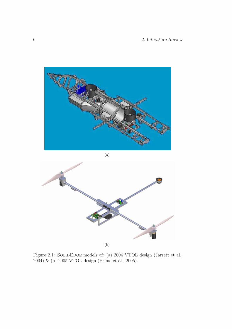
2.1 SolidEdge models of: (a) 2004 VTOL design (Jarrett et al.,2004) & (b) 2005 VTOL design (Prime et al., 2005). 6
2.2 Diagram of the Micro Craft iStar (Lipera et al., 2001). 92.3 Photographs of: (a) V22 Osprey (Philasae, 2006) & (b) Bell
X22 (Prototypes, 2006). 102.4 Photographs of: (a) AROD (White and Phelan, 1991), (b)
GTSpy (Johnson and Turbe, 2005) & (c) iStar (Lipera et al.,2001). 13
2.5 Diagrams of: (a) Control vanes on iStar (Lipera et al., 2001)& (b) Kestrel (Techsburg, 2006). 14
2.6 Diagram of Moller’s Aerobot (1989) showing control vanes(left, yaw and translation control) and spoilers (right, pitchand roll) 15
2.7 Photograph of Moller’s Aerobot Mach I (Moller, 2006). 152.8 Model of the conceptual SADTU, (Schlecht, 2000). 162.9 (a) Model of a counter-rotating prop design (Avanzini and
Matteis, 2006) & (b) Photograph of the Canadair Sentinel(SFU, 2006). 19
2.10 Diagram of a quad rotor design (Hamel et al., 2002). 20
3.1 SolidEdge model of initial concept 263.2 Photograph of the Dynamax 5′′ unit (CRCJA, 2006) 273.3 Photograph of the Plettenberg HP 220-30-A4 brushless DC
motor 283.4 Photograph of the Dynamax fan testing setup 29
xiii

xiv List of Figures
3.5 Diagram of the signal flow for the Dynamax fan test 303.6 Simulink block diagram used in the Dynamax fan test 313.7 Plots of data taken during testing of the Dynamax ducted fan 323.8 Plot of ducted fan thrust/radius characteristic for fixed power
(Exeter, 2006). 363.9 Expected flow chart for the design and manufacture of a cus-
tom ducted fan 38
4.1 Photograph of the 6′′ Byron Pusher (CRCJA, 2006) 404.2 Photograph of the Ramtec unit (left) side by side with the
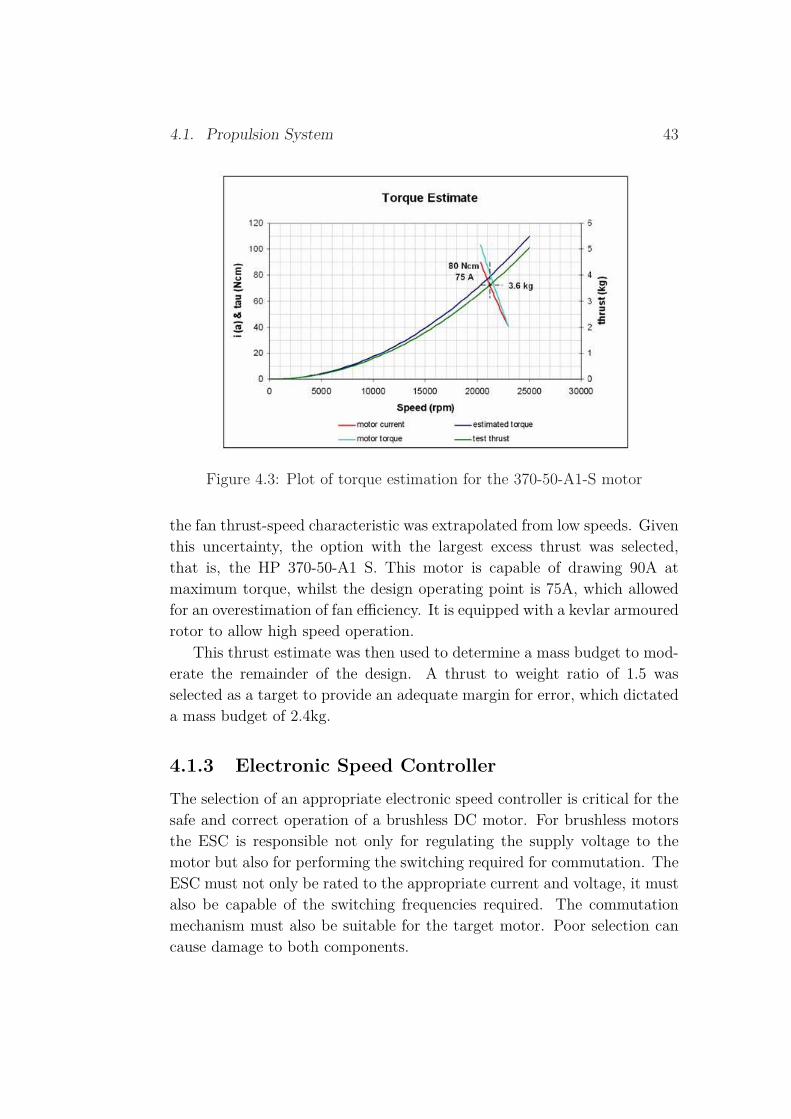
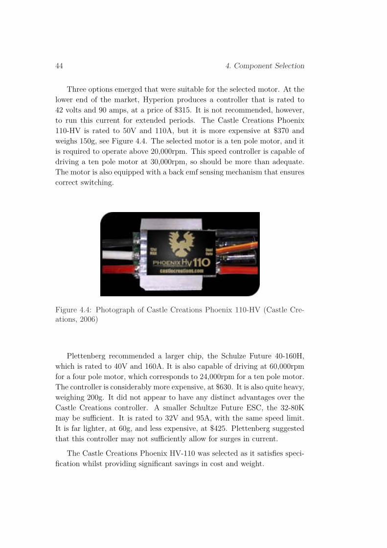
Dynamax (CRCJA, 2006) 414.3 Plot of torque estimation for the 370-50-A1-S motor 434.4 Photograph of Castle Creations Phoenix 110-HV (Castle Cre-
ations, 2006) 444.5 Photograph of the Densei-Lambda power supplies selected 464.6 Illustration of the improved response of digital servos (Futaba,
2006) 494.7 Diagram showing increased signal frequency of digital servos
(Futaba, 2006) 494.8 Diagram of the critical vane locations 504.9 Diagram of a chirp wave form and output oscillating shaft
displacement 504.10 Schematic of servo testing rig 514.11 Plot of the servo frequency responses 524.12 Photograph of a Hitec HS-5475-MG servo motor (Hitec, 2006) 534.13 Plot of the HS-5475 response compared to analogue servo
motors 544.14 Photograph of the servo motor battery 564.15 Diagram of the Logitech Head Tracker sensor showing work-
ing range (Depo, 2006) 574.16 Photograph of the MicroStrain 3DM-GX1 (Microstrain, 2006) 584.17 Photograph of the dSPACE unit 604.18 Simulink model showing an example of dSPACE input/output
references 604.19 ControlDesk graphical output example 614.20 Photograph of the PicoPic microcontroller 624.21 Diagram of hardware interfacing 63

List of Figures xv
4.22 Photograph of the serial connections from the single dSPACEport to both the PicoPic and the IMU sensor 63
5.1 Free body diagram illustrating thrust vectoring & controlvane reaction force 66
5.2 Diagram of different motor/fan configurations 675.3 Free body diagram of a simplified dynamic model 685.4 SolidEdge model of the craft with co-ordinate axes 705.5 Free body diagram for pitch and roll axes 715.6 3D Studio Max 5 model of craft components 775.7 V-Realm Builder 2.0 complete model 78
6.1 SolidEdge model of the motor-fan coupling 816.2 SolidEdge model of the fan rotor bearing 826.3 SolidEdge model of the fan rotor cutaway 836.4 SolidEdge model of the motor mounts (top view) 846.5 SolidEdge model of the motor mounts (side view) 856.6 SolidEdge model of the motor-fan supports 866.7 SolidEdge model of the bottom end assembly 886.8 SolidEdge model of the servo assembly process 896.9 SolidEdge model of the vertical columns 906.10 Photographs of the control vane fixings 916.11 SolidEdge models showing variability in the duct length 936.12 Simulink model used in the duct length optimisation 936.13 Plots of open and closed loop step responses 946.14 Photograph of components assembled inside the acrylic hub 956.15 Photograph of the outside duct fitting into the fan 966.16 SolidEdge model showing the crash envelope 976.17 SolidEdge model of the adapted landing bracket 986.18 SolidEdge model of the independent landing bracket 996.19 Plot of spectra taken at a run speed of 140 Hz 1006.20 Photograph of the capacitor placed in series with the power
supply 1016.21 Plot of spectra taken at a run speed of 140Hz after rebuild 1016.22 Plot of compressible and incompressible thrust-speed schemat-
ics 1036.23 SolidEdge model of the fan rotor, top view 104

xvi List of Figures
6.24 SolidEdge model of the ducted fan inlet 1056.25 Diagram of the inlet conditions: rounded and square edged
Inlets 1056.26 Plot of the bellmouth radius optimisation 1076.27 SolidEdge model showing the control vanes 1086.28 Diagram of the control vane geometric parameters 1086.29 Diagram of the relevant lift and drag coefficients for a NACA
0015 profile (AerospaceWeb, 2006) 1106.30 Diagram of a planform view of predicted and expected flow
patterns 1126.31 Diagram of a side view of predicted and expected flow patterns1126.32 SolidEdge model of the NACA 0015 interpolation 1136.33 Diagram of control vane placement 1146.34 Diagram of duct width analysis 1166.35 Plot of control vane width optimisation (2D Theory) 1166.36 SolidEdge model of the end cap and actual end cap at-
tached to the craft 1196.37 Photograph of ground effects on the iStar (Lipera et al., 2001)1196.38 SolidEdge model of the tether dynamics 1216.39 Photograph of tether cables 121
7.1 Photograph of the six axis force tranducer and strain guageamplifier 124
7.2 Simulink model showing low pass filters applied to the rawtransducer data 125
7.3 Simulink model of the pulse counter algorithm used 1267.4 Photograph of the craft mounted to the six axis force transducer1287.5 Plot of the thrust-speed characteristic 1297.6 Plot of the linearised thrust-speed characteristic about 24N 1307.7 Plots of yaw response to: (a) Ramp speed input, (b) Step
speed input 1317.8 Plot of speed response lag 1327.9 Plot of vane force to angle of attack 1337.10 Plot of second order model against the measured data set 1357.11 SolidEdge model of the single axis rig 1357.12 Plot of craft inertia determined from the pendulum test 137

List of Figures xvii
8.1 Simulink open loop model of the coupled pitch and roll states1428.2 Plot of the open loop pitch and roll responses to a step in pitch1438.3 Simulink model of the pitch and roll controller 1448.4 Plot of the pitch and roll controller response 1458.5 Simulink model of the yaw rate and height controller 1468.6 Plot of the closed loop step response of the yaw-height controller1478.7 Plot of pitch and roll responses to a roll angle command 1498.8 Simulink representation of state model structure (Cazzo-
lato, 2006) 1518.9 Plot of the system response to a roll command in both roll
and pitch states 151
9.1 (a) Free body diagram & (b) Photograph of the craft on theball joint 156
9.2 Plot of regulated yaw rate in comparison to the open loopbehaviour (biased) 158
9.3 Plot of tuning roll compensation for a step in pitch 1599.4 Bode plot of the unconstrained, pinned and scaled pinned
systems 161
A.1 Diagram of the control duct 183A.2 Diagram of a top view of the control duct 184
B.1 Free body diagram of the Dynamax fan testing setup 190B.2 Simplified free body diagram of the Dynamax fan test 192
C.1 SolidEdge model of the rotor with notation used 196C.2 SolidEdge model of the rotor with notation used 198
D.1 Diagrams of control vane forces and geometry 203D.2 Diagram of the lift and drag coefficients for a NACA 0015
profile (AerospaceWeb, 2006) 204D.3 Diagram of the area seen by flow incident to aerofoil 205D.4 Cross-sectional diagram of a continued stator profile 208D.5 Cross-sectional diagrams for narrowing and widening the sta-
tor profile 209D.6 Plot of control vane width optimisation (2D Theory) 210D.7 Plot of aerofoil curvature 211D.8 SolidEdge data points forming the control vane profile 211

xviii List of Figures
D.9 SolidEdge model of the control vanes 212
E.1 Diagram of the bellmouth inlet profile 214E.2 Bellmouth optimisation plot 217

List of Tables
3.1 Extrapolated trend data 33
10.1 Mass budget 16710.2 Component expenses 16810.3 Estimated labour costs 169
E.1 Inlet loss coefficients: Left, dimensionless & Right, D =0.13m (Munson et al., 2002) 215
E.2 Mass benefit 216E.3 SolidEdge bellmouth masses 216E.4 Net mass budget 217
xix


Notation
Acronyms and Abbreviations
CoG Centre of GravityCoP Centre of PressureCRO Cathode Ray OscilloscopeDC Direct CurrentDoF Degree of FreedomESC Electronic Speed ControllerGPS Global Positioning SystemGUI Graphical User InterfaceIMU Inertial Measurement UnitLiPo Lithium PolymerLQR Linear Quadratic RegulatorLTI Linear Time-InvariantOLS Ordinary Least SquaredPID Proportional Integral DerivativePM Permanent MagnetPWM Pulse Width ModulationRC Remote ControlledRPM Revolutions Per MinuteSISO Single Input Single OutputSLA Sealed Lead AcidUAV Unmanned Aerial VehicleVTOL Vertical Take-Off and Landing
xxi

xxii Notation
Nomenclature
Attitude Angular position of an aircraft relative to itsdirection of motion
Pitch Vertical rotation of an aircraft about its axisperpendicular to its direction of motion
Roll Rotation of an aircraft about its axis of motionYaw Left and right rotation of an aircraft about its
axis perpendicular to its direction of motion
Roman Symbols
As used in the body of the report, with seperate notation for appendices.
cf Force constant from vane deflectioncm Moment constant from vane deflectionct Torque constantcth Thrust constantdf Control duct outlet diameter (m)d0 Control duct inlet diameter (m)d1 Central hub diameter (m), fan rotor (m)d2, D Duct diameter (m)f Friction factorF Control vane lift force (N)Fx Force in the x - axis per unit angle in the pitch servo (N)Fy Force in the y - axis per unit angle in the roll servo (N)Fhover Control vane force at hover (N)Fmax Maximum control vane force (N)g Gravitational constant (m/s2)h Central hub diameter (m)hL Head loss (m)JCoG Moment of inertia about the crafts CoG (kgm2)Jfr Fan rotor inertia (kgm2)Jmr Motor rotor inertia (kgm2)JR Moment of inertia of the rotor (kgm2)
Notation xxiii
Js Moment of inertia of the total system about the pivotpoint (kgm2)
Jxx Moment of inertia of entire plant (including rotor)about the roll axis (kgm2)
Jyy Moment of inertia of entire plant (including rotor)about the pitch axis (kgm2)
Jzz Moment of inertia of entire plant (including rotor)about the yaw axis (kgm2)
Kentry Pressure loss coefficient of the duct entryKelbow Pressure loss coefficient of the duct elbowKexit Pressure loss coefficient of the duct exitKlength Pressure loss coefficient of the duct lengthKt Thrust per unit angle in the spoil servo (N/rad)KT Thrust per unit rotor speed at hover (N/(rad/s))lp, lr Distance from CoG of craft to pivot point (m)lθ,φ Control vane moment arm for pitch and roll (m)lψ Control vane moment arm for yaw (m)L Duct length (m)m Linearised lift coefficient (1/rad)M Vehicle mass (kg)MR,θ Pitch gyroscopic coupling coefficient (1/s)MR,φ Roll gyroscopic coupling coefficient (1/s)Mt Thrust (spoil) servo effectiveness (m/s2)MT Rotor thrust effectiveness (m/s)MY Ratio of rotor inertia to body yaw inertia (rad/s)Mθ Pitch servo effectiveness in (1/s2)Mφ Roll servo effectiveness in (1/s2)Mψ Yaw servo effectiveness in (1/s2)∆P Pressure drop (Pa)r Radius (m)t Control vane width (m)T Thrust (N), Period of oscillation (s)Tmax Maximum torque imposed on the servo (Nm)

xxiv Notation
Tθ Pitch torque per unit angle in pitch servo (Nm/rad)Tφ Roll torque per unit angle in roll servo (Nm/rad)Tψ Yaw torque per unit angle in yaw servo (Nm/rad)TΩ Time constant of the motor and speed controller (s)u(r) Velocity profile (m/s)ui Desired servo angle (rad)ut Desired thrust (spoil) servo setting (rad)uθ Desired pitch servo deflection angle (rad)uφ Desired roll servo deflection angle (rad)uψ Desired yaw servo deflection angle (rad)uΩ Desired rotor speed (rad/s)U Air speed (m/s)x x translation (m)y y translation (m)z Vertical displacement (m)
Greek Symbols
α Angle of attack (rad)δ Control vane deflection (rad)δt Thrust (spoil) servo setting (rad)δθ Pitch servo deflection angle (rad)δφ Roll servo deflection angle (rad)δφ Yaw servo deflection angle (rad)ζi Damping coefficient of the servo motorsρ Density (kg/m3)θ Pitch angle (rad)φ Roll angle (rad)ψ Yaw angle (rad)ωi Natural frequency of the servo motor poles (rad/s)ωr, ΩR Rotor speed (rad/s)

Notation xxv
ΩR,0 Rotor speed at hover (rad/s)∆ΩR Change in rotor speed about hover (rad/s)


Chapter 1
Introduction
The Vertical Take Off and Landing Unmanned Aerial Vehicle (VTOL UAV)provides a powerful platform for the demonstration of automatic controltheory and techniques. The capabilities of these aircraft are often limitedonly by the methods that are used to manipulate them, thus it presents achallenging but rewarding project for the student to apply their knowledgeof control.
In recent years, the VTOL concept has expanded far beyond the mannedmilitary class of aircraft from which it emerged. Small scale UAVs havedeveloped into a popular vehicle for field reconnaissance missions. Non-military applications are also emerging. In the manned class, the Skycar(Figure 1.1) developed by Moller International (2006), demonstrates the po-tential of the technology in revolutionising transportation methods. Modelradio controlled (RC) VTOL UAVs have also become commonplace, suchas the Draganflyer (Figure 1.2). The possible commercial applications arelimitless.
1.1 Aim
The aim of this project was to build a six degree of freedom (DOF) VTOLUAV that is capable of stable hover and can be operated in a lab environ-ment. In accordance with its proposed use as a teaching aid, a user friendlyinterface was developed for the rig and for safety reasons the craft will beflown in a tethered configuration.
Whilst untethered flight was not achievable within the time constraints
1

2 1. Introduction
Figure 1.1: Photograph of Moller’s Skycar (Moller International, 2006).
of this project, the design of the craft was be undertaken with the view that awider flight envelope may be pursued at a later date. General specificationsfor this second phase of design are discussed.
1.2 ScopeThe project encompasses the ground up design of the craft consisting ofa complete literature review, concept analysis, concept selection followedby detailed mechanical and electrical design. The primary goal was anambitious one, and a large amount of the allocated time for this project hasbeen dedicated to design and build of the platform followed by the tuningand testing of a capable control system for the craft.
The original project specification was formulated with the view of util-ising control ducts to stabilise the craft. The evidence uncovered in theliterature review produced a strong case for our eventual selection of a dif-ferent concept, based on control vanes in the main duct efflux. The ductedfan used has been inherited from the 2004 VTOL project (Jarrett et al.,2004), and the thrust/speed characteristics of the fan were tested in orderto select a suitable electric motor to power it. From the results of thistesting a suitable motor was purchased.
Craft dynamics were derived in detail, and a complete mathematicalmodel of the generalised system has been formulated. Platform depen-dant parameters from this gereralised model such as the inertia values,thrust/speed characteristics of the fan and servo motor dynamics have been

1.2. Scope 3
Figure 1.2: Photograph of the Draganflyer (Drexel, 2006).
experimentally determined.The completed system model was used for testing a number of control
strategies in a Matlab simulation environment. Both classical and statespace control strategies were developed and a Virtual Reality (VR) modelof the craft was created to aid in visualising the simulations.
Control implementation and tuning was cut short due to time con-straints, however stable hover was achieved while the craft was looselytethered from all sides. This result proves that the designed platform iscontrollable, and further work could be expected to achieve control withina wider flight envelope.


Chapter 2
Literature Review
Recent years have seen rapid advances in the field of Unmanned Aerial Ve-hicles (UAVs). Many concepts have been developed, in both the fixed androtary wing classes. For many applications, vertical take off and landing(VTOL) capabilities are imperative. Demands on storage, mobility, discre-tion and cost have also driven a continual reduction in scale. Small scaleVTOL UAVs are the focus of this investigation. Much work has been doneon these devices and the literature available is abundant and diverse. Care-ful consideration of the options available was required to determine the mostappropriate direction for this project.
2.1 Findings of Previous ReportsThe previous two years have seen two very different approaches to the designof a small scale VTOL aircraft. In 2004, Jarrett et al. utilised twin ductedfans driven by single cylinder combustion engines as shown in Figure 2.1(a).The 2005 design of Prime et al. used open propellers driven by brushlessDC electric motors, see Figure 2.1(b). This project aims to avoid limitationsencountered in these designs.
2.1.1 Controllability
Combustion engines introduce unsteady power characteristics which areinherent to their method of operation. This is because subtly changingconditions within the fuel mixture such as air moisture content introduce
5
6 2. Literature Review
(a)
(b)
Figure 2.1: SolidEdge models of: (a) 2004 VTOL design (Jarrett et al.,2004) & (b) 2005 VTOL design (Prime et al., 2005).

2.1. Findings of Previous Reports 7
non-linearities. Since fuel is continuously burnt, the mass and thrust char-acteristics of the system are not constant and an adaptive controller wouldbe required to account for these effects. Electric motors have an almost lin-ear relationship between the input voltage and the thrust produced. Sincesystem parameters do not drift, linear controllers will be more successful.This characteristic is particularly advantageous for a platform that is to beused as a teaching aid, since control coursework for undergraduate studentsis all based on linear control theory. Combustion engines are also slowerto respond to a change of setpoint and require continual tuning to sustainmaximum power output. The exhaust from combustion engines combinedwith excessive noise also pose as problems. Electric motors also produceless vibration, allowing lighter frames to be developed and also reducingsensor noise (Jarrett et al., 2004). It would appear that for this project, thecombustion engine may not be the most suitable option, particularly if it isintended to be used as a teaching aid.
2.1.2 Safety
The use of the platform as a teaching aid dictates that safety requirementsbe a primary concern. The two main options for thrust generation were aducted fan or an open propeller and the relative level of safety achievablediffers greatly between the two.
A ducted fan has the rotor enclosed within the duct, preventing acci-dental contact with the blades. If the vehicle was to become unstable, itwould be very unlikely to cause injury to observers. The only potentialhazards are in the case of the rotor detaching itself from the motor or if anobject protrudes into the rotor itself. The latter case can be totally avoidedby a simple screening around the duct entrance if necessary, hovewer theflight environment is to be well controlled and potential hazards can easilybe removed. The former was addressed in the design of a robust motor-fancoupling.
Open propellers are inherently much more dangerous. The exposed pro-pellers are a potential threat, particularly at high speeds when the rotortip cannot be easily seen. Exposed propellers are not suitable for indooruse and would not be recommended for use as part of a teaching aid. Anexample of the danger associated with propellers was exposed in the 2005project, where the propeller shaft sheared during a crash when the blade
8 2. Literature Review
tip contacted the ground (Prime et al., 2005).It was expected that at high fan speeds, the acoustic noise emitted from
the fan will be sufficiently loud such that hearing protection will need tobe worn by anyone in the proximity of the craft. During testing the craftwas operated remotely from behind a solid door such that the sound wassomewhat dissipated. The general safety level could also be increased byoperating the craft behind a perspex shield to minimise both the risk ofphysical contact and hearing damage.
2.1.3 Thrust to Weight Ratio
Operational VTOL aircraft have traditionally been large scale designs in theorder of magnitude of small aircraft. The VTOL projects conducted at theUniversity of Adelaide have been much smaller in scale and as such are moresensitive to thrust to weight ratios. The choice of motor/fan combinationis critical to the thrust to weight ratio achievable. The past projects werereviewed to gauge their findings.
The powerplant for the 2004 project was the OS 91 combustion enginedriving a five inch Dynamax ducted fan. When the system was configured tomaximise thrust (2 tuning pipes, 7 minute flight time, puffer and fuselage),the thrust to weight ratio was 1.55:1 (Jarrett et al., 2004). The 2005 projectwas powered by 220-30-A3-P4 Plettenberg brushless DC motors driving 21inch APC propellers. When the rig was powered by a sealed lead-acid bat-tery, 49N of thrust was generated which gave a thrust to weight ratio of1.27:1 (Prime et al., 2005). This data suggests that combustion engines willprovide a significant advantage in thrust to weight ratio when compared toelectric motors. When comparing thrust to weight ratios, the figures consid-ered were obtained from final conditions, i.e., conditions of the completedfinal design of the respective projects.
2.2 Concept Analysis
Small scale VTOL UAVs have seen many embodiments, with variations inthe methods of propulsion and lift, thrust and attitude control. A funda-mental principle common to all, however, is the principle of thrust vectoring.
2.2. Concept Analysis 9
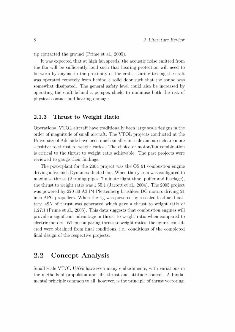
2.2.1 Thrust VectoringThrust vectoring is the basic operating principle of the helicopter that allowsboth vertical take off and landing and forward flight. This concept utilisesthe thrust produced by the propulsion plant to provide lift, longitudinal andlateral propulsion by controlling the direction of this thrust vector. Thisis achieved by either tilting the rotor relative to the vehicle, or controllingvehicle attitude, as is the case for most small scale UAVs (Lipera et al.,2001), see Figure 2.2.
Figure 2.2: Diagram of the Micro Craft iStar (Lipera et al., 2001).
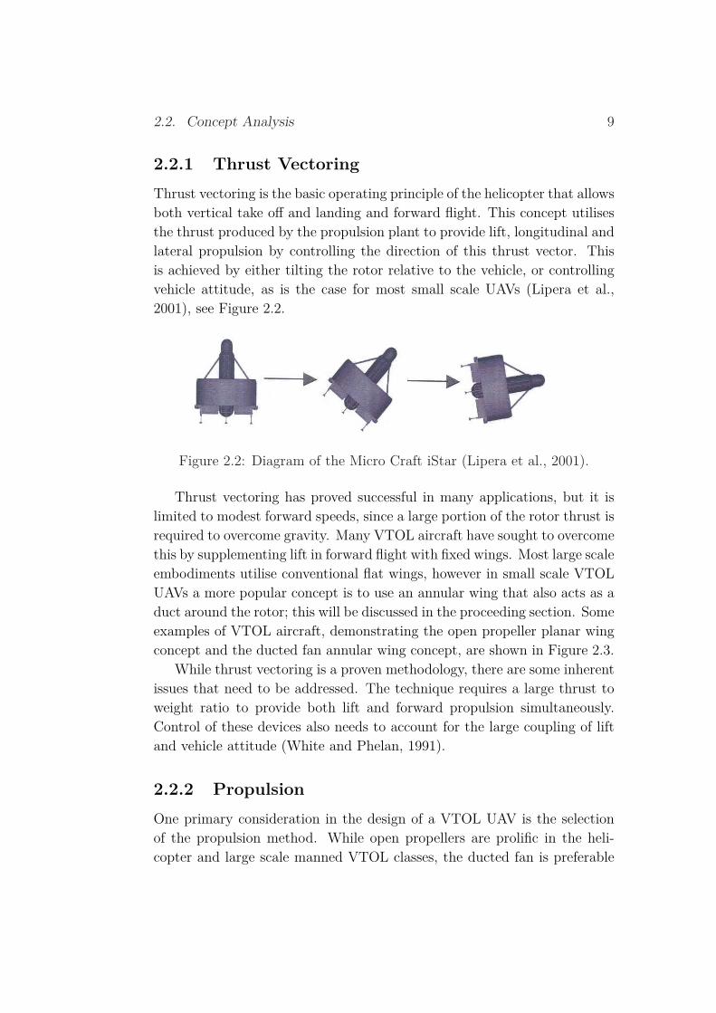
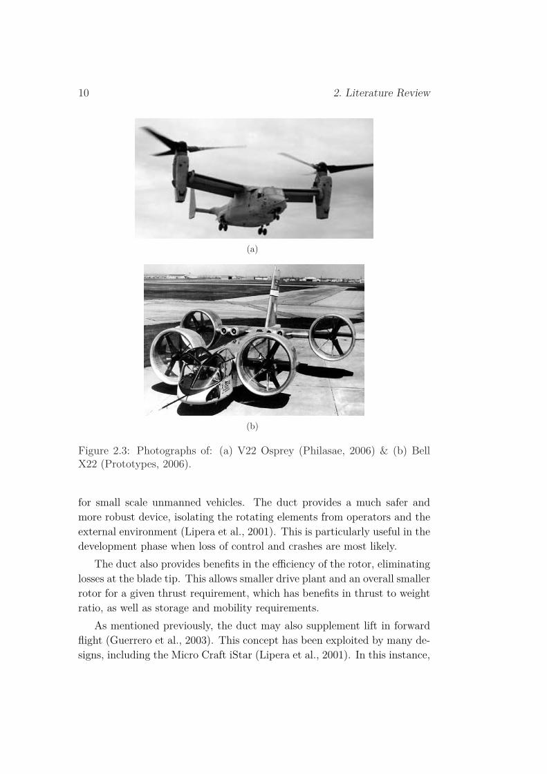
Thrust vectoring has proved successful in many applications, but it islimited to modest forward speeds, since a large portion of the rotor thrust isrequired to overcome gravity. Many VTOL aircraft have sought to overcomethis by supplementing lift in forward flight with fixed wings. Most large scaleembodiments utilise conventional flat wings, however in small scale VTOLUAVs a more popular concept is to use an annular wing that also acts as aduct around the rotor; this will be discussed in the proceeding section. Someexamples of VTOL aircraft, demonstrating the open propeller planar wingconcept and the ducted fan annular wing concept, are shown in Figure 2.3.
While thrust vectoring is a proven methodology, there are some inherentissues that need to be addressed. The technique requires a large thrust toweight ratio to provide both lift and forward propulsion simultaneously.Control of these devices also needs to account for the large coupling of liftand vehicle attitude (White and Phelan, 1991).
2.2.2 PropulsionOne primary consideration in the design of a VTOL UAV is the selectionof the propulsion method. While open propellers are prolific in the heli-copter and large scale manned VTOL classes, the ducted fan is preferable
10 2. Literature Review
(a)
(b)
Figure 2.3: Photographs of: (a) V22 Osprey (Philasae, 2006) & (b) BellX22 (Prototypes, 2006).
for small scale unmanned vehicles. The duct provides a much safer andmore robust device, isolating the rotating elements from operators and theexternal environment (Lipera et al., 2001). This is particularly useful in thedevelopment phase when loss of control and crashes are most likely.
The duct also provides benefits in the efficiency of the rotor, eliminatinglosses at the blade tip. This allows smaller drive plant and an overall smallerrotor for a given thrust requirement, which has benefits in thrust to weightratio, as well as storage and mobility requirements.
As mentioned previously, the duct may also supplement lift in forwardflight (Guerrero et al., 2003). This concept has been exploited by many de-signs, including the Micro Craft iStar (Lipera et al., 2001). In this instance,
2.2. Concept Analysis 11
the duct is formed by a revolved aerofoil profile, thereby acting as an annularwing when tilted in forward flight. This allows for higher angles of attack,which in turn allows for a larger propulsion vector and higher speeds. Insmall UAVs, the duct may also act as the main structural member housingthe vehicle components.
The other main component in the propulsion plant is the motor. Drivemay be provided by either an internal combustion engine or a DC electricmotor. Combustion engines are most commonly used, largely because oftheir distinct advantage in specific power. While battery technology con-tinues to advance, combustion remains the lightest option. Combustionengines are however prone to high levels of vibration, which may corruptsensor readings, as found by the 2004 project. Lipera et al. (2001) overcamethis problem by mounting the engine on vibration isolators. The other mainadvantage of DC electric motors is their capacity for fine speed control athigh speeds and torques. While combustion engines require servo-driventhrottle control, DC motors are electronically controlled. The response ofDC motors is also far more predictable, leading to greater controllability.
2.2.3 Thrust Control
In rotary wing aircraft, one of the fundamental design concepts is the mech-anism of thrust control. This is particularly important for VTOL aircraft,since rotor thrust provides the majority of lift during forward flight andall of the lift during hover, landing and takeoff. There are several differingmethods of thrust vectoring that are commonly used. The most obviousmethod controls thrust by varying the speed of the rotor, making use of theparabolic relationship between the two. Where a constant engine speed isdesirable for efficiency or large rotor inertia limits speed control, other meth-ods are adopted. Most helicopter designs use variable pitch rotors whichcontrol the angle of attack of the rotor blades. Another option utilisedby Schlecht (2000) is to vary the cross sectional area of the duct efflux,essentially choking the airflow.
For the small scale UAV application, variable pitch rotors are not prac-tical. The actuators required to achieve this are complicated, heavy andrealistically not necessary (Moller, 1989). The variable efflux aperture con-cept not only detracts from propulsion efficiency, it introduces inherentuncertainty. Thrust-speed characteristics are known to follow a parabolic
12 2. Literature Review
trend which is easily determined by testing. As discussed previously, brush-less DC motors allow for excellent speed control. Since the size of the fanblades are small, the rotor inertia will be minimal and will not pose controlproblems.
2.2.4 Single Drive Designs
Single drive designs such as the single ducted fan units offer a number ofadvantages. Firstly, the footprint of the vehicle may be very small, onlyslightly exceeding the rotor disc area (White and Phelan, 1991). Mass ofdrive components may also be minimised. However, the most relevant ad-vantage to this project, and many others, is the significant cost advantagein running a single propulsion unit. Given that the motor, fan and speedcontroller constitute a large proportion of the total vehicle cost, this con-sideration is significant in concept selection.
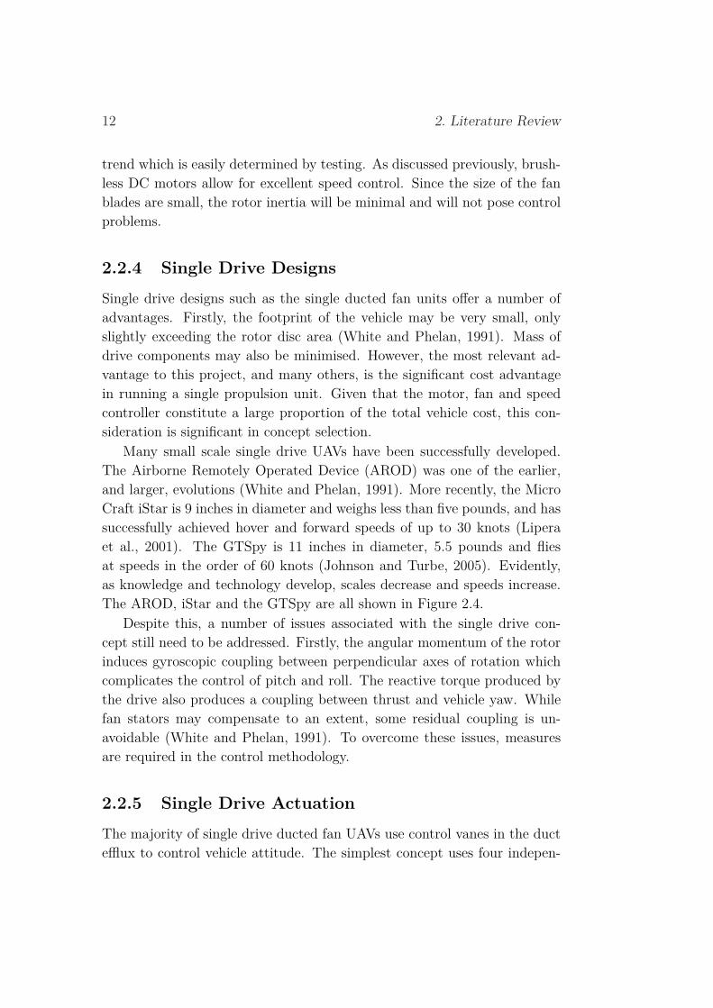
Many small scale single drive UAVs have been successfully developed.The Airborne Remotely Operated Device (AROD) was one of the earlier,and larger, evolutions (White and Phelan, 1991). More recently, the MicroCraft iStar is 9 inches in diameter and weighs less than five pounds, and hassuccessfully achieved hover and forward speeds of up to 30 knots (Liperaet al., 2001). The GTSpy is 11 inches in diameter, 5.5 pounds and fliesat speeds in the order of 60 knots (Johnson and Turbe, 2005). Evidently,as knowledge and technology develop, scales decrease and speeds increase.The AROD, iStar and the GTSpy are all shown in Figure 2.4.
Despite this, a number of issues associated with the single drive con-cept still need to be addressed. Firstly, the angular momentum of the rotorinduces gyroscopic coupling between perpendicular axes of rotation whichcomplicates the control of pitch and roll. The reactive torque produced bythe drive also produces a coupling between thrust and vehicle yaw. Whilefan stators may compensate to an extent, some residual coupling is un-avoidable (White and Phelan, 1991). To overcome these issues, measuresare required in the control methodology.
2.2.5 Single Drive Actuation
The majority of single drive ducted fan UAVs use control vanes in the ductefflux to control vehicle attitude. The simplest concept uses four indepen-

2.2. Concept Analysis 13
(a)
(b) (c)
Figure 2.4: Photographs of: (a) AROD (White and Phelan, 1991), (b)GTSpy (Johnson and Turbe, 2005) & (c) iStar (Lipera et al., 2001).

14 2. Literature Review
dent vanes spaced perpendicularly as in Figure 2.5. One opposite pair con-trols pitch, the other controls roll, and all four control yaw. This concept isproven, and has a distinct advantage in its mechanical simplicity, resultingin a lightweight, reliable and cost effective solution (Lipera et al., 2001).However, it does have a number of limitations that require careful design toovercome. Yaw control is coupled with pitch and roll, which complicates theoverall control methodology and infers large vane deflection. Large deflec-tion is problematic as vanes have non-linear responses and stall at excessiveangles of attack, causing actuator saturation (Fleming and Jones, 2003).This problem can be minimised with careful placement of both the vanesand the vehicle centre of gravity. This is a complex design issue that willbe discussed in detail in subsequent design sections.
(a) (b)
Figure 2.5: Diagrams of: (a) Control vanes on iStar (Lipera et al., 2001) &(b) Kestrel (Techsburg, 2006).
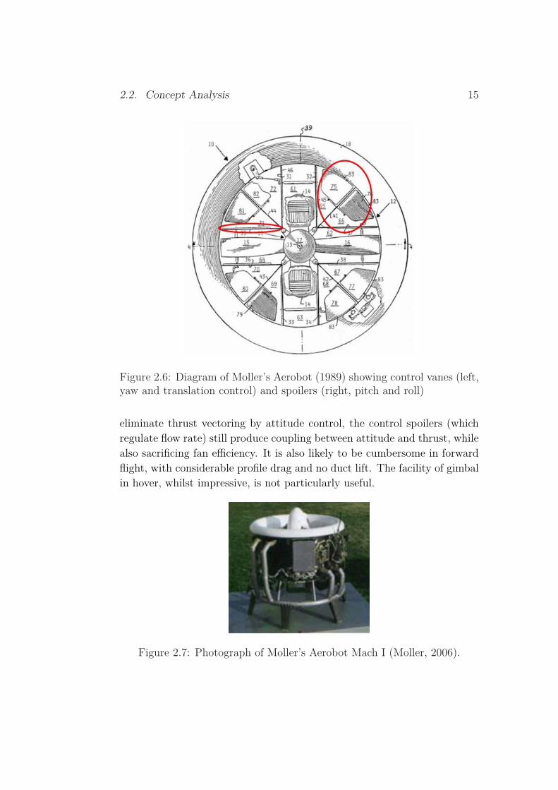
Alternative actuation solutions have sought to overcome these limita-tions. Moller’s first patent (1989) uses more actuators to segregate controlparameters. His design uses flexible vertical vanes to control yaw and lateraltranslation, and independent spoilers to control pitch and roll, see Figure 2.6& Figure 2.7. By designing the flexible vanes such that their centre of pres-sure lies at the centre of gravity, the lateral forces they produce are madeindependent of vehicle attitude. The vanes thereby eliminate the couplingbetween attitude and translation, allowing the vehicle to gimbal in hover.
Moller’s concept has many obvious disadvantages that detract from itsappeal. It is mechanically complex with many actuators, making it heavyand less reliable than simpler solutions. It is also questionable whether themeasures taken actually produce valuable benefits. While the concept does
2.2. Concept Analysis 15
Figure 2.6: Diagram of Moller’s Aerobot (1989) showing control vanes (left,yaw and translation control) and spoilers (right, pitch and roll)
eliminate thrust vectoring by attitude control, the control spoilers (whichregulate flow rate) still produce coupling between attitude and thrust, whilealso sacrificing fan efficiency. It is also likely to be cumbersome in forwardflight, with considerable profile drag and no duct lift. The facility of gimbalin hover, whilst impressive, is not particularly useful.
Figure 2.7: Photograph of Moller’s Aerobot Mach I (Moller, 2006).

16 2. Literature Review
2.2.6 Schlecht’s SADTUAnother alternative concept (Schlecht, 2000) that was investigated in somedetail bleeds airflow from the ducted fan efflux through four lateral controlducts. The ducts exhaust over four servo-controlled aerofoils to generate liftand regulate pitch and roll. Yaw is controlled by variable guide vanes withinthe control ducts. The conceptual design of the Self Automated DynamicThrust Unit (SADTU) is shown in Figure 2.8.
Figure 2.8: Model of the conceptual SADTU, (Schlecht, 2000).
This concept does have the advantage of simplifying the coupling be-tween vehicle attitude and translation, since the aerofoil reaction forces areessentially vertical. However, it is an unproven concept that has severallimitations which raise questions of its viability. The control duct-aerofoilconcept has many inherent uncertainties, since it is dependent on the mainduct velocity profile. There was concern whether sufficient air flow couldbe diverted into the side ducts for attitude control without compromisingthe altitude control the vehicle. Efficiency is also a concern, since flow isdiverted from the main duct which introduces significant frictional lossesin the ductwork. The uncertainties of this design were further investigatedwith a detailed and fully generalised fluid dynamics analysis presented in

2.2. Concept Analysis 17
this report.Basic substitution of parameters into the governing equations of the craft
led to a very important conclusion. It appears that due to the nature of aviscous fluid and the design of the side ducts, the side ducts would receiveinsufficient flow to assert control authority on the vehicle.
A viscous fluid creates a “log law” velocity profile distribution acrossa circular profile, where at the wall the velocity is zero. This is shown inEquation 2.1. Because the control ducts entry points are located on theduct wall, flow entering the ducts is minimal.
u(r) =
√2T
ρπ(d22 − d2
1)(1 + 1.44
√f + 2.15
√f log10(1 − 2r
d2
)) (2.1)
whereu(r)= Velocity profile (m/s)f = Friction factorr = Radius (m)T = Thrust (N)ρ = Density (kg/m3)d1 = Central hub diameter (m)d2 = Duct diameter (m)
One option to overcome this would involve the protrusion of a scoopedprofile duct inlet to improve the control authority. Alternatively the ductinlets could simply be widened. Both of these options would dramaticallyreduce the vertical thrust produced, which compromises the ability to hover.
In addition to the thrust being shared amongst the control ducts, thereare associated losses in each duct. The flow rate required by each ductfor control would have to account for these losses. From the analysis inAppendix A, thrust losses are proportional to the inlet velocity squared asgiven by Equation 2.2. This implies that at higher flow speeds, the efficiencyof the side ducts would decrease.
hL =8π
(∫ d2/2
d2/2−d0/2u(r)dr
)2
d20g
[Kentry +
(d0
df
)2
(Kelbow + Kexit + Klength)
](2.2)
where
18 2. Literature Review
hL = Head loss (m)u(r)= Velocity profile (m/s)d0 = Control duct inlet diameter (m)df = Control duct outlet diameter (m)d2 = Duct diameter (m)g = Gravitational constant (m/s2)Kentry, Kelbow, Kexit, Klength = Pressure loss coefficients of the duct en-
try, elbow, exit and total length respectively
The detailed analysis undertaken has shown that this concept is not fea-sible, given the thrust limitations of the Dynamax fan (refer to Section 3.1)and the inherently low efficiency.
2.2.7 Twin-Drive Counter-RotorsA number of designs utilise twin coaxial counter-rotating rotors to over-come some of the limitations discussed previously. The twin rotor concepteliminates gyroscopic coupling and reactive torque problems, simplifyingcontrol and removing the need for yaw compensation. Yaw control mayalso be achieved by controlling the load share between the two rotors, de-coupling pitch and roll from yaw. This not only simplifies control, but alsoreduces control vane deflection and the associated problems of non-linearityand saturation. While this concept is proven and successfully used in theCanadair Sentinel (Avanzini and Matteis, 2006) and the design of Avanziniand Matteis (2006), it comes at the extra expense of another drive unit, seeFigure 2.9. Potential problems exist regarding swirl between rotors, andwhile some of the control vane issues are addressed, others remain.
2.2.8 Quad-Drive UnitsThe final concept under investigation uses four drive units to control all sixdegrees of freedom, eliminating the need for control vanes. The four rotorsare arranged perpendicularly in the same axial plane. While all contributeto thrust, one pair of opposite rotors controls pitch and the other roll. Speedcontrol of each pair is symmetrical to maintain the desired thrust. The twopairs of rotors rotate in opposite directions to negate gyroscopic effects andreactive torques. Yaw control is provided by controlling the load share

2.3. Control Methodologies 19
(a) (b)
Figure 2.9: (a) Model of a counter-rotating prop design (Avanzini and Mat-teis, 2006) & (b) Photograph of the Canadair Sentinel (SFU, 2006).
between the two pairs of rotors. Figure 2.10 demonstrates this concept.Forward flight is again provided by thrust vectoring by controlling vehicleattitude.
This concept is proven, having been successfully implemented in theDraganflyer (Figure 1.2) and the first evolution of AROD (Figure 2.4(a)).It allows sophisticated and fine control of each degree of freedom, withoutthe problems associated with control vanes. However, it also requires acomplicated control algorithm, since it entails a large degree of couplingbetween thrust and attitude control, which are both controlled by motortorques. The requirement of four drive units makes it a much more expensivesolution, which eliminates it from our consideration.
2.3 Control Methodologies
Various control methodologies have been successfully applied to VTOLcrafts, with different performance results. The task provides a number ofpotential problems that the control methodology must address. There aremany non-linearities associated with thrust vectoring and control vanes andwhich become particularly problematic at high angles of attack. Attitudestability is made difficult because of the inherently unstable open loop dy-namics, resembling that of the inverted pendulum. Ducted fan vehicles arehighly coupled systems with complex flow fields and hence developing anaccurate system model is a difficult task requiring extensive testing (John-

20 2. Literature Review
Figure 2.10: Diagram of a quad rotor design (Hamel et al., 2002).
son and Turbe, 2005). Robustness to unmodelled system dynamics mayalso pose a problem and is to be considered. An examination of the variousmethodologies is required to determine the most appropriate for the presentcontext.
2.3.1 Classical Control
Classical Proportional-Integral-Derivative (PID) control is the simplest ap-proach to the problem, but it accordingly has limitations. This approach isapplicable to linear time-invariant (LTI) systems, so if it is to be applied,approximations are required to linearise the system dynamics, which maycause problems with stability. It is also most commonly applied to single-input, single-output (SISO) systems. As was discussed in Section 2.2.4, thistype of vehicle invariably involves coupling between states such as gyro-scopic coupling between pitch and roll in single-drive units, for instance. APID controller requires a mechanism for decoupling the model states.
The PID control approach has many advantages. There is an abundanceof literature and knowledge available. Many techniques are available to tunethe controllers empirically and there are also many techniques available to

2.3. Control Methodologies 21
examine stability. Many of these tuning techniques, however, are relativelycrude. Accurate pole placement is limited.
PID control was used with good results in Lipera’s iStar (2001). Con-trol gains were optimised with a sophisticated computational software pack-age called CONDUIT (Control Designer’s Unified Interface). A linearisedstate-space model was used to model vehicle dynamics whilst a non-linearsimulation model was used to determine stability and control derivatives.It is encouraging to note that Lipera reported good correlation between thelinear and non-linear models about hover flight conditions. This suggeststhat linearization techniques and PID control may be sufficiently accuratefor a modest flight envelope. At the very least, this approach proved suc-cessful in providing attitude stability during hover, which is the primaryconcern of the control system design. During testing, Lipera reported ade-quate control for relatively aggressive angles of attack, indicating robustnessto non-linearites, albeit with pilot in the loop.
Decoupling of the controller is a problem that can be solved relativelysimply. Lipera uses crossfeeds to reduce the effects of gyroscopic couplingwithin his control system. Another approach presented by Cazzolato (2006)is to develop a decoupling transformation matrix based on the desired con-trol inputs. This approach appears the most systematic.
2.3.2 State Space Control
State Space control provides a more sophisticated and precise alternativethat has been more commonly applied to VTOL UAVs. It allows accurateplacement of all system poles, as well as accurate control of all systemstates, including unmeasured states. While classical transfer functions aredefined only for LTI systems, the State Space approach allows modellingof non-linear, multivariable and time-variant systems (Kuo, 1995). On thenegative side, it is computationally intensive.
The AROD (White and Phelan, 1991) utilises a state space approach tocontrol. The controller includes an integral component to eliminate steadystate error. The performance of the AROD control system provides goodevidence of the capabilities of state control. Whilst the controller design wasbased on a linearised dynamic model, simulation demonstrated robustnessto unmodelled dynamics through highly aggressive manoeuvres.
The biggest difficulty encountered by White and Phelan (1991) was

22 2. Literature Review
gyroscopic coupling, which was exacerbated by limited servo bandwidth.This problem was best mitigated by tuning controller gains with a linear-quadratic-regulator (LQR) approach. This technique is part of the widerapproach of optimal control, which seeks to tune control systems based ona specified performance index. This gives an indication of the scope andsophistication of state space control.
2.3.3 Alternative MethodologiesA number of other, more advanced approaches to UAV control have beentaken to mitigate the limitations of traditional control. These techniquesinclude:
• Partitioned Linearising Control: This approach, which is widely usedin robotics fields, incorporates non-linear dynamics into the controllaw to nullify the effects (Craig, 2005). The plant non-linearity isessentially cancelled from the closed loop system. This is the approachapplied to a ducted fan UAV by Milam and Murray (1999), with soundperformance at high angles of attack.
• Lyapunov Control: For Hamel et al. (2002), traditional approaches arenot adequate for the high degree of coupling in the X4 Flyer (see Sec-tion 2.2.8). Their approach involves a segregated control system witha backstepping controller for rigid body dynamics and a Lyapunovcontroller for the full rotor dynamics. This methodology provides ahighly responsive and stable system capable of highly accurate tra-jectory following. Lyapunov methods also provide stability analysistechniques that are generally applicable, that is, to non-linear andtime variant systems.
• Adaptive Control: Johnson and Turbe (2005) control system includesan adaptive element consisting of a neural network that approximateserror in the dynamic model. This allows for a simplistic model whilstmaintaining a broad flight envelope.
• Robust Control (H∞): Avanzini and Matteis (2006) developed a ro-bust controller based on the H∞ methodology that not only mitigatesunmodeled dynamics and non-linearities, but also limited servo band-width and finite time delays within the system. The performance of

2.3. Control Methodologies 23
the system is greatly improved by integrating two separate controllers,one for low-speed and one for high-speed operating envelopes.
These methods provide considerable advances in performance over tradi-tional approaches to control, facilitating much broader flight envelopes.They are, however, advanced methods that require a large investment oftime for development.


Chapter 3
Concept Selection & FeasibilityStudy
A concept solution was formulated in light of the previous analysis. Thefollowing decisions were made for the following reasons:
Propulsion To be provided by a single ducted fan. The duct providesincreased fan efficiency whilst making the craft safer. It may also havestructural and aerodynamic functions.
Drive The fan was to be driven by a DC electric motor. As was dis-cussed in Section 2.1, DC motors offer numerous advantages in comparisonwith combustion motors. They provide an approximate linear relationshipbetween input voltage and thrust for small deviations about an operatingpoint. They are also less noisy, are less prone to vibration and produce noexhaust fumes. In short, they provide large advantages in predictability andcontrollability of performance.
Attitude Control Attitude control is to be provided by four servo-drivenperpendicular control vanes located in the duct efflux. One opposite pair isto control pitch and the other roll. Yaw is controlled by all four.
Altitude Control There are two mechanisms for altitude control. Fanspeed control can be used to vary the thrust generated. Alternatively, thecontrol vanes may be used to spoil the thrust. The two mechanisms mayalso be used in parallel.
25

26 3. Concept Selection & Feasibility Study
Translation Control Translational control is to be acheived in the samemethod as altitude control, via thrust vectoring.
A SolidEdge model of the concept is shown in Figure 3.1, illustratingthe motor, fan and control vanes.
Figure 3.1: SolidEdge model of initial concept
Power The power requirements of this concept are quite substantial. Ifpossible, power is to be provided by onboard batteries.
Achieving on board power is an ambitious aim that depends largely onthe capabilities of equipment, so a study was undertaken to assess the fea-sibility of this aim. The methodology for the study was as follows. Firstly,an estimate of the thrust achievable with a ducted fan was required. Thiswas to be compared with the mass of the motor and batteries required toproduce this thrust to give an indication of the mass budget available forthe remainder of the craft. An immediate problem was encountered in thatthere is very little published data on commercially available ducted fans.Therefore, to conduct this feasibility study, some empirical data of a ductedfan was required.

3.1. Testing of the Dynamax Ducted Fan 27
3.1 Testing of the Dynamax Ducted FanThis experiment was required to produce a thrust-speed characteristic of aducted fan. The department of Mechanical Engineering provided access toa five inch Dynamax ducted fan as shown in Figure 3.2. This fan typifiesthe range of commercially available fans suitable for this application. Acomparison of commercially available fans is provided in Section 4.1.1. Aswell as determining the feasibility of on-board power, this characteristic alsoformed the basis of motor selection, as described in Section 4.1.2.
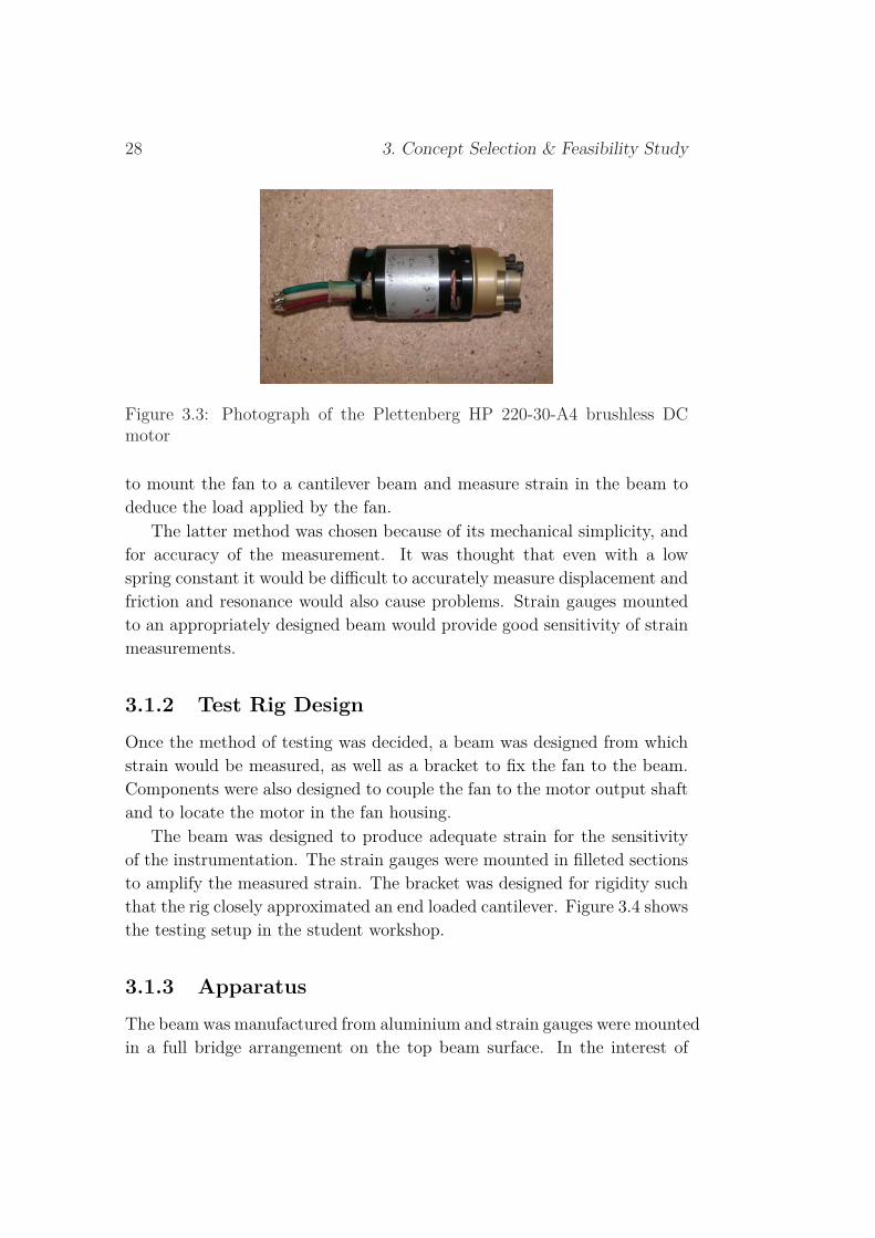
The Plettenberg HP 220-30-A4 brushless DC motor (Figure 3.3) usedfor the 2005 VTOL project (Prime et al., 2005) was used to drive the fanfor this test. The thrust produced was measured for different speeds and aparabolic curve was fit to the results. This motor is capable of only modestspeeds but this was sufficient to produce data from which a curve could beextrapolated.
Figure 3.2: Photograph of the Dynamax 5′′ unit (CRCJA, 2006)
3.1.1 Experimental Methods for Measuring ThrustTwo concepts were investigated for measuring the thrust generated by thefan. The first idea was to measure the thrust by mounting the fan on apivot, where the force generated would be used to compress a spring onthe other end. For a known spring constant, the displacement could bemeasured to calculate the thrust applied by the fan. The other method was
28 3. Concept Selection & Feasibility Study
Figure 3.3: Photograph of the Plettenberg HP 220-30-A4 brushless DCmotor
to mount the fan to a cantilever beam and measure strain in the beam todeduce the load applied by the fan.
The latter method was chosen because of its mechanical simplicity, andfor accuracy of the measurement. It was thought that even with a lowspring constant it would be difficult to accurately measure displacement andfriction and resonance would also cause problems. Strain gauges mountedto an appropriately designed beam would provide good sensitivity of strainmeasurements.
3.1.2 Test Rig DesignOnce the method of testing was decided, a beam was designed from whichstrain would be measured, as well as a bracket to fix the fan to the beam.Components were also designed to couple the fan to the motor output shaftand to locate the motor in the fan housing.
The beam was designed to produce adequate strain for the sensitivityof the instrumentation. The strain gauges were mounted in filleted sectionsto amplify the measured strain. The bracket was designed for rigidity suchthat the rig closely approximated an end loaded cantilever. Figure 3.4 showsthe testing setup in the student workshop.
3.1.3 ApparatusThe beam was manufactured from aluminium and strain gauges were mountedin a full bridge arrangement on the top beam surface. In the interest of

3.1. Testing of the Dynamax Ducted Fan 29
Figure 3.4: Photograph of the Dynamax fan testing setup
safety, the fan was bolted to the end of the beam facing down such that ifthe motor/fan coupling failed, the rotor would fall to the ground rather thaninto the air. The thrust generated produced tensile strain under bending atthe gauges.
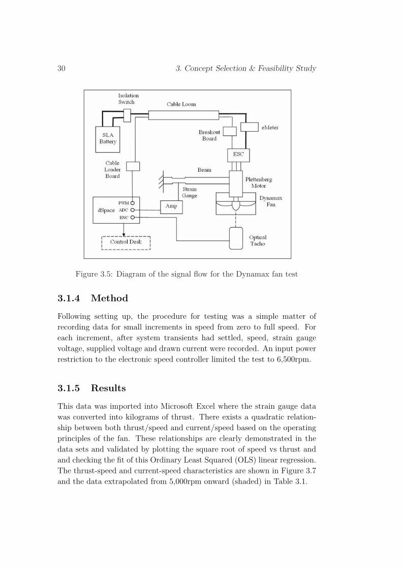
The signal flow diagram is shown in Figure 3.5. The strain gauge signalwas passed through an amplifier where a low pass filter was applied toremove noise from beam resonant modes excited by the drive frequency. Theamplified signal was imported to the dSPACE platform via an analogue-to-digital port where thrust was calculated. This signal was calibrated usingcalibrated masses, the known properties of the beam and the distance ofgauges from the fan.
Fan speed was measured with an optical tachometer, which was mountedon a tripod underneath the fan blades and was also interfaced with dSPACEthrough the digital encoder port.
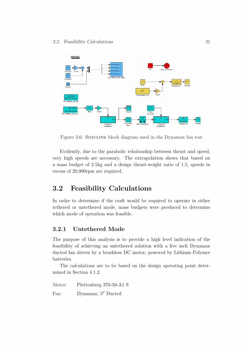
The pulse-width modulation (PWM) signal required to drive the motorwas generated within dSPACE and output from one channel of the PWMport. The signal generated was verified with a cathode ray oscilloscope(CRO). The dSPACE Control Desk platform was used to run the system inreal time, allowing the PWM signal to the motor to be incremented. Thestrain gauge and tacho signals were displayed so speed and thrust couldbe observed and recorded at each speed increment. Figure 3.6 shows theSimulink block diagram used for the test.
The motor was powered at both 13V and 19V by sealed lead-acid (SLA)batteries. A Hyperion eMeter was used to monitor the voltage supplied toand current drawn by the motor.
30 3. Concept Selection & Feasibility Study
Figure 3.5: Diagram of the signal flow for the Dynamax fan test
3.1.4 Method
Following setting up, the procedure for testing was a simple matter ofrecording data for small increments in speed from zero to full speed. Foreach increment, after system transients had settled, speed, strain gaugevoltage, supplied voltage and drawn current were recorded. An input powerrestriction to the electronic speed controller limited the test to 6,500rpm.
3.1.5 Results
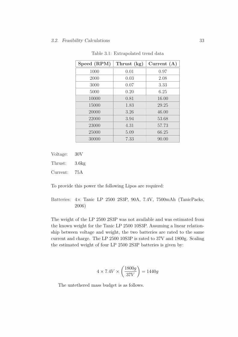
This data was imported into Microsoft Excel where the strain gauge datawas converted into kilograms of thrust. There exists a quadratic relation-ship between both thrust/speed and current/speed based on the operatingprinciples of the fan. These relationships are clearly demonstrated in thedata sets and validated by plotting the square root of speed vs thrust andand checking the fit of this Ordinary Least Squared (OLS) linear regression.The thrust-speed and current-speed characteristics are shown in Figure 3.7and the data extrapolated from 5,000rpm onward (shaded) in Table 3.1.
3.2. Feasibility Calculations 31
Figure 3.6: Simulink block diagram used in the Dynamax fan test
Evidently, due to the parabolic relationship between thrust and speed,very high speeds are necessary. The extrapolation shows that based ona mass budget of 2.5kg and a design thrust-weight ratio of 1.5, speeds inexcess of 20,000rpm are required.
3.2 Feasibility CalculationsIn order to determine if the craft would be required to operate in eithertethered or untethered mode, mass budgets were produced to determinewhich mode of operation was feasible.
3.2.1 Untethered ModeThe purpose of this analysis is to provide a high level indication of thefeasibility of achieving an untethered solution with a five inch Dynamaxducted fan driven by a brushless DC motor, powered by Lithium Polymerbatteries.
The calculations are to be based on the design operating point deter-mined in Section 4.1.2.
Motor: Plettenberg 370-50-A1 S
Fan: Dynamax, 5′′ Ducted

32 3. Concept Selection & Feasibility Study
Figure 3.7: Plots of data taken during testing of the Dynamax ducted fan
3.2. Feasibility Calculations 33
Table 3.1: Extrapolated trend data
Speed (RPM) Thrust (kg) Current (A)1000 0.01 0.972000 0.03 2.083000 0.07 3.335000 0.20 6.2510000 0.81 16.0015000 1.83 29.2520000 3.26 46.0022000 3.94 53.6823000 4.31 57.7325000 5.09 66.2530000 7.33 90.00
Voltage: 30V
Thrust: 3.6kg
Current: 75A
To provide this power the following Lipos are required:
Batteries: 4× Tanic LP 2500 2S3P, 90A, 7.4V, 7500mAh (TanicPacks,2006)
The weight of the LP 2500 2S3P was not available and was estimated fromthe known weight for the Tanic LP 2500 10S3P. Assuming a linear relation-ship between voltage and weight, the two batteries are rated to the samecurrent and charge. The LP 2500 10S3P is rated to 37V and 1800g. Scalingthe estimated weight of four LP 2500 2S3P batteries is given by:
4 × 7.4V ×(
1800g
37V
)= 1440g
The untethered mass budget is as follows.

34 3. Concept Selection & Feasibility Study
Component Mass (g)
Plettenberg 370-50-A1-S 585Speed controller 135Dynamax ducted fan 240LiPo batteries (Plettenberg) 1440LiPo battery (servo & control) 83Servo motors (4×) 180Microcontroller boards* 100IMU sensor 26Chassis** 850
Total mass 3639Net thrust -39
* Estimated value from the 2005 VTOL project (Prime et al., 2005)
** Includes the weight of motor/fan coupling and four control vanes
From this estimation it appears as though untethered flight may not beeasily achievable. Whilst some components may be optimised or upgradedto reduce weight, it is unlikely that this system could achieve a substantialnet positive thrust. Even if stable hover was achieved, there is very littletolerance for thrust vectoring or disturbance rejection. In short, untetheredflight is not feasible with this combination of fan and motor.
3.2.2 Tethered Mode
By deducting the mass of the main power batteries, servo battery and micro-controller boards and including the weight for a short length of lightweightcable, the combination of fan and motor discussed provides more than ad-equate thrust. The tethered mass budget is as follows.

3.3. Custom Fan Design 35
Component Mass (g)
Plettenberg 370-50-A1-S 585Speed controller 135Dynamax ducted fan 240Power cable 60LiPo battery (servo & control) 83Servo motors (4×) 180IMU sensor 26Chassis* 850
Total mass 2159Net thrust +1441
* Includes the weight of motor/fan coupling and four control vanes
This estimate yields a thrust to weight ratio of approximately 1.5.
3.3 Custom Fan DesignTo achieve untethered operation, a more efficient fan is required. Giventhe lack of range in commercially available ducted fans (Section 4.1.1), analternative is to custom design a fan.
The first parameter of interest is the fan radius, which is correlatedwith efficiency. A study by Exeter (2006), proposes a linear relationshipbetween static thrust and radius for a fixed power input, blade profile andnumber of blades (Figure 3.8). Fan mass would also increase with radius,but not substantially. Increasing fan radius has other design implications.It allows for wider control vanes, which not only provides control authoritybut also predictability as large aspect ratio vanes conform more closely tothe two dimensional aerofoil theory. It also implies larger vehicle momentsof inertia, which increases robustness to aerodynamic disturbances. Onthe other hand, a larger fan radius implies a larger rotor inertia, which inturn results in less responsive rotor speed control and a more dominant

36 3. Concept Selection & Feasibility Study
gyroscopic effect. Blade tip speed will also increase for a given rotor speed.This may lead to compressible air flow within the ducted fan, reducingefficiency. However, increasing fan radius would yield a steeper thrust-speedcharacteristic, so this issue may not be relevant.
Figure 3.8: Plot of ducted fan thrust/radius characteristic for fixed power(Exeter, 2006).
The other critical design parameter is the number of rotor blades. Fora fixed rotor radius, increasing the number of blades increases thrust at agiven speed. However, it is also known that rotor efficiency decreases asnumber of blades increases, due to the turbulence created by the leadingblade upstream of the trailing blade. With efficiency in mind, given thecriticality of the thrust to power ratio, a twin blade ducted propeller seemsthe best solution. Twin-bladed ducted propellers are common in VTOLUAVs, including the iStar (Lipera et al., 2001) and the GTSpy (Johnsonand Turbe, 2005).
The design problem, then, is an intricate optimisation problem that re-quires much work. The analysis would require significant mathematical andcomputational analysis and hence a large time frame. The manufacturingprocess would also be extremely intensive, given the complex geometry ofblade profiles. The possibility of constructing a custom fan for the currentproject was deemed unfeasible, due to time constraints.

3.3. Custom Fan Design 37
A proposed design and manufacture process is outlined in Figure 3.9.Both the design and manufacture processes would most likely be iterative.The results generated from a CFD package such as Fluent may give rea-sonable results, empirical testing is also necessary. If the results are notas required, then another iteration would follow. Regardless, the processwould be heavily time consuming and would likely warrant a separate FluidMechanics based project.
An alternative option, which was used by Fleming and Jones (2003),was to develop a duct and stator for a commercially available propeller.This would allow thrust testing to be conducted a priori to select a rotordiameter. The fan stator could then be designed around the propeller.The stator is a critical component of the ducted fan, as it both offsets thereactive torque from the rotor and reduces swirl in the efflux. Without a welldesigned stator, the actuator deflection to balance yaw would be excessive,whilst fan efficiency would be significantly reduced. Design of the statoris a sizeable task in itself, and as such this option was not feasible for thecurrent project.

38 3. Concept Selection & Feasibility Study
Figure 3.9: Expected flow chart for the design and manufacture of a customducted fan
Chapter 4
Component Selection
The first phase of design required the selection of the components whichform the basis of the vehicle. These components can be categorised into twomain functional systems, namely, the propulsion system and the actuationsystem.
4.1 Propulsion SystemThe propulsion system is required to generate the vehicle’s thrust. It com-prises of the ducted fan, the DC brushless motor, the electronic speed con-troller and the motor power supply. Primarily, this system was designedto achieve a thrust to weight ratio greater than one, which is of courserequired to achieve vertical translation. Excess thrust is also required forthrust vectoring, as the vertical component of thrust vector will decrease asthe vehicle tilts. It is also required for disturbance rejection. The larger theratio, higher the saturation limit on thrust and the better the disturbancerejection capability. The available thrust also dictated the mass budget forthe remainder of the design, so a larger ratio provides greater flexibility indesign. In short, the thrust to weight ratio of this system was required tobe maximised.
4.1.1 Ducted FanAs mentioned in Chapter 3, the School of Mechanical Engineering owneda Dynamax ducted fan which was available for use. Other commerciallyavailable ducted fans were researched and compared against this fan.
39
40 4. Component Selection
4.1.1.1 Dynamax
This fan is an 11 blade, five inch diameter unit, shown in Figure 3.2. Themain advantage of this fan is that unlike many other RC fans commonlyavailable, the stator vanes have been designed to counter the rotor reactivetorque. This will greatly reduce the yaw demand and deflections of thecontrol vanes. The balanced stator also straightens the air flow coming outof the fan which is essential for the effective use of control vanes mountedin the duct efflux.
The construction is more precisely manufactured from carbon fibre plas-tics and its price tag reflects its generally superior build quality to the othercommercially available units.
4.1.1.2 Byron Pusher
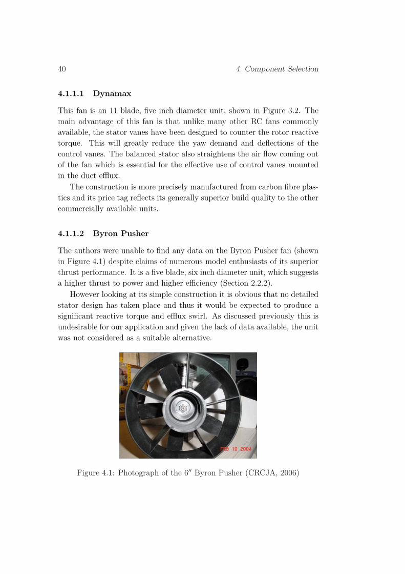
The authors were unable to find any data on the Byron Pusher fan (shownin Figure 4.1) despite claims of numerous model enthusiasts of its superiorthrust performance. It is a five blade, six inch diameter unit, which suggestsa higher thrust to power and higher efficiency (Section 2.2.2).
However looking at its simple construction it is obvious that no detailedstator design has taken place and thus it would be expected to produce asignificant reactive torque and efflux swirl. As discussed previously this isundesirable for our application and given the lack of data available, the unitwas not considered as a suitable alternative.
Figure 4.1: Photograph of the 6′′ Byron Pusher (CRCJA, 2006)

4.1. Propulsion System 41
4.1.1.3 Ramtec
The Ramtec is also an 11 blade, five inch fan. The Ramtec and Dynamaxfans are very similar except that the Ramtec has a larger blade pitch anglewhich suggests greater thrust generated at a given speed. The two units areshown side by side in Figure 4.2. However, without any data to substantiatethis it would seem unwise to spend the $260 on a fan that is so similar toone that the department owns.
Figure 4.2: Photograph of the Ramtec unit (left) side by side with theDynamax (CRCJA, 2006)
4.1.1.4 Selection
Given that there is no obviously superior alternative, the Dynamax ductedfan was selected.
4.1.2 DC Motor
Two main types of DC motor are available for this scale of application,namely brushed and brushless motors. In brushed motors, commutation isprovided by means of mechanical brushes whilst in brushless motors it isprovided electronically by the electronic speed controller. Brushed motorsare less efficient due to brush losses and also deteriorate with time. Thebrushless motors available in the RC market provide the best performancefor this type of application, given the smale scale. Within this market, Plet-
42 4. Component Selection
tenberg motors are considered top of the range. They provide an extensiverange which allowed careful selection based on desired performance.
Within the brushless DC motor range, two categories exist. In conven-tional, or inrunner, motors, the rotor resides within the stator. Outrunnermotors are a newer technology in which the rotor runs outside the stator.For the purposes of this project, inrunner motors were preferable, since theyimply smaller rotor inertia for a given motor size. Also, the technology ismore mature and the range is far more diverse.
Selection from this refined field was an iterative process based on thecharacteristics of the selected fan. The motor characteristics available fromdatasheets on the Plettenberg website (Plettenberg, 2006) were comparedwith the fan characteristic produced in the feasibility study to estimate anoperating point. The excess thrust (that is, in excess of the weight of thefan and motor) was then estimated, along with the power requirements atthat operating point. The other criterion of concern was physical size, sincethe motor was required to be coupled to the fan without obstructing airflow.
The operating point of a given motor at a given supply voltage was es-timated as follows. Neumann (2004) claimed that the Dynamax fan wascapable of producing 6.8kg of thrust at 23,000rpm and 3.6kW, which cor-relates to 1.5Nm of torque. Assuming a parabolic relationship betweenspeed and both thrust and torque, this data point was then used to scalean approximate torque characteristic from the empirical thrust data. Themotor torque data was then superimposed on this curve and the maximumoperating point was then estimated as the intersection of the two. Thisspecified the maximum speed at which the motor was capable of drivingthe fan, which in turn allowed an estimate of the maximum thrust and alsothe required current.
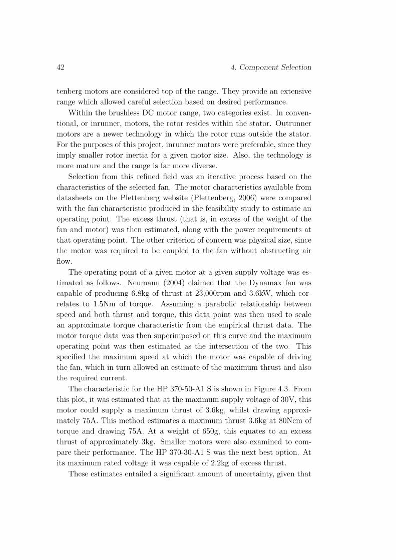
The characteristic for the HP 370-50-A1 S is shown in Figure 4.3. Fromthis plot, it was estimated that at the maximum supply voltage of 30V, thismotor could supply a maximum thrust of 3.6kg, whilst drawing approxi-mately 75A. This method estimates a maximum thrust 3.6kg at 80Ncm oftorque and drawing 75A. At a weight of 650g, this equates to an excessthrust of approximately 3kg. Smaller motors were also examined to com-pare their performance. The HP 370-30-A1 S was the next best option. Atits maximum rated voltage it was capable of 2.2kg of excess thrust.
These estimates entailed a significant amount of uncertainty, given that
4.1. Propulsion System 43
Figure 4.3: Plot of torque estimation for the 370-50-A1-S motor
the fan thrust-speed characteristic was extrapolated from low speeds. Giventhis uncertainty, the option with the largest excess thrust was selected,that is, the HP 370-50-A1 S. This motor is capable of drawing 90A atmaximum torque, whilst the design operating point is 75A, which allowedfor an overestimation of fan efficiency. It is equipped with a kevlar armouredrotor to allow high speed operation.
This thrust estimate was then used to determine a mass budget to mod-erate the remainder of the design. A thrust to weight ratio of 1.5 wasselected as a target to provide an adequate margin for error, which dictateda mass budget of 2.4kg.
4.1.3 Electronic Speed ControllerThe selection of an appropriate electronic speed controller is critical for thesafe and correct operation of a brushless DC motor. For brushless motorsthe ESC is responsible not only for regulating the supply voltage to themotor but also for performing the switching required for commutation. TheESC must not only be rated to the appropriate current and voltage, it mustalso be capable of the switching frequencies required. The commutationmechanism must also be suitable for the target motor. Poor selection cancause damage to both components.
44 4. Component Selection
Three options emerged that were suitable for the selected motor. At thelower end of the market, Hyperion produces a controller that is rated to42 volts and 90 amps, at a price of $315. It is not recommended, however,to run this current for extended periods. The Castle Creations Phoenix110-HV is rated to 50V and 110A, but it is more expensive at $370 andweighs 150g, see Figure 4.4. The selected motor is a ten pole motor, and itis required to operate above 20,000rpm. This speed controller is capable ofdriving a ten pole motor at 30,000rpm, so should be more than adequate.The motor is also equipped with a back emf sensing mechanism that ensurescorrect switching.
Figure 4.4: Photograph of Castle Creations Phoenix 110-HV (Castle Cre-ations, 2006)
Plettenberg recommended a larger chip, the Schulze Future 40-160H,which is rated to 40V and 160A. It is also capable of driving at 60,000rpmfor a four pole motor, which corresponds to 24,000rpm for a ten pole motor.The controller is considerably more expensive, at $630. It is also quite heavy,weighing 200g. It did not appear to have any distinct advantages over theCastle Creations controller. A smaller Schultze Future ESC, the 32-80Kmay be sufficient. It is rated to 32V and 95A, with the same speed limit.It is far lighter, at 60g, and less expensive, at $425. Plettenberg suggestedthat this controller may not sufficiently allow for surges in current.
The Castle Creations Phoenix HV-110 was selected as it satisfies speci-fication whilst providing significant savings in cost and weight.

4.1. Propulsion System 45
4.1.4 Power SupplyIn order to yield the optimum performance from the propulsion system,a power supply was desired that is capable of comfortably providing thedesign voltage and current was sought. This again afforded a margin oferror in mass budget and thrust estimates. Since the power supply is notonboard the vehicle, weight was not an important factor and selection wasbased on other criteria including:
• Charge capacity: The supply must be able to provide the requiredcurrent for a reasonable flight time.
• Variability of supply: As thrust generated varies with supply voltage,variations in the voltage will have a destabilising effect on the craft.The supply voltage should remain as constant as possible throughoutdischarge.
• Internal Resistance: At the high currents anticipated, the voltage dropdue to battery internal resistance is likely to be significant. It is soughtto be minimised.
4.1.4.1 Sealed Lead Acid (SLA) Batteries
Using 12V SLA batteries for the power source we would require 3 units inseries to satisfy our voltage requirements. In order to obtain a reasonableflight time it was calculated that we required a second bank of batteries inparallel for additional charge capacity.
The performance criteria discussed varied with the quality and price ofbattery, batteries ranging from less than one hundred to six hundred dollarswere considered.
Through liaison with premium supplier Battery Specialties, several bat-teries were found that would be capable of providing the stable outputvoltage required at an adequate charge capacity. For estimated power re-quirements of 30V and 75A:
• Using Sunlyte batteries of charge capacity 100Ah with 3 units in seriesand 2 in parallel (6 batteries in total)
• Operating @ 35A current draw each

46 4. Component Selection
• Output voltage = 3×10.2V = 30.6V
• Discharge time = 2 hours
• Total Battery cost = 6×$290 = $1740
The calculations show that a network of these batteries would be capableof supplying the craft with the estimated power required to hover, with anacceptable flight time.
These batteries can be charged at a maximum of 30A, and such wouldrequire over two hours of charge time. To charge all the batteries simulta-neously would require the purchase of six chargers, with the associated cost.The units also experience a voltage drop as they discharge, which meansthat the usable life of the battery could be even shorter than the quotedtwo hours.
4.1.4.2 Regulated DC Power Supplies
The Densei-Lambda units utilise mains power to generate a high power DCsource. The supply is regulated to ensure a constant voltage. The flight timeis not limited by the power supply nor is downtime for charging required.The only disadvantage to this option is the cost. Care must also be takento protect load components.
Whilst they are more expensive, the regulated supplies are a more valu-able asset for the School than a large amount of SLA batteries. The purchaseof two 40V-38A Densei-Lambda units (Figure 4.5) was approved. The sup-plies can be connected in parallel to produce the current required by thecraft.
Figure 4.5: Photograph of the Densei-Lambda power supplies selected

4.2. Control Hardware System 47
4.2 Control Hardware SystemThe control hardware system comprises the actuators, sensors and signalinterfacing hardware required to control the craft. Careful selection of thesecomponents was required to provide the control hardware system with thecapacity to achieve stable hover.
4.2.1 Servo Motors
Servo performance is critical to the success of such vehicles, so the selec-tion of servos required some thought. As discussesd by Fleming and Jones(2003), the disturbance rejection capacity of the system is essentially a func-tion of maximum pitch and roll rates, which are limited by servo bandwidth.This is particularly the case for small scale light weight vehicles with smallinertias (Avanzini and Matteis, 2006).
Also, torque capacity requires consideration, light weight is desirable andexcessive mechanical free-play and electrical dead-band should be avoided(Lipera et al., 2001). This dead-band is defined by Futaba (2006) as theangles around the centre of travel where there is sluggish or no response.Since the servos are required to operate with fine angular resolution aroundthe centre of travel, this is highly undesirable.
Servo motor manufacturers do not publish frequency response informa-tion in the data sheets and hence testing was necessary to obtain this. Theprocess of selecting an appropriate servo was therefore based on the resultsof the testing as well as research done into the workings of the servo motor.
4.2.1.1 Background on Servo Motors
Servo motors are composed of a DC motor, an amplifier that receives thePWM signal and applies power to the motor coils, and the gear train whichtransmits the power to the output shaft. For the purposes of justifying thedecisions made a brief discussion of each component follows.
DC motor This is either a standard iron core brushed DC motor or acoreless variety. The coreless variety simply has the coils fastened into shapewith glue, and has the advantage of a greatly reduced rotor inertia (Hitec,2006).

48 4. Component Selection
Gear train The material that the gears are fabricated from has an im-portant influence on its performance. In ascending order of toughness thematerials used are Nylon, Karbonite, Metallic alloy and Titanium.
Karbonite gears are a new innovation and compose of dense plastic whichmakes them approximately six times stronger than the standard nylon gears.The Karbonite gear train allows superior resolution and does not suffer fromthe backlash problems present in metallic alloy gear trains after wear.
Titanium gears exhibit negligible wear and have superior strength, mak-ing them suitable for high torque applications.
Amplifier Until recently, servo motors have exclusively used analoguecomponents to amplify the PWM control signal. Servo motors contain adigital amplifier have recently entered the market and are commonly referredto as “digital servos”.
Digital servos provide advantages over their analogue counterparts interms of dead-band reduction, response time and resolution, making theman attractive option. Figure 4.6 demonstrates the benefits in servo response.
Deadband reduction is achieved because digital units no longer havethe significant dead time that the slower switching analogue models possess(Futaba, 2006). The faster pulses are able to deliver power more fluentlyand allow control of smaller, more precise movements, see Figure 4.7.
Figure 4.7 illustrates how the digital amplifier updates the command tothe motor at 300Hz instead of the 50Hz used in their analogue counterparts.This allows both the improved torque response shown in Figure 4.6 and theimproved resistance to load fluctuations. Since it is updated much quickerthe servo has an increased ability to hold a given position.
The advantages of digital servo motors are particularly relevant to theproject specifications. It was decided to purchase a digital servo motor totest and compare to other servo motors used on previous projects.
4.2.1.2 Estimated Torque Requirements
The calculations of Appendix D.1 gave an upper limit on the aerodynamicforces. From this the minimum torque capabilities of the servo were deter-mined. Figure 4.8 illustrates the critical locations for a vane cross-section.
The analysis is conservative in the distance between the shaft axis andcentre of pressure and also in the applied force. Based on these calculations,

4.2. Control Hardware System 49
Figure 4.6: Illustration of the improved response of digital servos (Futaba,2006)
S9450 - Digital servo, S9402 - Analogue servo
Figure 4.7: Diagram showing increased signal frequency of digital servos(Futaba, 2006)

50 4. Component Selection
Figure 4.8: Diagram of the critical vane locationswhereL = Control vane length = 0.1mFmax = Maximum control vane force = 1NTmax = Maximum torque imposed on the servo = FmaxL
2= 0.05Nm
the torque requirements will be easily met by small commercially availableservos.
4.2.1.3 Servo Frequency Response Testing
The setup for the testing the frequency response was as follows. A poten-tiometer was mounted to the servo output shaft and the servo excited with achirp input as shown in Figure 4.9, the response was obtained by measuringthe voltage across the potentiometer. The transfer function and bandwidthof the servo motor can then be determined from a Fourier transform of theinput and output data. Figure 4.10 outlines the set up configuration.
The range of interest was 0–10 Hz, so the input range over this span in100 seconds.
Figure 4.9: Diagram of a chirp wave form and output oscillating shaft dis-placement

4.2. Control Hardware System 51
Figure 4.10: Schematic of servo testing rig
The testing rig was created by modifying the breakout board used inthe fan testing. Serial port pins are used to interface the input and outputBNC leads from the dSPACE board. The PWM signal driving the servomotor was interfaced to its control pin, the output of the pot was fed todSPACE through serial pins. Power was supplied to both of the units froma 7.4V LiPo battery.
The first stage in this process was to test the following three servo motorsowned by the department.
• JR577
• JR579
• Epsilon ε381
These servo motors all contained iron core motors and analogue amplifiers.The JR577 and ε381 servo contained nylon gears and the JR579 containedmetallic gears.
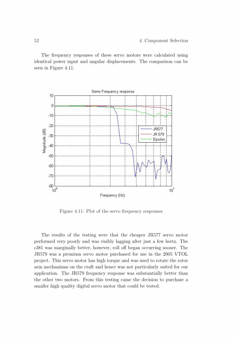
52 4. Component Selection
The frequency responses of these servo motors were calculated usingidentical power input and angular displacements. The comparison can beseen in Figure 4.11.
Figure 4.11: Plot of the servo frequency responses
The results of the testing were that the cheaper JR577 servo motorperformed very poorly and was visibly lagging after just a few hertz. Theε381 was marginally better, however, roll off began occurring sooner. TheJR579 was a premium servo motor purchased for use in the 2005 VTOLproject. This servo motor has high torque and was used to rotate the rotorarm mechanisms on the craft and hence was not particularly suited for ourapplication. The JR579 frequency response was substantially better thanthe other two motors. From this testing came the decision to purchase asmaller high quality digital servo motor that could be tested.
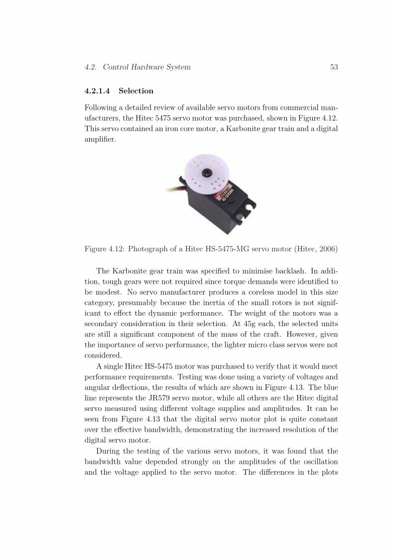
4.2. Control Hardware System 53
4.2.1.4 Selection
Following a detailed review of available servo motors from commercial man-ufacturers, the Hitec 5475 servo motor was purchased, shown in Figure 4.12.This servo contained an iron core motor, a Karbonite gear train and a digitalamplifier.
Figure 4.12: Photograph of a Hitec HS-5475-MG servo motor (Hitec, 2006)
The Karbonite gear train was specified to minimise backlash. In addi-tion, tough gears were not required since torque demands were identified tobe modest. No servo manufacturer produces a coreless model in this sizecategory, presumably because the inertia of the small rotors is not signif-icant to effect the dynamic performance. The weight of the motors was asecondary consideration in their selection. At 45g each, the selected unitsare still a significant component of the mass of the craft. However, giventhe importance of servo performance, the lighter micro class servos were notconsidered.
A single Hitec HS-5475 motor was purchased to verify that it would meetperformance requirements. Testing was done using a variety of voltages andangular deflections, the results of which are shown in Figure 4.13. The blueline represents the JR579 servo motor, while all others are the Hitec digitalservo measured using different voltage supplies and amplitudes. It can beseen from Figure 4.13 that the digital servo motor plot is quite constantover the effective bandwidth, demonstrating the increased resolution of thedigital servo motor.
During the testing of the various servo motors, it was found that thebandwidth value depended strongly on the amplitudes of the oscillationand the voltage applied to the servo motor. The differences in the plots

54 4. Component Selection
Figure 4.13: Plot of the HS-5475 response compared to analogue servomotors

4.2. Control Hardware System 55
in Figure 4.13 highlights the importance of matching the conditions of thetesting to those experienced on the craft. Following the methodology of theCarlsson and Cronander paper (2004), small angular deflections were usedto model the high frequency, low amplitude adjustments that best reflectthe demands of the control system. If larger angular movements were used,the response would effectively be limited by the slew rate (or maximumspeed) of the motor. The motors were also tested with the inertial loadingof the vanes present which caused a slight reduction in amplitude at higherfrequencies.
Two different batteries were used for the testing. A 7.4V LiPo batteryand a 4.8V NiCad cell. It was noticed that the signal contained much morenoise when the 7.4V battery was used, indicating that the higher voltagecaused problems with the motor controller leading to overshoot in the re-sponse. For this reason, a voltage regulator was installed on the PicoPicservo controller such that the voltage supplied to the servo motors was 6V,compromising between the speed of the servo while removing the excessnoise from the internal potentiometer and hence removing the jittering thatwas present.
Based on the testing results the Hitec digital servos were found to ade-quately satisfy the performance requirements outlined. Three further mo-tors were then purchased. Discussion of the modelling of these servo motorsis included in Chapter 7.
4.2.2 Servo Motor Battery
The servo motors require an independent voltage in the order of 6 Volts.The current requirements are minimal. Given this, it was possible to powerthe servos from a single onboard Lithium Polymer (LiPo) source. The2005 VTOL project powered servos from a 7.4V LiPo that weighed 80g.If necessary, servo power can also be provided via a tether, though thereduction in mass is minimal and the addition to tether size is undesirable.
LiPo batteries are the newest battery cell technology and the mostfavourable in terms of charge capacity to weight. The cells are availablein 3.7V increments, hence the 7.4V cell would be the most appropriate.The existing LiPo is suitable and is shown in Figure 4.14.

56 4. Component Selection
Figure 4.14: Photograph of the servo motor battery
4.2.3 Sensors
The department owns two sensors, both of which were evaluated for usein this project. They differ greatly in function and also in their limita-tions. The options available were to use either sensor independently, oralternatively both could be used for measurement of different states. Thecapabilities of the sensors are outlined as follows.
Logitech Head Tracker Ultrasonic Sensor This sensor is capable ofproviding position information for all translational and rotational degreesof freedom (6 DOF). The fixed transmitter sends ultrasonic pulses to thereceiver and using time delay information, the control unit can deduce theposition and angle of the receiver. The sensor measures absolute positionand angle, and would need to be differentiated to provide angular rates.
The active area is limited to a 100 degree spherical cone, that extendsfrom the transmitter for 5 feet. This spatial limitation would restrict anymovement of the platform other than vertical hover. The operating rangeis shown in Figure 4.15.
The main advantage of this sensor from a control perspective is theexceptional accuracy. The translational resolution is quoted as one 250th ofan inch (about 0.1mm) and rotational resolution for pitch, roll and yaw isone tenth of a degree. These states are all updated at 50Hz (sample every20ms) with a 30ms processing latency making it relatively fast as comparedto other elements in the control loop. This processing latency may causeissues with closed loop stability, which will require attention at a later date.
The limitation of the ultrasonic signal is its sensitivity to air flow distur-

4.2. Control Hardware System 57
Figure 4.15: Diagram of the Logitech Head Tracker sensor showing workingrange (Depo, 2006)
bances and acoustic noise. It was experimentally verified that the consid-erable air pressure fluctuations present around the craft would induce noisein the signal, reducing the accuracy of the measurements.
Since the sensor uses ultrasonics, it requires direct line of sight to theground receiver. Ideally, for simplicity, it should be placed at the centralaxis of the craft, but care must be taken to avoid obstruction of the air flowthrough the duct. The flow may also cause excessive noise in the sensorsignal, which must also be avoided.
If the receiver moves out of range or out of sight, the program will setthe “out of range” bit on the control unit. When this bit is set the outputis not measured but instead the last valid data point is stored. The controlsystem will need to closely monitor position and speed to prevent this fromoccurring, since it will effectively open the control loop. These issues canbe overcome, and given that the vehicle is to be tethered, they will need tobe overcome regardless of the sensor used.
MicroStrain 3DM-GX1 This sensor is a high end Inertial MeasurementUnit (IMU) with internal signal processing and filtering capabilities. It waspurchased in 2005 for use in the VTOL project. The unit contains:
• Three angular rate gyroscopes

58 4. Component Selection
• Three orthogonal DC accelerometers
• Three orthogonal magnetometers
• A multiplexer
• A 12 bit analogue-to-digital converter
• An embedded microcontroller
The sensor has been proven to provide reliable measurement of angles andangular rates, however the measurement of absolute position with such asensor is problematic. Double integration of data from the accelerometersis required to obtain position information. This means that any offset inthe accelerometer will result in a quadratic change in the position stateafter double integration. Thus the measurement of position in this man-ner inherently contains these errors that are of a non-zero mean and thedrift continues to accumulate, making the estimate of the craft positionprogressively worse.
For this reason, the 3DM-GX1 (see Figure 4.16) is suitable for stabilisingthe craft in an angular rate-based controller, provided that some form ofdrift correction is integrated.
Figure 4.16: Photograph of the MicroStrain 3DM-GX1 (Microstrain, 2006)
Sensor Strategy The gyroscopic coupling between the pitch and roll axesis manifest in a moment that is proportional to angular rates. Consequently,an accurate estimate of these rates is required to effective compensate for

4.2. Control Hardware System 59
this coupling. Differentiation would be necessary to obtain rates from theLogitech sensor, and the disturbance from acoustic noise would make thisparticularly unreliable. The IMU is capable of providing far more accuraterate data, and as such, it was decided to implement this sensor in a rate-based system.
Two methods are available to correct drift in rate-based systems. Thefirst is “pilot in the loop” control whereby a human operator regulates po-sition by means of an input device such as a joystick. The alternative is tointegrate a second sensor in a Kalman filtering arrangement. This methodis used by a number of military UAV platforms to integrate IMU and GPSdata (Lipera et al., 2001). This allows the inertial unit to regulate the sta-bility of the craft, while the GPS periodically corrects for drift in absoluteposition estimates. In the context of this project, the Logitech sensor mayprovide drift correction for the rate-based system by the same method. Thisconfiguration is necessary to achieve autonomous 6 DOF regulation.
4.2.4 Signal Interfacing Hardware
Control of the craft requires that sensors and actuators be interfaced suc-cessfully to allow feedback regulation. This can be done on a microcontrollerfor onboard control, however since the craft was operating with a tether,static hardware was used for its ease of implementation and adaptability.Thus the incoming sensor data and outgoing control signals are sent via thecraft tether.
4.2.4.1 dSPACE Platform
The dSPACE control platform, shown in Figure 4.17 contains A/D con-verters, encoders, four PWM outputs, a serial port and a Digital SignalProcessor (DSP) to process the signals and execute control loops.
Models designed in Simulink are compiled to “C” and downloaded tothe board for execution by the DSP. A Simulink toolbox provides refer-ences for the ports of the dSPACE board that allows integration in theSimulink model. The “DS1104” blocks in the example Simulink modelin Figure 4.18, refer to input/output ports of the platform.
The dSPACE platform has its own graphical user interface softwarecalled ControlDesk which can display and log the values of parameters
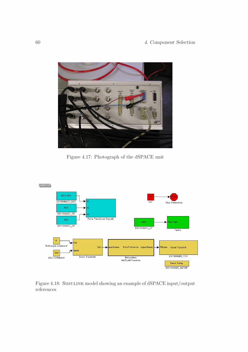
60 4. Component Selection
Figure 4.17: Photograph of the dSPACE unit
Figure 4.18: Simulink model showing an example of dSPACE input/outputreferences

4.2. Control Hardware System 61
while allowing real time model manipulation. A typical graphical output isshown in the Figure 4.19.
Figure 4.19: ControlDesk graphical output example
4.2.4.2 PicoPic Microcontroller
The dSPACE platform contained four PWM output channels, however, tocontrol the main DC motor and four servo motors, five PWM signals werenecessary. The PicoPic microcontroller as shown in Figure 4.20 was in-terfaced through the serial port of the dSPACE board and generated therequired PWM signals.
The PicoPic was modified such that a single power supply could be usedfor the board logic and for the servo motors. This was necessary becausethe servo motors required six volts for optimal performance and 5V ± 5%was needed to run the microcontroller. Using a single battery resulted ina significant saving in weight and allowed fast transit time for the servomotors.
The serial port was detached to save space, with the receive and groundpins soldered onto the board. Since data is not sent from the PicoPic, thetransmit pin was not required.
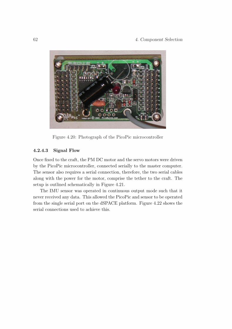
62 4. Component Selection
Figure 4.20: Photograph of the PicoPic microcontroller
4.2.4.3 Signal Flow
Once fixed to the craft, the PM DC motor and the servo motors were drivenby the PicoPic microcontroller, connected serially to the master computer.The sensor also requires a serial connection, therefore, the two serial cablesalong with the power for the motor, comprise the tether to the craft. Thesetup is outlined schematically in Figure 4.21.
The IMU sensor was operated in continuous output mode such that itnever received any data. This allowed the PicoPic and sensor to be operatedfrom the single serial port on the dSPACE platform. Figure 4.22 shows theserial connections used to achieve this.
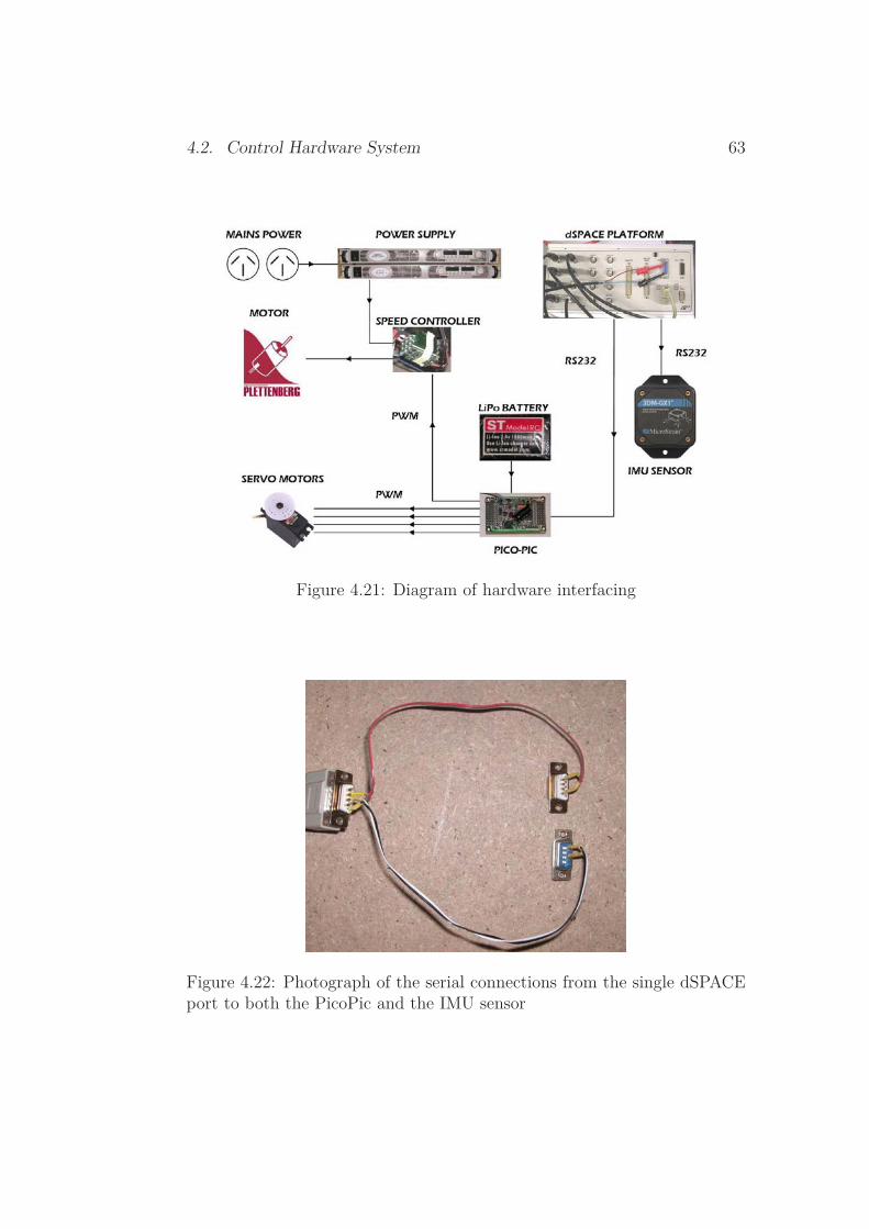
4.2. Control Hardware System 63
Figure 4.21: Diagram of hardware interfacing
Figure 4.22: Photograph of the serial connections from the single dSPACEport to both the PicoPic and the IMU sensor


Chapter 5
Dynamics & Modelling
The dynamics of a design concept form the basis upon which a controlsystem is built. Consideration of dynamic behaviour in mechanical designcan vastly simplify the task of controller development. The first section ofthis chapter provides a qualitative discussion of the dynamic considerationsthat shaped the criteria for mechanical design. In the second section, thelinearised mathematical model of the craft dynamics is derived.
5.1 Vehicle Dynamics, Stability and Control-lability
Good aircraft design is a compromise between stability and controllability,as the two are inversely related. Designing for these considerations is a diffi-cult process that depends on many variables. Parameters such as placementof the vehicle’s centre of gravity, placement of actuators, and moments ofinertia about each axis of rotation largely determine the dynamic behaviourof the vehicle and its limitations. Since open loop and closed loop dynamicsare interrelated, careful mechanical design can greatly simplify developmentof the control system in the future.
As discussed in Section 6.3.3, control vanes are limited in that they areboth non-linear and saturate by stall at excessive angles of attack. Thecoupling between yaw and pitch/roll results in compounded control vanedeflection when yaw and pitch/roll control demands coincide. Capacity forboth disturbance rejection and command following is required. To mitigatethese issues as much as possible, vehicle centre of gravity and control vane
65
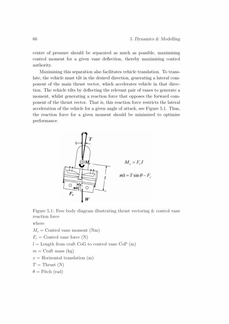
66 5. Dynamics & Modelling
centre of pressure should be separated as much as possible, maximisingcontrol moment for a given vane deflection, thereby maximising controlauthority.
Maximising this separation also facilitates vehicle translation. To trans-late, the vehicle must tilt in the desired direction, generating a lateral com-ponent of the main thrust vector, which accelerates vehicle in that direc-tion. The vehicle tilts by deflecting the relevant pair of vanes to generate amoment, whilst generating a reaction force that opposes the forward com-ponent of the thrust vector. That is, this reaction force restricts the lateralacceleration of the vehicle for a given angle of attack, see Figure 5.1. Thus,the reaction force for a given moment should be minimised to optimiseperformance.
Figure 5.1: Free body diagram illustrating thrust vectoring & control vanereaction forcewhereMc = Control vane moment (Nm)Fc = Control vane force (N)l = Length from craft CoG to control vane CoP (m)m = Craft mass (kg)x = Horizontal translation (m)T = Thrust (N)θ = Pitch (rad)

5.1. Vehicle Dynamics, Stability and Controllability 67
This requirement raises the question of motor-fan configuration. Ifthe motor is mounted below the fan, as the Dynamax fan design intends,the centre of gravity is inevitably located below the thrust vector. Thispendulum-like configuration (Figure 5.2) has inherent stability (Schlecht,2000), which is optimised by a low centre of gravity. This detracts fromseparation of centre of gravity and control vanes, reducing control authority.Increasing the length of the duct is not desirable, as it allows for increasedflow losses and disturbances in the flow field (Fleming and Jones, 2003).
Figure 5.2: Diagram of different motor/fan configurations
An alternative configuration, which has been used in many designs in-cluding the Micro Craft iStar (Lipera et al., 2001) and the AROD (Whiteand Phelan, 1991), sees the motor mounted above the fan. This solutionprovides both a high centre of gravity and small control vane/fan separa-tion, but it also raises the question of stability. The problem now resemblesthe inverted pendulum, which is inherently unstable in open loop. To bestapproach this problem, the centre of gravity should be placed as high aspossible, to slow down the unstable pole as much as possible, to cater forclosed loop stability.
This second configuration appears to be the better of the two. Stabil-ity may not pose a big problem in closed loop. For Lipera et al. (2001),even with a top mounted drive the vehicle dynamics were characterised bytendency of the vehicle to return to stable hover. From a practical perspec-tive, designing a top-mounted drive for the Dynamax fan provides quite achallenge.
The question of stability depends a great deal on vehicle and actuator
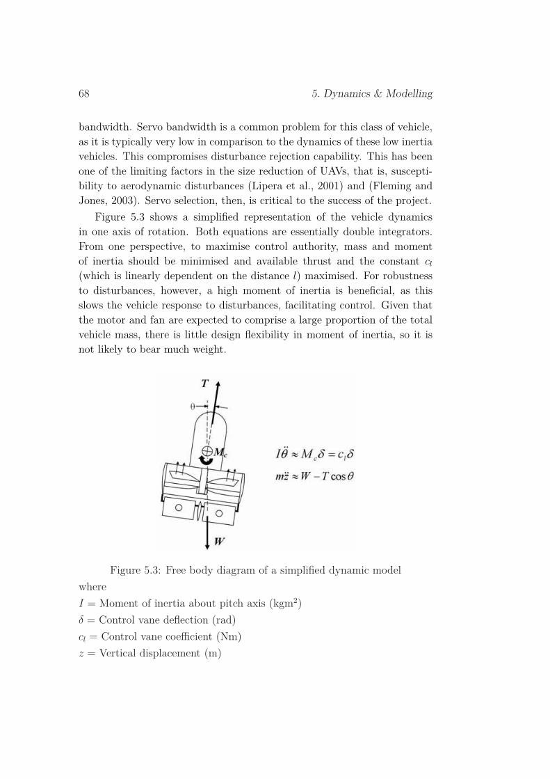
68 5. Dynamics & Modelling
bandwidth. Servo bandwidth is a common problem for this class of vehicle,as it is typically very low in comparison to the dynamics of these low inertiavehicles. This compromises disturbance rejection capability. This has beenone of the limiting factors in the size reduction of UAVs, that is, suscepti-bility to aerodynamic disturbances (Lipera et al., 2001) and (Fleming andJones, 2003). Servo selection, then, is critical to the success of the project.
Figure 5.3 shows a simplified representation of the vehicle dynamicsin one axis of rotation. Both equations are essentially double integrators.From one perspective, to maximise control authority, mass and momentof inertia should be minimised and available thrust and the constant cl
(which is linearly dependent on the distance l) maximised. For robustnessto disturbances, however, a high moment of inertia is beneficial, as thisslows the vehicle response to disturbances, facilitating control. Given thatthe motor and fan are expected to comprise a large proportion of the totalvehicle mass, there is little design flexibility in moment of inertia, so it isnot likely to bear much weight.
Figure 5.3: Free body diagram of a simplified dynamic modelwhereI = Moment of inertia about pitch axis (kgm2)δ = Control vane deflection (rad)cl = Control vane coefficient (Nm)z = Vertical displacement (m)

5.2. Mathematical Model 69
The aforementioned considerations assume only small perturbations aboutstable hover and ignore the effects of gyroscopic coupling. It is interesting tonote that angular momentum is exploited by Lim et al. (2004) to increasethe stability of their vehicle. This vehicle incorporates a rotating inertiawheel to generate an angular momentum vector in z-axis direction, therebyincreasing attitude stability. This may perhaps prove a positive implicationof the single drive concept, that is, the rotor inertia may act to stabilise thevehicle in hover.
This issue of vehicle dynamics, stability and controllability is obviouslyan intricate one. Given the stability issues inherent in this class of vehi-cle, stable hover should be the primary objective for vehicle design. Sincemany of the design considerations are conflicting and difficult to approachanalytically, extensive testing will be required to tune the system. Dueto the criticality of duct length and control vane placement, the vehiclewill initially utilise a variable length duct which will allow optimisation ofthese parameters by testing. These concepts were developed by personalcorrespondence with Wood (2006).
5.2 Mathematical ModelFor the purposes of control development, a mathematical model of the ve-hicle dynamics is required. Figure 5.4 shows a SolidEdge model of thecraft with co-ordinate axes.
The translational and rotational co-ordinates are defined in Equations 5.1and 5.2.
(θ, φ, ψ) = (pitch, roll, yaw) (5.1)
(x, y, z) = (x,y,z translations) (5.2)
The approach used to develop this model is presented by Castillo (2004).Figure 5.5 shows the free body diagram of the vehicle in pitch and roll.
5.2.1 Force BalanceThe summation of forces in the x, y and z coordinates is shown in Equa-tions 5.3, 5.4 and 5.5. The forces modelled include the thrust vector compo-nents, which are proportional to the square of rotor speed, and the controlvane reaction forces, which are approximated as proportional to angular

70 5. Dynamics & Modelling
Figure 5.4: SolidEdge model of the craft with co-ordinate axes
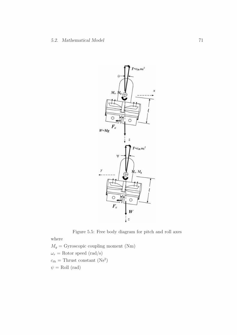
5.2. Mathematical Model 71
Figure 5.5: Free body diagram for pitch and roll axeswhereMg = Gyroscopic coupling moment (Nm)ωr = Rotor speed (rad/s)cth = Thrust constant (Ns2)ψ = Roll (rad)

72 5. Dynamics & Modelling
deflection (White and Phelan, 1991). This approximation holds for smallangles. Control vane deflection uses the same sign convention as the axesabout which the rotate (that is, the pitch and roll axes, see Section 5.2).The weight of the vehicle is also included.
Summation of Forces∑Fx = M
..x = cth sin(φ) cos(θ)ω2
r + cf (δleft + δright) (5.3)∑Fy = M
..y = cth cos(φ) sin(θ)ω2
r + cf (δfront + δback) (5.4)∑Fz = M
..z = −cth cos(φ) cos(θ)ω2
r + Mg (5.5)
whereM = Craft mass (kg)cth = Thrust constant (Ns2/rad2)cf = Force constant from vane deflection (N/rad)ωr = Rotor speed (rad/s)δ = Control vane deflection of the left, right, front and back control
vanes (rad)g = Gravitational constant (m/s2)
5.2.2 Moment Balance
The summation of moments about the pitch, roll and yaw coordinate axesis shown in Equations 5.6, 5.7 and 5.8. The moments modelled include thegyroscopic coupling moments, which is the product of rotor angular mo-mentum and the rate of change of the coupled angle, the reactive torqueproduced by rotor, which is proportional to the square of rotor speed, andcontrol vane moments.
Summation of Moments∑Mθ = Jyy
..
θ = −JRωr
.
φ + cm (δleft + δright) (5.6)∑Mφ = Jxx
..
φ = −JRωr
.
θ + cm (δfront + δback) (5.7)∑Mψ = Jzzψ = ctω
2r + cm (δleft − δright − δfront + δback) (5.8)
5.2. Mathematical Model 73
whereJyy, Jxx, Jzz = Moment of inertia of entire plant (including rotor) about
the pitch, roll and yaw axis (kgm2)JR = Moment of inertia of the rotor (kgm2)cm = Moment constant from vane deflection (Nm/rad)ct = Torque constant (Ns2/rad2)
5.2.3 State ModelThe following State Space Model of the craft dynamics have been formu-lated from the force and moment balance equations in previous sections.Cazzolato (2006), has formalised these equations for use in a state spacemodel, incorporating pitch, roll, yaw, height (z), servo actuator and rotorspeed dynamics. The following sections outline the dynamic equations usedin the model, the model itself is developed in Section .
5.2.3.1 State Variables
The state variables utilised in the model are the following:θ = Pitch angle (rad)φ = Roll angle (rad)ψ = Yaw angle (rad)z = Vertical displacement (m)
5.2.3.2 Plant Inputs
The servo inputs to the plant are the following:δθ = Pitch servo deflection angle (rad)δφ = Roll servo deflection angle (rad)δψ = Yaw servo deflection angle (rad)
It is also possible to control the primary thrust by spoiling. This involvesganging two pairs of adjacent vanes. By bringing them together the mainthrust is reduced. The servo input into the plant for the thrust spoil is:
δt = Thrust (spoil) servo setting (rad)
Note that when linearising the dynamics it has been assumed that the rotorspeed ΩR is constant,

74 5. Dynamics & Modelling
ΩR = ΩR, 0 (rad/s)
The actual inputs to the servos are:uθ = Desired pitch servo deflection angle (rad)uφ = Desired roll servo deflection angle (rad)uψ = Desired yaw servo deflection angle (rad)ut = Desired thrust (spoil) servo setting (rad)uΩ = Desired rotor speed setting (rad/s)
5.2.3.3 Pitch Dynamics
The pitch dynamics are governed by:
..
θ = Mθδθ − MR,θ
.
φ +.
φ.
ψ(Jzz − Jxx
Jyy
) ≈ Mθδθ + MR,φ
.
φ (5.9)
whereMθ = Tθ
Jyy= Pitch servo effectiveness in (1/s2)
Tθ = Fxlθ,φ = Pitch torque per unit angle in pitch servo (Nm)Fx = Force in the x - axis per unit angle in the pitch servo (N)lθ,φ = Control vane moment arm for pitch and roll (m)MR,θ =
JRΩR,0
Jxx= Pitch gyroscopic coupling coefficient (1/s)
Note the gryoscopic coupling between the pitch acceleration and roll rate.
5.2.3.4 Roll Dynamics
The roll dynamics are governed by:
..
φ = Mφδφ + MR,φ
.
θ +.
θ.
ψ(Jyy − Jzz
Jxx
) ≈ Mθδθ + MR,θ
.
ψ (5.10)
whereMφ =
Tφ
Jxx= Roll servo effectiveness in (1/s2)
Tφ = FyIθ,φ = Roll torque per unit angle in roll servo (Nm)Fy = Force in the y - axis per unit angle in the roll servo (N)MR,φ =
JRΩR,0
Jyy= Roll gyroscopic coupling coefficient (1/s)
Note the gryoscopic coupling between the roll acceleration and pitch rate.

5.2. Mathematical Model 75
5.2.3.5 Yaw Dynamics
The yaw dynamics are governed by:
..
ψ = Mψδψ − MY
.
ΩR +.
θ.
φ(Jyy − Jxx
Jzz
) = Mφδφ − MY
.
Ω (5.11)
whereMψ =
Tψ
Jzz= Yaw servo effectiveness in (1/s2)
Tψ = Yaw torque per unit angle in yaw servo (Nm)MY = JR
Jzz= Ratio of rotor inertia to body yaw inertia (1/s)
Note the input coupling between yaw acceleration and rotor speed.
5.2.3.6 Vertical Displacement Dynamics
The vertical displacement dynamics are given by:
..z = MT ∆ΩR − Mtδt (5.12)
whereMT = KT
M= Rotor thrust effectiveness (m/s)
KT = Thrust per unit rotor speed at hover (N/(rad/s))∆ΩR = ΩR − ΩR,0 = Change in rotor speed about hover (rad/s)Mt = Kt
M= Thrust (spoil) servo effectiveness (m/s2)
Kt = Thrust per unit angle in the spoil servo (N/rad)Note the lack of attitude coupling to thrust due to linearisation.
5.2.3.7 Servo Actuator Dynamics
The servo dynamics have been modelled as a second order system governedby the differential equation:
..
δi = −2ζiωi
.
δ − ω2i δi + ω2
i ui (5.13)
whereζi = Damping coefficient of the servo motorsωi = Natural frequency of the servo motor poles (rad/s)ui = Desired servo angle (rad)

76 5. Dynamics & Modelling
5.2.3.8 Rotor Speed Dynamics
Similarly we can model the rotor dynamics as a first order system governedby the differential equation:
.
ΩR = − 1
TΩ
ΩR +1
TΩ
uΩ (5.14)
whereTΩ = Time constant of the motor and speed controller (s)uΩ = Desired rotor speed (rad/s)
5.3 Virtual Reality (VR) ModelIn order to tune a PID or State Space Controller of the complex system dy-namics, a VR model of the craft was implemented. This allowed real-timevisualisation of the control effort on the system dynamics in the Simulinkenvironment. It also allows for the investigation of the coupled parame-ters governing the motion of the craft, such as gyroscopic coupling and yawrotation during start-up. From actually seeing how the craft responds toinputs such as step responses and disturbances, valuable insight to the im-plementation of the control and the effects on the mathematical dynamicscan be attained visually.
Generating the virtual reality model for use in Simulink was not atrivial task. The full assembly model of the craft, originally in Solid Edgewas broken into two categories: The main body (shell) and parts whichmove relative to the main body. Due to the functionality of the fan rotorand the four control vanes, they were saved separately. The shell of thecraft was then saved as an IGES file, then imported into 3D Studio Max5 and saved as a WRL file. The result is shown in Figure 5.6. The sameprocess was done for the fan rotor and a single control vane. These are alsoshown in Figure 5.6.
The resulting WRL files from 3D Studio Max 5 were then imported intoV-Realm Builder 2.0, which is the virtual reality package associated withMatlab and Simulink. All of the parts were imported and fitted in ahierarchical tree. This allowed the recognition of which parts move relativeto which bodies and which axes. For example, the fan rotor was importedas a child of the rotational dynamics (roll, pitch and yaw) and a child of the

5.3. Virtual Reality (VR) Model 77
Figure 5.6: 3D Studio Max 5 model of craft components

78 5. Dynamics & Modelling
shell. Rotational elements were introduced to define its location and axisof rotation, such that it was located along the y-axis and had the ability torotate about the y-axis alone. These definitions allowed the Simulink blockwithin the program to move accordingly when connected with the systemdynamics subsystem. The final model generated in V-Realm Builder 2.0 isshown in Figure 5.7.
Figure 5.7: V-Realm Builder 2.0 complete model
Upon completion of the model, a Simulink model was then created,which contained the system dynamics, controller and a generic VR block.The VR block was then linked to the V-Realm file and the desired axesof motion (such as rotation) were selected as inputs for the block (ie, theoutputs of the controller). This defined the motions which the craft and itschildren would undergo.

Chapter 6
Mechanical Design
In following from Chapter 5, the craft was to comprise a ducted fan drivenfrom above by a DC motor with servo-driven control vanes located in thefan efflux. The purpose of this phase of the project was therefore to designa structural system to achieve this. A considerable amount of thought andreiteration was required to produce a successful design.
6.1 Structural DesignThe structural design included the design of the following subsystems:
• Fan rotor system
• DC motor mount System
• Servo motor mounts
• Control vane couplings and bearings
• Ductwork
• Landing rig
Design criteria throughout all phases of the structural design included:
• Weight minimisation
• Minimisation of air flow restriction
79
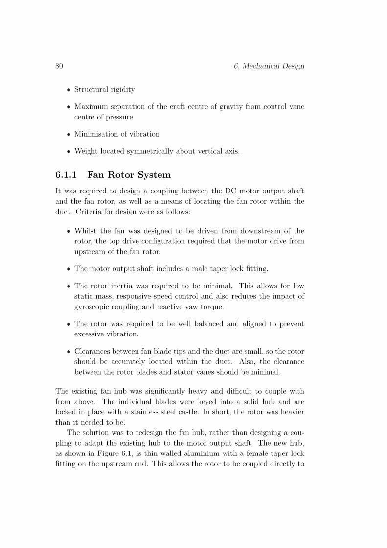
80 6. Mechanical Design
• Structural rigidity
• Maximum separation of the craft centre of gravity from control vanecentre of pressure
• Minimisation of vibration
• Weight located symmetrically about vertical axis.
6.1.1 Fan Rotor SystemIt was required to design a coupling between the DC motor output shaftand the fan rotor, as well as a means of locating the fan rotor within theduct. Criteria for design were as follows:
• Whilst the fan was designed to be driven from downstream of therotor, the top drive configuration required that the motor drive fromupstream of the fan rotor.
• The motor output shaft includes a male taper lock fitting.
• The rotor inertia was required to be minimal. This allows for lowstatic mass, responsive speed control and also reduces the impact ofgyroscopic coupling and reactive yaw torque.
• The rotor was required to be well balanced and aligned to preventexcessive vibration.
• Clearances between fan blade tips and the duct are small, so the rotorshould be accurately located within the duct. Also, the clearancebetween the rotor blades and stator vanes should be minimal.
The existing fan hub was significantly heavy and difficult to couple withfrom above. The individual blades were keyed into a solid hub and arelocked in place with a stainless steel castle. In short, the rotor was heavierthan it needed to be.
The solution was to redesign the fan hub, rather than designing a cou-pling to adapt the existing hub to the motor output shaft. The new hub,as shown in Figure 6.1, is thin walled aluminium with a female taper lockfitting on the upstream end. This allows the rotor to be coupled directly to
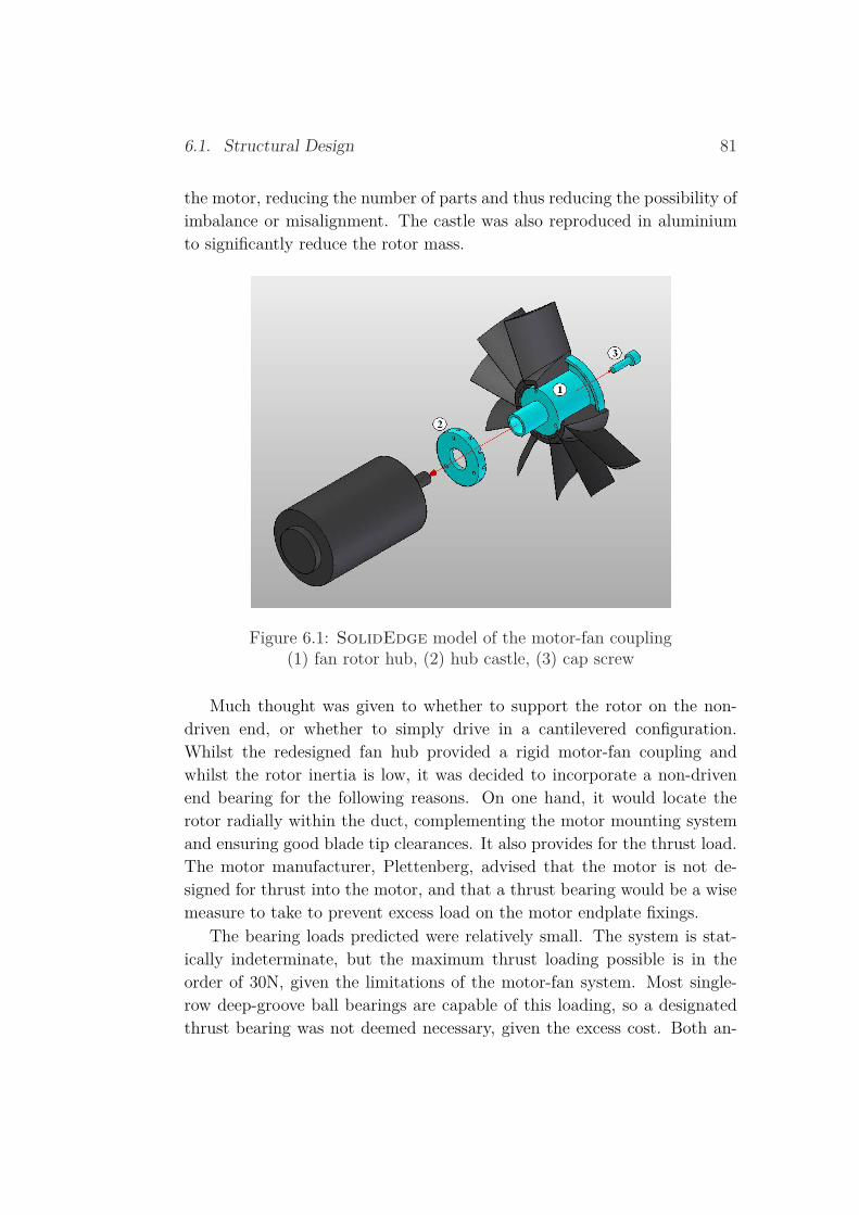
6.1. Structural Design 81
the motor, reducing the number of parts and thus reducing the possibility ofimbalance or misalignment. The castle was also reproduced in aluminiumto significantly reduce the rotor mass.
Figure 6.1: SolidEdge model of the motor-fan coupling(1) fan rotor hub, (2) hub castle, (3) cap screw
Much thought was given to whether to support the rotor on the non-driven end, or whether to simply drive in a cantilevered configuration.Whilst the redesigned fan hub provided a rigid motor-fan coupling andwhilst the rotor inertia is low, it was decided to incorporate a non-drivenend bearing for the following reasons. On one hand, it would locate therotor radially within the duct, complementing the motor mounting systemand ensuring good blade tip clearances. It also provides for the thrust load.The motor manufacturer, Plettenberg, advised that the motor is not de-signed for thrust into the motor, and that a thrust bearing would be a wisemeasure to take to prevent excess load on the motor endplate fixings.
The bearing loads predicted were relatively small. The system is stat-ically indeterminate, but the maximum thrust loading possible is in theorder of 30N, given the limitations of the motor-fan system. Most single-row deep-groove ball bearings are capable of this loading, so a designatedthrust bearing was not deemed necessary, given the excess cost. Both an-

82 6. Mechanical Design
gular contact ball bearings and needle roller bearings are significantly moreexpensive. The main selection criteria for bearing selection were speed rat-ing and mass. The bearing was required to be rated to at least 20,000rpm.Fortunately, smaller bearings are capable of higher speeds. A shielded bear-ing was selected to prevent the need for lubrication whilst allowing for thespeeds required. Specifications were sourced from the SKF online catalogue.
The bearing was incorporated into rotor in a system that maintains lowmass whilst preventing imbalance, as shown in Figure 6.2. It consists of adummy shaft and hub end cap that couple the fan rotor hub to the bearinginner race, as well as a thin-walled housing which locates the bearing outerrace within the fan stator. The end cap allows for both a hollow hub anda small diameter shaft. It is also stepped to prevent misalignment with thehub. The dummy shaft and housing are stepped to transmit thrust throughthe bearing to the fan stator. The housing has access holes to allow thehub to be disassembled from the bearing assembly. A cutaway view of theassembled rotor is shown in Figure 6.3.
Figure 6.2: SolidEdge model of the fan rotor bearing(1) nut, (2) hub end cap, (3) bearing housing,
(4) deep groove roller bearing, (5) dummy shaft

6.1. Structural Design 83
Figure 6.3: SolidEdge model of the fan rotor cutaway(1) hub castle, (2) hub, (3) hub end cap,
(4) dummy shaft, (5) bearing housing, (6) bearing
6.1.2 DC Motor Mount SystemIt was required to design a structural system to mount the motor to theexterior of the fan duct. Design criteria were as follows:
• The system was to facilitate and complement the rotor design de-scribed previously. That is, it was to mount the motor in the appro-priate axial and radial location as specified by the rotor design.
• The loads anticipated on the mounts were numerous. Firstly, themounts were required to stabilise the static weight of the motor. Sec-ondly, the thrust transmitted to the motor, which was statically in-determinate, and the reactive torque was required to be transmittedthrough the mounts to the fan duct. Finally, any vibration, both tor-sional due to cogging and radial due to any imbalance or misalignment,was required to be minimised.
• The system was required to be lightweight. It was also required topose minimal obstruction to the inlet airflow to the fan, since part ofthe structure was required to traverse this inlet.
• The provisions for mounting to the fan duct were minimal. The ductis made from a plastic of about 2mm wall thickness which was sus-
84 6. Mechanical Design
pected to be quite brittle. Any fixings were required to pose minimalobstruction to flow or rotating components within the duct.
The design solution consisted of aluminium brackets fixed to both the motorand the fan duct with struts of 4mm diameter carbon fibre rod. The systemconsists of two sets of four equi spaced struts, as shown in Figures 6.4 & 6.5.The top struts are located at the midpoint of the motor and are mountedit by means of a split circular clamp. These struts primarily provide staticstability to the motor. The bottom struts mounted to the motor by meansof a plate that utilises the bolt-hole pattern in the front-plate of the motor.These struts are tangential to the motor, thereby providing torsional stiff-ness under compression of the struts. This provides a much stiffer structurethan radial torsion members as the struts are far more rigid under compres-sion than bending. Given the magnitude of the reactive torque expected,that is, no more than one Nm, and their short length, there is no possibilityof these torsion members buckling.
Figure 6.4: SolidEdge model of the motor mounts (top view)(1) motor, (2) fan duct, (3) torsion strut, (4) top strut
This configuration of struts provides excellent rigidity under all loadsand modes of vibration. Any thrust transmitted to the motor is distributed

6.1. Structural Design 85
Figure 6.5: SolidEdge model of the motor mounts (side view)(1) motor clamp, (2) top struts, (3) torsion struts,
(4) motor front plate, (5) short duct bracket, (6) long duct bracket
between the struts. The overall mounting system of the motor-fan set isshown schematically in Figure 6.6. Evidently, the combination of bearingand struts provides not only for static loading but also for the modes ofvibration mentioned previously.
The struts are mounted to the fan duct by means of two pairs of alu-minium brackets, as shown in Figures 6.4 & 6.5. Each of the four bracketshas identical strut-hole patterns that co-locate one of each of the top andtorsion struts. One pair of struts is long, spanning the length of the fanduct. These long brackets make use of a pair of M3 bolt holes that span thefan duct through two long stator vanes. They also provide for two verticalcolumns that mount the servo assembly to the fan-motor assembly, as wellas provisions for mounting the device to a fixed six-axis force transducerfor testing. These functions will be discussed in a subsequent section. Thelong brackets are ribbed for weight reduction.
The short brackets provide the sole function of fixing the motor struts tothe fan duct. In order to make these brackets as light as possible, they wereto be fixed as close as possible to the duct lip. However, the fixings could

86 6. Mechanical Design
Figure 6.6: SolidEdge model of the motor-fan supports
not interfere with the fan rotor, which was within millimetres of the internalduct wall. The solution was to fix the brackets to the duct from within theduct with two M3 cap head screws countersunk into the duct wall. Thisallowed for the fixings to be flush with the duct wall whilst providing a rigidmount. This method was also used for the remaining two of three fixingsused for the long brackets.
Some thought was also given to the means of fixing the struts to thealuminium brackets. All the holes were specified as blind such that allcompression members are locked in place. The torsion members are locatedsuch that they are under compression loading due to the motor reactivetorque. As an additional measure, the struts were adhered in the holes withKwik Grip. This adhesive provides a soft elastic mount that will provide adegree of vibration damping and will not fracture under fatigue.
The structural integrity of this system was evident in the assembly pro-cess. The process evolved as follows. Firstly, the brackets were mountedto the fan duct, from which the stator vanes had been removed to facili-tate this. The stator vanes and central hub were then replaced, with thebearing assembly mounted within the hub. Next, the clamp and front-platewere fitted to the motor body and the fan rotor to the motor output shaft.
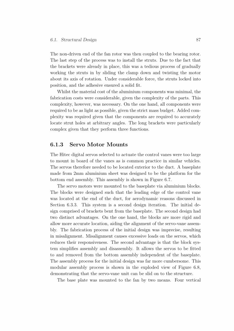
6.1. Structural Design 87
The non-driven end of the fan rotor was then coupled to the bearing rotor.The last step of the process was to install the struts. Due to the fact thatthe brackets were already in place, this was a tedious process of graduallyworking the struts in by sliding the clamp down and twisting the motorabout its axis of rotation. Under considerable force, the struts locked intoposition, and the adhesive ensured a solid fit.
Whilst the material cost of the aluminium components was minimal, thefabrication costs were considerable, given the complexity of the parts. Thiscomplexity, however, was necessary. On the one hand, all components wererequired to be as light as possible, given the strict mass budget. Added com-plexity was required given that the components are required to accuratelylocate strut holes at arbitrary angles. The long brackets were particularlycomplex given that they perform three functions.
6.1.3 Servo Motor Mounts
The Hitec digital servos selected to actuate the control vanes were too largeto mount in board of the vanes as is common practice in similar vehicles.The servos therefore needed to be located exterior to the duct. A baseplatemade from 2mm aluminium sheet was designed to be the platform for thebottom end assembly. This assembly is shown in Figure 6.7.
The servo motors were mounted to the baseplate via aluminium blocks.The blocks were designed such that the leading edge of the control vanewas located at the end of the duct, for aerodynamic reasons discussed inSection 6.3.3. This system is a second design iteration. The initial de-sign comprised of brackets bent from the baseplate. The second design hadtwo distinct advantages. On the one hand, the blocks are more rigid andallow more accurate location, aiding the alignment of the servo-vane assem-bly. The fabrication process of the initial design was imprecise, resultingin misalignment. Misalignment causes excessive loads on the servos, whichreduces their responsiveness. The second advantage is that the block sys-tem simplifies assembly and disassembly. It allows the servos to be fittedto and removed from the bottom assembly independent of the baseplate.The assembly process for the initial design was far more cumbersome. Thismodular assembly process is shown in the exploded view of Figure 6.8,demonstrating that the servo-vane unit can be slid on to the structure.
The base plate was mounted to the fan by two means. Four vertical
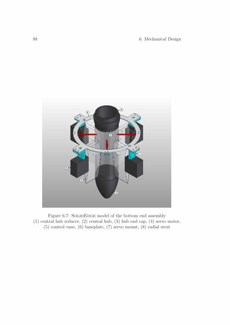
88 6. Mechanical Design
Figure 6.7: SolidEdge model of the bottom end assembly(1) central hub reducer, (2) central hub, (3) hub end cap, (4) servo motor,
(5) control vane, (6) baseplate, (7) servo mount, (8) radial strut
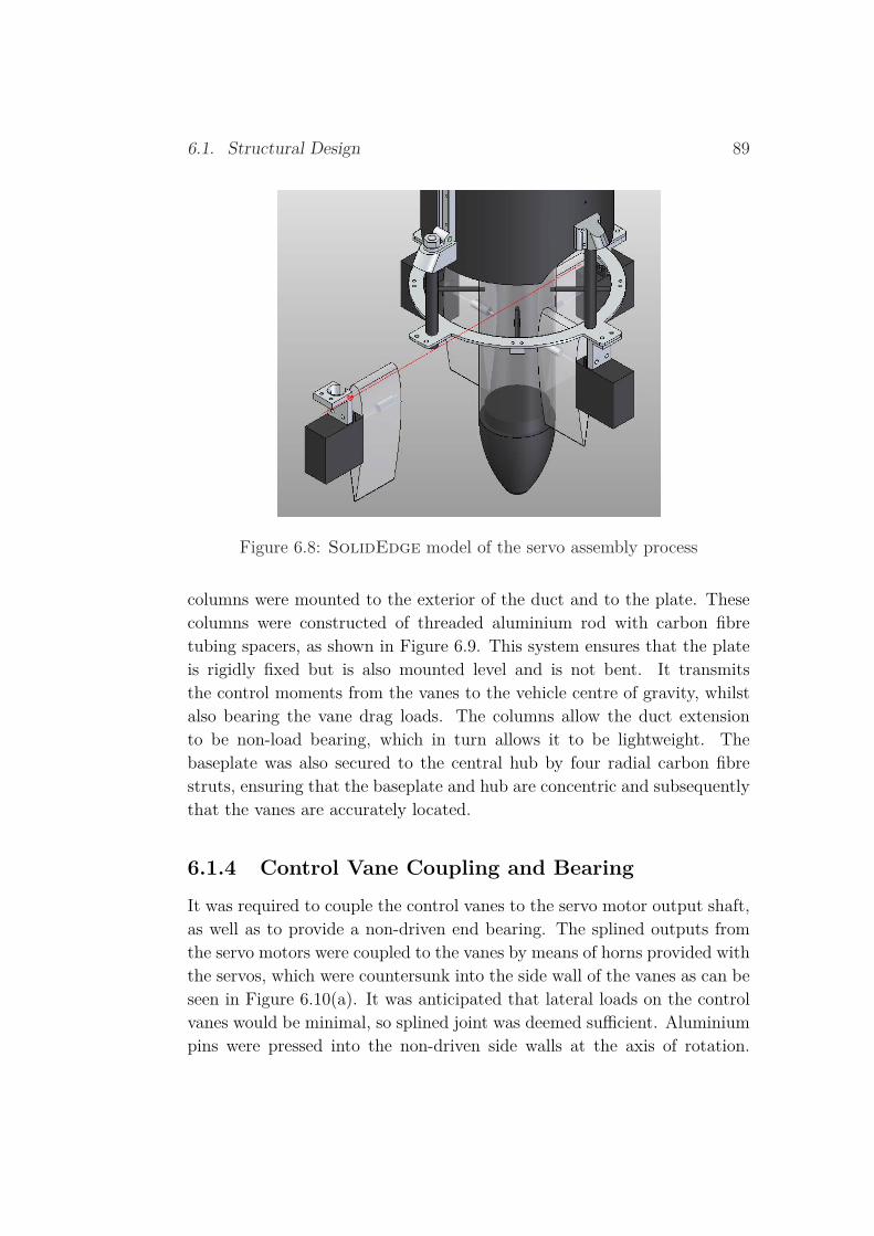
6.1. Structural Design 89
Figure 6.8: SolidEdge model of the servo assembly process
columns were mounted to the exterior of the duct and to the plate. Thesecolumns were constructed of threaded aluminium rod with carbon fibretubing spacers, as shown in Figure 6.9. This system ensures that the plateis rigidly fixed but is also mounted level and is not bent. It transmitsthe control moments from the vanes to the vehicle centre of gravity, whilstalso bearing the vane drag loads. The columns allow the duct extensionto be non-load bearing, which in turn allows it to be lightweight. Thebaseplate was also secured to the central hub by four radial carbon fibrestruts, ensuring that the baseplate and hub are concentric and subsequentlythat the vanes are accurately located.
6.1.4 Control Vane Coupling and Bearing
It was required to couple the control vanes to the servo motor output shaft,as well as to provide a non-driven end bearing. The splined outputs fromthe servo motors were coupled to the vanes by means of horns provided withthe servos, which were countersunk into the side wall of the vanes as can beseen in Figure 6.10(a). It was anticipated that lateral loads on the controlvanes would be minimal, so splined joint was deemed sufficient. Aluminiumpins were pressed into the non-driven side walls at the axis of rotation.

90 6. Mechanical Design
Figure 6.9: SolidEdge model of the vertical columns(1) fan duct, (2) duct bracket, (3) aluminium rod,
(4) carbon fibre spacer, (5) baseplate, (6) landing strut
6.1. Structural Design 91
These pins were to form dry rubbing bearings with the central hub, whichwas to be fabricated from a self-lubricating polymer. These bearings ensurethat the vanes maintain accurate alignment during operation, allowing fora tight clearance with the central hub. The vanes were hollowed out wherepossible for weight reduction, as shown in Figure 6.10(b).
(a) (b)
Figure 6.10: Photographs of the control vane fixings
6.1.5 DuctworkIn order to extend the annular flow section from the fan duct to the controlvanes, two components were required. The central hub previously referredto was required to extend the void section. A duct wall was also required tocontain the flow. The flow section essentially mimicked that of the fan efflux,for aerodynamic reasons which are discussed in Section 6.3.5. The length ofthe duct extension was designed with consideration of flow characteristics,vehicle dynamics and also component housing. The design rationale was asfollows.
6.1.5.1 Duct Length Optimisation
As discussed previously, the placement of the vanes with respect to vehiclecentre of gravity was thought to be critical to the actuator control authority

92 6. Mechanical Design
as well as the dynamic behaviour of the vehicle. The dynamic equations(6.1 & 6.2) of two degrees of freedom will demonstrate this.
ΣFx = m..x = cfδ + T sin θ (6.1)
ΣMy = Jyy
..
θ = cmlθ,φδ + (JRωr).
φ (6.2)
Whereby the notation utilised in these equations is taken from thatof Chapter 5. The dynamic equations demonstrate that for a given vanedeflection δ, control arm lθ,φ acts as a linear gain on the control momentgenerated. However, as control arm varies so does the vehicle moment ofinertia. Therefore, as an indicator of control authority from δ to
..
θ, onemust examine the ratio lθ,φ : Jyy. Another point of interest is that as lθ,φ
increases, the non-minimum phase margin in a translational step in x isreduced. This helps to increase the stability of the system.
This dynamic behaviour is not easily interpreted from inspection, so asingle axis simulation was performed to quantify the relative importance ofthese factors. This was done as follows. The control vane placement wasmodified within the SolidEdge model to determine the parameters lθ,φ
and Jyy for various duct lengths, as shown in Figure 6.11. These parame-ters were then implemented in a single axis Simulink model, Figure 6.12,to examine the resulting open and closed loop behaviour. It was actuallyfound that the ratio lθ,φ : Jyy actually increased as lθ,φ decreased, howeveronly marginally. A comparison of the open and closed loop dynamics forthe maximum and minimum lengths under consideration is shown in Fig-ure 6.13. The short length demonstrates more control authority, but alsofaster poles and more pronounced non-minimum phase margin. The differ-ences, however, are negligible, as demonstrated by the closed loop responses.
It was also found, as described in Section 6.3.4 that the flow character-istics varied only marginally within the length range under consideration,having minimal bearing on vane force and thrust. As such, the duct lengthwas specified at the minimum length for which components could be housedwithin the central hub (that is, 40mm), thereby minimising vehicle mass.
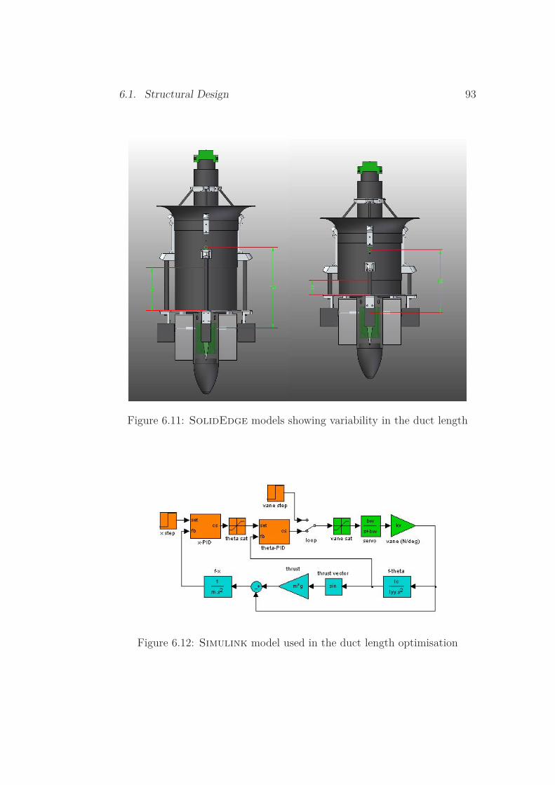
6.1. Structural Design 93
Figure 6.11: SolidEdge models showing variability in the duct length
Figure 6.12: Simulink model used in the duct length optimisation

94 6. Mechanical Design
Figure 6.13: Plots of open and closed loop step responses

6.1. Structural Design 95
6.1.5.2 Central Hub
The central hub provided a suitable place to house some of the auxiliarycomponents. The PicoPic, 7.4V lithium polymer battery and the 3DM-GX1IMU were all small enough to fit within the central hub. This was mostadvantageous as this configuration allowed these components to be housedsafely at the vertical axis of symmetry in a region which was required to bevoid from air flow.
The central hub was primarily composed of acrylic tubing, with turnedPVC fittings and a prefabricated aerodynamic end cap, as seen in Figure 6.7.Originally it was thought to construct the hub from cardboard to reduceweight. However cardboard proved difficult to work with, while the acrylictubing was rigid and provided a readymade and accurate cylindrical profile.Figure 6.14 highlights the central hub and where the PicoPic, 7.4V lithiumpolymer battery and the 3DM-GX1 IMU are housed.
Figure 6.14: Photograph of components assembled inside the acrylic hub
6.1.5.3 Duct Extension
As previously mentioned, the duct extension was not required to bear struc-tural loads. It was required to be lightweight whilst providing a rigid wall

96 6. Mechanical Design
to contain the flow. Hence it was constructed from cardboard sheets coatedin resin. The outer diameter was matched to the inner diameter of the fanduct such that it fit securely within the fan, butting up against the statorvanes. Figure 6.15 shows the duct piece being fitted into the fan and thebottom end fixings.
Figure 6.15: Photograph of the outside duct fitting into the fan
6.1.6 Landing RigIt was required to design a structural system to act as landing gear forthe craft, as well as a crash mitigation system. Criteria for design were asfollows:
• The system is required to orient the craft perfectly vertically whilston the ground, providing sufficient clearance for the duct efflux so asto reduce the impact of ground effects.
• The system is required to protect the craft during crash for all orien-tations. This should include a means of shock absorption.
• The system is to be as lightweight as possible, so as to have minimalbearing on vehicle dynamics.
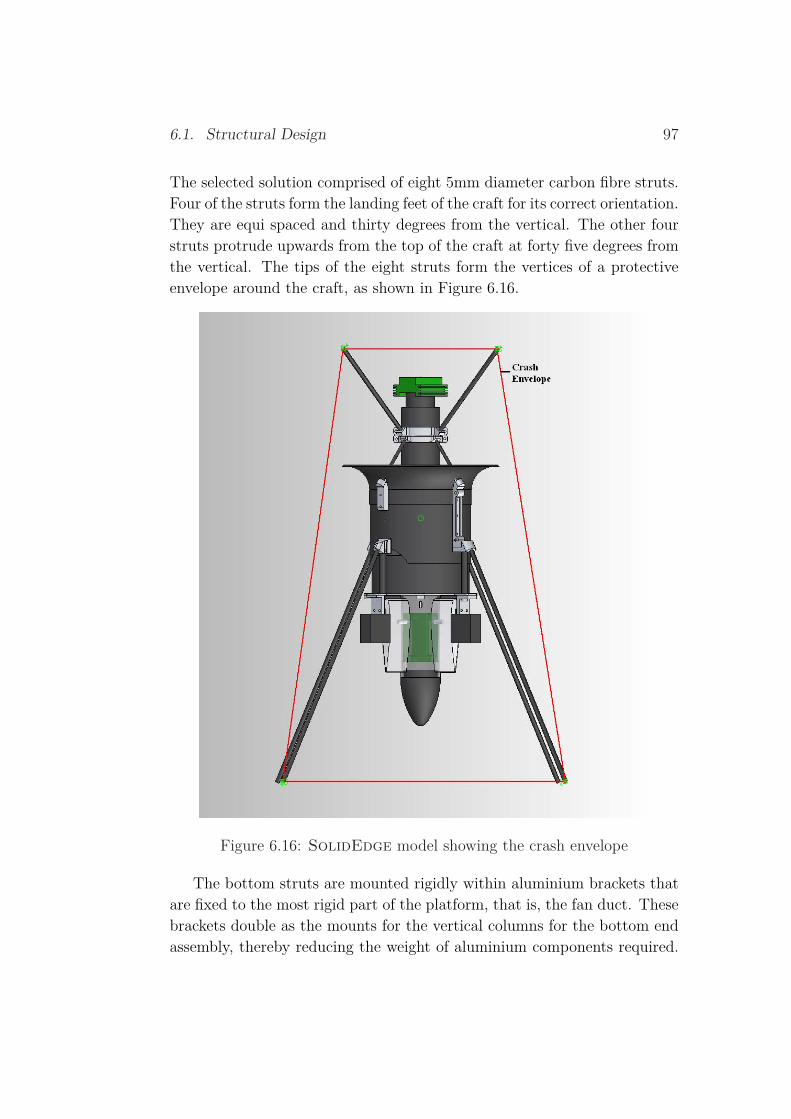
6.1. Structural Design 97
The selected solution comprised of eight 5mm diameter carbon fibre struts.Four of the struts form the landing feet of the craft for its correct orientation.They are equi spaced and thirty degrees from the vertical. The other fourstruts protrude upwards from the top of the craft at forty five degrees fromthe vertical. The tips of the eight struts form the vertices of a protectiveenvelope around the craft, as shown in Figure 6.16.
Figure 6.16: SolidEdge model showing the crash envelope
The bottom struts are mounted rigidly within aluminium brackets thatare fixed to the most rigid part of the platform, that is, the fan duct. Thesebrackets double as the mounts for the vertical columns for the bottom endassembly, thereby reducing the weight of aluminium components required.

98 6. Mechanical Design
Two of the brackets are adapted to bolt rigidly to the long duct brackets,utilising the vertical column as a bolt, as shown in Figure 6.17. The otherpair of brackets is fixed to the fan duct itself. In order to distribute theimpulsive loading from the struts, these brackets were fixed with two pairsof screws spaced vertically. This reduces the loads on the duct wall in orderto prevent fracture, as shown in Figure 6.18.
Figure 6.17: SolidEdge model of the adapted landing bracket(1) adapted landing bracket, (2) long duct bracket, (3) vertical column, (4)landing strut
The top struts are mounted rigidly within an aluminium clamp thatfixes to motor, as shown in Figure 6.16. This clamp butts against themotor mount clamp, ensuring that impulsive loads are dissipated throughrigid motor mount structure. It is intended that the elasticity of carbonfibre struts under bending will aid in absorbing impulsive loads, therebyprotecting components. Polystyrene balls were incorporated as feet to pro-vide further shock absorption.
6.2 CommissioningAfter construction, it was required to commission the craft statically toverify its structural, mechanical and electrical integrity. The main compo-

6.2. Commissioning 99
Figure 6.18: SolidEdge model of the independent landing bracket
nents of interest were the rotor and the motor mounts. The commissioningprocess went as follows. The vehicle was mounted rigidly by the long ductbrackets to a fixed structure. The motor was then run at low speeds toinspect for rubbing of fan blade tips on the duct or excessive vibration. Itwas then ramped up to and in excess of anticipated operating speeds toinspect the full range of operation. Inspection revealed no rubbing and thestructural integrity appeared sound. Motor winding temperature was mon-itored throughout the process to ensure that it remained within the boundsspecified by Plettenberg. Increasing winding temperature dictated the needfor limited operating periods followed by cooling periods during which themotor is run at low speed.
During this process it was noted that the motor-fan system emittedtwo distinct audible tones, one of which seemed to resonate at a distinctoperating speed during ramp up. It was decided that vibrational spectrawere required to inspect the mechanical integrity of system.
The spectra were produced using a single axis accelerometer mountedon the bearing housing along with a spectrum analysis software package.An example of the spectra examined is shown in Figure 6.19, which wastaken at an operating speed in the order of 8000rpm, which corresponds toan approximate run speed frequency of 140Hz. The low frequency range

100 6. Mechanical Design
of this spectrum shows many harmonics of run speed, but also includes abroad range component of lower amplitude. The run speed harmonics werelikely a result of minor imbalance or misalignment. These peaks are ofsmall magnitude so they were not a concern. The broadband componentwas thought to be a structural resonance that emitted the low frequencyaudible tone. This tone resonated well below the required operating speed,thus it was not an issue.
Figure 6.19: Plot of spectra taken at a run speed of 140 Hz
During the latter stages of testing, a problem arose in the failure of theESC. The failure was not due to an isolated incident, but was thought tohave resulted from a number of issues including:
• Excessive current transients - the controller is not designed to be runwith a mains powered DC supply. Large current transients may haveoverloaded components.
• Excessive vibration - the controller was mounted directly to the mo-tor and as such was subject to vibrations which may have fatiguedsoldered joints.
• Inappropriate settings - the switching rate was set at a low settingand the timing advance high. These settings were not appropriate forlow inductance motors such as the Plettenberg HP 370 50 A1 S.
Following the purchase of a replacement speed controller, the following mea-sures were taken to avoid a repeat failure:
• A large capacitor, 31,000µF, see Figure 6.20, was placed in series withthe power supply to protect the load from excessive current transients.
• A neoprene vibration isolator was fitted between the motor and speedcontroller.
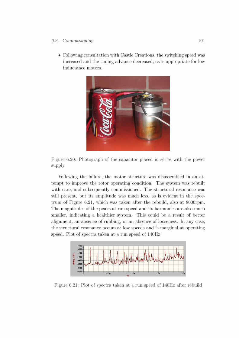
6.2. Commissioning 101
• Following consultation with Castle Creations, the switching speed wasincreased and the timing advance decreased, as is appropriate for lowinductance motors.
Figure 6.20: Photograph of the capacitor placed in series with the powersupply
Following the failure, the motor structure was disassembled in an at-tempt to improve the rotor operating condition. The system was rebuiltwith care, and subsequently commissioned. The structural resonance wasstill present, but its amplitude was much less, as is evident in the spec-trum of Figure 6.21, which was taken after the rebuild, also at 8000rpm.The magnitudes of the peaks at run speed and its harmonics are also muchsmaller, indicating a healthier system. This could be a result of betteralignment, an absence of rubbing, or an absence of looseness. In any case,the structural resonance occurs at low speeds and is marginal at operatingspeed. Plot of spectra taken at a run speed of 140Hz
Figure 6.21: Plot of spectra taken at a run speed of 140Hz after rebuild

102 6. Mechanical Design
6.3 Aerodynamic DesignThe aerodynamic design of the craft is of great importance. In order toprovide thrust efficiency and sufficient attitude control authority, all of thecomponents located in areas of air flow generated from the ducted fan weregiven aerodynamic consideration. This section outlines the pressure lossesassociated with component geometries and the design of the control vanes.
6.3.1 Ducted Fan
As previously discussed in Section 3.3, the purchase of a larger ducted fanor the construction of a ducted propeller arrangement was not feasible con-sidering the time frame of the project.
Air may be regarded as an incompressible gas, provided that the Machnumber of the flow speed is less than 0.3 (Munson et al., 2002). At flowspeeds greater than this, the incompressible flow model may begin to differfrom the compressible flow model. Thus, it was important to determine theestimated maximum flow speed within the ducted fan to see if compress-ibility effects would be indeed important.
All viscous fluids have no-slip boundary conditions. In other words, thethin surface of air in contact with the rotor blade area also travels at thesame speed as the rotor. Thus, the maximum air speed inside the ductedfan will correspond with the maximum rotor tip speed generated by themotor.
It was found that the rotor tip speed required to generate 0.3 of thespeed of sound (onset of compressibility - (Munson et al., 2002)) was approx-imately 15,120rpm. The relevant calculations are shown in Appendix C.1.Prior to testing, this fan speed was considered to be a limiting factor on fanefficiency. It was expected that at fan speeds greater than say 15,000rpm,the thrust-speed curve would begin to plateau and no longer fit a typicalparabolic curve. This phenomenon is often referred to as the “fan ceiling”,where the compressibility of air prevents further thrust from the fan andthus changing the expected parabolic thrust speed curve into an “S” shapedcurve. This is depicted in Figure 6.22.
In practice, this phenomenon was not noticed. This is most likely dueto the fact that at 0.3 of the speed of sound, the flow may indeed becomecompressible, yet the effects of compressibility may not be pronounced such

6.3. Aerodynamic Design 103
Figure 6.22: Plot of compressible and incompressible thrust-speed schemat-ics
that a measurable decrease of fan efficiency was noticeable. It is possiblethat noticeable decreases in fan efficiency may be present at say 0.7 or 0.8of the speed of sound. This could be neglected since such fan speeds areoutside the relevant range of operation of the craft rotor speeds.
In order to predict exiting air flow speeds and volumetric flow rates fromthe craft, propeller-momentum theory was used. Using this, basic equationsrelating air speed, swept propeller area and thrust can be used to help designother aerodynamic components, such as the control vanes. The swept areais given by the difference in area between the fan rotor and the fan hub.The relevant dimensions are depicted in Figure 6.23.
The governing equation relating flow speed and thrust is shown as Equa-tion 6.3, which is based on propeller-momentum theory (Schneider, 2005).
U =
√2T
ρπ (d22 − d2
1)(6.3)
whereU = Gas velocity (m/s)T = Thrust (kg)ρ = Gas density (kg/m3)d1, d2 = Fan rotor and fan hub diameters respectively (m)

104 6. Mechanical Design
Figure 6.23: SolidEdge model of the fan rotor, top view
Equation 6.3 was verified against some experimental data. At a fanspeed of approximately 11,000rpm (equates to 1.2kg of thrust), the maxi-mum noted air speed at the craft exit was measured at 75km/hr, using ananemometer. The flow measurement was taken at a distance of 20cm fromthe exit of the craft, in order to avoid any structural effects to the air flow.Using Equation 6.3, the expected maximum airspeed was 80km/hr for thegiven conditions.
From this verification, the air speeds reaching the control vanes couldbe well approximated using propeller-momentum theory. This allowed foraccurate mathematical design and modelling of the control vanes prior toany System Identification testing and thus allowing a basic verification ofresults generated from further testing.
6.3.2 Bellmouth Inlet
In order to increase the efficiency of air flow from the surrounding air intothe ducted fan, a rounded (bellmouth) inlet was designed. Knowing thisand the importance of flow efficiency of the overall craft, a bellmouth inletwas designed. This is depicted in Figure 6.24.
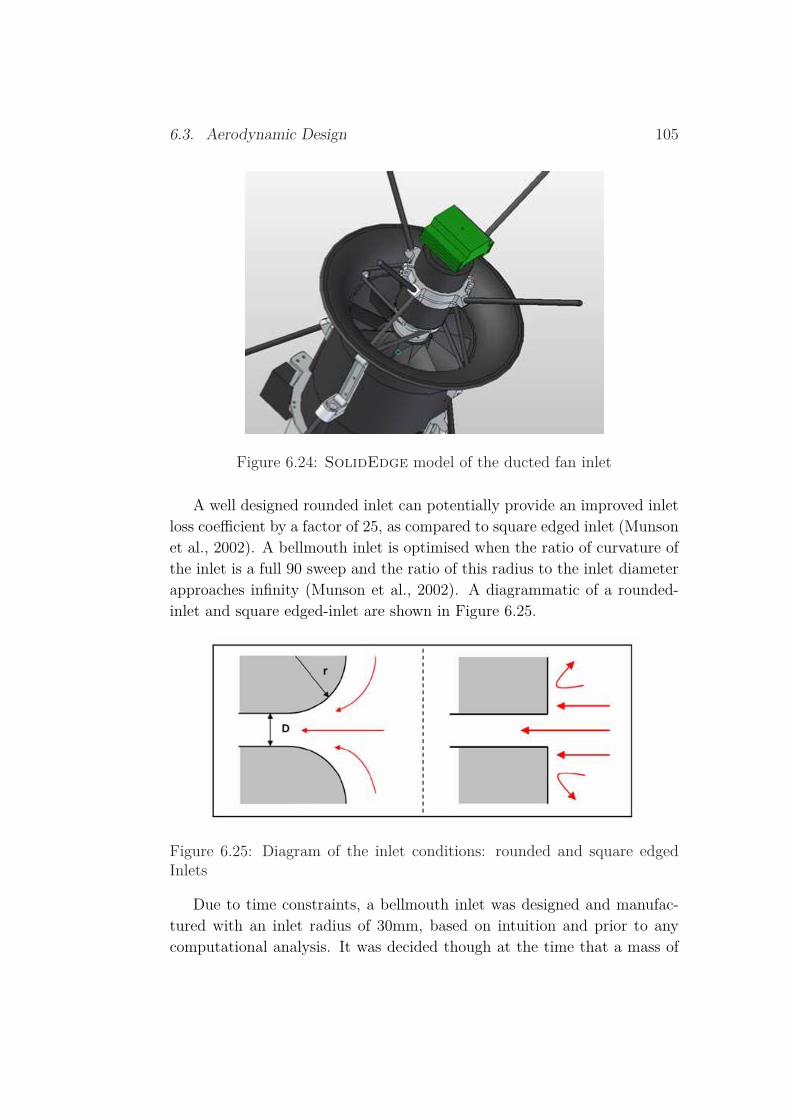
6.3. Aerodynamic Design 105
Figure 6.24: SolidEdge model of the ducted fan inlet
A well designed rounded inlet can potentially provide an improved inletloss coefficient by a factor of 25, as compared to square edged inlet (Munsonet al., 2002). A bellmouth inlet is optimised when the ratio of curvature ofthe inlet is a full 90 sweep and the ratio of this radius to the inlet diameterapproaches infinity (Munson et al., 2002). A diagrammatic of a rounded-inlet and square edged-inlet are shown in Figure 6.25.
Figure 6.25: Diagram of the inlet conditions: rounded and square edgedInlets
Due to time constraints, a bellmouth inlet was designed and manufac-tured with an inlet radius of 30mm, based on intuition and prior to anycomputational analysis. It was decided though at the time that a mass of

106 6. Mechanical Design
100g would be a design maximum. Knowing this and in conjunction withknowledge of inlet structures utilised on open wind tunnel circuits (Kelso,2006), an inlet radius to diameter ratio was chosen and formed using Solid-Edge.
At a fixed fan speed of 13,000rpm, the craft thrust was measured withand without the bellmouth inlet installed. The result is shown as follows.
Thrust: At fan speed = 13,000rpm
Without bellmouth 1.92kgWith bellmouth 2.14kg
It can be seen that there is a net thrust benefit of 220g with the inletstructure installed. Considering that the bellmouth inlet has a total mass of80g (after modifications), this lead to a mass benefit of 140g at 13,000rpm.In order to see if the deigned bellmouth inlet was optimised, a detailed inletflow analysis was performed.
Inlet pressure losses were also incurred due to the location of the motor,speed-controller and the carbon struts supporting the motor which impededinlet air flow. Obviously such complex geometries do not have empiricallyavailable data for their respective loss coefficients, yet it can be safely as-sumed that the losses due to these structural members are somewhat in-dependent of the losses associated with the bellmouth inlet. This is dueto the fact that the bellmouth inlet losses are comprised of generated wallfriction (small) and the gradual inlet contraction ratio of the air from thesurrounding air (infinite reservoir) into a finite volume. Little losses aregenerated in the centre of the airflow profile, where the motor is located,due to the bellmouth alone.
Thus, the overall inlet loss coefficient can safely be expressed as a linearalgebraic sum of the loss coefficients of the bellmouth and the structuralmembers, including the motor, struts and speed-controller. From this result,a pressure loss analysis based on the bellmouth inlet geometry alone wasperformed, in order to optimise inlet flow conditions. As little could be doneto improve the aerodynamics of the speed controller and the motor, thebellmouth inlet was the only feasible aerodynamic inlet design parameter.
As stated earlier, the larger the bellmouth radius to inlet diameter, thesmaller the loss coefficient. However, this comes at a costly increase of
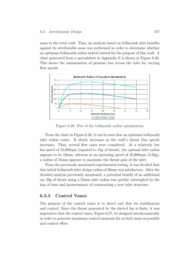
6.3. Aerodynamic Design 107
mass to the total craft. Thus, an analysis based on bellmouth inlet benefitsagainst its attributable mass was performed in order to determine whetheran optimum bellmouth radius indeed existed for the purpose of this craft. Achart generated from a spreadsheet in Appendix E is shown in Figure 6.26.This shows the minimisation of pressure loss across the inlet for varyingflow speeds.
Figure 6.26: Plot of the bellmouth radius optimisation
From the chart in Figure 6.26, it can be seen that an optimum bellmouthinlet radius exists. It slowly increases as the craft’s thrust (fan speed)increases. Thus, several flow cases were considered. At a relatively lowfan speed of 10,000rpm (equated to 1kg of thrust), the optimal inlet radiusappears to be 10mm, whereas at an operating speed of 16,000rpm (2.5kg),a radius of 25mm appears to maximise the thrust gain of the inlet.
From the previously mentioned experimental testing, it was decided thatthis initial bellmouth inlet design radius of 30mm was satisfactory. After thedetailed analysis previously mentioned, a potential benefit of an additionalsay 20g of thrust using a 25mm inlet radius was quickly outweighed by theloss of time and inconvenience of constructing a new inlet structure.
6.3.3 Control VanesThe purpose of the control vanes is to divert exit flow for stabilizationand control. Since the thrust generated by the ducted fan is finite, it wasimperative that the control vanes, Figure 6.27, be designed aerodynamicallyin order to generate maximum control moments for as little mass as possibleand control effort.

108 6. Mechanical Design
Figure 6.27: SolidEdge model showing the control vanes
The important geometric parameters of the control vanes are length (L),width (t) and thickness (W). In determining the surface for lift force andhence control moment generation, only length and width are significant.The thickness only significantly affects the drag of each control vane ina neutral position (zero angle of attack). The geometric parameters aredepicted in Figure 6.28.
Figure 6.28: Diagram of the control vane geometric parameters
Lift and drag forces are always generated simultaneously for all flowconditions and angles of attack. The lift force acts perpendicularly withrespect to the oncoming flow field and the drag force always opposes the

6.3. Aerodynamic Design 109
flow direction. Note that the directions of lift and drag are not altered bythe angle of attack of the aerofoil.
The magnitudes of the control moments able to be generated from anaerofoil are dependent upon their coefficients of lift and drag within a rel-evant control range of 20 degrees. Thus it was imperative that the controlvanes be based on existing aerofoils which had well documented, effectivelift and drag characteristics. From detailed research and computationalflow analysis (see Appendix D.1), they were designed based on a NACA0015 aerofoil (AerospaceWeb, 2006). The empirical data available for thelift and drag coefficients of these aerofoils occurred under very similar flowconditions generated by the ducted fan at high fan speeds. In addition, thisparticular aerofoil is symmetric, which allows for identical flow character-istics and hence control moments for both negative and positive angles ofattack. The lift and drag coefficients can be seen in Figure 6.29.
Using the known lift and drag coefficients of the aerofoil profiles, thecontrol force from each vane could be approximated using 2D aerofoil theory.Equation 6.4, was used to determine the lift force per control vane. Thederivation may be found in Appendix D.1.
F =1
2ρLU2
(D2 − d2
1
)(mα)sinα
(t
[2t + h]2
)(6.4)
whereF = Lift force (N)D = Duct diameter (m)m = Linearised lift coefficient (1/rad)α = Angle of attack (rad)t = Control vane width (m)h = Central hub diameter (m)
From this equation and the plots shown in Figure 6.29, it can be seenthat the control vane force response for an angular input is highly non-linear. This is typical of most aerodynamic systems. In addition, it can beseen that the generated lift force per vane is directly proportional to thearea of the vane (area seen by the oncoming flow field). From Equation 6.4,it can be seen that the only design parameter of control is essentially thecontrol vane area (after the selection of an appropriate aerofoil profile).
Despite its simplicity, the 2D aerofoil theory has several limitations in
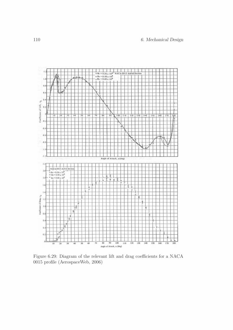
110 6. Mechanical Design
Figure 6.29: Diagram of the relevant lift and drag coefficients for a NACA0015 profile (AerospaceWeb, 2006)

6.3. Aerodynamic Design 111
predicting realistic flow fields and lift forces. Some of the limitations includethat the lift coefficient is usually empirically determined upon a wing withan aspect ratio (width to length ratio) of at least 5–10. The aspect ratioof the control vanes employed by the craft are approximately 0.4. It isunknown how this will affect the realistic lift coefficient plot with respect toangle of attack. It is predicted that the stall angle will increase significantlyand that the maximum lift coefficient will be achieved at a higher angleof attack than suggested by the NACA 0015 plots, shown previously inFigure 6.29.
The 2D theory does not take into account the irregularities of the flowpattern onto the control vanes. The flow is highly turbulent and highlyrotational. This is due to the nature of the exiting air from the ductedfan. In the published lift coefficient data, it is assumed that the air flow isturbulent and fully-developed. As will be shown in Section 6.3.4, the flowreaching the control vanes is not fully-developed and thus the control forceresponse will most likely be overestimated.
In reality, the flow past an aerofoil at relatively high Reynolds numberflow generally has an associated wake. The wake comprises of highly viscousfluid flow, with eddies and rotational patterns. This in turn leads to anincreased overall drag coefficient for the aerofoil, which in turn decreases theoverall thrust efficiency of the craft. The only method to combat this issuewas to employ an aerofoil profile which has a relatively low drag coefficientat a zero angle of attack. The NACA 0015 profile manages to provide this.
In general, the 2D theory should not be used exclusively to determine liftand drag forces on real aerofoils, especially those with expected rotationalflow inputs and low aspect ratios. This is best depicted diagrammatically;some of the previously outlined issues are displayed in Figures 6.30 & 6.31.They display both planform and side views respectively of predicted flowpatterns using 2D Theory and expected flow patterns in reality.
The use of 2D aerofoil theory is most likely accurate to within a 50%design estimate, thus in determining the expected control vane force, theresult generated from Equation 6.4 should really be halved to give a moreaccurate control vane response.
Taking the limitations and realities of the ducted fan air flow into ac-count, the control vane geometries could be designed. This proved not to assimple a task as it seems, as it was difficult to determine what magnitudeof control moment is required in free space in order to control the craft in

112 6. Mechanical Design
Figure 6.30: Diagram of a planform view of predicted and expected flowpatterns
Figure 6.31: Diagram of a side view of predicted and expected flow patterns

6.3. Aerodynamic Design 113
hover. Nonetheless, it was determined that 1N of thrust per control vanewould be sufficient for control purposes (Cazzolato, 2006). In addition tobeing able to meet the control moment requirements, it was important thatsuch a control force could be attained at a small of an angle of attack aspossible. This would allow for more flexibility in designing a controller andthus making it potentially more robust to larger magnitude disturbancesand coupling effects.
After a detailed aerofoil and flow analysis, control vane dimensions wereselected. These were based upon the radius of curvature of the NACA 0015profile and the required surface area of the aerofoil to generate a sufficientcontrol moment. The NACA 0015 profile is based upon a generic equationemployed by NACA and the 0015 represent coefficients of parameters inputinto the equation. The curvature profile generated in Matlab and latertransferred to SolidEdge is shown in Figure 6.32. Details of the governingequation and the associated generation of the control vane model is locatedin Appendix D.3.
Figure 6.32: SolidEdge model of the NACA 0015 interpolation
Upon design of the control vanes, careful consideration was given to theirlocation. It was important that there was sufficient room for the vanes todivert flow outside the duct, yet at the same time it was important that thevanes were not too far out of the duct such that air would dissipate intofree space prior to reaching the aerofoil surface.
The placement of the vanes relative to the length of the duct as previ-ously described is very important during control manoeuvres which requirerelatively large angles of attack for control. Locating the vanes within theduct would throttle the flow, reducing vane effectiveness and also thrust.Conversely, if the tip of the control vane was located lower than the ductexit, kinetic energy would be dispersed. Both cases are depicted in Fig-ure 6.33.
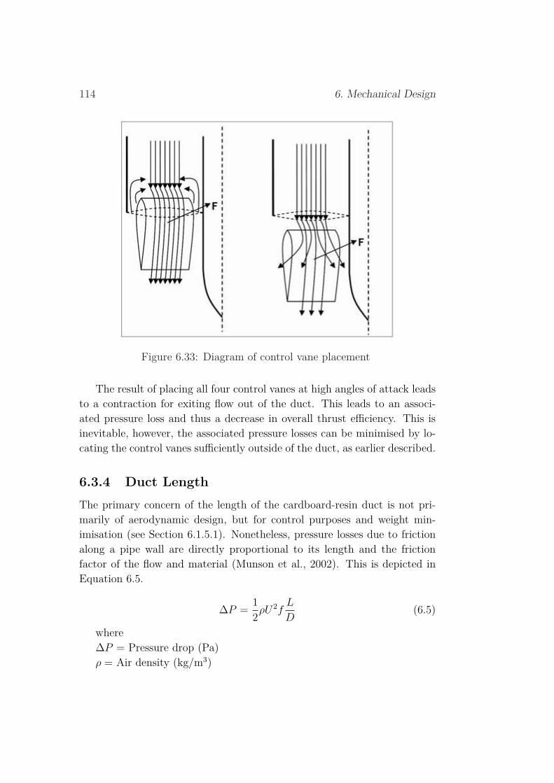
114 6. Mechanical Design
Figure 6.33: Diagram of control vane placement
The result of placing all four control vanes at high angles of attack leadsto a contraction for exiting flow out of the duct. This leads to an associ-ated pressure loss and thus a decrease in overall thrust efficiency. This isinevitable, however, the associated pressure losses can be minimised by lo-cating the control vanes sufficiently outside of the duct, as earlier described.
6.3.4 Duct LengthThe primary concern of the length of the cardboard-resin duct is not pri-marily of aerodynamic design, but for control purposes and weight min-imisation (see Section 6.1.5.1). Nonetheless, pressure losses due to frictionalong a pipe wall are directly proportional to its length and the frictionfactor of the flow and material (Munson et al., 2002). This is depicted inEquation 6.5.
∆P =1
2ρU2f
L
D(6.5)
where∆P = Pressure drop (Pa)ρ = Air density (kg/m3)

6.3. Aerodynamic Design 115
U = Air speed (m/s)f = Friction factorL = Duct length (m)D = Duct diameter (m)
Since the inside of the duct was quite smooth and that the duct lengthwas also quite short, the frictional losses due to duct length were assumednegligible.
The length of the duct was also investigated to see whether the possi-bility of fully-developed flow could be attained prior to reaching the controlvanes. This would have been beneficial, as this would allow for a more uni-form profile of air passing over the vanes, thus making the vane responsemore reliable.
The length of duct required for fully developed flow was significantlygreater than any realistic duct length possible (see Appendix C.2). Due tothis, the length of the duct was chosen based upon structural and controlrequirements.
6.3.5 Duct WidthIn order to optimise control moments, the width of the duct and hence thewidth of the control vanes was investigated. Three cases were considered:Ducted fan width and narrow/wider than fan width. The latter two aredepicted in Figure 6.34.
Using 2D aerofoil theory and basic fluid mechanics (continuity equation,neglecting pressure losses), an optimum control vane width was determined.The analysis assumed for all flow conditions that the inlet conditions andcontrol vane lengths were the same. In addition, it is also assumed that theduct width is equal to the sum of two control vane widths and the centralhub diameter. The resulting plot is shown in Figure 6.35 (the analysis andresults may be found in Appendix D.2).
As it can be seen from Figure 6.35, there indeed exists an optimum ductwidth such that the control vane moment is maximised. The reason forthe dimensionless control moment is based on a proportionality analysis.It should be noted that in general, using this methodology the optimumcontrol vane width is half that of the central hub diameter. This can bedetermined by differentiating Equation 6.6.

116 6. Mechanical Design
Figure 6.34: Diagram of duct width analysis
Figure 6.35: Plot of control vane width optimisation (2D Theory)
6.3. Aerodynamic Design 117
F ∝ t
(2t + h)2 (6.6)
whereF = Control vane force (N)t = Control vane width (m)h = Central hub diameter (m)
In practice, 3D effects such as turbulence, wing-tip vortices and pressurelosses due to sudden contractions/expansions in duct area will change theshape of the optimisation plot. It is expected that the optimum duct widthwill approach the width of the ducted fan at high fan speeds. This is dueto the fact that pressure losses are proportional to inlet velocity squared,whereas increases in area only change the air speed linearly (by conservationof mass for an incompressible fluid). Considering this and the associateddifficulty with installing a bottom assembly with diameter smaller than thatof the ducted fan, the duct diameter was chosen to be the same as the ductedfan (ie, no change in duct cross sectional area).
6.3.6 Central Hub
The primary function of the central hub is to house various hardware com-ponents, as described in Section 6.1.5.2. From an aerodynamic perspective,the hub was designed such that there were as few changes in hub diameteralong its respective length as possible. This was done in order to minimiseany losses associated with sudden changes in area to the flow annulus. Also,the straight section of the hub allowed for a more linear velocity profile ofair to flow past the control vanes.
In addition, the hub diameter was minimised for mass requirements. Inturn, this minimisation led to a smaller outer surface area of the hub section,thus minimising the interruption to the highly rotational exit flow from theducted fan and wall friction surface area.
6.3.7 Duct Exit
The exit loss coefficient of a pipe into an infinite reservoir of fluid is fixed,independent of exit geometry (Munson et al., 2002). Knowing this, the
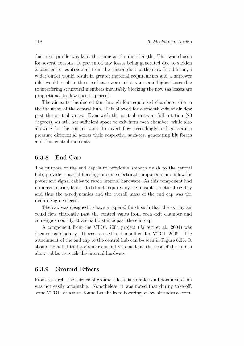
118 6. Mechanical Design
duct exit profile was kept the same as the duct length. This was chosenfor several reasons. It prevented any losses being generated due to suddenexpansions or contractions from the central duct to the exit. In addition, awider outlet would result in greater material requirements and a narrowerinlet would result in the use of narrower control vanes and higher losses dueto interfering structural members inevitably blocking the flow (as losses areproportional to flow speed squared).
The air exits the ducted fan through four equi-sized chambers, due tothe inclusion of the central hub. This allowed for a smooth exit of air flowpast the control vanes. Even with the control vanes at full rotation (20degrees), air still has sufficient space to exit from each chamber, while alsoallowing for the control vanes to divert flow accordingly and generate apressure differential across their respective surfaces, generating lift forcesand thus control moments.
6.3.8 End Cap
The purpose of the end cap is to provide a smooth finish to the centralhub, provide a partial housing for some electrical components and allow forpower and signal cables to reach internal hardware. As this component hadno mass bearing loads, it did not require any significant structural rigidityand thus the aerodynamics and the overall mass of the end cap was themain design concern.
The cap was designed to have a tapered finish such that the exiting aircould flow efficiently past the control vanes from each exit chamber andconverge smoothly at a small distance past the end cap.
A component from the VTOL 2004 project (Jarrett et al., 2004) wasdeemed satisfactory. It was re-used and modified for VTOL 2006. Theattachment of the end cap to the central hub can be seen in Figure 6.36. Itshould be noted that a circular cut-out was made at the nose of the hub toallow cables to reach the internal hardware.
6.3.9 Ground Effects
From research, the science of ground effects is complex and documentationwas not easily attainable. Nonetheless, it was noted that during take-off,some VTOL structures found benefit from hovering at low altitudes as com-

6.3. Aerodynamic Design 119
Figure 6.36: SolidEdge model of the end cap and actual end cap attachedto the craft
pared to higher altitudes. It was also noted that some difficulties duringtake-off may be present when a smooth, flat, rigid surface is not placed di-rectly beneath the craft (Lipera et al., 2001). This is shown in Figure 6.37which shows the iStar (Lipera et al., 2001) attempting a take-off from anon-uniform surface.
Figure 6.37: Photograph of ground effects on the iStar (Lipera et al., 2001)

120 6. Mechanical Design
The control of the craft could also be jeopardized if it hovers at lowaltitude. This is due to the recirculation of reflected air from the floor, backonto the duct exit. It is predicted that the recirculated flow would be highlyturbulent, irregular and also highly rotational, which would have a signifi-cant impact on the ability of the control vanes to generate control moments.This is due to the air flowing past the control vanes would interfere with therecirculated air and thus decreasing the lift effect from each control vane.
6.4 Tether DesignThe tether was required to transmit power and control signals to and fromthe craft with the minimum of impact on its dynamics. Design criteria wereas follows:
• The power cables were required to safely carry a nominal current of75A without excessive voltage drop. They were also required to be aslight as possible.
• The insulation was also required to be as light as possible. It wasalso required to be as flexible as possible so as to provide minimalconstraint on the motion of the vehicle.
• The power cables were required to feed into the end cap to preventit from destabilising the craft. This configuration will in fact increaseattitude stability as it behaves like a weak spring that restores thevehicle to its hover orientation, refer to Figure 6.38.
• Communications cables were required to be minimal in weight andstiffness.
A copper braid of appropriate current capacity was used for the powercables. A soft fibre-glass sleeve was used to insulate the cable. This provideda flexible and lightweight solution that satisfied the electrical requirements.A photograph of the cable is shown in Figure 6.39 along with the othertether cables.
The communications cabling was minimised by using a single RS232cable to transmit both actuator control signals to the craft and transducersignals from the craft as discussed in Section 4.2.4.3.
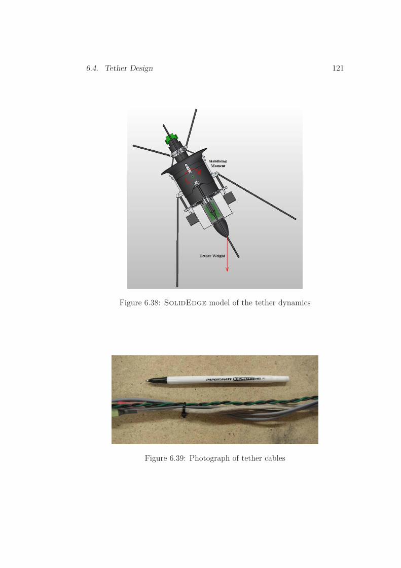
6.4. Tether Design 121
Figure 6.38: SolidEdge model of the tether dynamics
Figure 6.39: Photograph of tether cables

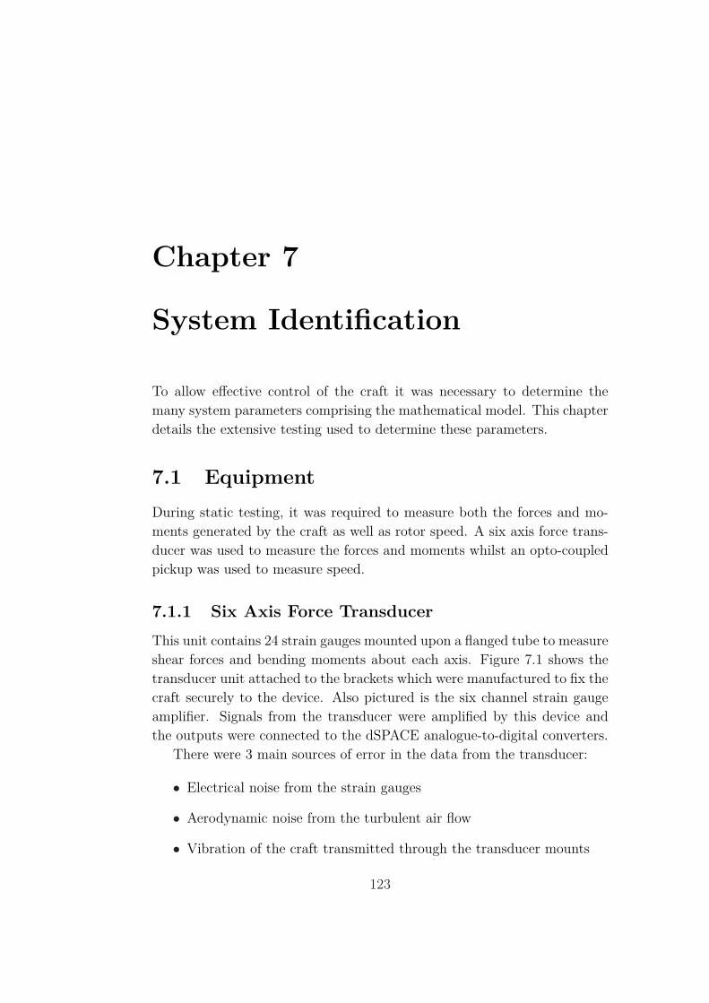
Chapter 7
System Identification
To allow effective control of the craft it was necessary to determine themany system parameters comprising the mathematical model. This chapterdetails the extensive testing used to determine these parameters.
7.1 EquipmentDuring static testing, it was required to measure both the forces and mo-ments generated by the craft as well as rotor speed. A six axis force trans-ducer was used to measure the forces and moments whilst an opto-coupledpickup was used to measure speed.
7.1.1 Six Axis Force TransducerThis unit contains 24 strain gauges mounted upon a flanged tube to measureshear forces and bending moments about each axis. Figure 7.1 shows thetransducer unit attached to the brackets which were manufactured to fix thecraft securely to the device. Also pictured is the six channel strain gaugeamplifier. Signals from the transducer were amplified by this device andthe outputs were connected to the dSPACE analogue-to-digital converters.
There were 3 main sources of error in the data from the transducer:
• Electrical noise from the strain gauges
• Aerodynamic noise from the turbulent air flow
• Vibration of the craft transmitted through the transducer mounts
123
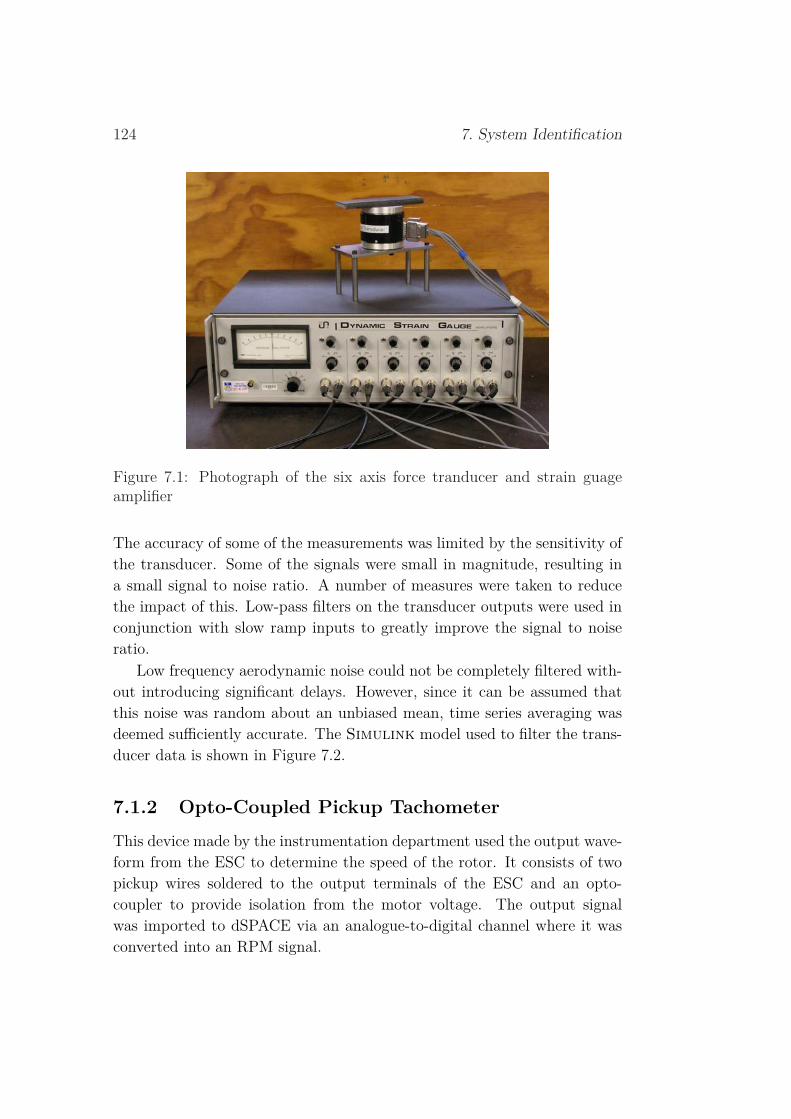
124 7. System Identification
Figure 7.1: Photograph of the six axis force tranducer and strain guageamplifier
The accuracy of some of the measurements was limited by the sensitivity ofthe transducer. Some of the signals were small in magnitude, resulting ina small signal to noise ratio. A number of measures were taken to reducethe impact of this. Low-pass filters on the transducer outputs were used inconjunction with slow ramp inputs to greatly improve the signal to noiseratio.
Low frequency aerodynamic noise could not be completely filtered with-out introducing significant delays. However, since it can be assumed thatthis noise was random about an unbiased mean, time series averaging wasdeemed sufficiently accurate. The Simulink model used to filter the trans-ducer data is shown in Figure 7.2.
7.1.2 Opto-Coupled Pickup Tachometer
This device made by the instrumentation department used the output wave-form from the ESC to determine the speed of the rotor. It consists of twopickup wires soldered to the output terminals of the ESC and an opto-coupler to provide isolation from the motor voltage. The output signalwas imported to dSPACE via an analogue-to-digital channel where it wasconverted into an RPM signal.

7.1. Equipment 125
Figure 7.2: Simulink model showing low pass filters applied to the rawtransducer data
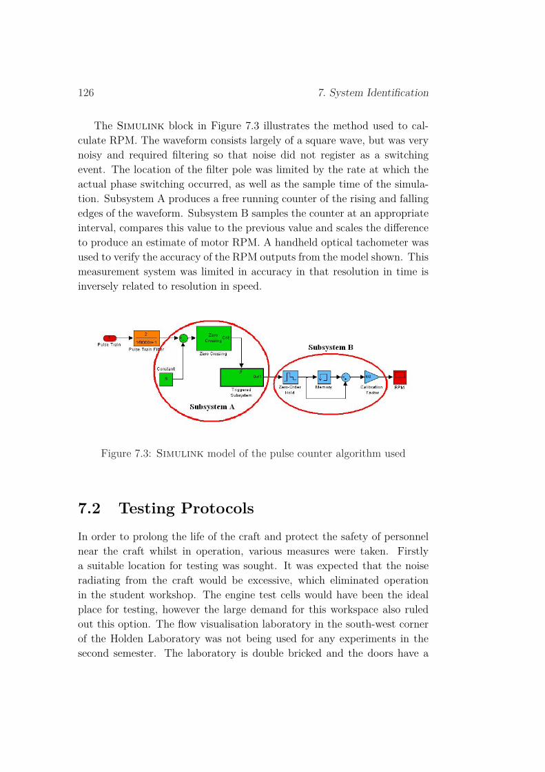
126 7. System Identification
The Simulink block in Figure 7.3 illustrates the method used to cal-culate RPM. The waveform consists largely of a square wave, but was verynoisy and required filtering so that noise did not register as a switchingevent. The location of the filter pole was limited by the rate at which theactual phase switching occurred, as well as the sample time of the simula-tion. Subsystem A produces a free running counter of the rising and fallingedges of the waveform. Subsystem B samples the counter at an appropriateinterval, compares this value to the previous value and scales the differenceto produce an estimate of motor RPM. A handheld optical tachometer wasused to verify the accuracy of the RPM outputs from the model shown. Thismeasurement system was limited in accuracy in that resolution in time isinversely related to resolution in speed.
Figure 7.3: Simulink model of the pulse counter algorithm used
7.2 Testing ProtocolsIn order to prolong the life of the craft and protect the safety of personnelnear the craft whilst in operation, various measures were taken. Firstlya suitable location for testing was sought. It was expected that the noiseradiating from the craft would be excessive, which eliminated operationin the student workshop. The engine test cells would have been the idealplace for testing, however the large demand for this workspace also ruledout this option. The flow visualisation laboratory in the south-west cornerof the Holden Laboratory was not being used for any experiments in thesecond semester. The laboratory is double bricked and the doors have a

7.3. Static Testing 127
high sound transmission class rating which dampened the noise from thecraft. There is little thoroughfare in the vicinity of this laboratory and thecraft could be operated in isolation, away from bystanders. This laboratorywas therefore used for the bulk of testing. In order to protect the existingequipment in the laboratory, barriers were erected to segment the craft fromthe equipment. Windows were required to be installed in the door in orderto visually inspect the craft under operation external to the laboratory asno other accessible windows to the laboratory were available.
During testing a few measures were taken to protect both the craft andnearby personnel:
• Motor temperature was constantly monitored with a thermocouplelocated near the motor windings.
• After a lengthy high speed test, the motor was cooled down by runningat low speed until the temperature returned to a safe level quoted byPlettenberg.
• An isolation power switch was used inline to the motor to engagecutoff when overloaded.
• Structural resonances were passed through quickly to prevent exces-sive vibrations.
• During high speed testing, all personnel were required to vacate thelaboratory.
• Hearing protection was to be worn for all testing with eye protectionadditional for personnel inside the laboratory.
7.3 Static TestingThe first phase of testing was static testing during which the craft wasrigidly mounted to the transducer as shown in Figure 7.4. The craft wasmounted to the transducer by means of a steel mount. This mount consistedof four posts that bolt to the long duct brackets and a plate that bolts tothe top flange of the transducer. The bottom flange of the transducer wasbolted to another steel plate which was clamped to a section of I-beam.

128 7. System Identification
Figure 7.4: Photograph of the craft mounted to the six axis force transducer
Testing in this configuration allowed the measurement of the followingcharacteristics:
• Thrust generated as a function of rotor speed
• Yaw moment generated as a function of rotor speed
• Rotor speed dynamics
• Control vane forces generated as a function of vane angle of attack,with constant rotor speed
7.3.1 Thrust-Speed CharacteristicAn accurate relationship between fan speed and thrust was required as thebasis for altitude control. This relationship allows any thrust command tobe mapped to a speed command. It also allows the estimation of a linearisedthrust-speed characteristic about an operating point corresponding to hover.
The procedure of the experiment was to use a slow ramp signal to themotor duty cycle, such that the speed would increase linearly over an ex-tended period, minimising the impact of noise. Thrust was measured by
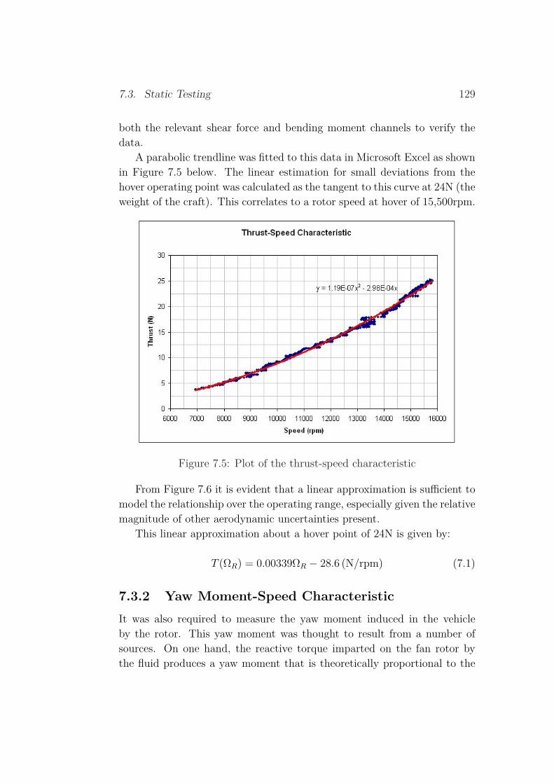
7.3. Static Testing 129
both the relevant shear force and bending moment channels to verify thedata.
A parabolic trendline was fitted to this data in Microsoft Excel as shownin Figure 7.5 below. The linear estimation for small deviations from thehover operating point was calculated as the tangent to this curve at 24N (theweight of the craft). This correlates to a rotor speed at hover of 15,500rpm.
Figure 7.5: Plot of the thrust-speed characteristic
From Figure 7.6 it is evident that a linear approximation is sufficient tomodel the relationship over the operating range, especially given the relativemagnitude of other aerodynamic uncertainties present.
This linear approximation about a hover point of 24N is given by:
T (ΩR) = 0.00339ΩR − 28.6 (N/rpm) (7.1)
7.3.2 Yaw Moment-Speed CharacteristicIt was also required to measure the yaw moment induced in the vehicleby the rotor. This yaw moment was thought to result from a number ofsources. On one hand, the reactive torque imparted on the fan rotor bythe fluid produces a yaw moment that is theoretically proportional to the

130 7. System Identification
Figure 7.6: Plot of the linearised thrust-speed characteristic about 24N
square of rotor speed. This component is partly compensated, however, bythe stator vanes. It is suggested also that the efficiency of both the fanrotor and stator vary with speed. Another source of yaw moment resultsfrom changes in rotor inertia and theoretically takes the form (notation ofChapter 5):
ΣMz =JR
Jzz
.
ΩR (7.2)
Data was collected for both a slow ramp change in speed and for astep change in speed to identify the relative impact of the load-inducedand inertia-induced components of yaw moment. The plots are shown inFigure 7.7. Evidently, a clear correlation between yaw and speed and yawand rate of change of speed did not result. This was thought to be a resultof the interdependence of the aforementioned sources and the uncertaintyin each. The small signal to noise ratio may also have compromised theresult.
An accurate estimate of the yaw moment-speed characteristic was notachieved, however, the test did give an indication of the magnitude of yawmoments required to be regulated. Because yaw is not coupled with the

7.3. Static Testing 131
(a)
(b)
Figure 7.7: Plots of yaw response to: (a) Ramp speed input, (b) Step speedinput

132 7. System Identification
other states, it should not pose stability problems and thus model accuracyis not critical.
7.3.3 Rotor Speed DynamicsThe time constant of rotor speed was estimated by applying a step changeto the duty cycle input to the ESC and capturing the RPM measurementfrom the tachometer. Figure 7.8 shows the lag, which is in the order of 1second.
Figure 7.8: Plot of speed response lag
7.3.4 Control Vane CharacteristicThe moments generated by the control vanes were also difficult to measurebecause of the lower magnitudes and the sensitivity of the transducer. Tomitigate this, all four vanes were used simultaneously to create a yaw mo-ment, which allowed for a better signal to noise ratio than testing a vaneindividually. Yaw was required to be measured as the pitch moment chan-nel also measured thrust whilst the roll moment channel was notoriouslyinaccurate. The distance from the control vane force to the centre of thetransducer was measured to yield the control vane moment arm for pitch,roll and yaw. The test was undertaken by applying a ramp input to the
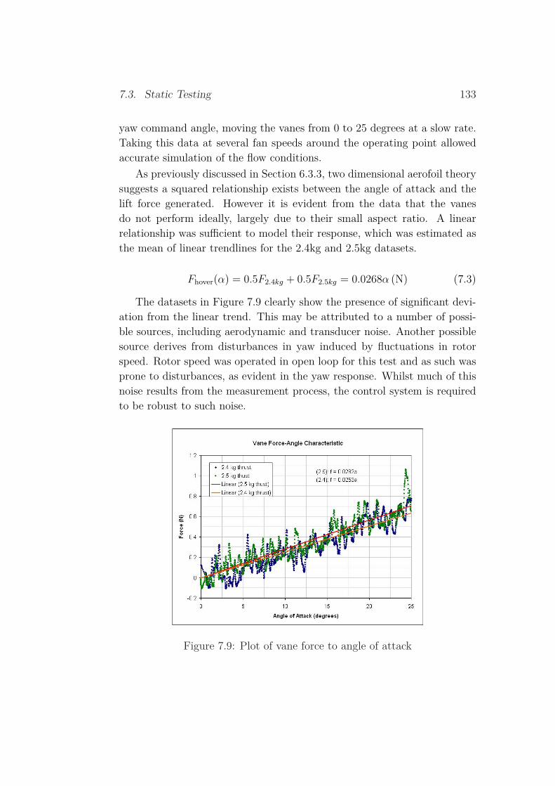
7.3. Static Testing 133
yaw command angle, moving the vanes from 0 to 25 degrees at a slow rate.Taking this data at several fan speeds around the operating point allowedaccurate simulation of the flow conditions.
As previously discussed in Section 6.3.3, two dimensional aerofoil theorysuggests a squared relationship exists between the angle of attack and thelift force generated. However it is evident from the data that the vanesdo not perform ideally, largely due to their small aspect ratio. A linearrelationship was sufficient to model their response, which was estimated asthe mean of linear trendlines for the 2.4kg and 2.5kg datasets.
Fhover(α) = 0.5F2.4kg + 0.5F2.5kg = 0.0268α (N) (7.3)
The datasets in Figure 7.9 clearly show the presence of significant devi-ation from the linear trend. This may be attributed to a number of possi-ble sources, including aerodynamic and transducer noise. Another possiblesource derives from disturbances in yaw induced by fluctuations in rotorspeed. Rotor speed was operated in open loop for this test and as such wasprone to disturbances, as evident in the yaw response. Whilst much of thisnoise results from the measurement process, the control system is requiredto be robust to such noise.
Figure 7.9: Plot of vane force to angle of attack

134 7. System Identification
7.3.5 Servo Motor Dynamics
The servo motor dynamics were required to be modelled based on frequencyresponse data. This data was collected using the same methodology dis-cussed in Chapter 4. Given that the angular amplitude and supply voltagewere significant in determining the roll-off characteristics as previously dis-cussed, this frequency response characteristic was obtained with parametersbest approximate reality. Small angular deflections of ±5 degrees were againused to simulate the low amplitude demands that are likely.
A frequency domain transfer function was created to fit the data. Asecond order model produced an excellent fit to the experimental data,which was expected based on the literature. This structure was used in apaper by Carlsson and Cronander (2004) and appears to best model servomotor dynamics.
It can be seen in Figure 7.10, the amplitude modelling is excellent butthe phase information does not exactly correspond. This was thought tobe the result of measurement delays which are not part of the dynamicsof the servo and as such were not modelled. Higher order models wereexperimented with, without a significant improvement in model accuracy.
This model has a natural frequency of ωn = 8Hz and a damping ratio,ζi = 0.7 which compares closely with the results of testing on similar servomotors in Carlsson and Cronander (2004).
7.4 Dynamic Testing
The primary aim of this phase of testing was to gauge the gyroscopic cou-pling between the pitch and roll axes and thereby estimate the inertia ofthe rotor.
7.4.1 Single Axis Testing
A single axis rig was designed and constructed that allows rotation about theroll axis. The strategy was based on the dynamics in Equations 7.4 and 7.5,utilising the notation of Chapter 5.
Jyy
..
θ = −JRΩR
.
φ (7.4)

7.4. Dynamic Testing 135
Figure 7.10: Plot of second order model against the measured data set
Jxx
..
φ = JRΩR
.
θ (7.5)
The motor was to be run at a fixed and known speed and a measuredroll rate was to be induced by a step in the roll control vanes. The gyro-scopic pitching moment was to be transmitted through the rig to the forcetransducer. A model of the craft on the rig is shown in Figure 7.11.
Figure 7.11: SolidEdge model of the single axis rig
The major difficulty with this test was that the thrust of the craft is

136 7. System Identification
measured on the same moment channel. Given the relative magnitude ofthe thrust moment and the significant fluctuation in this it was difficult toisolate the two moments.
A possible solution was to measure the thrust on both the relevant forceand moment channels. Since the gyroscopic term should only be evident inthe moment channel and the thrust in both, the difference between the twoshould simply be the gyroscopic component.
Performing this test required two conditions be met. Firstly, thrustmeasurements taken by the force and moment channels were required toaccurately correspond. Secondly, since the craft is rotating relative to thetransducer channels, measurements from multiple channels were requiredto be transformed. Slight discrepancies between the calibration of channelswould corrupt the data. Due to problems with the transducer sensitivityand accuracy, valid results were not obtained.
At this stage it was decided to pursue other methods of determiningthe rotor inertia. The motor manufacturer provided an estimate of themotor rotor inertia whilst a SolidEdge model of the fan rotor providedan estimate of this inertial component. The gyroscopic coupling was alsoto be investigated on a three degree-of-freedom rig.
7.4.2 Vehicle Centre of Gravity and Moments of In-ertia
Whilst the SolidEdge model provided an estimate of the centre of gravityand moments of inertia, many components, such as fasteners and wiring,were not accurately modelled. It was therefore necessary to determine theseparameters empirically. The vertical position of the centre of gravity waslocated by simply finding the position at which the craft balanced on a knifeedge. The control vane moment arm for pitch and roll was then accuratelydetermined as the vertical distance from this point to the centre of pressure(which corresponds to the axis of rotation) of the control vanes, that is, lθ,φ=0.125 m. The centre of gravity was assumed to lie on the axis of symmetry.
A pendulum test was conducted to determine the craft moments of in-ertia. The craft was suspended from a beam and a free oscillation wasinduced. A nominal number of oscillations were timed, from which theperiod of oscillation was determined.
The moment of inertia of a pendulum about the centre of rotation is
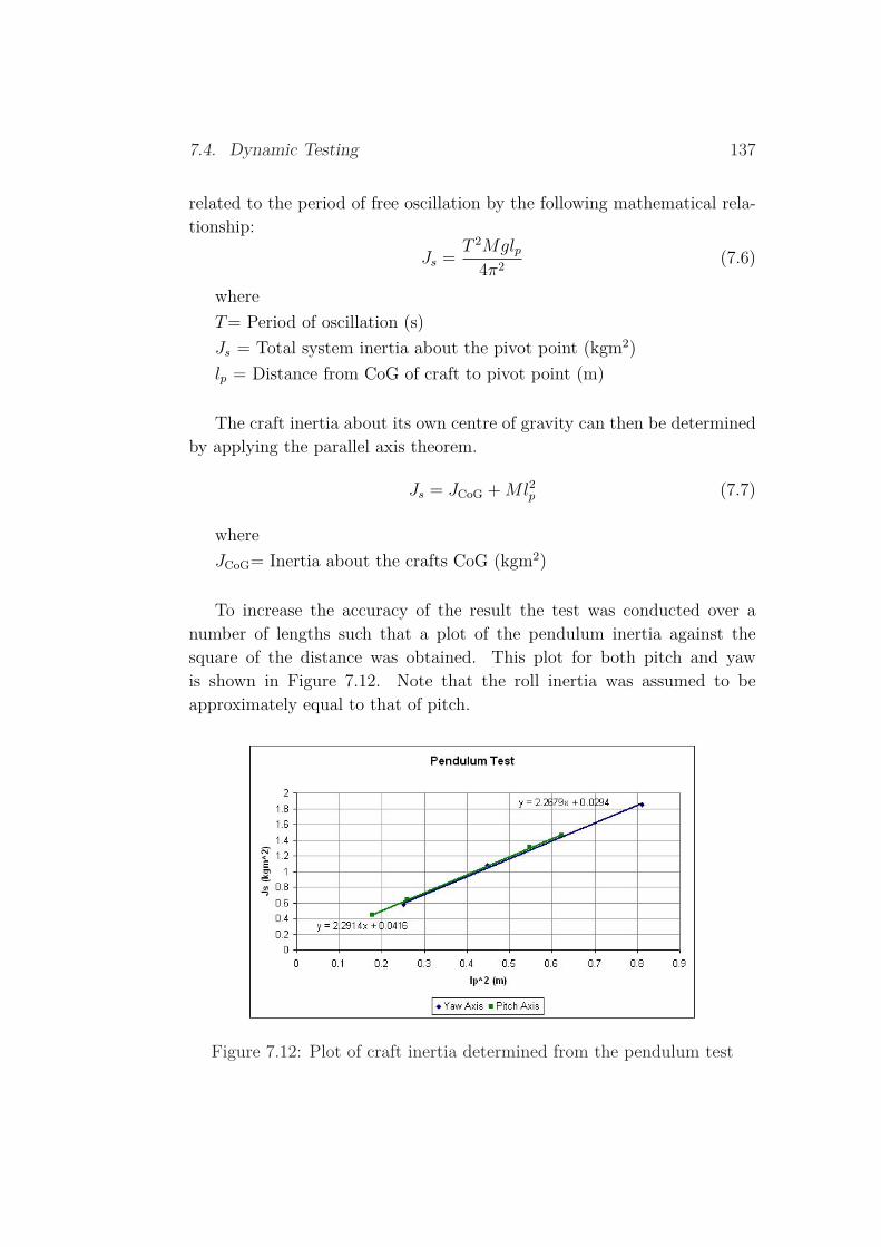
7.4. Dynamic Testing 137
related to the period of free oscillation by the following mathematical rela-tionship:
Js =T 2Mglp
4π2(7.6)
whereT= Period of oscillation (s)Js = Total system inertia about the pivot point (kgm2)lp = Distance from CoG of craft to pivot point (m)
The craft inertia about its own centre of gravity can then be determinedby applying the parallel axis theorem.
Js = JCoG + Ml2p (7.7)
whereJCoG= Inertia about the crafts CoG (kgm2)
To increase the accuracy of the result the test was conducted over anumber of lengths such that a plot of the pendulum inertia against thesquare of the distance was obtained. This plot for both pitch and yawis shown in Figure 7.12. Note that the roll inertia was assumed to beapproximately equal to that of pitch.
Figure 7.12: Plot of craft inertia determined from the pendulum test

138 7. System Identification
The craft moments of inertia were estimated as the y-axis intercept ofthe linear trendline. That is, pitch inertia, Jyy = 4.16×10⁻² kgm2 and yawinertia, Jzz = 2.94×10⁻² kgm2.
7.5 Summary of System ParametersThis section provides a summary of the parameter estimates determined byexperimentation, as well as other sources such as manufacturer’s data andthe SolidEdge model. Notation utilised within this section follows thatof Section 5.2.3.
7.5.1 Static Craft PropertiesThe mass of the craft includes all landing gear and an estimate of the weightof the tether. The detailed breakdown of the mass budget is documentedin Section 10.2.
MassM = 2.4kgPitch and Roll inertiasJxx = Jyy = 4.16×10⁻² kgm2
Yaw inertiaJzz = 2.94×10⁻² kgm2
7.5.2 Pitch and Roll ParametersThe gyroscopic coupling coefficients were determined from the rotor inertia,the relevant body inertia and the rotor speed at hover, which was assumedconstant for this purpose. The rotor inertia comprises the inertia of boththe motor and fan rotor. The motor component was obtained through cor-respondence with Plettenberg and their estimate was checked for feasibilitygiven the known mass and size of the rotor. The fan rotor was modelled inSolidEdge, and the calculated inertia value was used.
Fan rotor inertiaJfr= 8.40×10⁻⁵ kgm2
Motor rotor inertiaJmr = 4.92×10⁻⁵ kgm2
Total rotor inertia
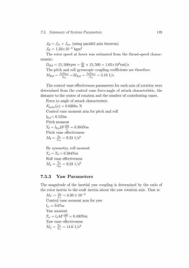
7.5. Summary of System Parameters 139
JR = Jfr + Jmr (using parallel axis theorem)JR = 1.33×10⁻⁴ kgm2
The rotor speed at hover was estimated from the thrust-speed charac-teristic:
ΩR,0 = 15, 500rpm = 2π60
× 15, 500 = 1.62×10³rad/sThe pitch and roll gyroscopic coupling coefficients are therefore:MR,θ =
JRΩR,0
Jyy=MR,φ =
JRΩR,0
Jxx= 5.19 1/s
The control vane effectiveness parameters for each axis of rotation weredetermined from the control vane force-angle of attack characteristic, thedistance to the centre of rotation and the number of contributing vanes.
Force to angle of attack characteristicFhover(α) = 0.0268α NControl vane moment arm for pitch and rolllθ,φ= 0.125mPitch momentTθ = lθ,φ2F 180
π= 0.384Nm
Pitch vane effectivenessMθ = Tθ
Jxx= 9.23 1/s2
By symmetry, roll momentTφ = Tθ = 0.384NmRoll vane effectivenessMφ =
Tφ
Jyy= 9.23 1/s2
7.5.3 Yaw Parameters
The magnitude of the inertial yaw coupling is determined by the ratio ofthe rotor inertia to the craft inertia about the yaw rotation axis. That is:
MY = JR
Jzz= 4.50 × 10⁻³
Control vane moment arm for yawlψ = 0.07mYaw momentTψ = lψ4F 180
π= 0.430Nm
Yaw vane effectivenessMψ =
Tψ
Jzz= 14.6 1/s2
140 7. System Identification
7.5.4 Vertical Displacement ParametersThe vertical displacement parameters were determined from the linearisedthrust-speed characteristic.
KT = 0.00339 × 2π60
= 3.55 × 10⁻⁴ N/(rad/s)MT = 3.55×10⁻⁴
2.4= 1.48 × 10⁻⁴m/s2
7.5.5 Servo Actuator ParametersThe servo motor dynamics are modelled as a second order system with:
ωi = 8×2×pi rad/sζi = 0.7
7.5.6 Rotor Speed ParameterIn a first order model the time constant TΩ equals the time taken to reach63% of the final value. The rotor speed time constant was then estimatedas:
TΩ =0.6 s
Chapter 8
Control Strategy
Two control strategies were developed during the course of the project toprovide a measure of redundancy to the task. This also allowed comparisonof the benefits and shortcomings of the two strategies, by which one wasselected for implementation. The first strategy was based upon classical sin-gle input-single output control methods, whilst the second took an optimalstate space approach.
8.1 Classical Single Input-Single Output (SISO)Strategy
The first and simplest strategy under investigation was to develop a controlsystem based on a number of SISO loops with classical controllers. Whilstthis method does not provide for coupled states, it has the shortest devel-opment time and was also the easiest to tune. As such, it was designatedas the basis upon which more sophisticated methods were to be developed.
There were a number of methods for dealing with the coupling betweenstates. For minor coupling that does not threaten system stability, thecoupling was treated as a disturbance, so the controllers were developed forgood disturbance rejection. For coupling that does threaten system stability,a number of techniques were investigated. Robust Multiple Input-MultipleOutput (MIMO) control techniques were considered, but were disregardeddue to the learning time required. The technique which was employed wasopen loop compensation.
During testing, it became evident that a significant amount of uncer-
141
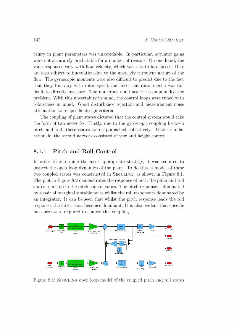
142 8. Control Strategy
tainty in plant parameters was unavoidable. In particular, actuator gainswere not accurately predictable for a number of reasons. On one hand, thevane responses vary with flow velocity, which varies with fan speed. Theyare also subject to fluctuation due to the unsteady turbulent nature of theflow. The gyroscopic moments were also difficult to predict due to the factthat they too vary with rotor speed, and also that rotor inertia was dif-ficult to directly measure. The numerous non-linearities compounded theproblem. With this uncertainty in mind, the control loops were tuned withrobustness in mind. Good disturbance rejection and measurement noiseattenuation were specific design criteria.
The coupling of plant states dictated that the control system would takethe form of two networks. Firstly, due to the gyroscopic coupling betweenpitch and roll, these states were approached collectively. Under similarrationale, the second network consisted of yaw and height control.
8.1.1 Pitch and Roll Control
In order to determine the most appropriate strategy, it was required toinspect the open loop dynamics of the plant. To do this, a model of thesetwo coupled states was constructed in Simulink, as shown in Figure 8.1.The plot in Figure 8.2 demonstrates the response of both the pitch and rollstates to a step in the pitch control vanes. The pitch response is dominatedby a pair of marginally stable poles whilst the roll response is dominated byan integrator. It can be seen that whilst the pitch response leads the rollresponse, the latter soon becomes dominant. It is also evident that specificmeasures were required to control this coupling.
Figure 8.1: Simulink open loop model of the coupled pitch and roll states

8.1. Classical Single Input-Single Output (SISO) Strategy 143
Figure 8.2: Plot of the open loop pitch and roll responses to a step in pitch
The strategy for controlling pitch and roll evolved as follows. The IMUprovides access to both absolute angles and also rates for each axis, whichallows for accurate feed-forward compensation of the gyroscopic moment.This technique utilises the measurement of rate to generate a control signal,with an appropriate gain determined by the plant parameters. It essentiallydecouples the two states, which allows the feedback compensators to betuned essentially independently.
This method was employed in the Simulink model shown in Figure 8.3,where the feed-forward and feedback compensators are highlighted. Sym-metry in the dynamics of the two states allowed the control blocks to bereplicated. Perfect cancellation of the gyroscopic moment is not possible formultiple reasons. On one hand, this would require a constant rotor speed,which is not possible. It would also require infinitely fast actuators, whichis also not the case. The method does, however, does vastly reduce theinfluence of the coupling.
The feedback compensators are proportional-derivative compensators.Integral control was not necessary due to the presence of a double integrator

144 8. Control Strategy
Figure 8.3: Simulink model of the pitch and roll controller
in the plant. The gains were tuned by firstly neglecting the gyroscopicdynamics and by inspecting the frequency response characteristics of theidealised SISO systems. The gains were then selected to provide adequatestability margins and maximum sensitivity. The plant dynamics aid thecause of robustness, as the double integrator provides for high loop gain atlow frequencies, whilst the second order servo dynamics provides good rolloff at high frequencies.
These controller gains required adjustment when they were applied tothe coupled plant model. The performance of the control system in itsentirety is shown in Figure 8.4. This response demonstrates good commandfollowing and only minor evidence of the coupling, manifest in a ripple inthe opposite state. The system also demonstrated robustness to variationsin rotor speed. A ten percent error in the rotor speed was modelled withnegligible impact on performance. Servo dynamics also had minor impact.Pole-zero cancellation blocks were experimented with, but they provided aninsignificant improvement in performance.
8.1.2 Yaw and Height ControlThe second system sought to control both yaw rate and height. It wasdecided to control yaw rate rather than yaw angle as the IMU was notcapable of providing an accurate measurement of yaw angle. This wasdue to the interference of the magnetic field of the motor with the IMUmagnetometer which is required to correct drift in the integral of the yaw
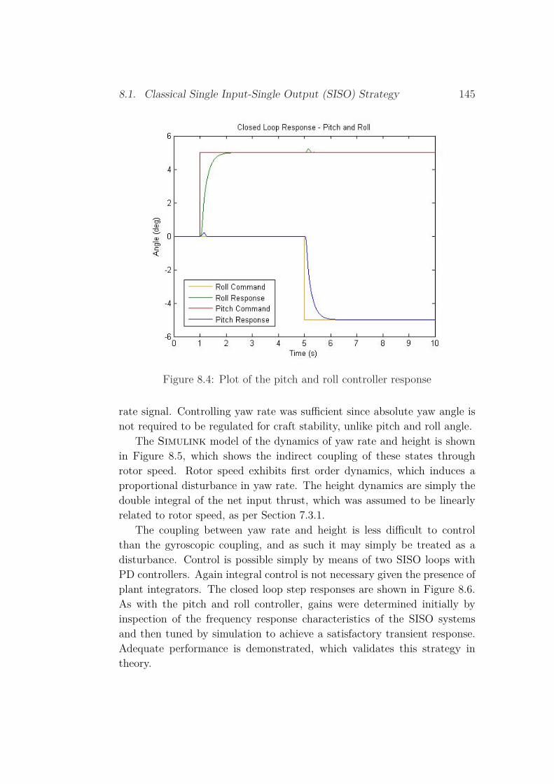
8.1. Classical Single Input-Single Output (SISO) Strategy 145
Figure 8.4: Plot of the pitch and roll controller response
rate signal. Controlling yaw rate was sufficient since absolute yaw angle isnot required to be regulated for craft stability, unlike pitch and roll angle.
The Simulink model of the dynamics of yaw rate and height is shownin Figure 8.5, which shows the indirect coupling of these states throughrotor speed. Rotor speed exhibits first order dynamics, which induces aproportional disturbance in yaw rate. The height dynamics are simply thedouble integral of the net input thrust, which was assumed to be linearlyrelated to rotor speed, as per Section 7.3.1.
The coupling between yaw rate and height is less difficult to controlthan the gyroscopic coupling, and as such it may simply be treated as adisturbance. Control is possible simply by means of two SISO loops withPD controllers. Again integral control is not necessary given the presence ofplant integrators. The closed loop step responses are shown in Figure 8.6.As with the pitch and roll controller, gains were determined initially byinspection of the frequency response characteristics of the SISO systemsand then tuned by simulation to achieve a satisfactory transient response.Adequate performance is demonstrated, which validates this strategy intheory.

146 8. Control Strategy
Figure 8.5: Simulink model of the yaw rate and height controller
8.1.3 Assessment
The preceding analysis demonstrated that a classical SISO approach to con-trol is theoretically feasible. This provided a structure upon which a con-trol system could be developed in practice. Whilst the simulation neglectedmany practical issues such as non-linearity, turbulence and measurementnoise, such issues were addressed in the implementation process.
8.2 State Space Control MethodologyIn parallel to the development of a classical controller, Dr Ben Cazzolatoconstructed a state space model of the craft, using the linearised dynamicsoutlined in Chapter 5. A state space approach to control yields a multipleinput-multiple output (MIMO) control system that is designed to accom-modate coupling between states. The following discussion describes theformulation of a suitable state space control strategy, again courtesy of DrCazzolato, and an analysis of its performance in Matlab simulation.
8.2.1 Optimal Regulator Design
In designing a state space controller, control gains are sought that placethe poles of the closed loop system in desirable locations. Pole placementcommands in Matlab toolboxes can be used to determine the requiredgains, but the method relies upon knowledge of desirable pole locations.Faster poles will always lead to better system performance, but this comes

8.2. State Space Control Methodology 147
Figure 8.6: Plot of the closed loop step response of the yaw-height controller

148 8. Control Strategy
at the cost of increased demands on the actuators and sensitivity to mea-surement noise. The optimisation between performance characteristics andcontrol effort can be solved with Linear Quadratic methods. By minimis-ing a cost function that contains penalties for both state error and controleffort, the LQ methods seek an “optimal” solution in determining feedbackgains. This method was used for the state space controller produced byCazzolato (2006).
A number of different methods are available to define the penalty ma-trices. The method used in this state model is Bryson’s method, in whichpenalties are specified as the inverse of the square of the maximum allow-able state errors. Larger gains are specified for states that are more criticalfor the stability of the craft. For instance, pitch and roll angle are allocatedlarger penalties than yaw. The advantage of applying lower control gains fora yaw error is that the actuator demands are reduced giving roll and pitchcontrol more authority over vane position. Rotor speed control performanceis limited by the capabilities of the ESC, although a slow response is de-sirable to avoid excessive demands on the yaw controller. The LQ methodtherefore provides an intuitive framework with which a regulator may bedesigned.
8.2.2 Command Tracking
After the penalty matrices were defined and the gains determined, a fullstate feedback controller was built around the plant. A command vectorwas integrated by altering the input matrix to allow tracking of non-zero setpoints. The input vector was only applied to the three orientation states andthe height, since it is not possible to for derivative states to simultaneouslytrack commands. Figure 8.7 shows the response of the roll and pitch statesto a roll angle command. Steady state error is present in the commandfollowing and thus integral control is necessary for error free tracking.
8.2.3 Integral State Feedback
Integral action was implemented by augmenting the plant with additionalstates as shown in Equation 8.1. The introduction of these states eliminatedthe steady state error in the command following of orientation and heightstates. The feedback gains on the augmented states are analogous to the
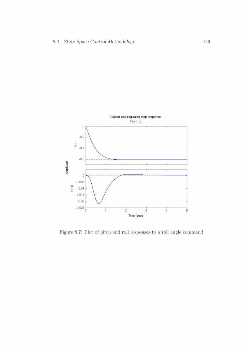
8.2. State Space Control Methodology 149
Figure 8.7: Plot of pitch and roll responses to a roll angle command

150 8. Control Strategy
integral gain used in classical compensator design, and as such they alsoprovide low frequency disturbance rejection.
xaug =
[xm
xi
]=
φ.
φ
θ.
θ
ψ.
ψ
z.z
ΩR∫(φ − φdes)dt∫(θ − θdes)dt∫(ψ − ψdes)dt∫(z − zdes)dt
(8.1)
8.2.4 Modelling Actuator DynamicsThe servo motor dynamics are modelled as a cascaded state system beforethe plant. Inputs to the actuator system are the desired servo positions, andoutputs are the actual positions, which lag the inputs in accordance with thesecond order dynamics of the motors. This rationale for this cascaded modelis that feedback of servo position is not available in the real system, so thesestates could not be included in a full state feedback controller. Modellingthe dynamics in this manner allows an assessment of the robustness of thecontroller to actuator dynamics, which were not considered in the controllerdesign. The alternative is to build a reduced order observer to estimate theactuator states.
8.2.5 Completed ModelThe full system structure as implemented in Simulink is shown pictoriallyin Figure 8.8.
The response of roll and pitch to a roll step command is shown in Fig-ure 8.9. Evidently, the augmented integral states have eliminated steady

8.2. State Space Control Methodology 151
Figure 8.8: Simulink representation of state model structure (Cazzolato,2006)
state error. The gyroscopic disturbance on the pitch rotation is also rapidlyattenuated.
Figure 8.9: Plot of the system response to a roll command in both roll andpitch states
152 8. Control Strategy
8.2.6 Assessment
The LQR state controller performs well in simulation which demonstratesthat the plant as modelled is controllable with the designed structure. Theperformance of this system in simulation is favourable over the classical con-trol structures however implementation is not possible in its current form.An estimator would be required for unmeasured states such as height androtor speed, and this is likely to alter performance. The plant model entailssubstantial uncertainty, whilst measurement noise and output disturbancesare inevitable. The robustness of this controller to these practical issues isnot proven.
This methodology is likely to be far more problematic to implement thanthe classical methodology. This is largely due to the fact that state con-trollers are difficult to tune intuitively, since it is not possible to isolate indi-vidual loops. Troubleshooting and fine tuning are likely to be very tediousand lengthy processes. As such, model uncertainty poses a serious hurdleto this approach. Given the considerable uncertainty in the system ID ofChapter 7, the classical methodology of Section 8.1 was more favourable.With this approach, individual SISO loops may be isolated and tuned se-quentially, which greatly simplifies the implementation process. Whilst thecapabilities of the control strategy posed in Section 8.1 are quite modest, itis more suited to the first iteration of control implementation.
8.2.7 Future Work
The uncertainty in the plant model dictates that if a MIMO approachis to be undertaken, design emphasis should be placed on robustness. Anumber of advanced methods have been developed for the design of robustMIMO controllers. However, the learning and development time precludedthese methods from considerations. The Linear Quadratic Gaussian (LQG)methodology is one such approach that accommodates for disturbances andmeasurement noise. Other methods, such as the H∞ method, facilitateMIMO loop shaping and robustness to model uncertainty. Both of thesemethods, however, require knowledge of the targeted noise, disturbancesand uncertainty. Subsequently, extended testing would be required in or-der to implement such methods. With ample time, the benefits of suchapproaches may be rewarding, both in system performance and academic
8.2. State Space Control Methodology 153
merit. The authors recommend that such methods are more seriously in-vestigated in the future.

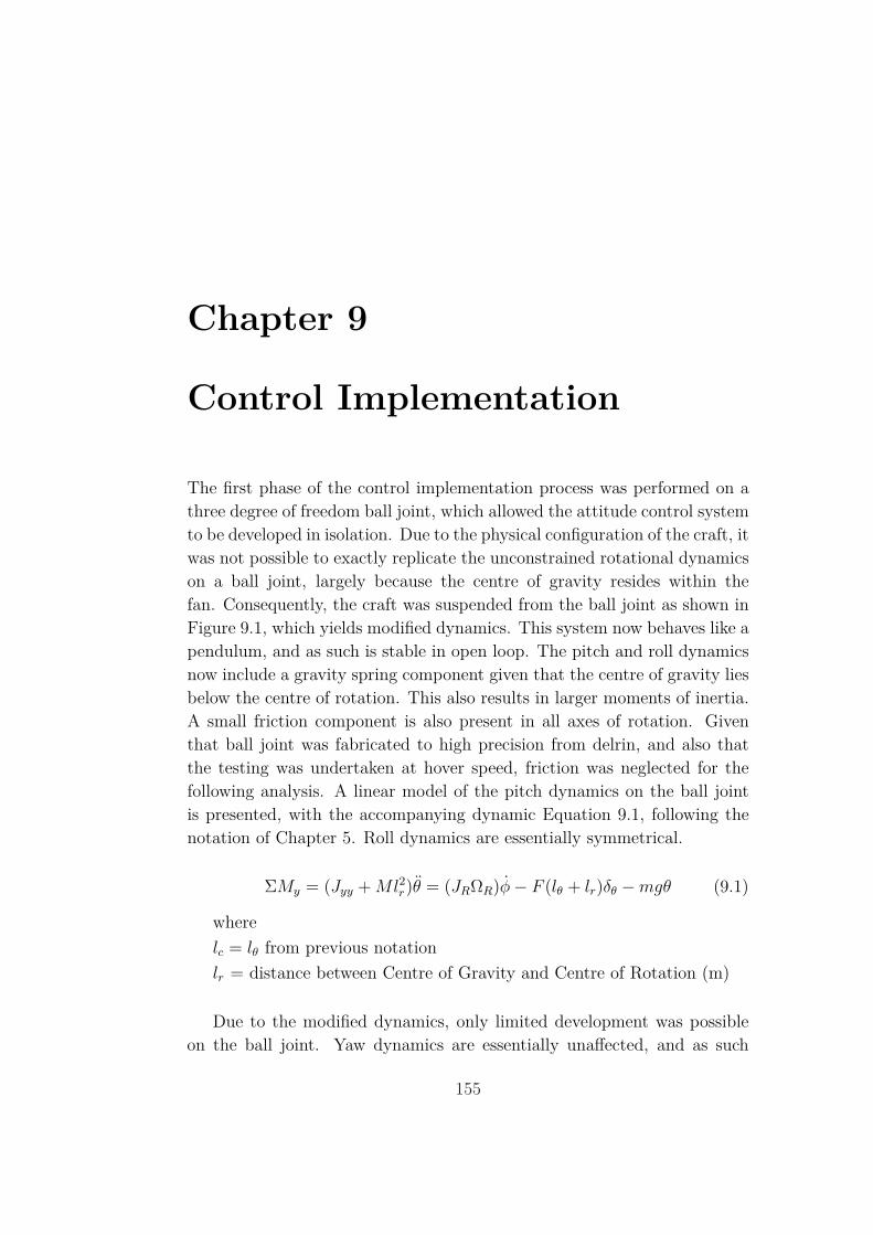
Chapter 9
Control Implementation
The first phase of the control implementation process was performed on athree degree of freedom ball joint, which allowed the attitude control systemto be developed in isolation. Due to the physical configuration of the craft, itwas not possible to exactly replicate the unconstrained rotational dynamicson a ball joint, largely because the centre of gravity resides within thefan. Consequently, the craft was suspended from the ball joint as shown inFigure 9.1, which yields modified dynamics. This system now behaves like apendulum, and as such is stable in open loop. The pitch and roll dynamicsnow include a gravity spring component given that the centre of gravity liesbelow the centre of rotation. This also results in larger moments of inertia.A small friction component is also present in all axes of rotation. Giventhat ball joint was fabricated to high precision from delrin, and also thatthe testing was undertaken at hover speed, friction was neglected for thefollowing analysis. A linear model of the pitch dynamics on the ball jointis presented, with the accompanying dynamic Equation 9.1, following thenotation of Chapter 5. Roll dynamics are essentially symmetrical.
ΣMy = (Jyy + Ml2r)θ = (JRΩR)φ − F (lθ + lr)δθ − mgθ (9.1)
wherelc = lθ from previous notationlr = distance between Centre of Gravity and Centre of Rotation (m)
Due to the modified dynamics, only limited development was possibleon the ball joint. Yaw dynamics are essentially unaffected, and as such
155
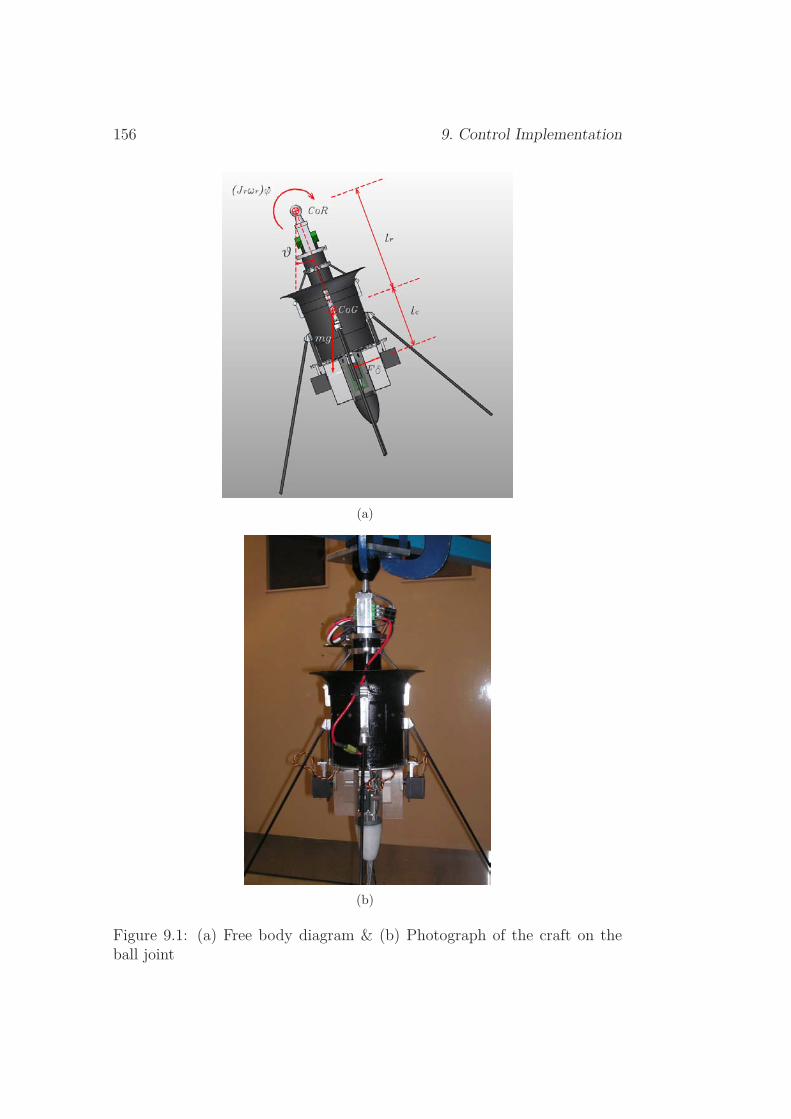
156 9. Control Implementation
(a)
(b)
Figure 9.1: (a) Free body diagram & (b) Photograph of the craft on theball joint

9.1. Yaw Rate Control 157
a valid yaw controller was able to be tuned. However, since pitch androll dynamics differed so significantly, the following approach was used toobtain valid results. Firstly, gyroscopic compensation was tuned in openloop. With appropriate scaling, this tuning is valid since the gyroscopicmoment is unaffected by the ball joint. Next, feedback gains were tunedsuch that the system was stable in this configuration. Tuning was performedfor small pitch and roll angles to minimise the influence of gravity. Thesegains were also scaled to compensate for the distorted parameters.
9.1 Yaw Rate ControlGiven that yaw rate was to be regulated, a proportional-integral controllerwas deemed adequate. Differentiation of the IMU rate data was highly noisy,and derivative control generated excessive and erratic control signals withno obvious benefit. Proportional control provided adequate disturbancerejection whilst a small integral gain was included to offset the reactivetorque induced by the rotor.
It was difficult to accurately tune the controller gains since the yaw angledata from the IMU was corrupt and the rate data contained much highfrequency noise. The proportional gain was determined largely by visualinspection of disturbance rejection performance. Integral gain was initiallytuned similarly. To fine tune the controller, a fixed period of regulated yawrate data was collected for a number of gains. The standard deviation ofthe data was computed as a quantitative measure of controller performance,as follows:
Standard Deviation
Open loop with bias 51 deg/sKp= 0.1, Ki= 0 21 deg/sKp= 0.1, Ki= 0.001 20 deg/sKp= 0.1, Ki= 0.005 19 deg/s
This rationale assumes that disturbances are random. Evidently, perfor-mance differed very little. The bottom combination was selected. Figure 9.2shows a plot of regulated yaw rate in comparison to the open loop behaviour
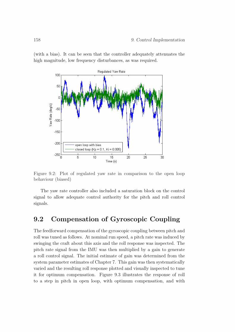
158 9. Control Implementation
(with a bias). It can be seen that the controller adequately attenuates thehigh magnitude, low frequency disturbances, as was required.
Figure 9.2: Plot of regulated yaw rate in comparison to the open loopbehaviour (biased)
The yaw rate controller also included a saturation block on the controlsignal to allow adequate control authority for the pitch and roll controlsignals.
9.2 Compensation of Gyroscopic CouplingThe feedforward compensation of the gyroscopic coupling between pitch androll was tuned as follows. At nominal run speed, a pitch rate was induced byswinging the craft about this axis and the roll response was inspected. Thepitch rate signal from the IMU was then multiplied by a gain to generatea roll control signal. The initial estimate of gain was determined from thesystem parameter estimates of Chapter 7. This gain was then systematicallyvaried and the resulting roll response plotted and visually inspected to tuneit for optimum compensation. Figure 9.3 illustrates the response of rollto a step in pitch in open loop, with optimum compensation, and with
9.2. Compensation of Gyroscopic Coupling 159
excessive compensation. The performance of the optimum compensatorattenuated the coupling to a minor ripple. This procedure was replicatedfor the orthogonal axis of rotation.
Figure 9.3: Plot of tuning roll compensation for a step in pitch
As this compensator was tuned on the ball joint, the selected gain isrequired to be scaled to account for the modified dynamics. The scalingfactor was determined as follows.
For perfect cancellation, the gyroscopic moment is in equilibrium withthe control moment.
(JRΩR)φ = F (lθ + lr)δθ (9.2)

160 9. Control Implementation
For a given roll rate, the pitch servo demand is:
δθ =(JRΩR)φ
F (lθ + lr)(9.3)
For unconstrained motion, the equivalent compensation is given by:
δ′θ =(JRΩR)φ
F lθ(9.4)
It follows that for equivalent compensation, the compensator gain shouldbe corrected by the factor:
δθ
δ′θ=
lθ + lrlθ
= 1 +lrlθ
(9.5)
9.3 Pitch and Roll Feedback Compensation
It was initially intended to tune the pitch and roll feedback compensators onthe ball joint and subsequently scale the gains to account for the modifieddynamics. Assuming perfect cancellation of the gyroscopic moment, thepitch angle transfer functions for the two configurations are:
UnconstrainedG6DOF (s) =
Θ(s)
δ(s)= − Flc
Jyys2(9.6)
PinnedG3DOF (s) =
Θ(s)
δ′(s)= − F (lc + lr)
(Jyy + ml2r) s2 + mglr(9.7)
A comparison of the (magnitude) bode plots of the two systems is shownin Figure 9.4. The poles of the pinned system are low frequency, that is,approximately 1Hz. For frequencies in excess of 1.5 Hz, the systems differonly by a small gain. However, the undamped resonance dominates theresponse of the pinned system, which precludes any transferrable tuning.This was verified to be the case in practice.
The feedback compensators for pitch and roll control are therefore re-quired to be tuned during unconstrained testing.
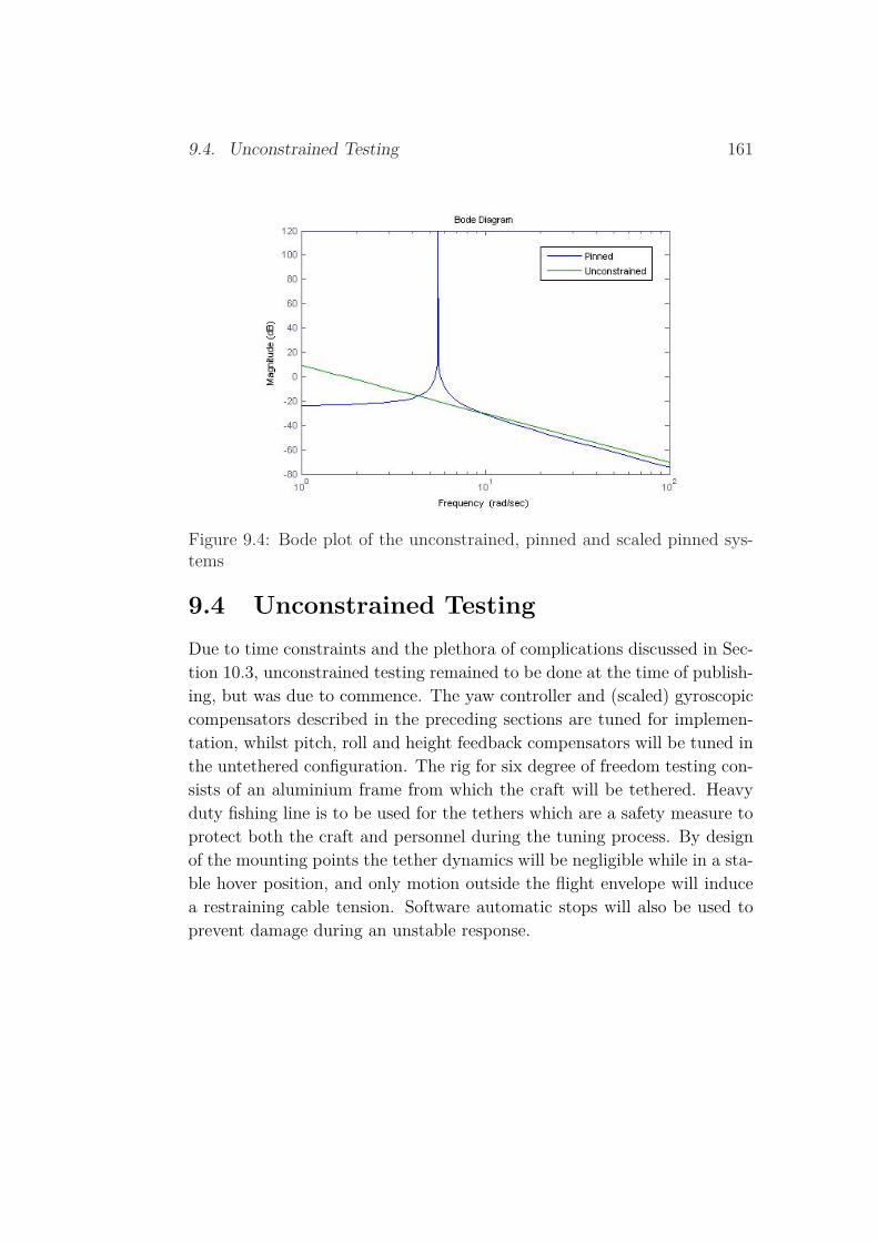
9.4. Unconstrained Testing 161
Figure 9.4: Bode plot of the unconstrained, pinned and scaled pinned sys-tems
9.4 Unconstrained TestingDue to time constraints and the plethora of complications discussed in Sec-tion 10.3, unconstrained testing remained to be done at the time of publish-ing, but was due to commence. The yaw controller and (scaled) gyroscopiccompensators described in the preceding sections are tuned for implemen-tation, whilst pitch, roll and height feedback compensators will be tuned inthe untethered configuration. The rig for six degree of freedom testing con-sists of an aluminium frame from which the craft will be tethered. Heavyduty fishing line is to be used for the tethers which are a safety measure toprotect both the craft and personnel during the tuning process. By designof the mounting points the tether dynamics will be negligible while in a sta-ble hover position, and only motion outside the flight envelope will inducea restraining cable tension. Software automatic stops will also be used toprevent damage during an unstable response.


Chapter 10
Conclusion
This chapter analyses the outcomes of the project. This includes summaris-ing the extent to which the primary and extension goals of the project weresatisfied, the breakdown of mass and cost budgets for the project, a list ofissues encountered throughout, future work to be undertaken and a post-analysis of the project.
10.1 Project Definition, Specification and Con-tract
This section reflects in retrospect on the specification and goals of the con-tract formed at the outset of the project. According to the contract for-mulated at the beginning of the project, the following specifications weregenerated:
1. The electric motor selected must be capable of generating sufficientthrust to allow control of the platform in hover. We will need to testthe thrust characteristics of the ducted fan to determine the powerrequirements for the motor.
2. Stabilization of the platform will be achieved by regulating air flowthrough 4 ducts with servo motor operated ailerons and variable guidevanes.
3. Automatic control theory will be applied to the rig and implementedon the Simulink based Quanser platform.
163

164 10. Conclusion
The project was to adhere to these specifications were applicable.This specification was based on the initial SADTU design concept. How-
ever, detailed research led to a substantial modification of the direction ofthe project. An aerodynamic analysis was conducted on the SADTU designmodel, which concluded that the concept was not viable. An alternate de-sign concept was formed which greatly simplified the task. Placing controlvanes directly in the fan efflux eliminated the requirement for control ductsand the associated thrust losses.
The primary goals for the project including the method of attainingthem is outlined, along with comments regarding their achievement:
1. Select motor to optimize thrust from fan (start of term 2).
This will involve testing the thrust characteristics of the ducted fanin order to determine the required speed and power output from theelectric motor. If they are deemed capable we will use one of the Plet-tenberg motors from last year’s VTOL project, otherwise a new motorwill be purchased.
An experiment was designed and successfully conducted to obtainthe fan characteristic. During static testing, the selected motor-fanwas proven capable of generating adequate thrust to overcome theweight of the craft. This project goal is therefore deemed to havebeen achieved on target.
2. Design platform and control ducts.
Thrust limitations will require that the platform be as light as possible.The lift/weight ratio will strongly affect the overall controllability ofthe craft and its achievement of a stable hover. Control ducts shouldbe designed to provide adequate responsiveness without compromisingthrust.
The authors feel that this goal was completed above target. Muchemphasis was placed on the mechanical design of a lightweight andstructurally sound platform which optimises controllability. The weightof the craft is less than the initial design target.

10.1. Project Definition, Specification and Contract 165
3. Formulate the mathematical equations of the dynamic system, andusing automatic control theory build Simulink and VRML basedmodels.
Our completed controller should be capable of regulating 6 DOF, al-lowing the platform to achieve a stable hover and command following.Different control strategies, both classical PID and state space, will beinvestigated.
Stable control was achieved in simulation with both classical and statespace strategies. It is noted, however, that vast scope remains fordevelopment of a more sophisticated control strategy. Significant in-vestments in time were required to implement more modern strategiessuch as those described elsewhere in this document, and such develop-ment is recommended as future work. Whilst the craft is not presentlyregulated in all six degrees of freedom, the authors feel that this goaloverall has been achieved on target.
4. Create student friendly interface.
This is in conjunction with our aim of developing the platform as ateaching aid for future students.
Using the dSPACE platform allows easy graphical user interface be-tween the model parameters and the implemented controller. Thecontrol desk program allows real time modifications and presents out-puts. This goal has been achieved on target.
The following extension goals were developed to provide an additional chal-lenge.
1. Produce a system ID of the experimental platform.
A system ID of plant parameters was not conducted not in the con-ventional sense. However, it was conducted by means of numeroustests that targeted specific system parameters. Estimates were ob-tained for all system parameters so this extension goal was achieved
166 10. Conclusion
on target. A closed loop system ID would be beneficial in obtainingmore accurate estimates of parameters such as rotor inertia howevernon-linearities, disturbances and noise may preclude valid results.
2. Onboard power, RF control.
In the process of conducting the feasibility study it was determinedthat onboard power was not possible with the Dynamax fan imple-mented in the craft. In order to achieve this goal it would be necessaryto design a larger fan with a higher thrust to power ratio. Since thiswas a major undertaking in both design and manufacture, it was notconsidered achievable in our time frame. RF control was also elimi-nated from considerations given the implicit transmission delays.
3. Advanced maneuvers.
Limitations of the controller structures used restricted the flight enve-lope to small movements about hover. A more sophisticated controlsystem is required to achieve this goal, which time constraints did notallow.
10.2 BudgetsThis section provides a summary of the mass of components utilised withinthe project along with the cost of developing the prototype.
All the way throughout the project there was an emphasis on reducingthe weight of the craft. Developing the lightest possible craft would increasethe chances of achieving stable hover. After the testing of the Dynamax fanit was decided to aim for a target craft mass of 2.5 kg. The authors had noinfluence on the mass of off-the-shelf components, however the mechanicaldesign of the chassis was considerable, whereby a final mass of 2.29 kg wasachieved. Table 10.1 summarises the mass of all components on the craft.
Since the project was not intended to have commercial appeal, the cost-ing of components was not critical. Components were selected for func-tionality, with price deciding products of similar performance. Some ofthe components used in the project were not purchased but acquired from

10.2. Budgets 167
Table 10.1: Mass budget
Component Mass (g)
Purchased components:Plettenberg 370/50/A1/S DC Motor 585Castle Creations Phoenix 110-HV ESC 135Dynamax ducted fan 240Hitec HS5475 MG digital servo motor (4×) 180ST Model RC 7.4V 1800mAh LiPo 83PicoPic microcontroller 643DM-GX1 IMU 26
Fabricated chassis:Motor & ESC mounts 147Motor/fan coupling 146Servo/control vane system 219Central hub housing 137Landing/crash systems 99Bellmouth inlet 80Duct extension 52
Auxillaries:On-board wiring & Fasteners 97
Total mass 2290
Note: The tether cables add mass with altitude @ ≈ 100 g/m
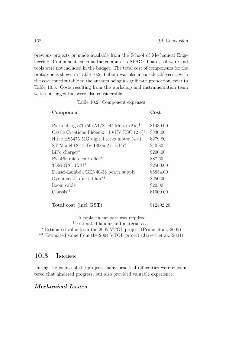
168 10. Conclusion
previous projects or made available from the School of Mechanical Engi-neering. Components such as the computer, dSPACE board, software andtools were not included in the budget. The total cost of components for theprototype is shown in Table 10.2. Labour was also a considerable cost, withthe cost contributable to the authors being a significant proportion, refer toTable 10.3. Costs resulting from the workshop and instrumentation teamwere not logged but were also considerable.
Table 10.2: Component expenses
Component Cost
Plettenberg 370/50/A1/S DC Motor (2×)† $1430.00Castle Creations Phoenix 110-HV ESC (2×)† $830.00Hitec HS5475 MG digital servo motor (4×) $279.80ST Model RC 7.4V 1800mAh LiPo* $40.80LiPo charger* $200.00PicoPic microcontroller* $87.603DM-GX1 IMU* $2500.00Densei-Lambda GEN40-38 power supply $5854.00Dynamax 5′′ ducted fan** $250.00Loom cable $20.00Chassis†† $1000.00
Total cost (incl GST) $12492.20
†A replacement part was required††Estimated labour and material cost
* Estimated value from the 2005 VTOL project (Prime et al., 2005)** Estimated value from the 2004 VTOL project (Jarrett et al., 2004)
10.3 IssuesDuring the course of the project, many practical difficulties were encoun-tered that hindered progress, but also provided valuable experience.
Mechanical Issues

10.3. Issues 169
Table 10.3: Estimated labour costs
Author Hours Salary Direct Indirect Total CostRyan Arbon 806 $20,667 $5,777 $26,867 $53,733Elias Arcondoulis 734 $18,821 $5,646 $24,467 $48,933Mark Gilmour 755 $19,359 $5,808 $25,167 $50,333Ryan Matthews 779 $19,974 $5,992 $25,967 $51,933Total 3037 $78,821 $23,646 $102,467 $204,933
Rubbing and misalignment
• During commissioning of the propulsion system, rubbing occurred be-tween the non-driven end of the rotor shaft and a static component.Fitting of the bellmouth inlet caused deformation of the fan ductwhich resulted in blade tip rubbing. Small error in strut lengths alsocaused a minor rotor misalignment. Following troubleshooting, thepropulsion system was disassembled and reassembled to rectify theseproblems.
• The first iteration servo mounting plate lacked rigidity, which led tomisalignment of the control vanes and subsequently excessive frictionloads. This system was redesigned to address this issue.
Vibration
• Excessive vibration was likely to have contributed to the ESC failure.The ESC was initially rigidly fixed to the motor, so vibration wastransmitted directly to components and soldered joints. A neoprenepad was installed between the motor and the replacement ESC.
• Vibration also contributed to measurement noise during static testing.Filtering was implemented to remove this high frequency noise.
Non-ideal vane performance
• The control vanes performed far more erratically than expected. Thiswas a consequence of both the turbulent nature of flow and also thesmall aspect ratio of the vanes. Lengthy testing was required to ac-curately estimate the mean vane response.
170 10. Conclusion
Design for Maintenance
• Throughout testing, the craft was disassembled many times for trou-bleshooting and repairs. The craft was designed for structural in-tegrity and low mass, but not ease of access or disassembly. Manyhours were spent disassembling and reassembling the craft, which mayhave been prevented with more emphasis on design for maintenance.
Power Issues
Motor Power Supply
• The large current transients produced by the mains powered DC sup-ply may have been another contributing factor in the ESC failure. Alarge power capacitor was connected in series with the power supplyto protect the replacement controller.
Servo Motor and PicoPic Power Supplies
• During the last phase of tuning on the three DOF rig, it was notedthat large servo loads (for attenuation of large disturbances) triggerederratic ESC behaviour. Investigation showed that this was a resultof the voltage drop induced by a large current draw. Initially, thePicoPic and servo motors were powered by a common LiPo battery,and the voltage drop was interfering with the PicoPic logic, whichrequires a constant voltage. This was manifest in erratic PWM signalsto the ESC. To rectify this problem, the two power supplies wereisolated, by means of an off-board DC supply. Using the peak currentload measurements from the DC supplies a more appropriate voltageregulator could be designed in future if the additional tether bulk wasproblematic, or if an untethered configuration was pursued.
Measurement Issues
Force Transducer Limitations
• The force and moment signals produced by the control vanes were atthe sensitivity limits of the six axis force transducer, resulting in small

10.3. Issues 171
signal to noise ratios. To mitigate this, aggressive filtering was usedin conjunction with slow ramp inputs.
• The transducer also had a tendency to drift, even under fixed, staticloads. Each channel required recalibration at the commencement ofeach test.
Tachometer Limitations
• The resolution of the tachometer was limited by its principle of opera-tion. As such, the accuracy of rotor speed measurements was limited.Rotor speed dynamics were particularly difficult to capture accurately.A compromise between resolution in sample time and signal resolutionwas reached.
Aliasing
• The sample frequency at which dSPACE operated caused a number ofunforeseen aliasing issues. Specifically, the tachometer required a veryhigh run speed, given the frequency of the pulse train generated. Themany filters used also required a minimum run speed. This conflictedwith the IMU software, which was limited to a relatively small sampletime. The solution was to run the IMU system as an atomic unit ata reduced frequency.
Control Issues
Non-linearities and Unmodelled Dynamics
• All simulation was conducted with a linearised model of a non-linearsystem. Thrust vectoring is highly non-linear, whilst actuator sat-uration compounds the problem. There are also other unmodelleddynamics and model uncertainties, all of which limit the validity ofsimulated results. This resulted in extended controller developmenttime on the real system. It also prevented the application of any so-phisticated control methodologies, and restricted the craft to a modestoperating envelope.
172 10. Conclusion
Yaw Angle Feedback
• The IMU estimates absolute angle by integration of the rate measure-ments produced by its gyroscopes. Drift is corrected by magnetome-ters. Given the orientation and proximity of the IMU relative to themotor, the magnetic field of the motor was corrupting the yaw an-gle measurement. This issue prevented yaw angle control, so it wasdecided to regulate yaw rate, which proved sufficient.
Height Feedback
• The Logitech Ultra-Sonic head tracker was initially intended as aheight sensor. However, it was susceptible to the excessive acousticnoise produced by the fan. An estimate of height may be producedfrom the IMU accelerometer data but this is subject to double integra-tion which results in excessive drift. The initial solution is to regulateheight rate from the IMU accelerometer with pilot-in-the-loop driftcorrection.
Radio Communication Issues
• A wireless joystick was initially intended for operator input. However,the joystick radio frequencies caused interference with the ESC, pre-venting it from operating. The joystick was replaced with an identicalhardwired unit.
• A Bluetooth link was considered to send control signals to the craft.This concept was soon abandoned due to the significant transmissiondelay associated which would severely limit control performance. Awireless link is only feasible in conjunction with embedded control.
10.4 Future WorkIf this project is to be continued in the future, the authors suggest that thefollowing work is warranted to attain stable hover. For the remainder of thesemester the authors will endeavour to:
• Develop control gains to move from the ball joint to a tethered 6 DOFconfiguration

10.4. Future Work 173
• Attach the craft to the 6 DOF tether which protects the craft fromcrash but does not restrict movement within a small working space
• Demonstrate that the craft has enough thrust to overcome its weight
• Achieve stable hover using classical control methods
However due to the time constraints imposed by the project the followingwork will not be undertaken but is proposed to increase the functionality ofthe craft. There exists two streams of future work, progressing the developedplatform or constructing a new craft based on a larger custom ducted fan.
Future work on the current platform:
• Investigation of a sensing strategy to provide closed loop translationalcontrol and expand the flight envelope of the craft. This would eitherinvolve using the Logitech ultrasonic sensor or finding a more suitablesubstitute. The acoustic noise problems experienced with the Logitechsensor may require a filtering strategy to be used on the data.
• Controller development could occur in a number of directions. Thestate space approach could be further pursued with a focus on ro-bust MIMO methods. Alternatively the classical structure could becontinued, translational data from a new sensor would allow the in-vestigation of some alternate strategies.
• A random input driven system identification could be conducted tobetter determine some of the model parameters. If a state model isprogressed then better model estimates will improve the performanceof these controllers.
The development of a custom ducted fan would require a significant amountof work. It may however allow the platform to operate fully autonomous asthe vehicle weight can increase significantly.
• Further investigation into a custom fan design with increased diam-eter relative to the Dynamax fan. As aforementioned in Section 3.3,utilising a twin-bladed propeller and designing a duct and stator vaneswill provide the best efficiency. The custom fan could also adopt anannular wing outer profile to provide lift in forward flight and housecomponents.

174 10. Conclusion
• The increase in static thrust from this custom fan would allow onboardpower. Lithium Polymer batteries are recommended to provide powersince the energy density of this type of battery is supreme. By utilisingembedded control, the use of a tether would be negated, only pilotcommands would be required by radio frequency.
• With a larger fan and onboard power, the design flight envelope couldbe expanded to allow forward flight. The aerodynamics of forwardflight should be given more consideration in both mathematical mod-elling and chassis design. The duct inlet and efflux design should alsoconsider free-stream air velocity.
• If unconstrained by a tether and moving in a large ourdoor environ-ment the ideal sensing strategy to develop would be the integrationof a GPS reciever and the existing IMU. A large body of literatureexists on such sensing combinations.
• The performance of the control vanes could be enhanced by increasingthe aspect ratio. The vanes would more likely behave as wings ratherthan deflectors.
10.5 PostanalysisReflecting on the progress of the project over the course of the year, thereis very little that the authors would do differently. The biggest threatto the success of the project was the restricted time frame and numerousdelays throughout the year continually hindered progress. Troubleshooting,particularly of electrical issues was a constant sink of available time andlong delays for the manufacture of components limited the amount of timeavailable for controller development. It was not until well after the midyear break that the final parts were received and static testing of the fullyassembled craft was possible.
A large portion of testing time was allocated to performing a detailedsystem identification, which reduced greatly the time available for controllerdevelopment. This was perhaps not the ideal scenario. Detailed design maypossibly have been pushed forward, at the expense of the concept selectionprocess. This process was vitally important to the success of the project andthis decision required much research and analysis. The initial fan testing

10.5. Postanalysis 175
was also critical, as it ensured the design of a competent propulsion system.Realistically, none of the steps taken were redundant.
The authors feel the project evolved as well as can be expected for such achallenging task. The learning curve was steep, but nonetheless stimulatingand highly satisfying.


Bibliography
AerospaceWeb. Naca 0015 lift characteristics, 2006. URLhttp://www.aerospaceweb.org. Last Accessed: May 2006.
G. Avanzini and G. Matteis. Full-envelope robust control of a shrouded-fanunmanned vehicle. Journal of Guidance Control and Dynamics, 29(2),2006.
M. Carlsson and C. Cronander. Efficient roll control using distributed con-trol surfaces and aerolastic effects. Aerospace Science and Technology, 9:143–150, 2004.
P. Castillo. Real-time stabilisation and tracking of a four-rotor mini rotor-craft. IEEE Transactions on control systems technology, 12(4), 2004.
B. Cazzolato, 2006. Personal Correspondence.
J. Craig. Introduction to robotics: mechanics and control. Pearson Educa-tion, Upper Saddle River, N.J., 2005.
CRCJA, 2006. URL http://www.crcja.org/ducted.htm. Last Accessed:May 2006.
Castle Creations, 2006. URL http://www.castlecreations.com. LastAccessed: August 2006.
VR Depo, 2006. URL http://www.vrdepot.com/vrteclg.htm. Last Ac-cessed: April 2006.
Drexel, 2006. URL www.pages.drexel.edu. Last accessed: April 2006.
Exeter, 2006. URL http://www.projects.ex.ac.uk/uav. Last accessed:April 2006.
177
178 Bibliography
J. Fleming and T. Jones. Improving control system effectiveness for ductedfan vtol uavs operating in crosswinds. American Institute of Aeronauticsand Astronautics, (AIAA-2003-6514), 2003.
Futaba, 2006. URL http://www.futaba-rc.com/servos/digitalservos.pdf.Last Accessed: May 2006.
I. Guerrero, P. Londenberg, P. Gelhausen, and A. Myklebust. A poweredlift aerodynamic analysis for the design of ducted fan uavs. AmericanInstitute of Aeronautics and Astronautics, (AIAA-2003-6567), 2003.
T. Hamel, R. Mahony, R. Lozano, and J. Ostrowski. Dynamic mod-elling and configuration stabilization for an x4-flyer. In Interna-tional Federation of Automatic Control Symposium, 2002. URLhttp://prism2.mem.drexel.edu/ billgreen/Bibliography/mahonyIFAC2002.pdf.Last accessed: April 2006.
Hitec, 2006. URL http://www.hitecrcd.com/. Last Accessed: May 2006.
Moller International, 2006. URL www.moller.com. Last accessed: April2006.
M. Jarrett, R. Ng, and T. Teske. Radio controlled vertical take-off andlanding aircraft. Master’s thesis, School of Mechanical Engineering, Uni-versity of Adelaide, 2004.
E. Johnson and M. Turbe. Modeling, control and flight testing of a smallducted fan aircraft. In AIAA Guidance, Navigation and Control Confer-ence and Exhibit, number AIAA-2005-6281, August 15-18 2005.
R. Kelso, 2006. Personal Correspondence.
B. Kuo. Automatic Control Systems. Prentice Hall, Englewood Cliffs, N.J.,1995.
K. Lim, J. Shin, D. Moerder, and E. Cooper. A new approach to atti-tude stability and control for low airspeed vehicles. American Institute ofAeronautics and Astronautics, (AIAA-2004-5008), 2004.
L. Lipera, J. Colbourne, M. Tischler, M. Mansur, M. Rotkowitz, andP. Patangui. The micro craft istar micro air vehicle: Control system

Bibliography 179
design and testing. In American Helicopter Society 57th Annual Forum,May 9-11 2001.
Microstrain, 2006. URL http://www.microstrain.com/3DMGX1.com. LastAccessed: May 2006.
M. Milam and R. Murray. A testbed for non-linear flight control techniques.In The caltech ducted fan, conference on control applications, August 22-27 1999.
Moller, 2006. URL www.moller.com. Last accessed: April 2006.
P. Moller. Robotic or remotely controlled flying platform, united statespatent, 1989. no. 4795111 B1.
B. Munson, D. Young, and T. Okiiski. Fundamentals of Fluid Mechanics.J. Wiley & Sons, Inc., 4th edition, 2002.
T. Neumann, 2004. Correspondence.
Philasae, 2006. URL www.philasae.org. Last accessed: April 2006.
Plettenberg, 2006. URL http://www.plettenberg-motoren.com/UK/index.htm.
Z. Prime, J. Sherwood, M. Smith, and A. Stabilie. Remote control verticaltake-off and landing model aircraft. Master’s thesis, School of MechanicalEngineering, University of Adelaide, 2005.
Prototypes, 2006. URL prototypes.free.fr. Last Accessed: April 2006.
R. Schlecht. Autonomous aerial vehicle - self automated dynamicthrust unit. Technical report, University of Florida, 2000. URLwww.mil.ufl.edu/publications/reu2000/SADTU.pdf. Last accessed:May 2006.
G. Schneider. Aeronautical Engineering 1. University of Adelaide, 2005.
SFU, 2006. URL www.sfu.ca/casr/101-uav2.htm. Last accessed: April2006.
TanicPacks, 2006. URL http://www.tanicpacks.com. Last Accessed: May2006.

180 Bibliography
Techsburg, 2006. URL www.techsburg.com. Last Accessed: April 2006.
J. White and J. Phelan. Stability augmentation and control decoupling forthe airborne remotely operated device. In AIAA Guidance, Navigationand Control Conference, number 87-2453, August 17-19 1991.
R. Wood, 2006. Personal Correspondence.

Appendix A
SADTU Design Analysis
In order to determine the validity of the SADTU design, an aerodynamicand incompressible flow analysis was performed on the craft’s main ductand exiting control ducts. The analysis is completely in terms of genericparameters. Deep insight was gained into the degree of pressure lossesthroughout the structure in relation to input thrust. This assisted in makinga design decision on the chosen platform employed this year.
A Cross-sectional area (m2) ε Wall roughness (m)d0 Control duct initial diameter (m) θ Radial location (rad)d1 Fan hub diameter (m) ν Dynamic viscosity (m2/s)d2 Ducted fan diameter (m) ρ Air density (kg/m3)df Control duct final diameter (m)e Control duct inlet radius (m)f Friction factorg Gravitational constant (m2/s)h Head loss (m)K Pressure loss coefficientLm Main duct length (m)Mair Molar mass of air (kg/kmol)m Mass flow rate (kg/s)~n Normal vectorP Pressure (Pa)Q Volumetric flowrate (m2/s)
181

182 A. SADTU Design Analysis
r Radius - variable (m)R Universal gas constant (J/mol/K)−→S Volumetric flowrate surfaceT Fan thrust (N)Tk Air temperature (K)u(r) Velocity profile (m/s)U Air speed (m/s)z Altitude head (m)
Assumptions
• Air is an ideal and isothermal gas (note that pressure and temperaturevalues will not be substituted into the equations).
• All of the thrust from the fan is directed to small duct and main ductthrust, refer to Figure A.1 with all losses dissipated as specified (ie,there are no unaccounted for losses)
• All losses can be attributed with a K value
• Wall roughness (ε = 5×10⁻⁶) (This is a value taken for carbon fibre -note that this value has little impact on the friction factor due to thespeed of the fluid).
• Basic propeller-momentum theory can be applied (in order to deter-mine the average output velocity from the fan based on air density,thrust generated and swept duct/propeller area).
Reynolds Number The Reynolds Number of the flow exiting the ductis required to determine the friction factor of the flow and also to determinethe flow state (ie, laminar or turbulent).
Re =UD
υ(A.1)
Using standard air conditions, υ = 1.511×10⁻⁵ m2/s, thus, Re = 3.4×10⁵

183
Figure A.1: Diagram of the control duct
Friction Factor Taking the wall thickness to be ε = 5×10⁻⁶ and knowingthat D = 0.130m,ε / D ≈ 3.9×10⁻⁵.
Using the Moody Chart, f ≈ 0.015Note that at even both extreme Reynolds numbers, the f value barely
varied.
Velocity Profile Using the velocity-thrust equation from Appendix C.2,the turbulent velocity profile is given by,
u(r) =
√2T
ρπ (d22 − d2
1)
[1 + 1.44
√f + 2.15
√flog10
(1 − 2r
D
)](A.2)
Volumetric FlowrateQ =
∫ ∫S
−→u d−→S (A.3)
whered−→S = −→n drdθ (A.4)
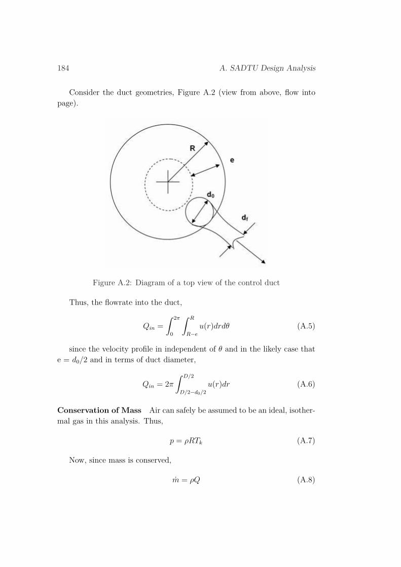
184 A. SADTU Design Analysis
Consider the duct geometries, Figure A.2 (view from above, flow intopage).
Figure A.2: Diagram of a top view of the control duct
Thus, the flowrate into the duct,
Qin =
∫ 2π
0
∫ R
R−e
u(r)drdθ (A.5)
since the velocity profile in independent of θ and in the likely case thate = d0/2 and in terms of duct diameter,
Qin = 2π
∫ D/2
D/2−d0/2
u(r)dr (A.6)
Conservation of Mass Air can safely be assumed to be an ideal, isother-mal gas in this analysis. Thus,
p = ρRTk (A.7)
Now, since mass is conserved,
m = ρQ (A.8)

185
Using ρinQin = ρoutQoutand Qav = UavA for constant, circular crosssectional areas,
Uav,out = Uav,inpind
20
poutd2f
(A.9)
Thrust per Duct (frictionless)
Tout =ρoutQ
2av,out
Aout
(A.10)
Thrust out per duct,
Tout =ρout
Aout
(ρin
ρout
)2(
2π
∫ D/2
D/2−d0/2
u(r)dr
)2
(A.11)
Since the “out” condition is the atmospheric pressure, and p is measuredin absolute, it is expected that the non-frictionless pressure drop across theduct will be small. Thus,
Tout ≈ 16πpatmMair
RTkd2f
(∫ D/2
D/2−d0/2
u(r)dr
)2
(A.12)
Thrust Losses Thrust losses through the duct can be expected from
• 90 elbow in small duct
• length of small duct
• entrance/exit effects
These losses will correspond to a pressure drop, and thus a force
Tloss =∆pπd2
f
4(A.13)
Total Duct Head Loss
hL =∑ (
KLU2
2g
)(A.14)
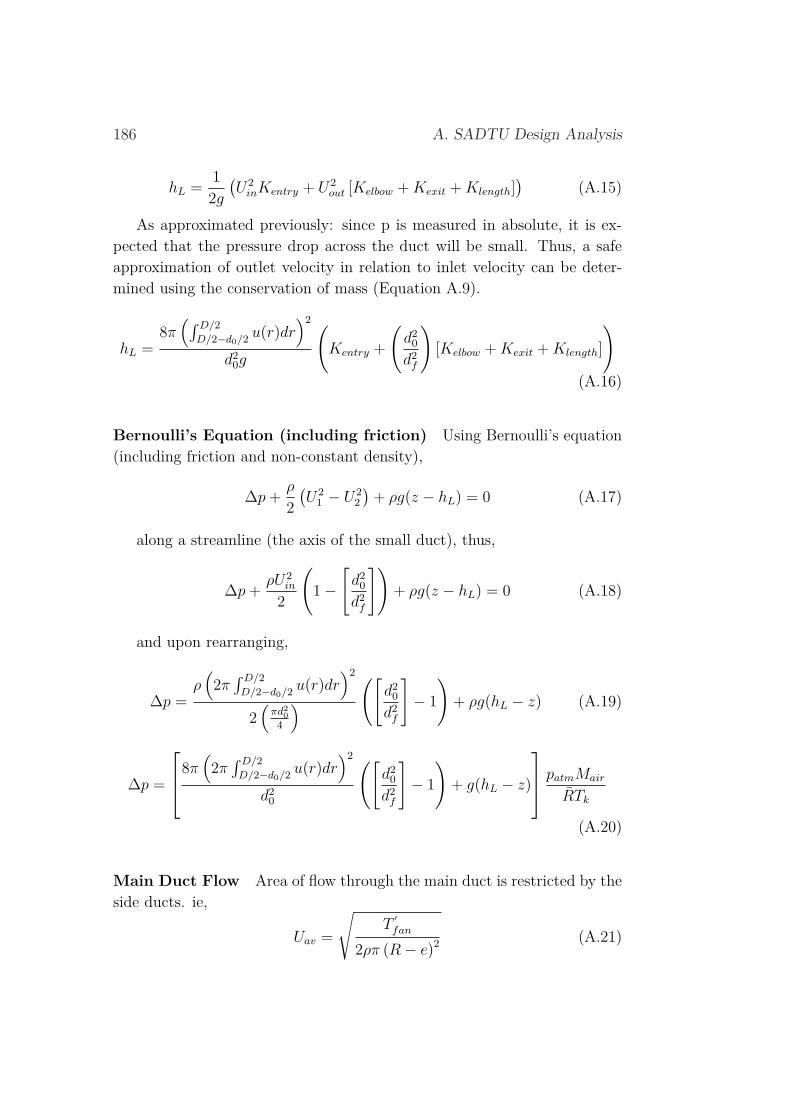
186 A. SADTU Design Analysis
hL =1
2g
(U2
inKentry + U2out [Kelbow + Kexit + Klength]
)(A.15)
As approximated previously: since p is measured in absolute, it is ex-pected that the pressure drop across the duct will be small. Thus, a safeapproximation of outlet velocity in relation to inlet velocity can be deter-mined using the conservation of mass (Equation A.9).
hL =8π
(∫ D/2
D/2−d0/2u(r)dr
)2
d20g
(Kentry +
(d2
0
d2f
)[Kelbow + Kexit + Klength]
)(A.16)
Bernoulli’s Equation (including friction) Using Bernoulli’s equation(including friction and non-constant density),
∆p +ρ
2
(U2
1 − U22
)+ ρg(z − hL) = 0 (A.17)
along a streamline (the axis of the small duct), thus,
∆p +ρU2
in
2
(1 −
[d2
0
d2f
])+ ρg(z − hL) = 0 (A.18)
and upon rearranging,
∆p =ρ
(2π
∫ D/2
D/2−d0/2u(r)dr
)2
2(
πd20
4
) ([d2
0
d2f
]− 1
)+ ρg(hL − z) (A.19)
∆p =
8π(2π
∫ D/2
D/2−d0/2u(r)dr
)2
d20
([d2
0
d2f
]− 1
)+ g(hL − z)
patmMair
RTk
(A.20)
Main Duct Flow Area of flow through the main duct is restricted by theside ducts. ie,
Uav =
√T
′fan
2ρπ (R − e)2 (A.21)
187
Thus,
Qav = (R − e)
√T
′fan
2ρ/π(A.22)
Main Duct Thrust Losses
hL =U2
av
2g
(∑K +
f∑
L
D
)(A.23)
The sources of losses in the main duct include:
• Duct length, Lm
• Change of area after small ducts
• Exit effects
Thus,
hL =
(√T
′fan
2ρπ (R − e)2
)2 (1
2g
)(K2 + K3 +
fLm
2(R − e)
)(A.24)
hL =T
′
fan
4ρπg (R − e)2
(K2 + K3 +
fLm
2(R − e)
)(A.25)
It follows,
Tloss,m =T
′
fan
4
(K2 + K3 +
fLm
2(R − e)
)(A.26)
Total Main ThrustTmain = T
′
fan − Tloss,m (A.27)
Tmain = (Tfan − 3Tduct)
[1 − 1
4
(K2 + K3 +
fLm
2(R − e)
)](A.28)


Appendix B
Dynamax Fan TestingCalculations
The following appendices outline the mathematical procedure to derivethrust from induced strain, and the derivation of the fundamental natu-ral frequency of oscillation in the beam, with an attached end mass.
B.1 Thrust/Strain Relationship
This appendix outlines the mathematics and stress analysis involved in de-termining an output thrust from a fan attached to a cantilever beam via aninduced strain in the beam. Figure B.1 outlines the testing setup and freebody diagram.
Notation The notation utilised within Section B.1 is as follows:
189

190 B. Dynamax Fan Testing Calculations
Figure B.1: Free body diagram of the Dynamax fan testing setup
b Beam width (m) ε Beam strainE Young’s modulus (Pa) ν Poisson’s ratiog Gravitational constant (m/s2) σ Bending stress (Pa)h Beam thickness (m)I Inertia of beam (mm4)md Dynamic mass (kg)ms Static mass (kg)M Bending moment (Nm)T Thrust (N)x Horizontal displacement (m)y Vertical displacement (m)
Analysis
Geometric:h 10mmb 16mmx 152mm
Material (Aluminium):
E 70x102 Pa
Mass-related:
g 9.81m/s2
ms 1.2kg
The geometric parameters were designed upon strain gauge specifica-

B.1. Thrust/Strain Relationship 191
tions and recommendations. It was recommended that the order of thestrain generated by the motor-fan combination be in the order of microstrain, which was achieved by the manipulation of the geometric parame-ters.
The bending stress in a cantilever supported beam at the point of thestrain gauge is given by:
σ =My
I(B.1)
Substituting in geometric parameters,
σ =(Tx)(h
2)
( bh3
12)
(B.2)
Thus,σ =
6Tx
bh2(B.3)
Using 2D Hooke’s Law,
εx =σx
E+ ν
σy
E(B.4)
Since there are no direct stresses in the y-direction at the point of ap-plication,
εx =σx
E(B.5)
and thus,εx =
6Tx
Ebh2(B.6)
The force used to generate strain in the gauge will include the staticmass of the fan-motor combination. In order to accommodate for this, thethrust equation is given by,
T = (ms + md)g (B.7)
Alternatively, one could ’zero’ the strain gauge, after attaching themotor-fan combo. This would still be accurate provided that ms was delib-erately set to zero. Using this,
εx =6xg(ms + md)
Ebh2(B.8)
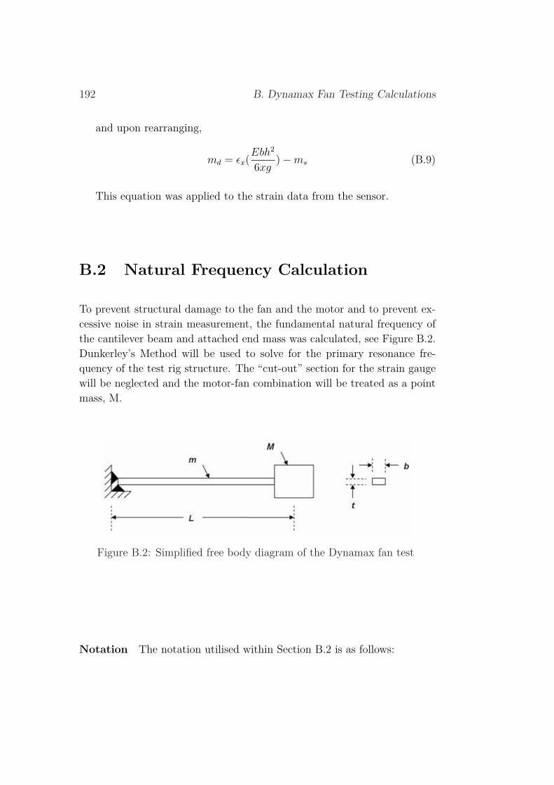
192 B. Dynamax Fan Testing Calculations
and upon rearranging,
md = εx(Ebh2
6xg) − ms (B.9)
This equation was applied to the strain data from the sensor.
B.2 Natural Frequency Calculation
To prevent structural damage to the fan and the motor and to prevent ex-cessive noise in strain measurement, the fundamental natural frequency ofthe cantilever beam and attached end mass was calculated, see Figure B.2.Dunkerley’s Method will be used to solve for the primary resonance fre-quency of the test rig structure. The “cut-out” section for the strain gaugewill be neglected and the motor-fan combination will be treated as a pointmass, M.
Figure B.2: Simplified free body diagram of the Dynamax fan test
Notation The notation utilised within Section B.2 is as follows:

B.2. Natural Frequency Calculation 193
b Beam width (m) βn Mode shape numberE Young’s modulus
(Pa)ρ Density of air
(kg/m3)I Inertia of beam
(mm4)ωb Beam natural
frequency (rad/s)L Length of beam (m) ωm Mass natural
frequency (rad/s)m Mass of beam (kg) ωT Total natural
frequency (rad/s)M Mass of motor and
fan (kg)t Beam thickness (m)
Analysis
Geometric:b 16mmt 16mmL 215 mmModal (n=1):βnL 1.87510407
Material:
ρ 2700kg/m2
E 69GPa
Mass-related:
M 1.2kg
Inertia of the beam,
I =bt3
12(B.10)
Cantilever primary resonance frequency:
ω2b = (βnL)4 EI
mL3(B.11)
Attached mass (M) natural frequency:
ω2m =
3EI
ML3(B.12)

194 B. Dynamax Fan Testing Calculations
Dunkerley’s approximation:
1
ω2T
≈ 1
ω2b
+1
ω2m
(B.13)
Using the known expressions for the beam and mass natural frequencies,
ω2T =
[mL3
(βnL)4EI+
ML3
3EI
]−1
(B.14)
Using m = ρbtL and via rearrangement,
ωT =1
2
√bt3E(βnL)4
L3(3ρbtL + M(βnL)4(B.15)
Substituting in the known parameters yields, ωT =303.36rad/s = 2,900rpm.By operating 50% outside of the resonance frequency ranges should be suf-ficient to avoid any resonance issues. Hence: 1,450rpm ≤ ωT ≤5,900rpm.

Appendix C
Air Flow Analysis
To determine the expected flow speeds and their effects on the craft dy-namics, an incompressible air analysis was performed. This includes thederivation of the duct length required for fully developed flow within thecraft and the calculation of rotor fan speed which coincides with the onsetof potential compressibility effects in the ducted fan.
C.1 CompressibilityThis appendix shows the calculation of the fan speed required to reach agiven ratio of the speed of sound, which potentially corresponds to the onsetof compressibility of air. Figure C.1 shows the model of the fan rotor andthe notation utilised.
Notation The notation utilised within Section C.1 is as follows:
c Speed of sound (m/s) ω Rotor speed (rad/s or RPM)r Radius of fan rotor (m)Uair Speed of air (m/s)v Blade tip speed (m/s)
Fan rotor and air compressibility A viscous fluid will have a no-slipboundary condition. In other words, the thin surface of air in contactwith the rotor blade area must also travel at the same speed as the rotor.
195
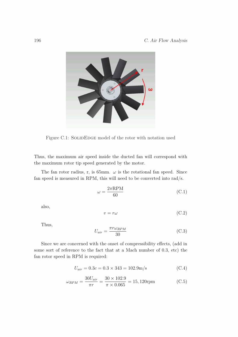
196 C. Air Flow Analysis
Figure C.1: SolidEdge model of the rotor with notation used
Thus, the maximum air speed inside the ducted fan will correspond withthe maximum rotor tip speed generated by the motor.
The fan rotor radius, r, is 65mm. ω is the rotational fan speed. Sincefan speed is measured in RPM, this will need to be converted into rad/s.
ω =2πRPM
60(C.1)
also,v = rω (C.2)
Thus,Uair =
πrωRPM
30(C.3)
Since we are concerned with the onset of compressibility effects, (add insome sort of reference to the fact that at a Mach number of 0.3, etc) thefan rotor speed in RPM is required:
Uair = 0.3c = 0.3 × 343 = 102.9m/s (C.4)
ωRPM =30Uair
πr=
30 × 102.9
π × 0.065= 15, 120rpm (C.5)

C.2. Fully Developed Flow 197
C.2 Fully Developed Flow
This appendix investigates the required duct length within the craft toachieve fully developed flow prior to reaching the control vanes. This wouldbe beneficial as it would allow for a more uniform profile onto the vanesand thus potentially increasing the control moment per vane for the sameair speed. Figure C.2 shows the model of the fan rotor and the notationutilised.
Notation The notation utilised within Section C.2 is as follows:
A Swept area (m2) µ Kinematic viscosityof air (kg/ms)
d1 Hub diameter (m) ρ Density of air(kg/m3)
d2 Rotor diameter (m) υ Dynamic viscosity ofair (m2/s)
D Duct diameter (m)L Fully developed flow
length (m)Re Reynolds numberT Thrust (N)U Velocity of air (m/s)
Fan Velocity From a given thrust value, the average velocity of air gen-erated by a ducted fan can be determined, using Equation C.6.
U =
√T
2ρA(C.6)
The swept area can be regarded as the cross sectional area of the duct,subtracted by the cross sectional area of the hub. This is shown in Fig-ure C.2.
A =π
4
(d2
2 − d21
)(C.7)

198 C. Air Flow Analysis
Thus, average velocity of air generated by the ducted fan
U =
√2T
ρπ (d22 − d2
1)(C.8)
Figure C.2: SolidEdge model of the rotor with notation used
Flow Condition The Reynolds Number of the flow exiting the duct isrequired to determine the friction factor of the flow and also to determinethe flow state (ie, laminar or turbulent).
Re =UD
υ(C.9)
Fully Developed Flow Now, the length required for fully developed flow:
L = 4.4Re16 D (C.10)
In the Ducted VTOL case,
L = 4.4
(UD
υ
) 16
D (C.11)
and since ν = µρ,
L = 4.4U16 D
76 υ− 1
6 (C.12)

C.2. Fully Developed Flow 199
Using Equation C.8,
L = 4.2D76 υ− 1
6
(T
ρ (D2 − d21)
) 112
(C.13)
Upon substitution of relevant parameters, the required length for fullydeveloped turbulent flow within the craft, L ≈ 4.6m. This is obviously fargreater than any feasible duct length able to fit within the craft.

Appendix D
Control Vane Aerodynamics
An efficient and well planned design of the control vanes for the craft isimperative for the successful controllability of the structure. The followingappendices detail the geometric design and profile generation of the controlvanes employed. In addition, a separate analysis based upon altering theexiting duct diameter for control moment optimisation.
D.1 Control Vane DesignThis appendix gives the derivation of the control force generated by eachcontrol vane, based on 2D aerodynamic theory. All assumptions and lim-itations of 2D theory are used to generate a proportionality relationshipbetween control vane force and input angle of attack.
Notation The notation utilised within Section D.1 is as follows:
Av Control vane area (m2) α Angle of attack (rad)cL Lift coefficient ρ Density of air (kg/m3)d1 Fan hub diameter (m)D Duct diameter (m)F Lift force (N)L Length (m)m Linearised lift coefficient (1/rad)
201
202 D. Control Vane Aerodynamics
t Width (m)T Thrust (N)U Velocity of air (m/s)W Thickness (m)
Assumptions
1. The incident flow field travels at uniform flow speed U (This is requiredto perform the analysis on a relatively simple level, without CFD orthin wing theory).
2. The analysis is 2-D (The duct wall to one side of the vane will helpthe 2D condition hold, as it prevents 3D wing tip effects on one sideof the wane and maintains a linear flow over the vane near the wall)
3. The lift and drag analysis can be safely based on NACA 0015 lift/dragcoefficients (The NACA 0015 is the most basic aerofoil and may un-derestimate the lift generated. The selected vane design will mostlikely be similar to this design).
4. Angles of attack will be confined to ±20 (This helps keep the controlsystem as ’linear’ as possible and allows a servo of smaller torquecapacity).
5. The exit duct has the same diameter as the ducted fan (a separateanalysis in Appendix D.2 gives an analysis of optimising the exit ductwidth for maximum control moment generation).
Analysis The force balance and geometric parameters are shown in Fig-ure D.1 and the lift/drag coefficient data in Figure D.2.
The forces acting on an aerofoil include lift and drag (provided it isstationary relative to the fluid flow). Of main concern is the lift force,which corresponds to the control force.
F =1
2ρU2AvCL (D.1)

D.1. Control Vane Design 203
Figure D.1: Diagrams of control vane forces and geometry

204 D. Control Vane Aerodynamics
Figure D.2: Diagram of the lift and drag coefficients for a NACA 0015profile (AerospaceWeb, 2006)
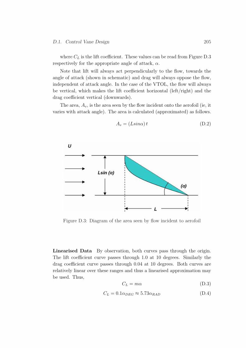
D.1. Control Vane Design 205
where CL is the lift coefficient. These values can be read from Figure D.3respectively for the appropriate angle of attack, α.
Note that lift will always act perpendicularly to the flow, towards theangle of attack (shown in schematic) and drag will always oppose the flow,independent of attack angle. In the case of the VTOL, the flow will alwaysbe vertical, which makes the lift coefficient horizontal (left/right) and thedrag coefficient vertical (downwards).
The area, Av, is the area seen by the flow incident onto the aerofoil (ie, itvaries with attack angle). The area is calculated (approximated) as follows.
Av = (Lsinα) t (D.2)
Figure D.3: Diagram of the area seen by flow incident to aerofoil
Linearised Data By observation, both curves pass through the origin.The lift coefficient curve passes through 1.0 at 10 degrees. Similarly thedrag coefficient curve passes through 0.04 at 10 degrees. Both curves arerelatively linear over these ranges and thus a linearised approximation maybe used. Thus,
CL = mα (D.3)
CL = 0.1αDEG ≈ 5.73αRAD (D.4)
206 D. Control Vane Aerodynamics
Derivation Basic 2D aerodynamic theory gives,
F =1
2ρU2AvCL (D.5)
using the derived expressions for Av and CL,
F =1
2ρLtmU2αsinα (D.6)
Using the previously derived equation between thrust and velocity fromAppendix C.2,
U =
√2T
ρπ (D2 − d21)
(D.7)
Gives the following expression in terms of fan thrust,
F =TmLtαsinα
π (D2 − d21)
(D.8)
And assuming that small angles are used, α = sin(α), the followinglinearised equation may be derived,
F =TmLtα2
π (D2 − d21)
(D.9)
And in terms of velocity, the linearised equation becomes,
F =1
2ρLtmU2α2 (D.10)
So, it can be seen that the control force (independent of various 3Deffects) has the following proportionality relation for relatively small anglesof attack,
F ∝ U2α2 (D.11)
It is expected that the 2D estimate may be twice as large as the realisticestimate, as turbulent effects, structural influences and a small aspect ratiowill inevitably decrease the lift coefficient. In addition, the aerofoil stallangle may be increased beyond the typical 18 degree limit for most NACAaerofoils.
Nonetheless, substitution of known parameters into Equation D.9 gives

D.2. Duct Width 207
a relation between control force and angle of attackT = 2.5kgm = 5.73L = 0.1mt = 0.037mD = 0.13md1= 0.065m
F ≈ 13α2 (D.12)
Control Vane Force Values: At 5 degrees:
F = 0.1N (D.13)
At 10 degrees:F = 0.4N (D.14)
At 20 degrees (control vane saturation angle):
F = 1.6N (D.15)
Actual data should be taken and then fitted to a curve (for variousconstant input thrust conditions) of the form:
F = kα2 (D.16)
where the constant, k, should be determined using fitted, empirical data.
D.2 Duct Width
It is assumed that all control vanes cover the void between the duct walland the central hub. Using this fact, an analysis was performed in orderto determine if there was a duct width that optimised the control force pervane.
Notation The notation utilised within Section D.2 is as follows:
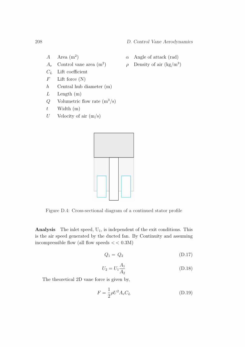
208 D. Control Vane Aerodynamics
A Area (m2) α Angle of attack (rad)Av Control vane area (m2) ρ Density of air (kg/m3)CL Lift coefficientF Lift force (N)h Central hub diameter (m)L Length (m)Q Volumetric flow rate (m3/s)t Width (m)U Velocity of air (m/s)
Figure D.4: Cross-sectional diagram of a continued stator profile
Analysis The inlet speed, U1, is independent of the exit conditions. Thisis the air speed generated by the ducted fan. By Continuity and assumingincompressible flow (all flow speeds < < 0.3M)
Q1 = Q2 (D.17)
U2 = U1A1
A2
(D.18)
The theoretical 2D vane force is given by,
F =1
2ρU2AvCL (D.19)

D.2. Duct Width 209
Figure D.5: Cross-sectional diagrams for narrowing and widening the statorprofile
And from the use of Equation D.18,
F =1
2ρ
[U1
A1
A2
]2
AvCL (D.20)
Since ρ and CL are independent of geometry,
F ∝[U1
A1
A2
]Av (D.21)
Also, (see Appendix D.1)
Av = Ltsin (α) (D.22)
Since this analysis is concerned with geometry, alpha is constant for bothanalyses. It is also assumed in both cases the vanes have equal length. So, Av ∝ t,
F ∝ U21 t
A21
A22
(D.23)
Note that U1 and A1 are fixed parameters (properties of the ducted fan).Thus they may be held constant. Also,
A2 =π
4(2t + h)2 (D.24)

210 D. Control Vane Aerodynamics
Hence,F ∝ t
(2t + h)2 (D.25)
Using a hub diameter of 55mm, an optimised control vane width plotwas generated. This is shown in Figure D.6.
Figure D.6: Plot of control vane width optimisation (2D Theory)
D.3 NACA 0015 Profile GenerationThe profile of the aerofoil is governed by a NACA equation, which deter-mines the width of the aerofoil relative to its length. This determines thelift and drag characteristics of the vane. The design of the control vane andimplementation in SolidEdge is given in this Appendix.
All symmetric NACA aerofoil profiles are governed by the followingequation:
y(x) = 5t(0.2969√
x − 0.126x − 0.3516x2 + 0.2843x3 − 0.1015x4) (D.26)
In addition, the numbers used in the aerofoil profile represent the valueused for t in the governing equation. In the case of the craft control vanes,NACA 0015 was used. Thus, the corresponding value for t = 0.15. Notethat all values of x, y and t are dimensionless. They are only used to give

D.3. NACA 0015 Profile Generation 211
the overall relationship between width and length. This equation was inputinto Matlab with the resulting plot shown in Figure D.7.
Figure D.7: Plot of aerofoil curvature
From Appendix D.1, a required control vane length was determined.From this, the non-dimensionalised length was converted into an actuallength (100mm) and thus, a series of actual data points of the profile couldbe dimensionalised and input into SolidEdge. A spline was fitted to theresulting points and then mirrored about the central axis. Both ends wererounded (by adding a fillet). The result is shown in Figure D.8.
Figure D.8: SolidEdge data points forming the control vane profile
From the resulting analysis in Appendix D.1, a resulting vane widthwas determined. The profile shown in Figure D.8 was extruded out to this

212 D. Control Vane Aerodynamics
width (37mm). In addition, holes were cut out the profile in order to fit anaxle and a mount for the servo motor connection. The result is shown inFigure D.9.
Figure D.9: SolidEdge model of the control vanes

Appendix E
Bellmouth Inlet Optimisation
To increase the thrust efficiency of the overall craft, a bellmouth inlet wasdesigned. It was later analysed to determine optimal geometries and themagnitude of the net thrust benefit. The incompressible flow analysis is de-scribed and depicted in optimisation plots. This analysis is based upon theoptimisation of inlet pressure losses with associated increase of bellmouthmass.
Notation The notation utilised in this appendix is defined as follows:
A Cross-sectional area (m2) ρ Density of air (kg/m3)D Duct diameter (m)h Central hub diameter (m)K Pressure loss coefficient.m Air mass flow rate (kg/s)∆P Pressure Drop (Pa)T Thrust (N)U Air speed (m/s)
Inlet Losses The inlet loss coefficient, K, is related to the ratio of inletradius of curvature to inlet diameter (Munson et al., 2002). This is depictedin Figure E.1 and numerically in Table E.1.
Pressure losses are proportional to the loss coefficient, K, and also pro-
213
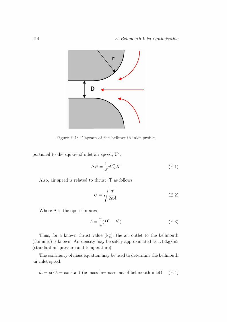
214 E. Bellmouth Inlet Optimisation
Figure E.1: Diagram of the bellmouth inlet profile
portional to the square of inlet air speed, U2.
∆P =1
2ρU2
inK (E.1)
Also, air speed is related to thrust, T as follows:
U =
√T
2ρA(E.2)
Where A is the open fan area
A =π
4(D2 − h2) (E.3)
Thus, for a known thrust value (kg), the air outlet to the bellmouth(fan inlet) is known. Air density may be safely approximated as 1.13kg/m3(standard air pressure and temperature).
The continuity of mass equation may be used to determine the bellmouthair inlet speed.
.m = ρUA = constant (ie mass in=mass out of bellmouth inlet) (E.4)

215
Table E.1: Inlet loss coefficients: Left, dimensionless & Right, D = 0.13m(Munson et al., 2002)
r/D K0 0.5
0.04 0.250.08 0.130.12 0.10.15 0.070.19 0.040.23 0.030.27 0.020.31 0.020.38 0.020.54 0.010.77 0.011.54 0.01
r (mm) K0 0.55 0.2510 0.1315 0.120 0.0725 0.0430 0.0335 0.0240 0.0250 0.0270 0.01100 0.01200 0.01
Since compressibility effects may be ignored (all inlet flows exiting thebellmouth are significantly less than 0.3M = 103m/s), this may be furtherreduced to:
Uin = Uout(Aout
Ain
) (E.5)
This gives the air speed at the inlet of the bellmouth.The thrust benefit of the bellmouth may be determined as:
T = ∆PAout (E.6)
The results are tabulated for a craft thrust = 2.5kg (fan speed ≈ 15,500rpm)
Mass Increase As the inlet pressure loss coefficient increases with in-creasing bellmouth radius, so too does its mass. The respective masseswere determined using SolidEdge and inputting an appropriate densityvalue for each.
Optimisation Comparing the mass benefit with the structure mass atvarious craft thrusts:
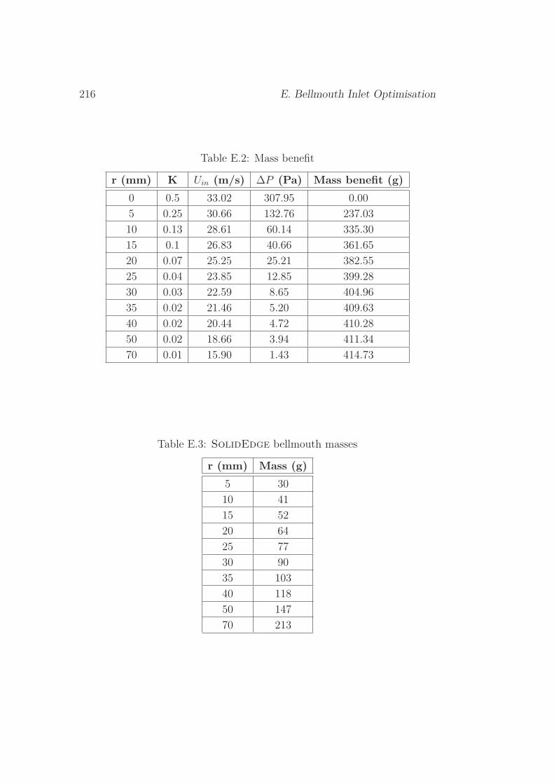
216 E. Bellmouth Inlet Optimisation
Table E.2: Mass benefit
r (mm) K Uin (m/s) ∆P (Pa) Mass benefit (g)0 0.5 33.02 307.95 0.005 0.25 30.66 132.76 237.0310 0.13 28.61 60.14 335.3015 0.1 26.83 40.66 361.6520 0.07 25.25 25.21 382.5525 0.04 23.85 12.85 399.2830 0.03 22.59 8.65 404.9635 0.02 21.46 5.20 409.6340 0.02 20.44 4.72 410.2850 0.02 18.66 3.94 411.3470 0.01 15.90 1.43 414.73
Table E.3: SolidEdge bellmouth masses
r (mm) Mass (g)5 3010 4115 5220 6425 7730 9035 10340 11850 14770 213

217
Table E.4: Net mass budget
Net mass benefit (g)r (mm) 1 kg 2 kg 3 kg 4 kg 5 kg
0 0 0 0 0 05 64.81 159.63 207.03 254.44 349.2510 93.12 227.24 294.30 361.36 495.4715 92.66 237.32 309.65 381.98 526.6520 89.02 242.04 318.55 395.07 548.0925 82.71 242.42 322.28 402.14 561.8530 71.99 233.97 314.96 395.96 557.9435 60.85 224.70 306.63 388.55 552.4040 46.11 210.22 292.28 374.34 538.4550 17.54 182.07 264.34 346.61 551.1570 — 118.79 201.73 284.68 450.58
This is displayed graphically:
Figure E.2: Bellmouth optimisation plot