ARTICLE IN PRESS

0925-2312/$ - se

doi:10.1016/j.ne

�CorrespondE-mail addr

zhaodeli@sjtu.o

Neurocomputing 70 (2007) 1547–1553

www.elsevier.com/locate/neucom

Letters

Linear local tangent space alignment and application to face recognition

Tianhao Zhang�, Jie Yang, Deli Zhao, Xinliang Ge

Institute of Image Processing and Pattern Recognition, Shanghai Jiao Tong University, P.O. Box A0503221, 800 Dongchuan Road, Shanghai 200240, China

Received 18 March 2006; received in revised form 18 November 2006; accepted 20 November 2006

Communicated by M. Welling

Available online 12 December 2006

Abstract

In this paper, linear local tangent space alignment (LLTSA), as a novel linear dimensionality reduction algorithm, is proposed. It uses

the tangent space in the neighborhood of a data point to represent the local geometry, and then aligns those local tangent spaces in the

low-dimensional space which is linearly mapped from the raw high-dimensional space. Since images of faces often belong to a manifold

of intrinsically low dimension, we develop LLTSA algorithm for effective face manifold learning and recognition. Comprehensive

comparisons and extensive experiments show that LLTSA achieves much higher recognition rates than a few competing methods.

r 2007 Elsevier B.V. All rights reserved.

Keywords: Manifold learning; Dimensionality reduction; Linear local tangent space alignment (LLTSA); Face recognition

1. Introduction

The goal of dimensionality reduction is to discover thehidden structure from the raw data automatically. This isalso the key issue in unsupervised learning. There are manyclassical approaches for dimensionality reduction such asprincipal component analysis (PCA) [9], multidimensionalscaling (MDS) [4], and independent component analysis(ICA) [3]. All of these methods are easy to implement andexploited popularly. Unfortunately, they fail to discoverthe underlying nonlinear structure as traditional linearmethods. Recently, more and more nonlinear techniquesbased manifold learning have been proposed. The repre-sentative spectral methods are Isomap [16], locally linearembedding (LLE) [13], Laplacian Eigenmap (LE) [2], localtangent space alignment (LTSA) [17], etc. These nonlinearmethods aim to preserve local structures in small neighbor-hoods and successfully derive the intrinsic features ofnonlinear manifolds. However, they are implementedrestrictedly on the training sets and cannot show explicitmaps on new testing data points for recognition problems.To overcome the drawback, He et al. [5] proposed a

e front matter r 2007 Elsevier B.V. All rights reserved.

ucom.2006.11.007

ing author. Tel.: +8621 34204035.

esses: zhangtianhao@sjtu.edu.cn (T. Zhang),

rg (D. Zhao).

method named locality preserving projection (LPP) toapproximate the eigenfunctions of the Laplace–Beltramioperator on the manifold and the new testing pointscan be mapped to the learned subspace without trouble.LPP is a landmark of linear algorithms based manifoldlearning.In this paper, inspired by the idea of LTSA [17], we

propose a novel linear dimensionality reduction algorithm,called linear local tangent space alignment (LLTSA). Ituses the tangent space in the neighborhood of a data pointto represent the local geometry, and then aligns those localtangent spaces in the low-dimensional space which islinearly mapped from the raw high-dimensional space. Themethod can be viewed as a linear approximation of thenonlinear local tangent space alignment [17] algorithm andthe technique of linearization is similar to the fashion ofLPP [5]. Since images of faces, represented as high-dimensional pixel arrays, often belong to a manifold ofintrinsically low dimension [14], we develop LLTSAalgorithm for effective face manifold learning and recogni-tion. Comprehensive comparisons and extensive experi-ments show that LLTSA achieves much higher recognitionrates than a few competing methods.The rest of the paper is organized as follows: LLTSA

algorithm is described concretely in Section 2. In Section 3,several experiments are carried out to evaluate our LLTSA

ARTICLE IN PRESST. Zhang et al. / Neurocomputing 70 (2007) 1547–15531548

algorithm and the experimental results are presented.Finally, the conclusions are given in Section 4.

2. Linear local tangent space alignment

2.1. Manifold learning via linear dimensionality reduction

Consider a data set X ¼ ½x1; . . . ;xN � sampled with noisefrom Md which is an underlying nonlinear manifold ofdimension d. Furthermore, suppose Md is embedded in theambient Euclidean space Rm, where dom. The problemthat our algorithm solves is to find a transformation matrixA that maps the set X of N points to the set Y ¼

½y1; . . . ; yN � in Rd, such that Y ¼ ATXHN , where HN ¼

I � eeT=N represents the centering matrix, I is the identitymatrix, and e is an N-dimensional column vector of allones.

2.2. The algorithm

Given the data set X ¼ ½x1; . . . ;xN � in Rm, for each pointxi, we denote the set of its k nearest neighbors by a matrixX i ¼ ½xi1 ; . . . ;xik

�. To preserve the local structure of eachXi, we should compute the local linear approximation forthe data points in Xi using tangent space [17]. We have

arg minx;Y;Q

Xk

j¼1

xij� ðxþQyjÞ

�� ��22¼ arg min

Y;QX iHk �QY�� ��2

2,

(1)

where Hk ¼ I � eeT=k, Q is an orthonormal basis matrixof the tangent space and has d columns, andY ¼ ½y1; . . . ; yk�, where yj is the local coordinate corre-sponding to the basis Q. The optimal x in the aboveoptimization is given by xi, the mean of all the xij

s and theoptimal Q is given by Qi, the matrix of d left singularvectors of XiHk corresponding to its d largest singularvalues, and Y is given by Yi defined as

Yi ¼ QTi X iHk ¼ ½y

ðiÞ1 ; . . . ; y

ðiÞk �; yðiÞj ¼ QT

i ðxij� xiÞ. (2)

Note that, the algorithm just mentioned essentially per-forms a local principal component analysis; the ys are theprojections of the points in a local neighborhood on thelocal PCA.

Now, we can construct [17] the global coordinates yi,i ¼ 1; . . . ;N, in Rd based on the local coordinate yðiÞj , whichrepresents the local geometry,

yij¼ yi þ Liy

ðiÞj þ �

ðiÞj ; j ¼ 1; . . . ; k; i ¼ 1; . . . ;N, (3)

where yi is the mean of yijs, Li is a local affine

transformation matrix that needs to be determined, and�ðiÞj the local reconstruction error. Let Y i ¼ ½yi1

; . . . ; yik� and

Ei ¼ ½�ðiÞ1 ; . . . ; �

ðiÞk �, we have

Y iHk ¼ LiYi þ Ei. (4)

To preserve as much of the local geometry in the low-dimensional feature space, we intend to find yi and Li to

minimize the reconstruction errors �ðiÞj , i.e.,

argminY i ;Li

Xi

Eik k22 � argmin

Y i ;Li

Xi

Y iHk � LiYik k22. (5)

Therefore, the optimal affine transformation matrix Li hasthe form Li ¼ Y iHkY

þi , and Ei ¼ Y iHkðI �Yþi YiÞ, where

Yþi is the Moore–Penrose generalized inverse of Yi.Let Y ¼ ½y1; . . . ; yN � and Si be the 0–1 selection matrix

such that YSi ¼ Y i. The objective function is converted tothis form

arg minY

Xi

Eik k2F ¼ arg min

YYSWk k2F

¼ arg minY

trðYSWWTSTYTÞ, ð6Þ

where S ¼ ½S1; . . . ;SN �, and W ¼ diagðW 1; . . . ;W N Þ withW i ¼ HkðI �Yþi YiÞ. Note that, according to the numer-ical analysis in [17], Wi can also be written as

W i ¼ HkðI � V iVTi Þ, (7)

where Vi is the matrix of d right singular vectors of XiHK

corresponding to its d largest singular values. To uniquelydetermine Y, we impose the constraint YYT

¼ Id. Finally,considering the map Y ¼ ATXHN , the objective functionhas the ultimate form

arg minY

trðATXHNBHNXTAÞ;

ATXHNXTA ¼ Id ;

8<: (8)

where B ¼ SWWTST. It is easily shown that the aboveminimization problem can be converted to solving ageneralized eigenvalue problem as follows:

XHNBHNXTa ¼ lXHNXTa. (9)

Let the column vectors a1; a2; . . . ; ad be the solutions ofEq. (9), ordered according to the eigenvalues, l1ol2o � � �old . Thus, the transformation matrix A which minimizesthe objective function is as follows:

A ¼ ða1; a2; . . . ; adÞ. (10)

In the practical problems, one often encounters thedifficulty that XHNXT is singular. This stems from the factthat the number of data points is much smaller than thedimension of the data. To attack the singularity problem ofXHNXT, we use the PCA [1,6] to project the data set to theprincipal subspace. In addition, the preprocessing usingPCA can reduce the noise.According to above preparation, we now summarize the

Linear Local Tangent Space Alignment algorithm, there-into, steps 3 and step 4 are similar to the correspondingalgorithm steps in [17], where we can get the comprehensivereference.Given a data set X ¼ ½x1; . . . ;xN �.Step 1: PCA projection. Project the data set X into the

PCA subspace by throwing away the minor components.To make it clear, we still use X to denote the data set in thePCA subspace in the following steps. We denote by APCA

the transformation matrix of PCA.

ARTICLE IN PRESST. Zhang et al. / Neurocomputing 70 (2007) 1547–1553 1549

Step 2: Determining the neighborhood. For each xi,i ¼ 1; . . . ;N, determine the k nearest neighbors xij

of xi,j ¼ 1; . . . ; k.

Step 3. Extracting local information. Compute Vi, thematrix of d right singular vectors of XiHK corresponding toits d largest singular values., and set W i ¼ HkðI � ViV

Ti Þ.

Step 4. Constructing alignment matrix. Form the matrixB by locally summing as follows:

BðI i; I iÞ BðI i; I iÞ þW iWTi ; i ¼ 1; . . . ;N (11)

with the initialization B ¼ 0, where I i ¼ fi1; . . . ; ikg denotesthe set of indices for the k nearest neighbors of xi.

Step 5. Computing the maps. Compute the eigenvectorsand eigenvalues for the generalized eigenvalue problem

XHNBHNXTa ¼ lXHNXTa. (12)

Then we have the solutions a1; a2 . . . ; ad ordered accord-ing to the eigenvalues, l1ol2o � � �old , and we haveALLTSA ¼ ða1; a2; . . . ; ad Þ. Therefore, the ultimate transfor-mation matrix is as follows: A ¼ APCAALLTSA, andX ! Y ¼ ATXHN .

3. Experiments

In this section, several experiments are carried out toevaluate our proposed LLTSA algorithm. We begin withtwo synthetic examples to show the effectiveness of ourmethod.

Fig. 1. 2000 random points sampled on the synthetic data. (a) Random

points on swiss roll, (b) random points on S-curve.

Fig. 2. Results of four methods applied to Swissr

Fig. 3. Results of four methods applied to S-cur

3.1. Synthetic example

The Swissroll and the S-curve [13], two well-knownsynthetic data sets, are exploited in the experiment. Fig. 1shows the 2000 random data sampled on the Swissroll andthe S-curve which are used for training. Different from thestyle of nonlinear methods [17], we can evaluate othernovel 2000 random data by the projection which is learnedon the training data. Figs. 2 and 3 show the resultsobtained by PCA, LPP , NPE (linearized version ofLLE) [7] and LLTSA in the two data sets. Note that wecarry out our LLTSA algorithm without the PCAprojection step since the computational problem ofeigenanalysis pointed out in Section 2 does not appear.As can be seen, LLTSA together with NPE can preservethe local geometric structure well, whereas PCA and LPPfail to do so.

3.2. Face recognition

A face recognition task can be viewed as a multi-classclassification problem. First, we carry out our LLTSAalgorithm on the training face images and learn thetransformation matrix. Second, each test face image ismapped into a low-dimensional subspace via the transfor-mation matrix. Finally, we classify the test images by thenearest neighbor classifier.We compare our proposed LLTSA algorithm with

baseline, PCA, LPP, NPE [7] and the original LTSA usingthe publicly available databases: ORL [12], AR [11], andPIE [15]. For the baseline method, the recognition is simplyperformed in the input space without dimensionalityreduction; For the LPP method and the NPE method,the tests are implemented by the unsupervised way. For theoriginal LTSA method, we use a simple interpolationscheme described in [10] to map testing points. For all theexperiments, the images are cropped based on the centersof eyes, and the cropped images are normalized to the

oll. (a) PCA, (b) LPP, (c) NPE, (d) LLTSA.

ve. (a) PCA, (b) LPP, (c) NPE, (d) LLTSA.

ARTICLE IN PRESS

Table 1

Best recognition rate (%) of six methods on the ORL database

Method 3 Train 5 Train

T. Zhang et al. / Neurocomputing 70 (2007) 1547–15531550

32� 32 pixel arrays and with 256 gray levels per pixel. Weuse the preprocessed versions of the ORL database and thePIE database which are publicly available from X. He’ webpage [8]. The images of the AR database are preprocessedby ourselves.

3.2.1. ORL

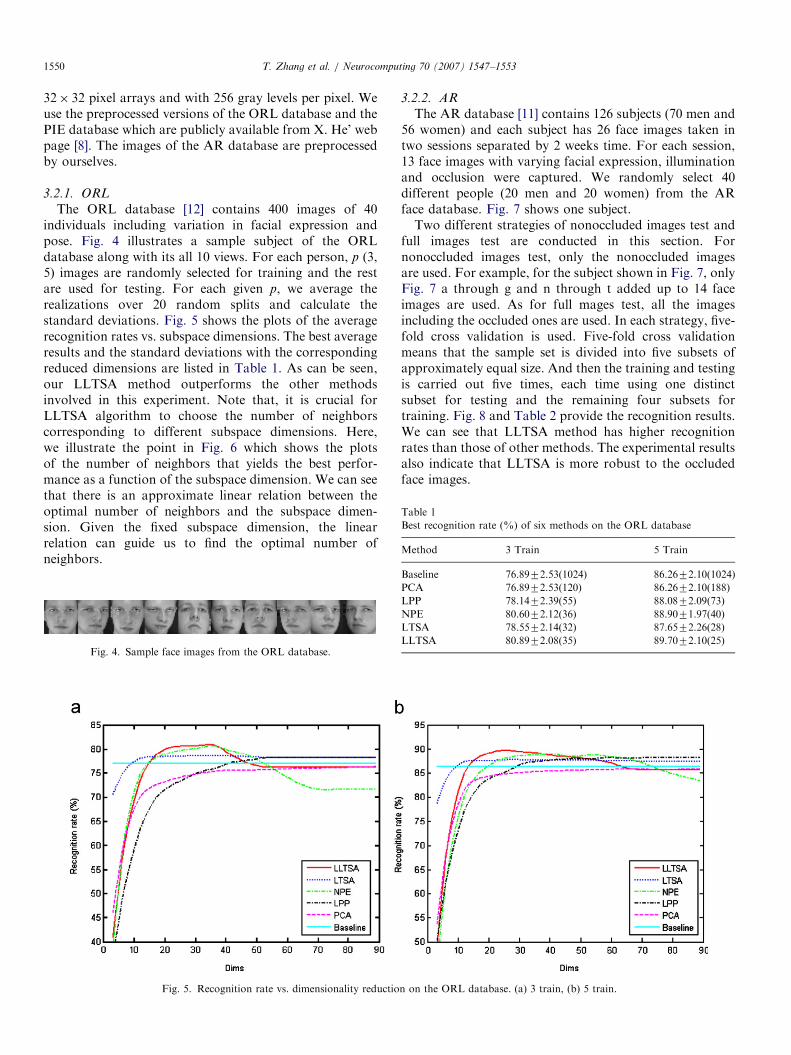
The ORL database [12] contains 400 images of 40individuals including variation in facial expression andpose. Fig. 4 illustrates a sample subject of the ORLdatabase along with its all 10 views. For each person, p (3,5) images are randomly selected for training and the restare used for testing. For each given p, we average therealizations over 20 random splits and calculate thestandard deviations. Fig. 5 shows the plots of the averagerecognition rates vs. subspace dimensions. The best averageresults and the standard deviations with the correspondingreduced dimensions are listed in Table 1. As can be seen,our LLTSA method outperforms the other methodsinvolved in this experiment. Note that, it is crucial forLLTSA algorithm to choose the number of neighborscorresponding to different subspace dimensions. Here,we illustrate the point in Fig. 6 which shows the plotsof the number of neighbors that yields the best perfor-mance as a function of the subspace dimension. We can seethat there is an approximate linear relation between theoptimal number of neighbors and the subspace dimen-sion. Given the fixed subspace dimension, the linearrelation can guide us to find the optimal number ofneighbors.

Fig. 4. Sample face images from the ORL database.

Fig. 5. Recognition rate vs. dimensionality reductio

3.2.2. AR

The AR database [11] contains 126 subjects (70 men and56 women) and each subject has 26 face images taken intwo sessions separated by 2 weeks time. For each session,13 face images with varying facial expression, illuminationand occlusion were captured. We randomly select 40different people (20 men and 20 women) from the ARface database. Fig. 7 shows one subject.Two different strategies of nonoccluded images test and

full images test are conducted in this section. Fornonoccluded images test, only the nonoccluded imagesare used. For example, for the subject shown in Fig. 7, onlyFig. 7 a through g and n through t added up to 14 faceimages are used. As for full mages test, all the imagesincluding the occluded ones are used. In each strategy, five-fold cross validation is used. Five-fold cross validationmeans that the sample set is divided into five subsets ofapproximately equal size. And then the training and testingis carried out five times, each time using one distinctsubset for testing and the remaining four subsets fortraining. Fig. 8 and Table 2 provide the recognition results.We can see that LLTSA method has higher recognitionrates than those of other methods. The experimental resultsalso indicate that LLTSA is more robust to the occludedface images.

n on the ORL database. (a) 3 train, (b) 5 train.

Baseline 76.8972.53(1024) 86.2672.10(1024)

PCA 76.8972.53(120) 86.2672.10(188)

LPP 78.1472.39(55) 88.0872.09(73)

NPE 80.6072.12(36) 88.9071.97(40)

LTSA 78.5572.14(32) 87.6572.26(28)

LLTSA 80.8972.08(35) 89.7072.10(25)

ARTICLE IN PRESS

Fig. 6. Number of neighbors vs. dimensionality reduction on the ORL database. (a) 3 train, (b) 5 train.

Fig. 7. Sample face images from the AR database. On the first row are images recorded in the first session, on the second row are recorded in the second

session.

Fig. 8. Recognition rate vs. dimensionality reduction on the AR database. (a) Nonoccluded images test, (b) full images test.

T. Zhang et al. / Neurocomputing 70 (2007) 1547–1553 1551

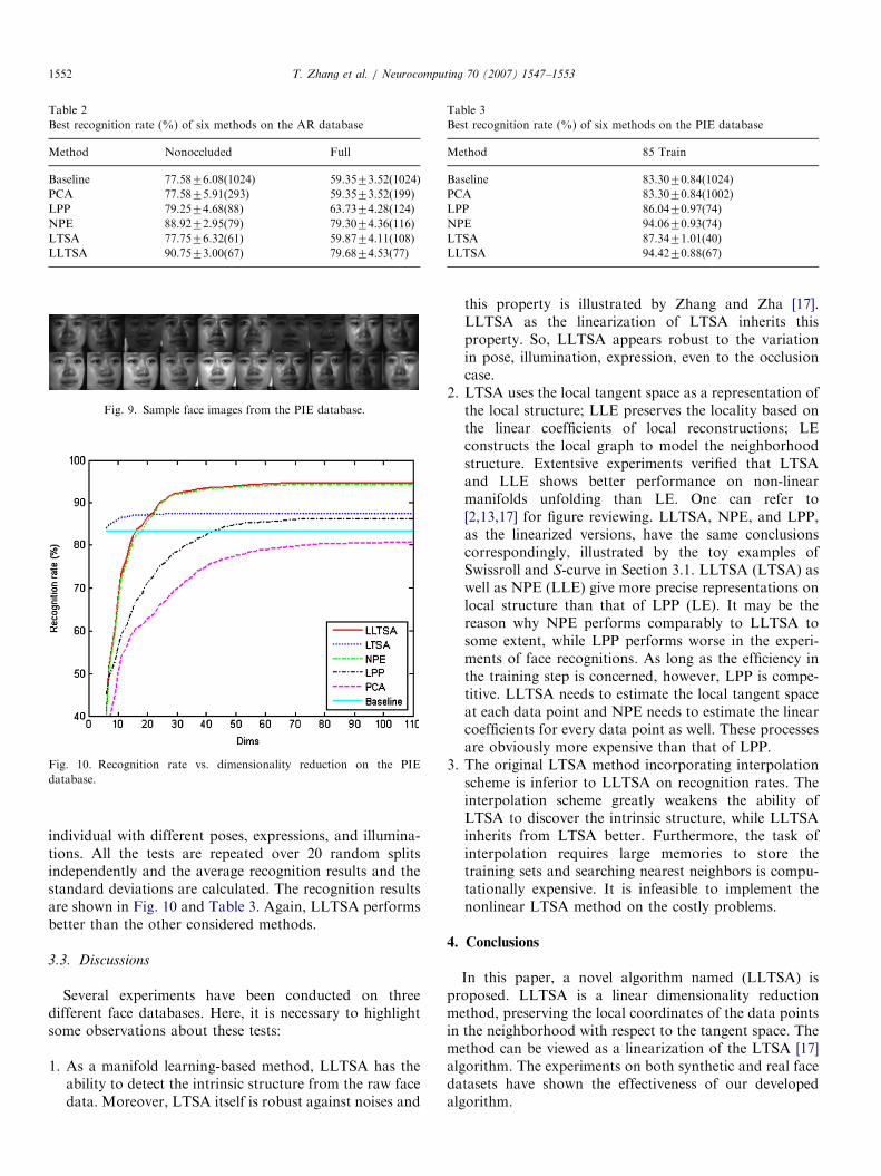
3.2.3. PIE

The PIE database [15] includes over 40,000 facial imagesof 68 people. We adopt the experimental strategy described

in [6]. One hundred and seventy near frontal face imagesfor each person are employed, 85 for training and the other85 for testing. Fig. 9 shows several sample images of an

ARTICLE IN PRESS

Table 2

Best recognition rate (%) of six methods on the AR database

Method Nonoccluded Full

Baseline 77.5876.08(1024) 59.3573.52(1024)

PCA 77.5875.91(293) 59.3573.52(199)

LPP 79.2574.68(88) 63.7374.28(124)

NPE 88.9272.95(79) 79.3074.36(116)

LTSA 77.7576.32(61) 59.8774.11(108)

LLTSA 90.7573.00(67) 79.6874.53(77)

Fig. 9. Sample face images from the PIE database.

Fig. 10. Recognition rate vs. dimensionality reduction on the PIE

database.

Table 3

Best recognition rate (%) of six methods on the PIE database

Method 85 Train

Baseline 83.3070.84(1024)

PCA 83.3070.84(1002)

LPP 86.0470.97(74)

NPE 94.0670.93(74)

LTSA 87.3471.01(40)

LLTSA 94.4270.88(67)

T. Zhang et al. / Neurocomputing 70 (2007) 1547–15531552

individual with different poses, expressions, and illumina-tions. All the tests are repeated over 20 random splitsindependently and the average recognition results and thestandard deviations are calculated. The recognition resultsare shown in Fig. 10 and Table 3. Again, LLTSA performsbetter than the other considered methods.

3.3. Discussions

Several experiments have been conducted on threedifferent face databases. Here, it is necessary to highlightsome observations about these tests:

1.

As a manifold learning-based method, LLTSA has theability to detect the intrinsic structure from the raw facedata. Moreover, LTSA itself is robust against noises and

this property is illustrated by Zhang and Zha [17].LLTSA as the linearization of LTSA inherits thisproperty. So, LLTSA appears robust to the variationin pose, illumination, expression, even to the occlusioncase.

2.

LTSA uses the local tangent space as a representation ofthe local structure; LLE preserves the locality based onthe linear coefficients of local reconstructions; LEconstructs the local graph to model the neighborhoodstructure. Extentsive experiments verified that LTSAand LLE shows better performance on non-linearmanifolds unfolding than LE. One can refer to[2,13,17] for figure reviewing. LLTSA, NPE, and LPP,as the linearized versions, have the same conclusionscorrespondingly, illustrated by the toy examples ofSwissroll and S-curve in Section 3.1. LLTSA (LTSA) aswell as NPE (LLE) give more precise representations onlocal structure than that of LPP (LE). It may be thereason why NPE performs comparably to LLTSA tosome extent, while LPP performs worse in the experi-ments of face recognitions. As long as the efficiency inthe training step is concerned, however, LPP is compe-titive. LLTSA needs to estimate the local tangent spaceat each data point and NPE needs to estimate the linearcoefficients for every data point as well. These processesare obviously more expensive than that of LPP.

3.

The original LTSA method incorporating interpolationscheme is inferior to LLTSA on recognition rates. Theinterpolation scheme greatly weakens the ability ofLTSA to discover the intrinsic structure, while LLTSAinherits from LTSA better. Furthermore, the task ofinterpolation requires large memories to store thetraining sets and searching nearest neighbors is compu-tationally expensive. It is infeasible to implement thenonlinear LTSA method on the costly problems.

4. Conclusions

In this paper, a novel algorithm named (LLTSA) isproposed. LLTSA is a linear dimensionality reductionmethod, preserving the local coordinates of the data pointsin the neighborhood with respect to the tangent space. Themethod can be viewed as a linearization of the LTSA [17]algorithm. The experiments on both synthetic and real facedatasets have shown the effectiveness of our developedalgorithm.

ARTICLE IN PRESST. Zhang et al. / Neurocomputing 70 (2007) 1547–1553 1553

Acknowledgments

The authors would like to thank the anonymousreviewers and editors for their comments and suggestions,which helped to improve the quality of this paper greatly.

References

[1] P.N. Belhumeur, J.P. Hespanha, D.J. Kriegman, Eigenfaces vs.

Fisherfaces: recognition using class specific linear projection, IEEE

Trans. Pattern Anal. Mach. Intell. 19 (7) (1997) 711–720.

[2] M. Belkin, P. Niyogi, Laplacian eigenmaps and spectral techniques

for embedding and clustering, in: Proceedings of Advances in Neural

Information Processing System, vol. 14, Vancouver, Canada,

December 2001.

[3] P. Comon, Independent component analysis. A new concept?, Signal

Process. 36 (3) (1994) 287–314.

[4] T. Cox, M. Cox, Multidimensional Scaling, Chapman & Hall,

London, 1994.

[5] X. He, P. Niyogi, Locality Preserving Projections, in: Proceedings of

Advances in Neural Information Processing System, vol. 16,

Vancouver, Canada, December 2003.

[6] X. He, S. Yan, Y. Hu, H. Zhang, Learning a locality preserving

subspace for visual recognition, in: Proceedings of Ninth Interna-

tional Conference on Computer Vision, France, October 2003,

pp. 385–392.

[7] X. He, D. Cai, S. Yan, H. Zhang, Neighborhood preserving

embedding, in: Proceedings of the 10 IEEE International Conference

on Computer Vision, Beijing, China, October 2005, pp. 1208–1213.

[8] http://ews.uiuc.edu/�dengcai2/Data/data.html.

[9] I.T. Jolliffe, Principal Component Analysis, Springer, New York,

1986.

[10] H. Li, L. Teng, W. Chen, I. Shen, Supervised learning on local

tangent space, in: Proceedings of the Second International Sympo-

sium on Neural Networks, Chongqing, China, May, 2005.

[11] A.M. Martinez, R. Benavente, The AR face database, CVC Technical

Report No. 24, June 1998.

[12] F. Samaria, A. Harter, Parameterisation of a stochastic model for

human face identification, in: Proceedings of the Second IEEE

Workshop on Applications of Computer Vision, Sarasota, USA,

December 1994.

[13] L. Saul, S. Roweis, Think globally, fit locally: unsupervised learning

of nonlinear manifolds, J. Mach. Learning Res. 4 (2003) 119–155.

[14] G. Shakhnarovich, B. Moghaddam, Face recognition in subspaces,

in: S.Z. Li, A.K. Jain (Eds.), Handbook of Face Recognition,

Springer, New York, 2004.

[15] T. Sim, S. Baker, M. Bsat, The CMU Pose, illumination, and

expression (PIE) database, in: Proceedings of the IEEE Inter-

national Conference on Automatic Face and Gesture Recognition,

Washington, DC, USA, May 2002.

[16] J. Tenenbaum, V. de Silva, J. Langford, A global geometric

framework for nonlinear dimensionality reduction, Science 290

(2000) 2319–2323.

[17] Z. Zhang, H. Zha, Principal manifolds and nonlinear dimensionality

reduction via tangent space alignment, SIAM J. Sci. Comput. 26 (1)

(2004) 313–338.

Tianhao Zhang was born in Shandong, China, in

November 1980. He received the Bachelor’s

degree in Electrical Engineering from Shandong

University in 2002, and the Master’s degree in

Power Machinery and Engineering from Chan-

gan University in 2005. Currently, he is a Ph.D.

candidate in Institute of Image Processing and

Pattern Recognition, Shanghai Jiao Tong Uni-

versity. His research interests include manifold

learning, face recognition and computer vision.

Jie Yang was born in Shanghai, China, in August

1964. He received a Ph.D. in computer in

Department of Computer, University of Ham-

burg, Germany. Dr. Yang is now the Professor

and Vice-director of Institute of Image Processing

and Pattern Recognition, Shanghai Jiao Tong

University. He is charged with more than 20

nation and ministry scientific research projects in

image processing, pattern recognition, data amal-

gamation, data mining, and artificial intelligence.

Deli Zhao was born in Anhui, China, in May

1980. He received his bachelor’s degree in

Electrical Engineering and Automation from

China University of Mining and Technology in

2003 and the master’s degree from Institute of

Image Processing and Pattern Recognition in

Shanghai Jiao Tong University in 2006. His

current research interests include linear and

nonlinear dimensionality reduction and feature

extraction.

Xinliang Ge was born in Hebei, China, in 1975.

Now he is a doctorial candidate in Institute of

Image Processing and Pattern Recognition,

Shanghai Jiao Tong University. His research

interests include 3D face recognition; facial

feature extraction; image processing.