let’s talk a little about getting around inside of excel · let’s talk a little about getting...

Let’s talk a little about getting around inside of Excel. For convenience sake, I’ll use the much abused term “navigate” to describe everything from moving around on a worksheet, w

Prepared by 2kmaro of DSLReports.com of 22 [email protected] Basic Excel Operations

ithin a workbook, and even cruising

most things in Windows, there re more than a couple of ways to do something. Starting Excel is no exception.

around on the hard drive looking for files.

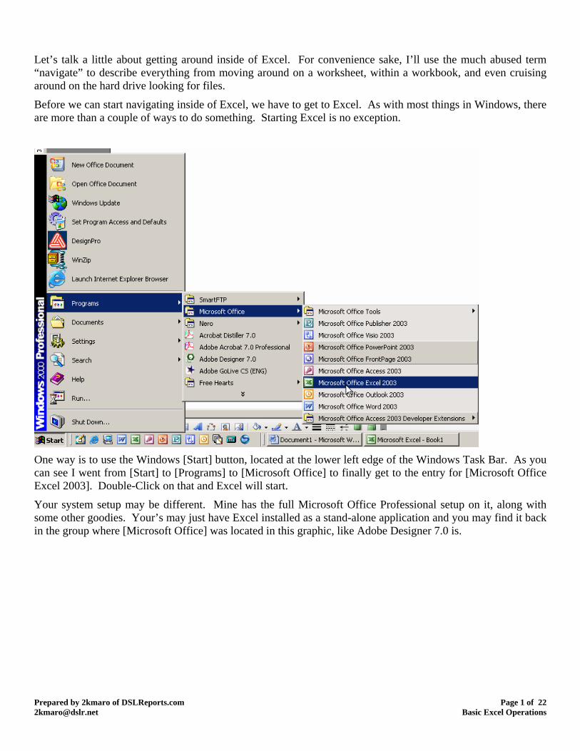
Before we can start navigating inside of Excel, we have to get to Excel. As with a

One way is to use the Windows [Start] button, located at the lower left edge of the Windows Task Bar. As you can see I went from [Start] to [Programs] to [Microsoft Office] to finally get to the entry for [Microsoft Office

may find it back in the group where [Microsoft Office] was located in this graphic, like Adobe Designer 7.0 is.

Excel 2003]. Double-Click on that and Excel will start.

Your system setup may be different. Mine has the full Microsoft Office Professional setup on it, along with some other goodies. Your’s may just have Excel installed as a stand-alone application and you

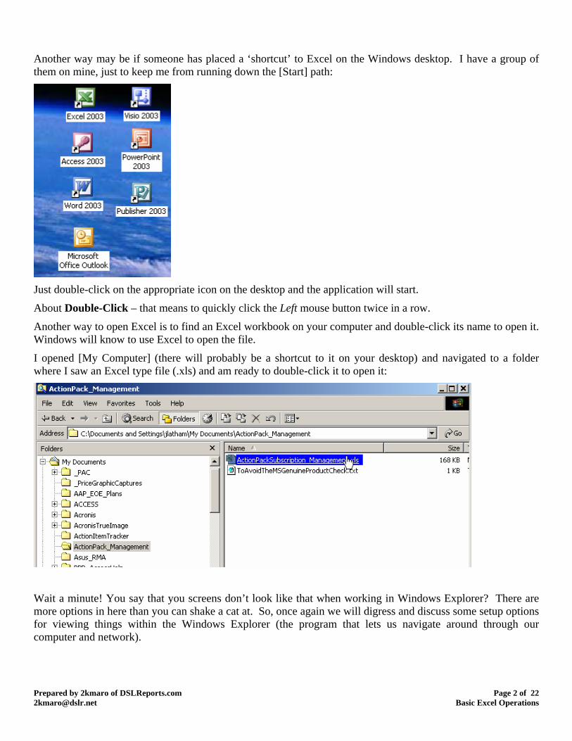
Another way may be if someone has placed a ‘shortcut’ to Excel o


n the Windows desktop. I have a group of from running down the [Start] path: them on mine, just to keep me

Just double-click on the appropriate icon on the desktop and the application will start.

About Double-Click – that means to quickly click the Left mouse button twice in a row.

Another way to open Excel is to find an Excel workbook on your computer and double-click its name to open it.

ktop) and navigated to a folder

Windows will know to use Excel to open the file.

I opened [My Computer] (there will probably be a shortcut to it on your deswhere I saw an Excel type file (.xls) and am ready to double-click it to open it:

in the Windows Explorer (the program that lets us navigate around through our computer and network).

Wait a minute! You say that you screens don’t look like that when working in Windows Explorer? There are more options in here than you can shake a cat at. So, once again we will digress and discuss some setup options for viewing things with

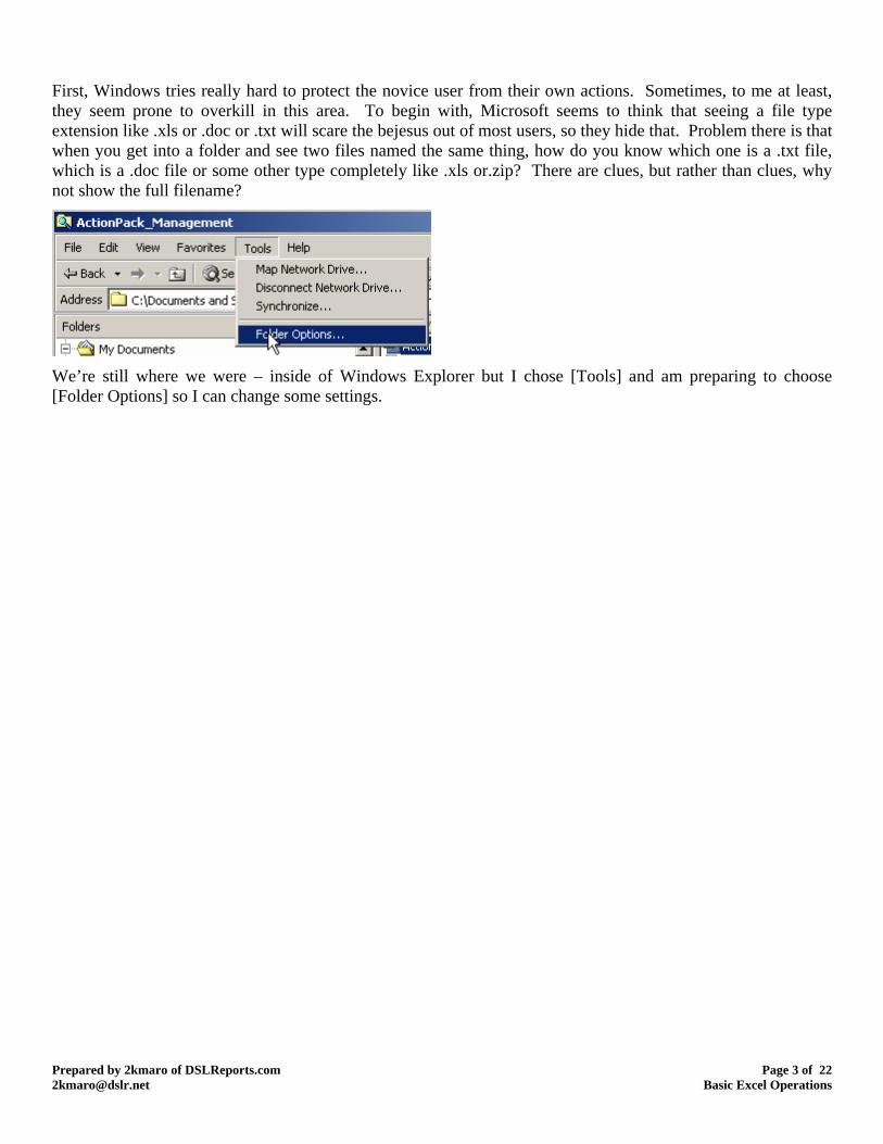
First, Windows tries really hard to protect the novice user from their own actions. Sometimes, to me at least, they seem prone to overkill in this area. To begin with, Microsoft seems to think that seeing a file type extension like .xls or .doc or .txt will scare the bejesus out of most users, so they hide that. Problem there is that when you get into a folder and see two files named the same thing, how do you know which one is a .txt file, which is a .doc file or some


other type completely like .xls or.zip? There are clues, but rather than clues, why not show the full filename?

We’re still where we were – inside of Windows Explorer but I chose [Tools] and am preparing to choose [Folder Options] so I can change some settings.

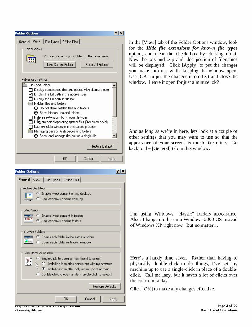
In the [View] tab of the Folder Options window, look for the Hide file extensions for known file types option, and clear the check box by clicking on it. Now the .xls and .zip and .doc portion of filenames will be displayed. Click [Apply] to put the changes you make into use while keeping the window open. Use [OK] to put the changes into effect and close the

indow. Leave it open for just a minute, ok?

mine. Go ack to the [General] tab in this window.

instead f Windows XP right now. But no matter…

but it saves a lot of clicks over

w

And as long as we’re in here, lets look at a couple of other settings that you may want to use so that the appearance of your screens is much likeb


I’m using Windows “classic” folders appearance. Also, I happen to be on a Windows 2000 OSo

Here’s a handy time saver. Rather than having to physically double-click to do things, I’ve set my machine up to use a single-click in place of a double-click. Call me lazy,the course of a day.

Click [OK] to make any changes effective.

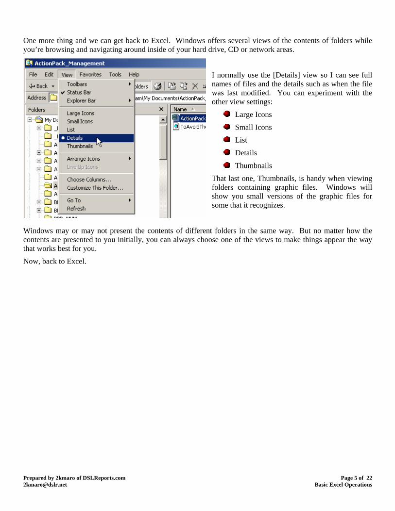
One more thing and we can get back to Excel. Windows offersyou’re browsing and navigating around inside of your hard

several views of the contents of folders while d

e details such as when the file was You can experiment with the oth

rive, CD or network areas.

I normally use the [Details] view so I can see full names of files and th

last modified. er view settings:


Icons Large

Small Icons List Details

Thumbnails

That last one, Thumbnails, is handy when viewing folders containing graphic files. Windows will how you small versions of the graphic files for

e that it recognizes.

ot present the contents of different folders in the same way. But no matter how the to you initially, you can always choose one of the views to make things appear the way

Now, back to Excel.

ssom

Windows may or may ncontents are presentedthat works best for you.

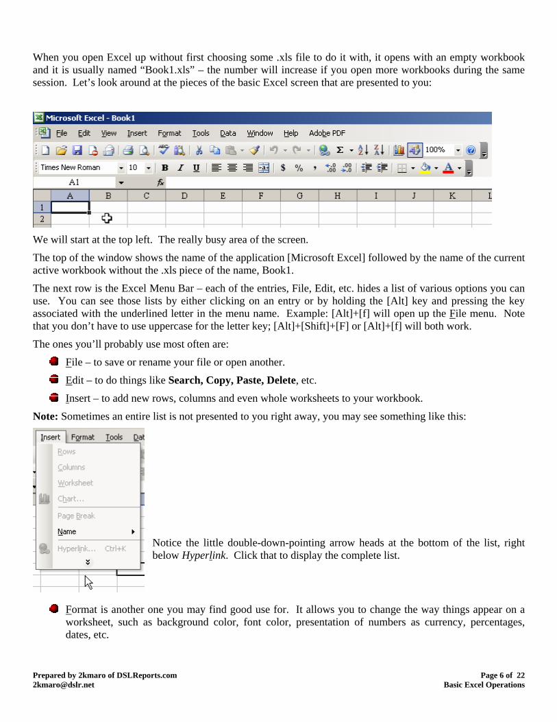
When you open Excel up without first choosing some .xls file to do it with, it opens with an empty workbook and it is usually named “Book1.xls” – the number will increase if you open more workbooks during the same

ssion. Let’s look around at the pieces of the basic Excel screen that are presented to you: se

icrosoft Excel] followed by the name of the current

We will start at the top left. The really busy area of the screen.

The top of the window shows the name of the application [Mactive workbook without the .xls piece of the name, Book1.

The next row is the Excel Menu Bar – each of the entries, File, Edit, etc. hides a list of various options you can use. You can see those lists by either clicking on an entry or by holding the [Alt] key and pressing the key associated with the underlined letter in the menu name. Example: [Alt]+[f] will open up the File menu. Note

tter key; [Alt]+[Shift]+[F] or [Alt]+[f] will both work.

The

that you don’t have to use uppercase for the le

ones you’ll probably use most often are:

File – to save or rename your file or open another. Edit – to do things like Search, Copy, Paste, Delete, etc.

Insert – to add new rows, columns and even whole worksheets to your workbook.


Note: Sometimes an entire list is not presented to you right away, you may see something like this:

e bottom of the list, right elow Hyperl

Notice the little double-down-pointing arrow heads at thb ink. Click that to display the complete list.

Format is another one you may find good use for. It allows you to change the way things appear on a worksheet,

such as background color, font color, presentation of numbers as currency, percentages,

dates, etc.


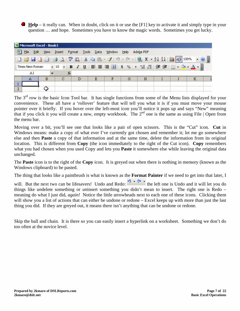
Help – it really can. When in doubt, click on it or use the [F1] key to activate it and simply type in your question … and hope. Sometimes you have to know the magic words. Sometimes you get lucky.

The 3rd row is the basic Icon Tool bar. It has single functions from some of the Menu lists displayed for your convenience. These all have a ‘rollover’ feature that will tell you what it is if you must move your mouse pointer over it briefly. If you hover over the left-most icon you’ll notice it pops up and says “New” meaning that if you click it you will create a new, empty workbook. The 2nd one is the same as using File | Open from

chosen when you used Copy and lets you Paste it somewhere else while leaving the original data

Copy icon. It is greyed out when there is nothing in memory (known as the

the menu bar.

Moving over a bit, you’ll see one that looks like a pair of open scissors. This is the “Cut” icon. Cut in Windows means: make a copy of what ever I’ve currently got chosen and remember it; let me go somewhere else and then Paste a copy of that information and at the same time, delete the information from its original location. This is different from Copy (the icon immediately to the right of the Cut icon). Copy remembers what you hadunchanged.

The Paste icon is to the right of the Windows clipboard) to be pasted.

The thing that looks like a paintbrush is what is known as th t Painter if we need to get into that later, I

will. But the next two can be lifesavers! Undo and Redo:

e Forma

the left one is Undo and it will let you do things like undelete something or uninsert something you didn’t mean to insert. The right one is Redo – meaning do what I just did, again! Notice the little arrowheads next to each one of these icons. Clicking them will show you a list of actions that can either be undone or redone – Excel keeps up with more than just the last

ing you did. If they are greyed out, it means there isn’t anything that can be undone or redone.

there so you can easily insert a hyperlink on a worksheet. Something we don’t do o often at the novice level.

th

Skip the ball and chain. It is to


Autosum – one of my personal favorites. We will talk in more detail about it later. But essentially it provides a shortcut way to work with a large number of cells to obtain their Sum, Average,

aximum value in the list, minimum value in the list, etc. It’s fairly smart also.

m

Sorting: Be very careful using these. Excel is weird at times when it comes to sorting, and can really mess up your day if you don’t know how it handles sorts. I’ll definitely get into that later on for your own

The next two icons have to do with charting and using drawing objects (squares, shapes, etc).

protection.

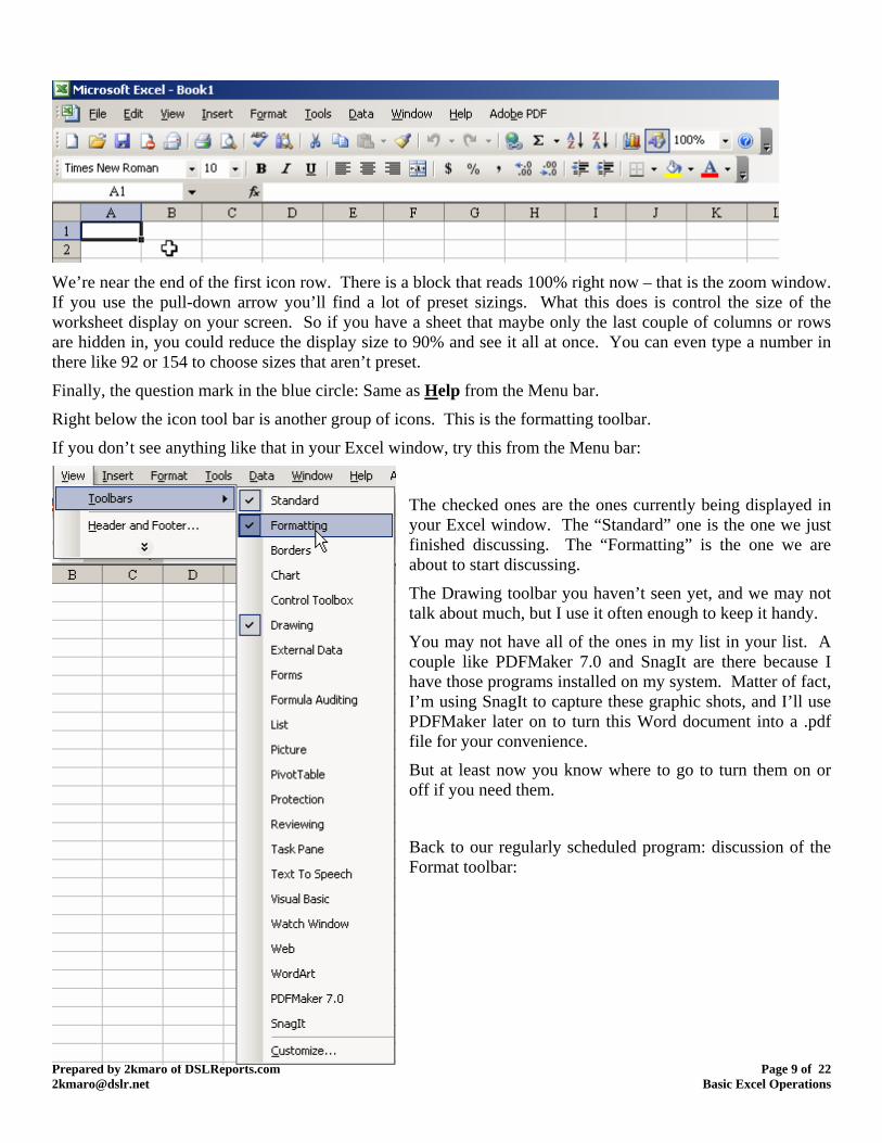
We’re near the end of the first icon row. There is a block that reads 100% right now – that is the zoom window. If you use the pull-down arrow you’ll find a lot of preset sizings. What this does is control the size of the worksheet display on your screen. So if you have a sheet that maybe only the last couple of columns or rows are hidden in, you could reduce the display size to 90% and see it all at once. You can even type a number in there like 92 or 154 to choose sizes that aren’t preset.

Finally, the question mark in the blue circle: Same as Help from the Menu bar.

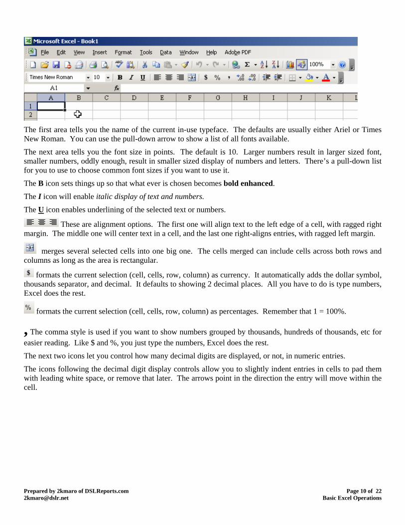
Right below the icon tool bar is another group of icons. This is the formatting toolbar.


If you don’t see anything like that in your Excel window, try this from the Menu bar:

matting” is the one we are

t

this Word document into a .pdf

know where to go to turn them on or ff if you need them.

larly scheduled program: discussion of the Format toolbar:

The checked ones are the ones currently being displayed in your Excel window. The “Standard” one is the one we just finished discussing. The “Forabout to start discussing.

The Drawing toolbar you haven’t seen yet, and we may notalk about much, but I use it often enough to keep it handy.

You may not have all of the ones in my list in your list. A couple like PDFMaker 7.0 and SnagIt are there because I have those programs installed on my system. Matter of fact, I’m using SnagIt to capture these graphic shots, and I’ll use PDFMaker later on to turnfile for your convenience.

But at least now you o

Back to our regu


The first area tells you the name of the current in-use typeface. The defaults are usually either Ariel or Times

numbers and letters. There’s a pull-down list

mes bold enhanced.

New Roman. You can use the pull-down arrow to show a list of all fonts available.

The next area tells you the font size in points. The default is 10. Larger numbers result in larger sized font, smaller numbers, oddly enough, result in smaller sized display offor you to use to choose common font sizes if you want to use it.

The B icon sets things up so that what ever is chosen beco

The I icon will enable italic display of text and numbers.

The U icon enables underlining of the selected text or numbers.

These are alignment options. The first one will align text to the left edge of a cell, with ragged right margin. The middle one will center text in a cell, and the last one right-aligns entries, with ragged left margin.

merges several selected cells into one big one. The cells merged can include cells across both rows and columns as long as the area is rectangular.

formats the current selection (cell, cells, row, column) as currency. It automatically adds the dollar symbol, thousands separator, and decimal. It defaults to showing 2 decimal places. All you have to do is type numbers, Excel does the rest.

formats the current selection (cell, cells, row, column) as percentages. Remember that 1 = 100%.

ds, hundreds of thousands, etc for

eading white space, or remove that later. The arrows point in the direction the entry will move within the cell.

, The comma style is used if you want to show numbers grouped by thousaneasier reading. Like $ and %, you just type the numbers, Excel does the rest.

The next two icons let you control how many decimal digits are displayed, or not, in numeric entries.

The icons following the decimal digit display controls allow you to slightly indent entries in cells to pad them with l


ions of borders by using F

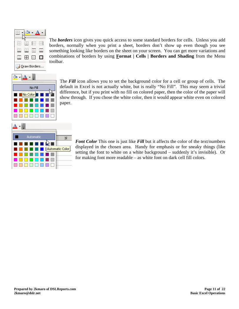
The borders icon gives you quick access to some standard borders for cells. Unless you add borders, normally when you print a sheet, borders don’t show up even though you see something looking like borders on the sheet on your screen. You can get more variations and combinat ormat | Cells | Borders and Shading from the Menu toolbar.

rough. If you chose the white color, then it would appear white even on colored aper.

ible). Or r making font more readable – as white font on dark cell fill colors.

The Fill icon allows you to set the background color for a cell or group of cells. The default in Excel is not actually white, but is really “No Fill”. This may seem a trivial difference, but if you print with no fill on colored paper, then the color of the paper will show thp

Font Color This one is just like Fill but it affects the color of the text/numbers displayed in the chosen area. Handy for emphasis or for sneaky things (like setting the font to white on a white background – suddenly it’s invisfo

Finally! We get to the meat of the matter. Actually doing work with a workbook and worksheets in it.

Lets start with security. When opening some workbooks you may get one of a couple of warnings or alerts about “Macros”. A macro in Excel is actually full-blown programming code. With code and the righ


t

ng the needed code while still protecting you from workbooks where you might not be expecting code to exist:

tart by going to the Security settings for Macro code.

permissions, anything can be done including renaming or even destroying files on your system or the network.

Some of the workbooks we’ve prepared with this data include such code. Excel comes “out of the box” set up to prevent running such code at all. That won’t quite do for us. Here’s how to adjust the Macro Security level to permit runni

S

Choose the Medium setting, not the Low setting. Even I don’t set my system to Low and 98% of all macro code in my Excel books I wrote myself. I

st don’t like unexpected surprises.

el and re-open it to get the setting to be recognized.

ju

With this setting you’ll always be prompted to either Enable or Disable macros in a workbook. For the ones used on this project, we will need touse Enabled to get the automated features to work.

After changing this setting you need to close Exc

Where to start? So much to possibly cover. Books of several hundred pages have been written about using Excel, how to get around in it, and how to make it really work for you. I am going to go on the premise that you’re not necessarily creating new workbooks, but instead are working with som


e that have already been nalysis. created and you just need to get around in them and perhaps do a little data a

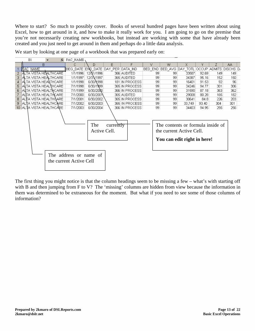
We start by looking at one page of a workbook that was prepared early on:

rmined to be extraneous for the moment. But what if you need to see some of those columns of information?

The first thing you might notice is that the column headings seem to be missing a few – what’s with starting off with B and then jumping from F to V? The ‘missing’ columns are hidden from view because the information in them was dete

The address or name of the current Active Cell

The currently Active Cell.

The contents or formula inside of the current Active Cell.

You can edit right in here!

Easiest way to view them would be to click on any row number on the left side of the sheet – this would highlight that entire row. Then use the Menu tool bar to unhide all column . This picture shows that process: s

First I clicked on the “3” to select all of row 3. As I said, any row number would work. Then I went to Format | Column | Unhide


to get all of the olumns displayed.

ell de-select (unselect?) the row.

letter/number to select the entire column/row and then use F

c

As you can see, all columns have become visible. Row 3 still remains selected. Click on any cto

Ok, that was nice, but now I want to hide a column (or row) to get it out of view. To hide one column or row at a time, just click it’s ormat | Column | Hide to

mething else. At this point you can elect to perform some operations that will affect

remove it from view.

Need to hide more than one at a time? I’ll give examples for columns, but the procedures apply to rows also.

Dragging – you have to understand dragging first. To ‘drag’ in Windows means to click at an inclusive starting point and without releasing the left mouse button drag the mouse over a series of objects to be included in an action. At the end of the group you release the mouse button and all the things you dragged over will remain selected until you select sothe entire selected group.

Hiding contiguous columns (or rows) Click the first column identifier that you want to end up hidden. Drag the mouse across the other column identifiers until you’ve chosen all to be hidden that are side by side. Then use Format | Column | Hide to hide them. You can do the reverse to unhide some at times. Assume that columns B, C and D are hidden. You could drag from A to E (which would include B, C and D) and then Format | Column | Unhide to display those columns.

Hiding columns that are not contiguous. Click the first column to be hidden, then to choose additional columns to be hidden press the [Ctrl] key and hold it while clicking on other columns. You can release the [Ctrl] key in between selecting columns. When you do this kind of operation, I recommend that you stop and Format | Column | Hide to take care of them in groups, because if you mess up and select one you didn’t mean to, it’s

ted columns. difficult to back out of the process without losing selection of all the previously selec

These s


ame selection methods (click, click-and-drag and [Ctrl]+click) will work on:

acilitate hiding columns in our workbook. Take a look at the

g in a bit. Lets continue looking at dealing with Rows, Columns and Cells on

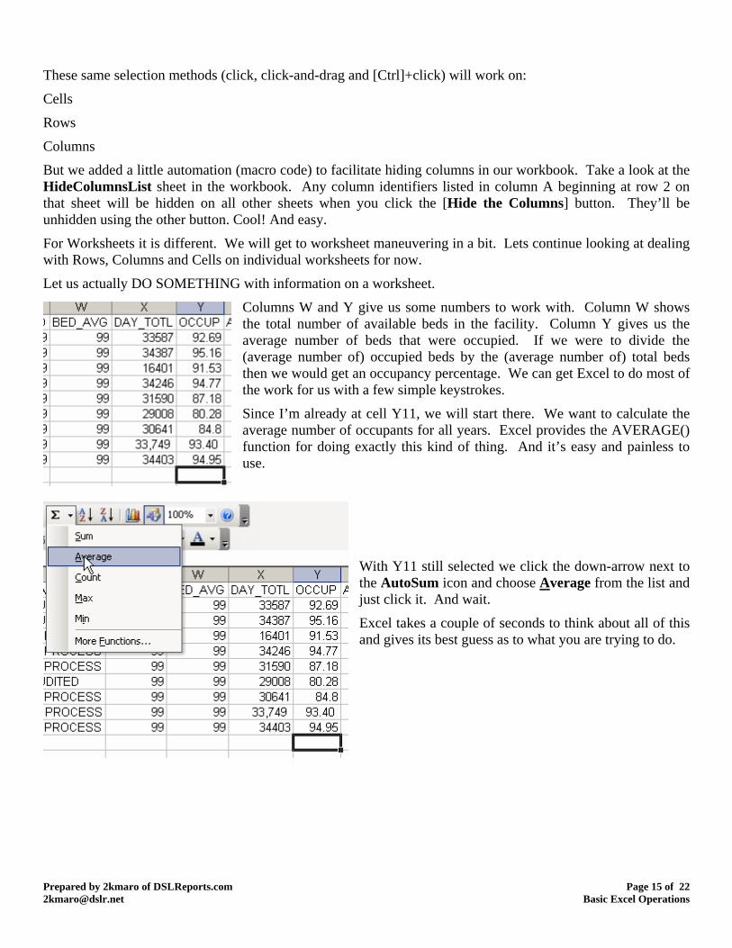
Let us actually DO SOMETHING

. If we were to divide the

I’m already at cell Y11, we will start there. We want to calculate the verage number of occupants for all years. Excel provides the AVERAGE() nction for doing exactly this kind of thing. And it’s easy and painless to

use.

Cells

Rows

Columns

But we added a little automation (macro code) to fHideColumnsList sheet in the workbook. Any column identifiers listed in column A beginning at row 2 on that sheet will be hidden on all other sheets when you click the [Hide the Columns] button. They’ll be unhidden using the other button. Cool! And easy.

For Worksheets it is different. We will get to worksheet maneuverin individual worksheets for now.

with information on a worksheet.

Columns W and Y give us some numbers to work with. Column W shows the total number of available beds in the facility. Column Y gives us the average number of beds that were occupied(average number of) occupied beds by the (average number of) total beds then we would get an occupancy percentage. We can get Excel to do most of the work for us with a few simple keystrokes.

Sinceafu

With Y11 still selected we click the down-arrow next to the AutoSum icon and choose Average from the list and just click it. And wait.

Excel takes a couple of seconds to think about all of this and gives its best guess as to what you are trying to do.


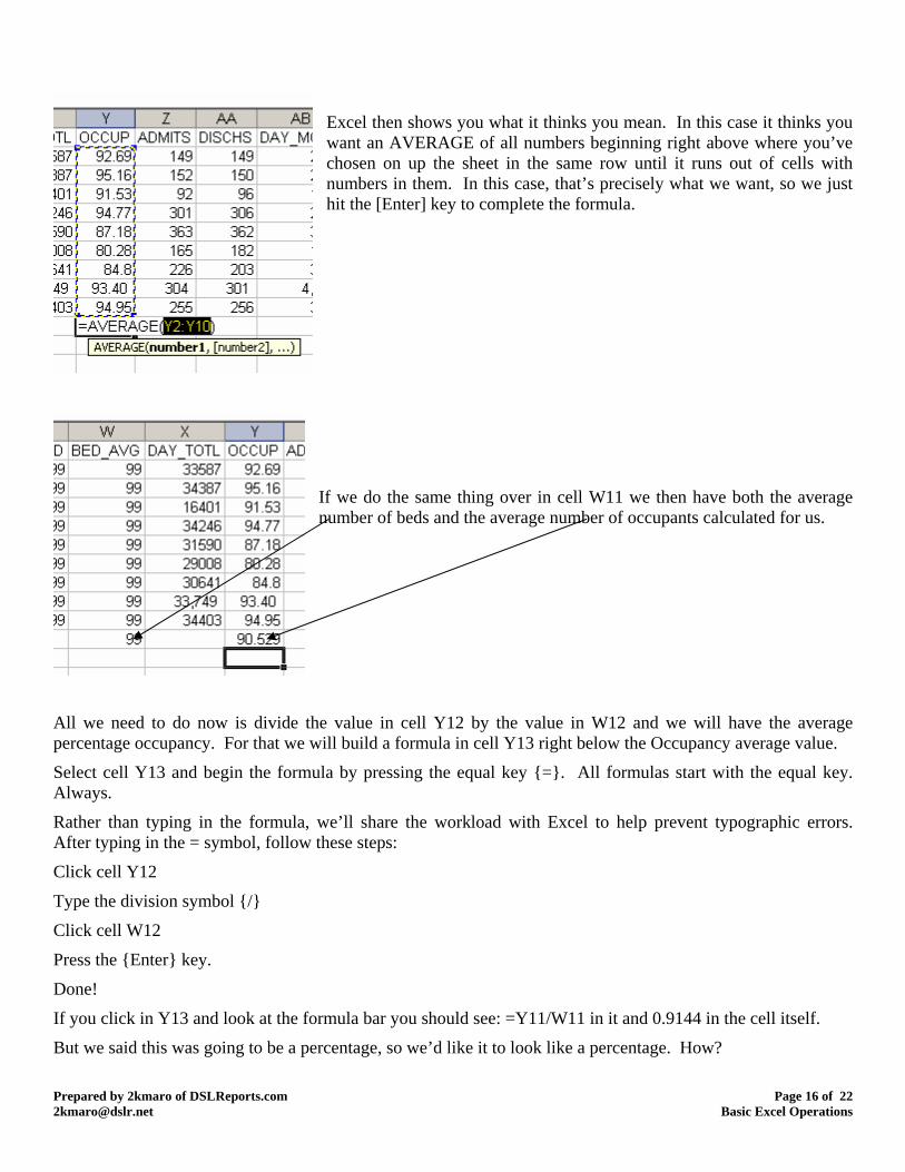
Excel then shows you what it thinks you mean. In this case it thinks you want an AVERAGE of all numbers beginning right above where you’ve chosen on up the sheet in the same row until it runs out of cells with numbers in them. In this case, that’s precisely what we want, so we just

it the [Enter] key to complete the formula.

ge umber of beds and the average number of occupants calculated for us.

e

ll Y13 and begin the formula by pressing the equal key {=}. All formulas start with the equal key.

the workload with Excel to help prevent typographic errors. the = symbol, follow these steps:

n symbol {/}

e {Enter} key.

he cell itself.

But we said this was going to be a percentage, so we’d like it to look like a percentage. How?

h

If we do the same thing over in cell W11 we then have both the averan

All we need to do now is divide the value in cell Y12 by the value in W12 and we will have the averagpercentage occupancy. For that we will build a formula in cell Y13 right below the Occupancy average value.

Select ceAlways.

Rather than typing in the formula, we’ll share After typing in

Click cell Y12

Type the divisio

Click cell W12

Press th

Done!

If you click in Y13 and look at the formula bar you should see: =Y11/W11 in it and 0.9144 in t

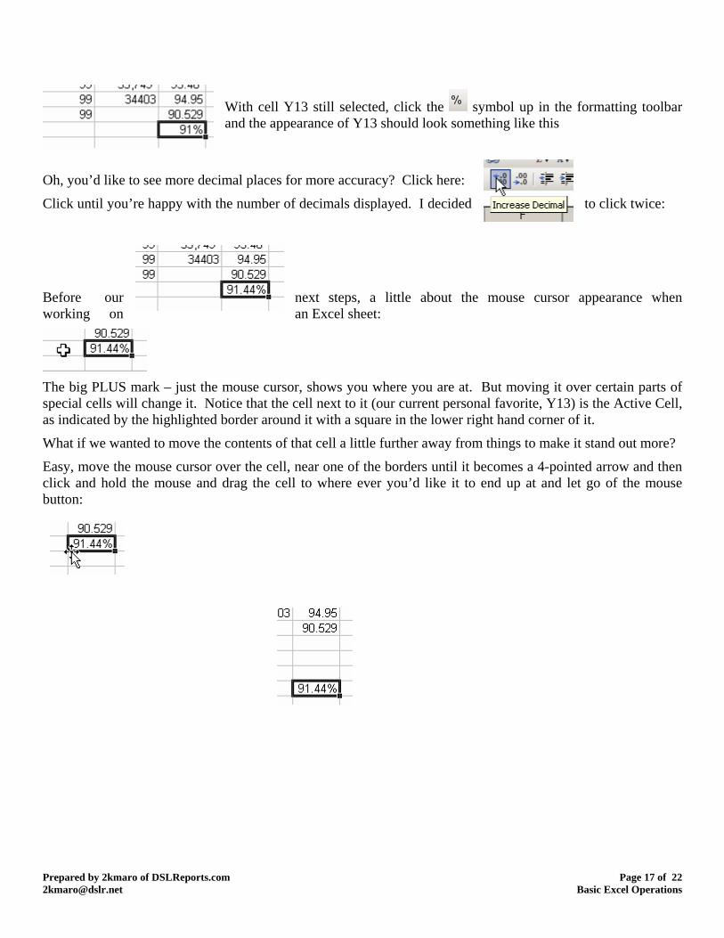
With cell Y13 still selected, click the symbol up in the


formatting toolbar and the appearance of Y13 should look something like this

lick until you’re happy with the number of ed. I decided to click twice:

our ittle about the mouse cursor appearance when an Excel sheet:

Oh, you’d like to see more decimal places for more accuracy? Click here:

C decimals display

Before next steps, a lworking on

The big PLUS mark – just the mouse cursor, shows you where you are at. But moving it over certain parts of special cells will change it. Notice that the cell next to it (our current personal favorite, Y13) is the Active Cell,

hold the mouse and drag the cell to where ever you’d like it to end up at and let go of the mouse button:

as indicated by the highlighted border around it with a square in the lower right hand corner of it.

What if we wanted to move the contents of that cell a little further away from things to make it stand out more?

Easy, move the mouse cursor over the cell, near one of the borders until it becomes a 4-pointed arrow and then click and

Our next adventure begins here. Earlier we set up the =AVERAGE() formulas for a couple of columns of information. What if we needed to set up the =AVERAGE() formula for many, many columns. Lots of tedious work to do it even with some of the

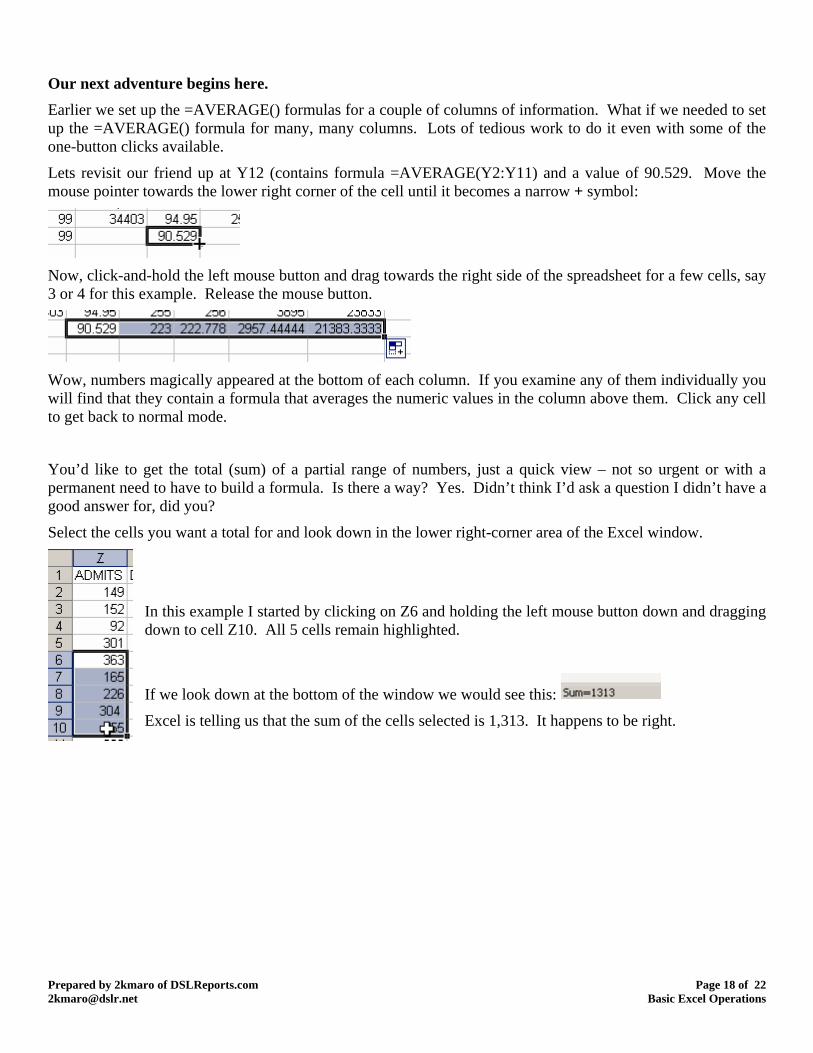
0.529. Move the er of the cell until it becomes a narrow + symbol:

one-button clicks available.

Lets revisit our friend up at Y12 (contains formula =AVERAGE(Y2:Y11) and a value of 9mouse pointer towards the lower right corn

Now, click-and-hold the left mouse button and drag towards the right side of the spreadsheet for a few cells, say 3 or 4 for this example. Release the mouse button.

Wow, numbers magically appeared at the bottom of each column. If you examine any of them individually you will find that they contain a f


ormula that averages the numeric values in the column above them. Click any cell get back to normal mode.

build a formula. Is there a way? Yes. Didn’t think I’d ask a question I didn’t have a

Select the cells you want a total for and look down in the lower right-corner area of the Excel window.

ing the left mouse button down and dragging own to cell Z10. All 5 cells remain highlighted.

to

You’d like to get the total (sum) of a partial range of numbers, just a quick view – not so urgent or with a permanent need to have to good answer for, did you?

In this example I started by clicking on Z6 and holdd

If we look down at the bottom of the window we would see this:

Excel is telling us that the sum of the cells selected is 1,313. It happens to be right.

What about working with values in cells from other sheets in the workbook? Using the point and click method to choose cells on other sheets, you can build formulas anywhere in the workbook that will properly reference the specific sheet and cell address. Saves lots of typing and reduces chance of error. You can actually build formulas referencing cells in other sheets in OTHER WORKBOOKS. But that creates some issues later of the availability of those workbooks because Excel wants to update the information from them to make sure it hasn’t changed, and if it cannot get to one of them it has no choice but to use the last known value from the other

? What to do? using the copy. The original will remain unchanged.

book and from the Menu bar choose

E

workbook(s).

I want to work with some of the information on a worksheet but I’m afraid I’ll mess it upMake a copy of the worksheet and work

How to make a copy of a worksheet:

Choose the sheet in your work


dit | Move or Copy Sheet

y] otherwise you will

I made another copy of the Alta Vista

is one to where the original had been and name it back to plain Alta Vista.

n Right-click (click on it using the right mouse button) on it’s tab and choose from the menu that come up:

Be sure and check the little box that says [Create a copjust move the sheet and still be working on the original.

The new sheet will be placed where you choose to put it in the middle area of the form (at the start of the workbook is the default) and will be given a number. For example, I’d previously copied the Alta Vista sheet to play with here and it became Alta Vista (2). If sheet, it would become Alta Vista (3).

Later, if your work went well on the Alta Vista (2) sheet, you could delete the original Alta Vista sheet, move thre

How to rename a sheet? Easiest way is to double-click on its name in the tab at the bottom of the sheet and work directly on it there. Or you ca

s

These are the options you can get when you right-click on a sheet’s name tab.

Use caution with the Delete option – once you delete a sheet there is no such thing as Undo. The Move or Copy option here brings up the dialog we just discussed and you pick up from there.

If you’re wondering about the Tab Color option, it’s fun. It sets the color for the tab of the currently selected sheet. This can give you a quick visual clue to

s location later on.

it

How do I correct a mistake made in a cell? Depends on the kind of mistake. If it is drastic and you just want to start all over, select the cell and hit the

elect the cell and edit the content where it’s shown in the formula bar. Hit [Enter] hen you are done editing.

[Del] key. Poof, all gone.

If it is correctable you can sw

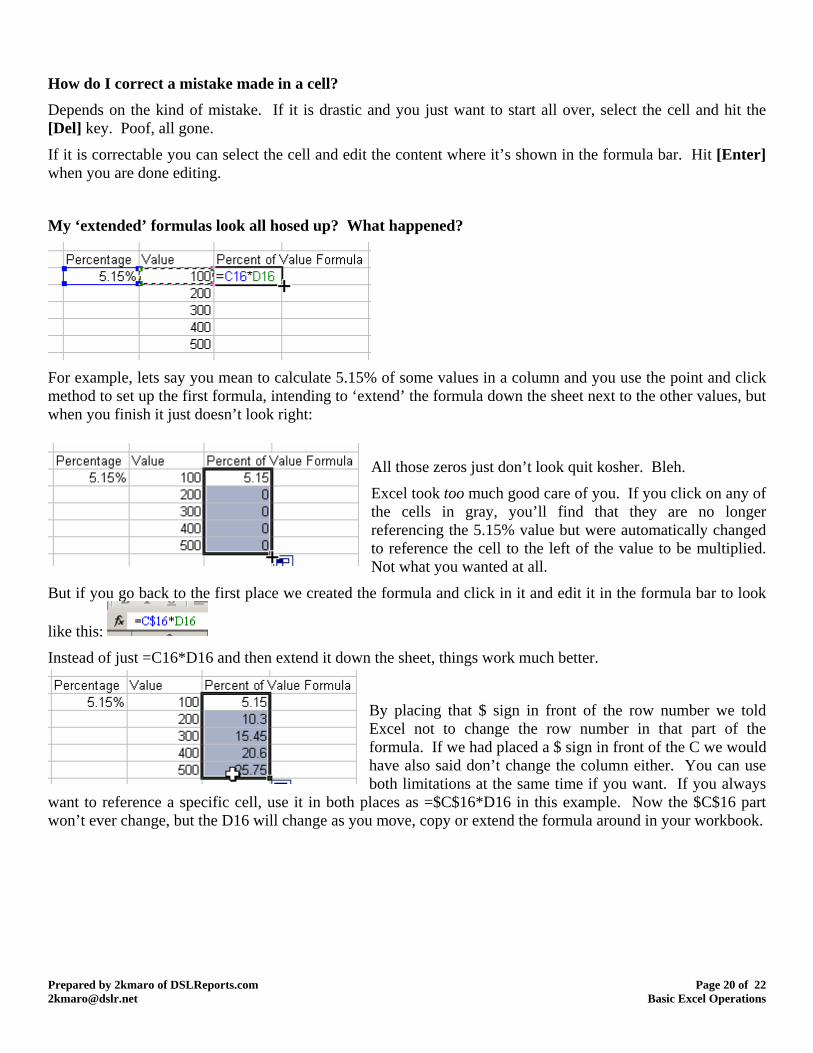
My ‘extended’ formulas look all hosed up? What happened?

For example, lets say you mean to calculate 5.15% of some values in a column and you use the point and click method to set up the first formula, intendin


g to ‘extend’ the formula down the sheet next to the other values, but when you finish it just doesn’t look right:

eft of the value to be multiplied.

mula and click in it and edit it in the formula bar to look

All those zeros just don’t look quit kosher. Bleh.

Excel took too much good care of you. If you click on any of the cells in gray, you’ll find that they are no longer referencing the 5.15% value but were automatically changed to reference the cell to the lNot what you wanted at all.

But if you go back to the first place we created the for

like this:

Instead of just =C16*D16 and then extend it down the sheet, things work much better.

won’t ever change, but the D16 will change as you move, copy or extend the formula around in your workbook.

By placing that $ sign in front of the row number we told Excel not to change the row number in that part of the formula. If we had placed a $ sign in front of the C we would have also said don’t change the column either. You can use both limitations at the same time if you want. If you always

want to reference a specific cell, use it in both places as =$C$16*D16 in this example. Now the $C$16 part

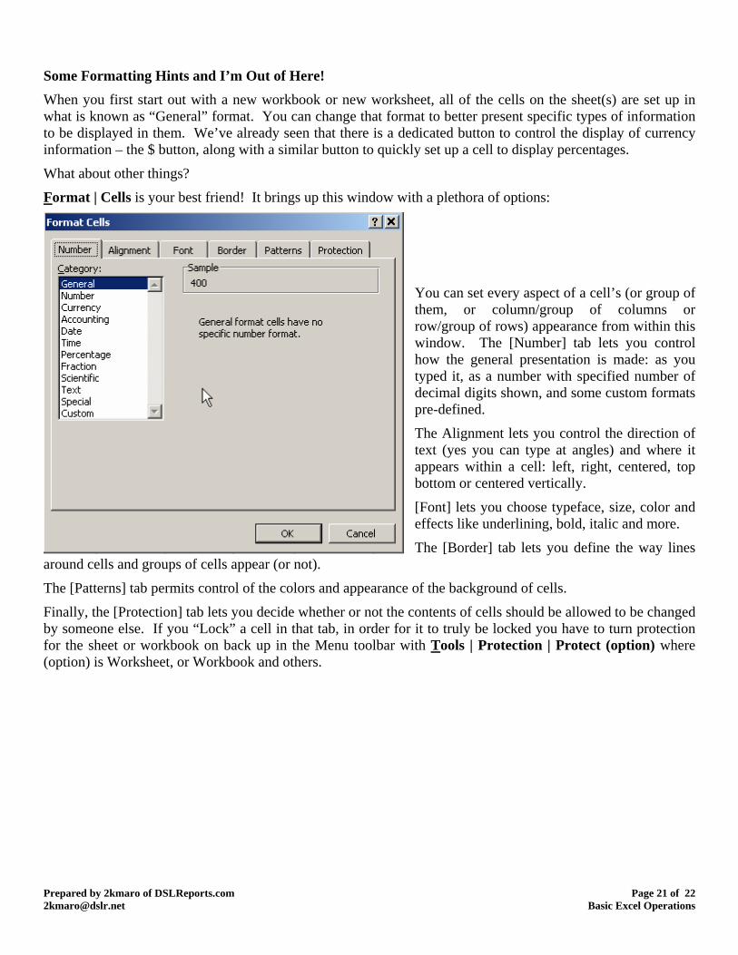
Some Formatting Hints and I’m Out of Here! When you first start out with a new workbook or new worksheet, all of the cells on the sheet(s) are set up in what is known as “General” format. You can change that format to better present specific types of information to be displayed in them. We’ve already seen that there is a dedicated button to control the display of currency

, along with a similar button to quickly set up a cell to display percentages.

F

information – the $ button

What about other things?


ormat | Cells is your best friend! It brings up this window with a plethora of options:

s shown, and some custom formats

ht, centered, top

d

The [Border] tab lets you define the way lines

enu toolbar with T

You can set every aspect of a cell’s (or group of them, or column/group of columns or row/group of rows) appearance from within this window. The [Number] tab lets you control how the general presentation is made: as you typed it, as a number with specified number of decimal digitpre-defined.

The Alignment lets you control the direction of text (yes you can type at angles) and where it appears within a cell: left, rigbottom or centered vertically.

[Font] lets you choose typeface, size, color aneffects like underlining, bold, italic and more.

around cells and groups of cells appear (or not).

The [Patterns] tab permits control of the colors and appearance of the background of cells.

Finally, the [Protection] tab lets you decide whether or not the contents of cells should be allowed to be changed by someone else. If you “Lock” a cell in that tab, in order for it to truly be locked you have to turn protection for the sheet or workbook on back up in the M ools | Protection | Protect (option) where

ption) is Worksheet, or Workbook and others.

(o

Sorting I promised you a little information about sorting to try and help keep you out of trouble.

hat is chosen! Put succinctly: Excel ONLY SORTS w

So lets say you have a set up like this

And we want to sort it alphabetically by name. We might think that we can just choose column A or the entries in Column A and choose the A-Z sort button and be done with it. Not necessarily true. In this case if you click

button, things DO work as expected and you get: in cell A1 and click that

Ages and eye color followed the names.

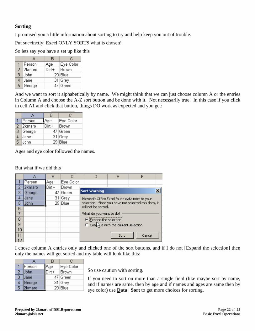
But what if we did this

I chose column A entries only and clicked one of the sort butt


ons, and if I do not [Expand the selection] then only the names will get sorted and my table will look like this:

are same then by eye color) use D

So use caution with sorting.

If you need to sort on more than a single field (like maybe sort by name, and if names are same, then by age and if names and ages

ata | Sort to get more choices for sorting.

let’s talk a little about getting around inside of excel · let’s talk a little about getting...

Documents