lesson 1: molecular electric conduction i. the density of
TRANSCRIPT
Note on: Methods of theoretical chemistry Prof. Roi Baer
Lesson 1: Molecular electric conduction
I. The density of states in a 1D quantum wire
Consider a quantum system with discrete en-
ergy levels 𝐸𝑛, 𝑛 = 1,2, …
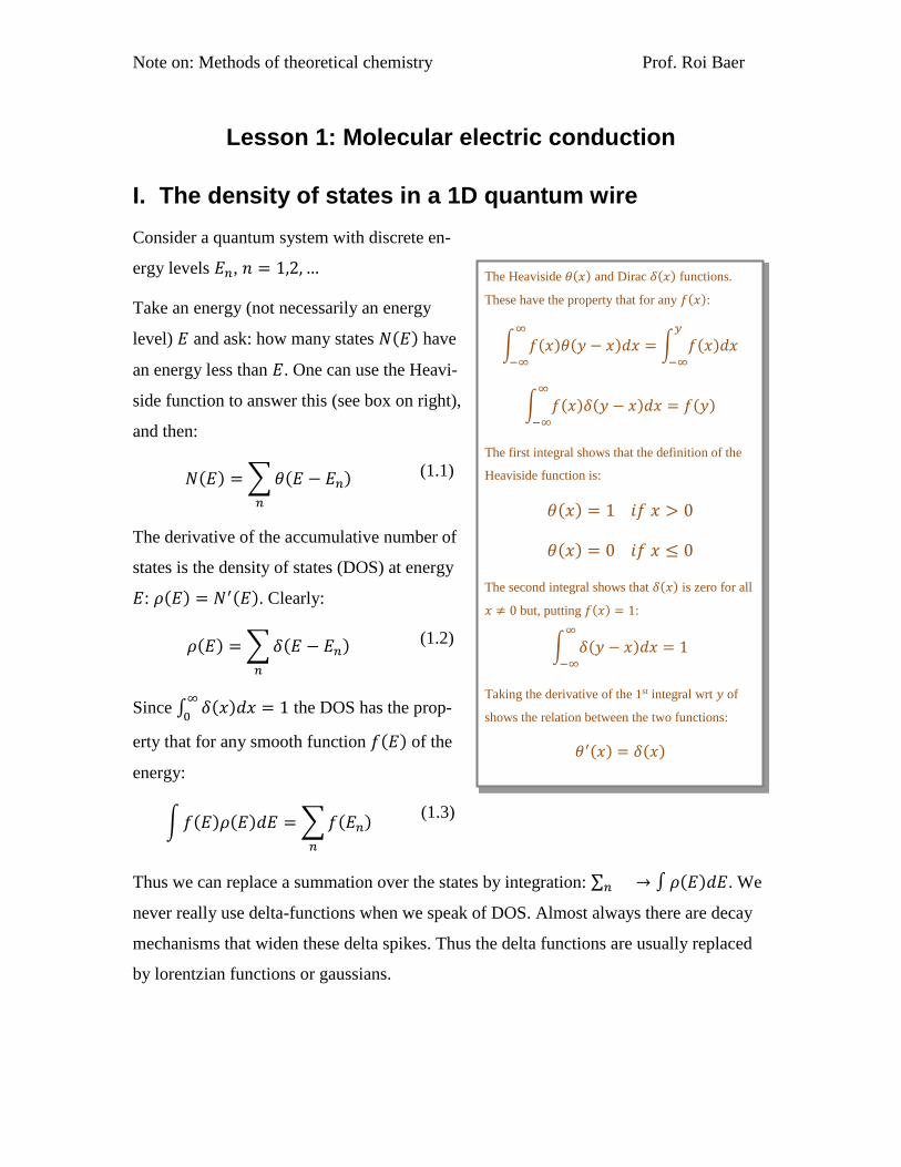
Take an energy (not necessarily an energy
level) 𝐸 and ask: how many states 𝑁(𝐸) have
an energy less than 𝐸. One can use the Heavi-
side function to answer this (see box on right),
and then:
𝑁(𝐸) = ∑ 𝜃(𝐸 − 𝐸𝑛)
𝑛
(1.1)
The derivative of the accumulative number of
states is the density of states (DOS) at energy
𝐸: 𝜌(𝐸) = 𝑁′(𝐸). Clearly:
𝜌(𝐸) = ∑ 𝛿(𝐸 − 𝐸𝑛)
𝑛
(1.2)
Since ∫ 𝛿(𝑥)𝑑𝑥∞
0= 1 the DOS has the prop-
erty that for any smooth function 𝑓(𝐸) of the
energy:
∫ 𝑓(𝐸)𝜌(𝐸)𝑑𝐸 = ∑ 𝑓(𝐸𝑛)
𝑛
(1.3)
Thus we can replace a summation over the states by integration: ∑𝑛 → ∫ 𝜌(𝐸)𝑑𝐸. We
never really use delta-functions when we speak of DOS. Almost always there are decay
mechanisms that widen these delta spikes. Thus the delta functions are usually replaced
by lorentzian functions or gaussians.
The Heaviside 𝜃(𝑥) and Dirac 𝛿(𝑥) functions.
These have the property that for any 𝑓(𝑥):
∫ 𝑓(𝑥)𝜃(𝑦 − 𝑥)𝑑𝑥∞
−∞
= ∫ 𝑓(𝑥)𝑑𝑥𝑦
−∞
∫ 𝑓(𝑥)𝛿(𝑦 − 𝑥)𝑑𝑥∞
−∞
= 𝑓(𝑦)
The first integral shows that the definition of the
Heaviside function is:
𝜃(𝑥) = 1 𝑖𝑓 𝑥 > 0
𝜃(𝑥) = 0 𝑖𝑓 𝑥 ≤ 0
The second integral shows that 𝛿(𝑥) is zero for all
𝑥 ≠ 0 but, putting 𝑓(𝑥) = 1:
∫ 𝛿(𝑦 − 𝑥)𝑑𝑥∞
−∞
= 1
Taking the derivative of the 1st integral wrt 𝑦 of
shows the relation between the two functions:
𝜃′(𝑥) = 𝛿(𝑥)
Note on: Methods of theoretical chemistry Prof. Roi Baer
Let us compute the DOS of an important basic system: a particle on a ring of circumfer-
ence 𝐿. As with any free particle the energy is 𝐸𝑚 =𝑝𝑚
2
2𝜇 where 𝑚 = 0, ±1, ±2, … and 𝑝𝑚
is the linear momentum of the particle corresponding to an angular momentum ℏ𝑚. For a
particle on a ring of radius 𝑎 the angular momentum 𝒓 × 𝒑 is simply 𝑎𝑝. Thus 𝑝𝑚 =
ℏ𝑚
𝐿/2𝜋= 𝑚
ℎ
𝐿. We see that the linear momentum 𝑝𝑚 = 𝑚 × Δ𝑝 is equally spaced where the
spacing is Δ𝑝 =ℎ
𝑚. Compute 𝑁(𝐸). We find the momentum corresponding to 𝐸:
𝑝(𝐸)2
2𝜇= 𝐸 → 𝑝(𝐸) = ±√2𝜇𝐸
And thus the number of states with energy less than 𝐸 is the number of states 𝑚 with
momentum 𝑝𝑚 in the interval −𝑝(𝐸) < 𝑝𝑚 < 𝑝(𝐸). So: 𝑁(𝐸) = 2 × 𝑚(𝐸) − 1 where
𝑚(𝐸) = [𝑝(𝐸)
Δ𝑝] and we use the notation that [𝑥] is the largest integer smaller than 𝑥. If we
think of a long wire, we can imagine that the integer aspect is smoothed out, so we can
write:
𝑁(𝐸) = 2𝐿𝑝(𝐸)
ℎ
The density of states is just the derivative of this. From 𝑝2 = 2𝜇𝐸, and taking derivative
w.r.t. 𝐸 we have 𝑝𝑝′ = 𝜇 so that: 𝜌(𝐸) = 𝑁′(𝐸). Thus, in terms of momentum:
𝜌(𝐸) = 2𝜇𝐿
ℎ𝑝(𝐸)
(1.4)
Note that the density of states is proportional to the length of the wire and inverse prop-
tional to the square root of the energy.
II. Theory of electric conduction through molecules
Consider an electron on the ring discussed above and ask: for a given state 𝑚 what is the
electric current? Since the velocity is 𝑣𝑚 =𝑝𝑚
𝜇, the time the electron completes a rotation
Note on: Methods of theoretical chemistry Prof. Roi Baer
is 𝜏𝑚 =𝐿
𝑣𝑚 and so 𝐼𝑚 =
𝑒
𝜏𝑚=
𝑒𝑣𝑚
𝐿=
𝑒𝑝𝑚
𝜇𝐿. For a long wire we can write these quantities as
functions of 𝐸
𝐼(𝐸) =𝑒
𝜇𝐿𝑝(𝐸) (2.1)
Now, let us try to connect the current and the density of states 𝜌. Using (1.4), we obtain a
relation between the current going left (say) and the density of states of the “wire”:
𝐼(𝐸)𝜌(𝐸) =𝑒
ℎ (2.2)
Note we “lost” a factor 2 because for each energy we consider only the “left” going
states. This relation is remarkable: when an electron is transported through an energy lev-
el 𝐸 of a device, the product of the current by the density of states is independent of 𝐸, of
the electron mass or the wire length! In fact the result is a constant of nature 𝑒
ℎ and is a
purely quantum effect (due to the presence of ℎ)! What does this inverse proportionality
of the current to the density of states mean? It means that wen you calculate the current
resulting from all energy levels in the interval Δ𝐸 Δ𝐸 = 𝐸2 − 𝐸1 then the current is the
simple result:
𝐼(𝐸2, 𝐸1) =𝑒
ℎ∫ 𝐼(𝐸)𝜌(𝐸)𝑑𝐸
𝐸2
𝐸1
=𝑒
ℎ(𝐸2 − 𝐸1) =
𝑒
ℎΔ𝐸
The total current of electrons in an energy range Δ𝐸 is just 𝑒
ℎΔ𝐸: indeed a remarkably
simple rule! This rule is now going to be used to compute the current in a molecular junc-
tion.
Now, consider a wire connected to two electrodes. We focus on “non-interacting elec-
trons”. This means that each electron is independent (except for Pauli principle) from
each other electron. The electrodes inject electrons into the wire and after the electron
passes through the wire it is absorbed by the electrodes. The total current in the wire is
the difference between currents going from the left to the right and from the right to the
left:
𝐼 = 𝐼𝐿→𝑅 − 𝐼𝑅→𝐿 (2.3)
Note on: Methods of theoretical chemistry Prof. Roi Baer
To get the current from left to right we have to sum over all states with positive momen-
tum: 𝐼𝐿→𝑅 = 2 ∑ 𝑤𝑛𝑖𝐿→𝑅𝑅 (𝐸𝑛)𝑛,𝑝>0 where 𝑛 enumerates the states in the left lead and
𝑖𝐿→𝑅𝑅 (𝐸𝑛) is the electric current in the right lead as a result of an impingement of an elec-
tron of energy 𝐸𝑛 coming from the left lead. Note that such an electron coming from the
left can either pass to the right side and contribute to 𝑖𝐿→𝑅𝑅 or to be reflected backwards.
Clearly there is a probability 𝑇(𝐸𝑛) that the impinging electron passes to the right. Be-
cause the number of electrons impinging on the wire coming from left is:
𝑖𝐿→𝑅𝑅 (𝐸) = 𝑤(𝐸)𝑇𝐿→𝑅(𝐸) (
𝑒
ℎ𝜌𝐿(𝐸))
𝑇𝐿→𝑅(𝐸) is a transmission coefficient. 𝑤(𝐸) is the joint probability that the left lead actu-
ally has an electron in state 𝑛 and that on the right the corresponding level of the same
energy is vacant (because of the Pauli principle, if the level is occupied the electron can-
not flow there since a level cannot be occupied by 2 electrons or more). The factor 2
comes from the two possible spin states. Clearly, because electrons are fermions the
population of levels is determined from the Fermi Dirac distributions in the two elec-
trodes, thus:
𝑤(𝐸) = 𝑓𝐿(𝐸)(1 − 𝑓𝑅(𝐸)) (2.4)
Where 𝑓𝑗(𝐸) =1
1+𝑒𝛽(𝐸−𝜇𝑗)
, 𝑗 = 𝐿, 𝑅 is the Fermi-Dirac distribution, 𝜇𝑗 is the chemical
potential of the left or right electrode and (𝑘𝐵𝛽)−1 is the temperature (𝑘𝐵 is Boltzmann’s
constant). All these give:
𝐼𝐿→𝑅 = 2 ∑ 𝑓𝐿(𝐸𝑛)(1 − 𝑓𝑅(𝐸𝑛))𝑖𝐿→𝑅𝑅 (𝐸𝑛)
𝑛,𝑝>0
= 2 ∫ 𝑓𝐿(𝐸)(1 − 𝑓𝑅(𝐸))𝑖𝐿→𝑅𝑅 (𝐸)𝜌𝐿(𝐸)𝑑𝐸
=2𝑒
ℎ∫ 𝑓𝐿(𝐸)(1 − 𝑓𝑅(𝐸))𝑇𝐿→𝑅(𝐸)𝑑𝐸
(2.5)
𝑇𝐿→𝑅(𝐸) is a transmission coefficient. It answers the question: what is the probability that
an electron of energy 𝐸 moving to the right in the left lead ends up in the right lead.
Posed this way, such a question is ill-defined, but it is intuitively clearer.

Note on: Methods of theoretical chemistry Prof. Roi Baer
A similar expression will be used for 𝐼𝑅→𝐿. Thus
𝐼𝑅→𝐿 =2𝑒
ℎ∫ 𝑓𝑅(𝐸)(1 − 𝑓𝐿(𝐸))𝑇𝑅→𝐿(𝐸)𝑑𝐸
(2.6)
We will show in the next section that 𝑇𝑅→𝐿(𝐸) = 𝑇𝐿→𝑅(𝐸) and we thus call both “the
transmission coefficient” 𝑇(𝐸). From Eq. (2.3) we then find:
𝐼 =2𝑒
ℎ∫[𝑓(𝐸 − 𝜇𝐿) − 𝑓(𝐸 − 𝜇𝑅)]𝑇(𝐸)𝑑𝐸
(2.7)
This is Landauer’s equation for the current in a junction. It is very simple. The electronic
structure of the leads and the constriction go in only through the transmission coefficient.
At zero temperature, with no barriers (𝑇(𝐸) = 1) we get the almost similar rule as we
had above:
𝐼 =2𝑒
ℎ(𝜇𝐿 − 𝜇𝑅) =
2𝑒2
ℎΔ𝑉
(2.8)
Where Δ𝑉 = 𝑒−1(𝜇𝐿 − 𝜇𝑅) is the voltage bias between the two electrodes. The conduct-
ance is the derivative of the current by the bias. The conductance in the above case is thus
𝐺 =𝑑𝐼
𝑑Δ𝑉=
2𝑒2
ℎ.
III. 1D model of a molecular junction
We now build a model for a molecular junction. In the junction there are 3 entities: the
molecule, and the left/right metallic leads. Our model will assume that electrons are non-
interacting. This may sound strange, since electrons interact quite strongly, however, it is
well known that a good approximation for the behavior of electronic systems is that by
modifying the overall potential suitably they can be approximately assumed to be non-
interacting. In some phenomena interactions are extremely important, however, such
phenomena are beyond the scope of our treatment.
The model for the molecule is a well, for the present we will assume a square well, but
the methods we develop below are suitable for any shape. So our molecule is schemati-
cally shown in this diagram:
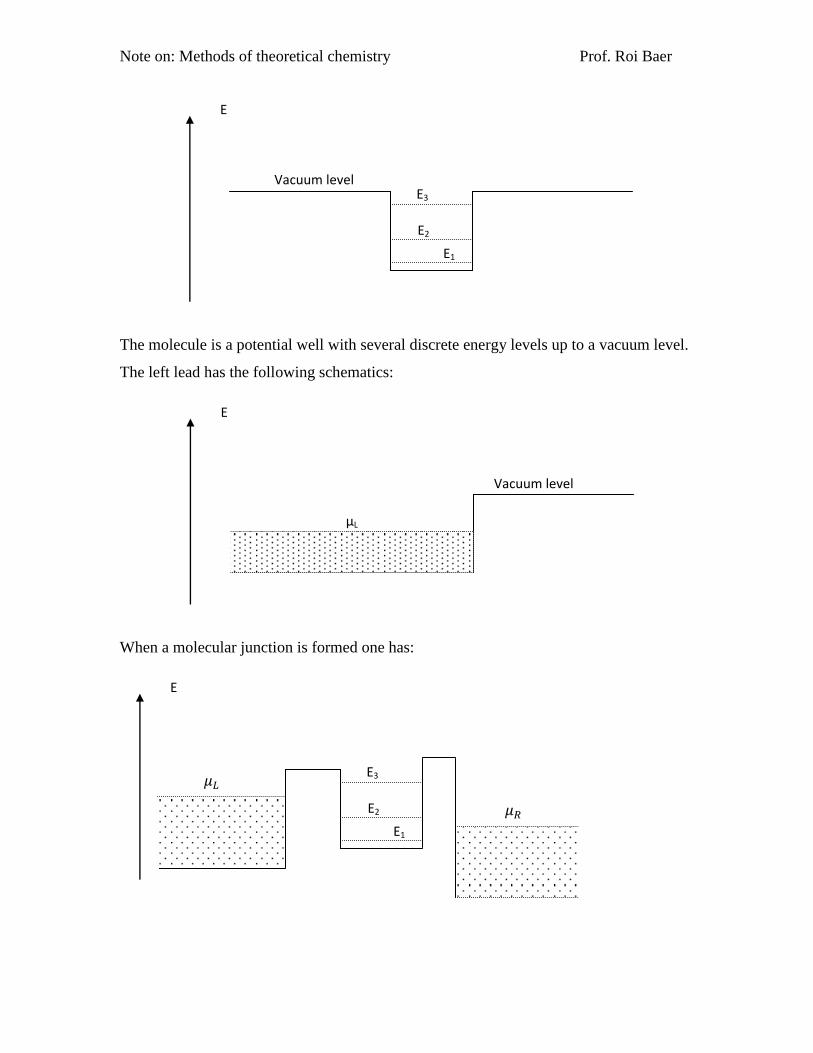
Note on: Methods of theoretical chemistry Prof. Roi Baer
The molecule is a potential well with several discrete energy levels up to a vacuum level.
The left lead has the following schematics:
When a molecular junction is formed one has:
E
Vacuum level
E1
E2
E3
E
Vacuum level
μL
E
E1
E2
E3 𝜇𝐿
𝜇𝑅

Note on: Methods of theoretical chemistry Prof. Roi Baer
Due to the double barrier tunneling phenomenon, we will discuss in the next section, one
can think of conduction as "going through" the energy levels of the molecule (this is a
good assumption when the molecule is weakly coupled to the metal). At zero temperature
one can see in the figure that conductance through molecular level 1 is impossible since
the corresponding energy levels on both sides are occupied (the Fermi-Dirac difference
terms at this energy give zero). In fact due to this, this level of the molecule will itself be
occupied by 2 electrons. I say it is nearly impossible because one can still imagine a pro-
cess in which one electron in level 1 of the molecule will jump up in energy to the lowest
unoccupied state of the right lead (energy 𝜇𝑅) and an electron from the left lead at the
same energy will replace it. But as we shall see in calculations such events have very
small probability since they are essentially tunneling events (violate the energy conserva-
tion for a short period of time). Conduction through level 3 is also nearly impossible for
the same but opposite reason: there are no electrons of energy 𝐸3 in the metals and thus
conductance will occur only through tunneling which has a small probability. However
conduction may occur more readily through level 2 since the left lead can supply elec-
trons that go through the molecule and come out in the vacant levels of the right lead.
IV. Calculating T(E): Transfer Matrix Method
In order to estimate the conductance we need a way to compute the transmission coeffi-
cient in the Landauer formula 𝑇(𝐸). We develop such a method, for 1D systems now.
Consider a potential step, going from potential 𝑉𝐿, 𝑉𝑅 at 𝑥 = 𝑎. The wave functions with
energy 𝐸 on the left and right side of this point are:
𝜓𝐿(𝑟) = 𝐿+𝑒𝑖𝑘𝑟 + 𝐿−𝑒−𝑖𝑘𝑟 𝜓𝐿′ (𝑟) = 𝑖𝑘(𝐿+𝑒𝑖𝑘𝑟 − 𝐿−𝑒−𝑖𝑘𝑟) (3.1)
𝜓𝑅(𝑟) = 𝑅+𝑒𝑖𝑞𝑟 + 𝑅−𝑒−𝑖𝑞𝑟 𝜓𝑅′ (𝑟) = 𝑖𝑞(𝑅+𝑒𝑖𝑞𝑟 − 𝑅−𝑒−𝑖𝑞𝑟) (3.2)
Where ℏ2𝑘2
2𝜇= 𝐸 − 𝑉𝐿,
2 2
2R
qE V . 𝜓𝐿(𝑟) is composed of two states with exact mo-
mentum 𝑘: one going to the right with amplitude 𝐿+ and the other goinf to the left, with
amplitude 𝐿−. Similarly, the other wave functions.
Note on: Methods of theoretical chemistry Prof. Roi Baer
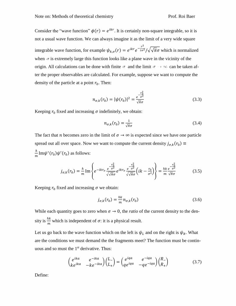
Consider the “wave function” 𝜙(𝑟) = 𝑒𝑖𝑘𝑟. It is certainly non-square integrable, so it is
not a usual wave function. We can always imagine it as the limit of a very wide square
integrable wave function, for example 𝜓𝑘,𝜎(𝑟) = 𝑒𝑖𝑘𝑟𝑒−
𝑟2
2𝜎2/√√𝜋𝜎 which is normalized
when is extremely large this function looks like a plane wave in the vicinity of the
origin. All calculations can be done with finite and the limit can be taken af-
ter the proper observables are calculated. For example, suppose we want to compute the
density of the particle at a point 𝑟0. Then:
𝑛𝜎,𝑘(𝑟0) = |𝜓(𝑟0)|2 =𝑒
−𝑟0
2
𝜎2
√𝜋𝜎 (3.3)
Keeping 𝑟0 fixed and increasing 𝜎 indefinitely, we obtain:
𝑛𝜎,𝑘(𝑟0) =1
√𝜋𝜎 (3.4)
The fact that 𝑛 becomes zero in the limit of 𝜎 → ∞ is expected since we have one particle
spread out all over space. Now we want to compute the current density 𝑗𝜎,𝑘(𝑟0) ≡
ℏ
𝑚Im𝜓∗(𝑟0)𝜓′(𝑟0) as follows:
𝑗𝜎,𝑘(𝑟0) =ℏ
𝑚Im {𝑒−𝑖𝑘𝑟𝑜
𝑒−
𝑟02
𝜎2
√√𝜋𝜎𝑒𝑖𝑘𝑟𝑜
𝑒−
𝑟02
𝜎2
√√𝜋𝜎(𝑖𝑘 −
𝑟0
𝜎2)} =ℏ𝑘
𝑚
𝑒−
𝑟02
𝜎2
√𝜋𝜎 (3.5)
Keeping 𝑟0 fixed and increasing 𝜎 we obtain:
𝑗𝜎,𝑘(𝑟0) =ℏ𝑘
𝑚𝑛𝜎,𝑘(𝑟0) (3.6)
While each quantity goes to zero when 𝜎 → 0, the ratio of the current density to the den-
sity is ℏ𝑘
𝑚 which is independent of 𝜎: it is a physical result.
Let us go back to the wave function which on the left is 𝜓𝐿 and on the right is 𝜓𝑅. What
are the conditions we must demand the the fragments meet? The function must be contin-
uous and so must the 1st derivative. Thus:
( 𝑒𝑖𝑘𝑎 𝑒−𝑖𝑘𝑎
𝑘𝑒𝑖𝑘𝑎 −𝑘𝑒−𝑖𝑘𝑎) (
𝐿−
𝐿+) = (
𝑒𝑖𝑞𝑎 𝑒−𝑖𝑞𝑎
𝑞𝑒𝑖𝑞𝑎 −𝑞𝑒−𝑖𝑞𝑎) (𝑅−
𝑅+) (3.7)
Define:

Note on: Methods of theoretical chemistry Prof. Roi Baer
𝑀(𝑎; 𝑘 → 𝑞) = (𝑒𝑖𝑞𝑎 𝑒−𝑖𝑞𝑎
𝑞𝑒𝑖𝑞𝑎 −𝑞𝑒−𝑖𝑞𝑎)−1
( 𝑒𝑖𝑘𝑎 𝑒−𝑖𝑘𝑎
𝑘𝑒𝑖𝑘𝑎 −𝑘𝑒−𝑖𝑘𝑎) (3.8)
And so:
𝑀(𝑎; 𝑘 → 𝑞) (𝐿−
𝐿+) = (
𝑅−
𝑅+) (3.9)
𝑀(𝑎; 𝑘 → 𝑞) is the transfer matrix. It determines the way the wave with wave-number 𝑘
interacts with the interface at 𝑎, after which the wave must have wave-number 𝑞. Note
that:
(𝑒𝑖𝑞𝑎 𝑒−𝑖𝑞𝑎
𝑞𝑒𝑖𝑞𝑎 −𝑞𝑒−𝑖𝑞𝑎)−1
=1
2𝑞(
𝑞𝑒−𝑖𝑞𝑎 𝑒−𝑖𝑞𝑎
𝑞𝑒𝑖𝑞𝑎 −𝑒𝑖𝑞𝑎) (3.10)
Thus, 𝑀(𝑎; 𝑘 → 𝑞) =1
2𝑞(
𝑞𝑒−𝑖𝑞𝑎 𝑒−𝑖𝑞𝑎
𝑞𝑒𝑖𝑞𝑎 −𝑒𝑖𝑞𝑎) ( 𝑒𝑖𝑘𝑎 𝑒−𝑖𝑘𝑎
𝑘𝑒𝑖𝑘𝑎 −𝑘𝑒−𝑖𝑘𝑎) and:
𝑀(𝑎; 𝑘 → 𝑞) =1
2𝑞(
(𝑞 + 𝑘)𝑒𝑖(𝑘−𝑞)𝑎 (𝑞 − 𝑘)𝑒−𝑖(𝑘+𝑞)𝑎
(𝑞 − 𝑘)𝑒𝑖(𝑘+𝑞)𝑎 (𝑞 + 𝑘)𝑒−𝑖(𝑘−𝑞)𝑎) (3.11)
The transfer matrix can be used as in "Lego-land": You simply calculate the matrix at
each junction and then multiply them. For example, a wave hitting two consecutive inter-
faces. One at 𝑎1 and the other at 𝑎2. The potential at left is 𝑉0, after 𝑎1 it is 𝑉1 and after
𝑎2 it is 𝑉2. Then the TM of the entire "device" is:
𝑀 = 𝑀(𝑎2; 𝑞1 → 𝑞2)𝑀(𝑎1; 𝑞0 → 𝑞1) (3.12)
To calculate the probability to transfer from left to right, we impose the boundary condi-
tions that we have an incoming wave from left (amplitude 1) and an outgoing wave from
the right. There is no incoming wave from the right thus: 𝑅− = 0. There may be a reflect-
ed wave, of amplitude 𝐿−. Thus the scattering is described by:
𝑀 (1
𝐿−) = (
𝑅+
0)
(3.13)
There are 2 equations with 2 unknowns. After rearrangement, we get:
(𝑀11 + 𝑀12𝐿−
𝑀21 + 𝑀22𝐿−) = (
𝑅+
0)
(3.14)
From the second equation the 𝐿_ amplitude is:
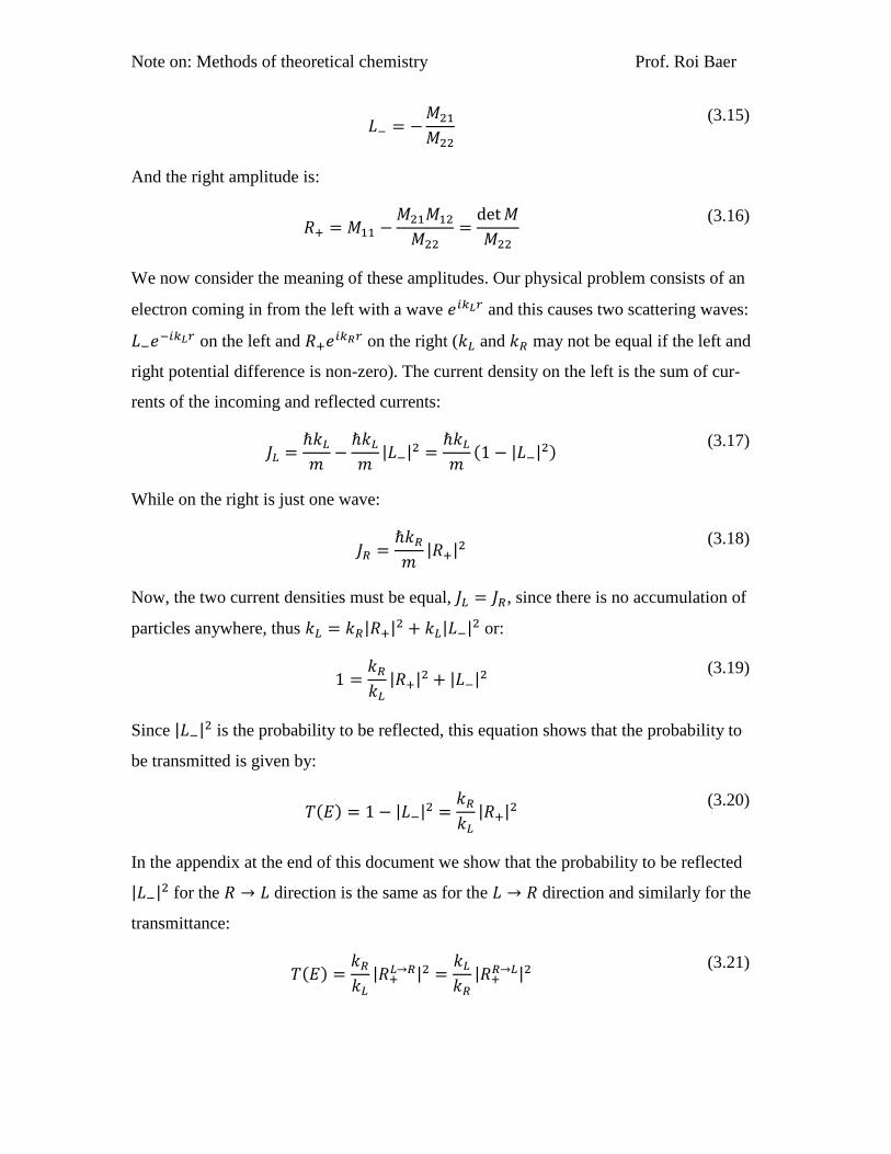
Note on: Methods of theoretical chemistry Prof. Roi Baer
𝐿− = −𝑀21
𝑀22
(3.15)
And the right amplitude is:
𝑅+ = 𝑀11 −𝑀21𝑀12
𝑀22=
det 𝑀
𝑀22
(3.16)
We now consider the meaning of these amplitudes. Our physical problem consists of an
electron coming in from the left with a wave 𝑒𝑖𝑘𝐿𝑟 and this causes two scattering waves:
𝐿−𝑒−𝑖𝑘𝐿𝑟 on the left and 𝑅+𝑒𝑖𝑘𝑅𝑟 on the right (𝑘𝐿 and 𝑘𝑅 may not be equal if the left and
right potential difference is non-zero). The current density on the left is the sum of cur-
rents of the incoming and reflected currents:
𝐽𝐿 =ℏ𝑘𝐿
𝑚−
ℏ𝑘𝐿
𝑚|𝐿−|2 =
ℏ𝑘𝐿
𝑚(1 − |𝐿−|2)
(3.17)
While on the right is just one wave:
𝐽𝑅 =ℏ𝑘𝑅
𝑚|𝑅+|2
(3.18)
Now, the two current densities must be equal, 𝐽𝐿 = 𝐽𝑅, since there is no accumulation of
particles anywhere, thus 𝑘𝐿 = 𝑘𝑅|𝑅+|2 + 𝑘𝐿|𝐿−|2 or:
1 =𝑘𝑅
𝑘𝐿
|𝑅+|2 + |𝐿−|2 (3.19)
Since |𝐿−|2 is the probability to be reflected, this equation shows that the probability to
be transmitted is given by:
𝑇(𝐸) = 1 − |𝐿−|2 =𝑘𝑅
𝑘𝐿
|𝑅+|2 (3.20)
In the appendix at the end of this document we show that the probability to be reflected
|𝐿−|2 for the 𝑅 → 𝐿 direction is the same as for the 𝐿 → 𝑅 direction and similarly for the
transmittance:
𝑇(𝐸) =𝑘𝑅
𝑘𝐿
|𝑅+𝐿→𝑅|2 =
𝑘𝐿
𝑘𝑅
|𝑅+𝑅→𝐿|2
(3.21)

Note on: Methods of theoretical chemistry Prof. Roi Baer
V. Numerical Integration
We want to discuss the way to compute a controlled approximation to the definite inte-
gral of a function 𝑓(𝑥):
𝐼(𝑓) = ∫ 𝑓(𝑥)𝑑𝑥𝑏
𝑎
(4.1)
Formulas which give approximations that can be used for any function are called a quad-
rature rule. To be controlled, they must give an estimate for the error.
A. The Rectangle Rule
The simplest way to perform numerical integration 𝐼(𝑓) is to divide the interval [𝑎, 𝑏] to
many (large 𝑁) equally spaced intervals, with spacing ℎ =𝑏−𝑎
𝑁:
𝑎 = 𝑥0, 𝑥𝑛+1 = 𝑥𝑛 + ℎ, 𝑥𝑁 = 𝑏 (4.2)
And then:
𝐼(𝑓) ≈ ∑ 𝑓𝑛ℎ
𝑁−1
𝑛=0
= (𝑓0 + 𝑓1 + ⋯ 𝑓𝑁−1)ℎ
(4.3)
(we use: 𝑓𝑛 ≡ 𝑓(𝑥𝑛)). The error associated with this procedure can be estimated using
Taylor expansion to first order:
𝐼(𝑓) = ∫ 𝑓(𝑥)𝑑𝑥𝑏
𝑎
= ∑ ∫ 𝑓(𝑥)𝑑𝑥𝑥𝑛+1
𝑥𝑛
𝑁−1
𝑛=0
= ∑ ∫ (𝑓(𝑥𝑛) + 𝑂(ℎ))𝑑𝑥𝑥𝑛+1
𝑥𝑛
𝑁−1
𝑛=0
= ∑ 𝑓𝑛
𝑁−1
𝑛=0
ℎ + 𝑂(ℎ2)𝑁 = ∑ 𝑓𝑛
𝑁−1
𝑛=0
ℎ + 𝑂(ℎ)
(4.4)
Thus, when N is increased 2 fold, making the use of (4.3) twice as expensive, the error is
decreased by a factor of 2. This is a first order formula.
B. The Trapeze Rule
There is a simple way to improve. For 𝑥 ∈ [𝑥𝑛, 𝑥𝑛+1]. Instead of using the Taylor expan-
sion to first 𝑓(𝑥) = 𝑓𝑛 + 𝑂(ℎ). Let us use it to second order:
Note on: Methods of theoretical chemistry Prof. Roi Baer
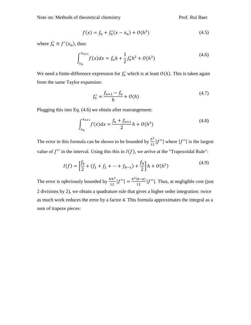
𝑓(𝑥) = 𝑓𝑛 + 𝑓𝑛′(𝑥 − 𝑥𝑛) + 𝑂(ℎ2) (4.5)
where 𝑓𝑛′ ≡ 𝑓′(𝑥𝑛), thus:
∫ 𝑓(𝑥)𝑑𝑥𝑥𝑛+1
𝑥𝑛
= 𝑓𝑛ℎ +1
2𝑓𝑛
′ℎ2 + 𝑂(ℎ3) (4.6)
We need a finite-difference expression for 𝑓𝑛′ which is at least 𝑂(ℎ). This is taken again
from the same Taylor expansion:
𝑓𝑛′ =
𝑓𝑛+1 − 𝑓𝑛
ℎ+ 𝑂(ℎ)
(4.7)
Plugging this into Eq. (4.6) we obtain after rearrangement:
∫ 𝑓(𝑥)𝑑𝑥𝑥𝑛+1
𝑥𝑛
=𝑓𝑛 + 𝑓𝑛+1
2ℎ + 𝑂(ℎ3)
(4.8)
The error in this formula can be shown to be bounded by ℎ3
12|𝑓′′| where |𝑓′′| is the largest
value of 𝑓′′ in the interval. Using this this in 𝐼(𝑓), we arrive at the "Trapezoidal Rule":
𝐼(𝑓) = [𝑓0
2+ (𝑓1 + 𝑓2 + ⋯ + 𝑓𝑁−1) +
𝑓𝑁
2] ℎ + 𝑂(ℎ2)
(4.9)
The error is opbviously bounded by 𝑁ℎ3
12|𝑓′′| =
ℎ2(𝑏−𝑎)
12|𝑓′′|. Thus, at negligible cost (just
2 divisions by 2), we obtain a quadrature rule that gives a higher order integration: twice
as much work reduces the error by a factor 4. This formula approximates the integral as a
sum of trapeze pieces:
Note on: Methods of theoretical chemistry Prof. Roi Baer
a
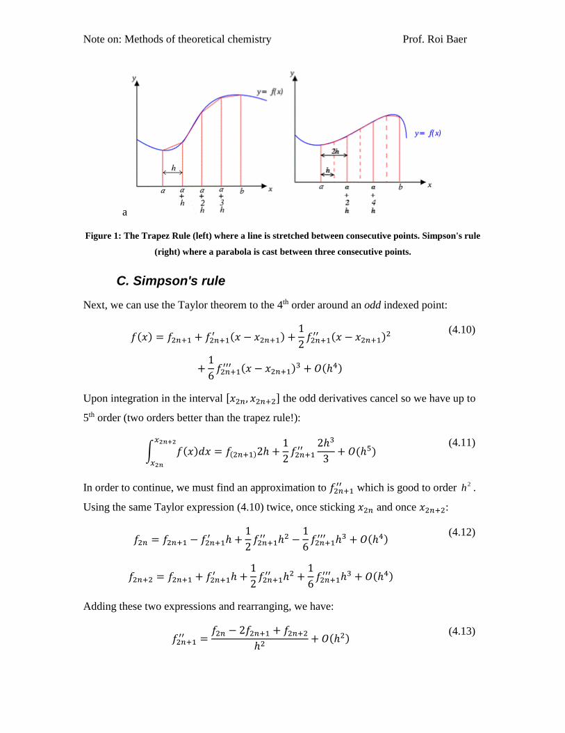
Figure 1: The Trapez Rule (left) where a line is stretched between consecutive points. Simpson's rule
(right) where a parabola is cast between three consecutive points.
C. Simpson's rule
Next, we can use the Taylor theorem to the 4th order around an odd indexed point:
𝑓(𝑥) = 𝑓2𝑛+1 + 𝑓2𝑛+1′ (𝑥 − 𝑥2𝑛+1) +
1
2𝑓2𝑛+1
′′ (𝑥 − 𝑥2𝑛+1)2
+1
6𝑓2𝑛+1
′′′ (𝑥 − 𝑥2𝑛+1)3 + 𝑂(ℎ4)
(4.10)
Upon integration in the interval [𝑥2𝑛, 𝑥2𝑛+2] the odd derivatives cancel so we have up to
5th order (two orders better than the trapez rule!):
∫ 𝑓(𝑥)𝑑𝑥𝑥2𝑛+2
𝑥2𝑛
= 𝑓(2𝑛+1)2ℎ +1
2𝑓2𝑛+1
′′2ℎ3
3+ 𝑂(ℎ5)
(4.11)
In order to continue, we must find an approximation to 𝑓2𝑛+1′′ which is good to order 2
h .
Using the same Taylor expression (4.10) twice, once sticking 𝑥2𝑛 and once 𝑥2𝑛+2:
𝑓2𝑛 = 𝑓2𝑛+1 − 𝑓2𝑛+1′ ℎ +
1
2𝑓2𝑛+1
′′ ℎ2 −1
6𝑓2𝑛+1
′′′ ℎ3 + 𝑂(ℎ4)
𝑓2𝑛+2 = 𝑓2𝑛+1 + 𝑓2𝑛+1′ ℎ +
1
2𝑓2𝑛+1
′′ ℎ2 +1
6𝑓2𝑛+1
′′′ ℎ3 + 𝑂(ℎ4)
(4.12)
Adding these two expressions and rearranging, we have:
𝑓2𝑛+1′′ =
𝑓2𝑛 − 2𝑓2𝑛+1 + 𝑓2𝑛+2
ℎ2+ 𝑂(ℎ2)
(4.13)

Note on: Methods of theoretical chemistry Prof. Roi Baer
Plugging into Eq. (4.11) and rearranging gives:
∫ 𝑓(𝑥)𝑑𝑥𝑥2𝑛+2
𝑥2𝑛
= (𝑓2𝑛 + 4𝑓(2𝑛+1) + 𝑓2𝑛+2)ℎ
3+ 𝑂(ℎ5)
(4.14)
In this case, the error term is bounded by (2ℎ)5
2880|𝑓′′′| =
ℎ5
90|𝑓′′′|. Summing over 𝑛, and as-
suming 𝑁 is even (𝑁 = 2𝑀) we have Simpson's rule:
𝐼(𝑓) = ∑ ∫ 𝑓(𝑥)𝑑𝑥𝑥2𝑛+2
𝑥2𝑛
𝑀−1
𝑛=0
= ∑ (𝑓2𝑛 + 4𝑓(2𝑛+1) + 𝑓2𝑛+2)
𝑀−1
𝑛=0
ℎ
3+ 𝑂(ℎ4)
= [(𝑓0 + 4𝑓1 + 𝑓2) + (𝑓2 + 4𝑓3 + 𝑓4) + ⋯ ]ℎ
3+ 𝑂(ℎ4)
= [𝑓0 + 4𝑓1 + 2𝑓2 + 4𝑓3 + 2𝑓4 + ⋯ ]ℎ
3+ 𝑂(ℎ4)
(4.15)
Thus, Simpson's rule is:
𝐼(𝑓) = [𝑓0 + 4 ∑ 𝑓2𝑛−1
𝑀
𝑛=1
+ 2 ∑ 𝑓2𝑛
𝑀−1
𝑛=1
+ 𝑓2𝑀]ℎ
3+ 𝑂(ℎ4)
(4.16)
With minute amount of additional work we obtain a much higher degree of approxima-
tion. Now, increasing work by a factor of two improves the accuracy by a factor 16.
One can continue this procedure to higher orders, but one has to always make sure that
the Nth derivatives of the integrand do not grow faster than the order of the method. Since
on computer we have finite arithmetic, numerical noise grows as you take higher and
higher order derivatives.
Going one step further in this analysis gives Boole’s rule:
𝐼(𝑓) = [7𝑓0 + 32 ∑ 𝑓4𝑛−3
𝑀
𝑛=1
+ 12 ∑ 𝑓4𝑛−2
𝑀
𝑛=1
+ 32 ∑ 𝑓4𝑛−1
𝑀
𝑛=1
+ 14 ∑ 𝑓4𝑛
𝑀−1
𝑛=1
+ 7𝑓4𝑀]ℎ
90+ 𝑂(ℎ6)
(4.17)

Note on: Methods of theoretical chemistry Prof. Roi Baer
VI. Appendix:
Notice also that for a particle coming in from the opposite side the same method will in-
volve instead of 𝑀(𝑎1, 𝑘1 → 𝑘2)𝑀(𝑎0, 𝑘0 → 𝑘1) the following matrix product:
𝑀(−𝑎0, 𝑘1 → 𝑘0)𝑀(−𝑎2, 𝑘2 → 𝑘1) (just redraw the junction using a mirror image). No-
tice the following:
𝑀(𝑎; 𝑘 → 𝑞) =1
2𝑞(
(𝑞 + 𝑘)𝑒𝑖(𝑘−𝑞)𝑎 (𝑞 − 𝑘)𝑒−𝑖(𝑘+𝑞)𝑎
(𝑞 − 𝑘)𝑒𝑖(𝑘+𝑞)𝑎 (𝑞 + 𝑘)𝑒−𝑖(𝑘−𝑞)𝑎)
𝑀(−𝑎; 𝑞 → 𝑘) =1
2𝑘(
(𝑞 + 𝑘)𝑒𝑖(𝑘−𝑞)𝑎 −(𝑞 − 𝑘)𝑒𝑖(𝑘+𝑞)𝑎
−(𝑞 − 𝑘)𝑒−𝑖(𝑘+𝑞)𝑎 (𝑞 + 𝑘)𝑒−𝑖(𝑘−𝑞)𝑎)
(4.18)
Note the special structure of the 𝑀 matrices:
𝑀(𝑎, 𝑘 → 𝑞) =1
2𝑞(
𝐴 𝐵𝐵∗ 𝐴∗)
(4.19)
When one multiplies two matrices one obtains:
(𝐴 𝐵𝐵∗ 𝐴∗) (
𝐶 𝐷𝐷∗ 𝐶∗) = (
𝐴𝐶 + 𝐵𝐷∗ 𝐴𝐷 + 𝐵𝐶∗
𝐵∗𝐶 + 𝐴∗𝐷∗ 𝐵∗𝐷 + 𝐴∗𝐶∗) (4.20)
The product is also of the same structure. These then form a group. The mirror change
moves from:
(𝐴 𝐵𝐵∗ 𝐴∗) → (
𝐴 −𝐵∗
−𝐵 𝐴∗ ) (4.21)
We define a “mirror of a matrix”:
(𝐴 𝐵𝐵∗ 𝐴∗)
𝑀
= (𝐴 −𝐵∗
−𝐵 𝐴∗ ) (4.22)
Clearly (𝑄𝑀)𝑀 = 𝑄. It is easy to check that:
(𝑃𝑄)𝑀 = 𝑄𝑀𝑃𝑀 (4.23)
One further easily sees that
det 𝑄 = det 𝑄𝑀
𝑄11 = (𝑄𝑀)11 𝑄22 = (𝑄𝑀)22
(4.24)
From this we have:

Note on: Methods of theoretical chemistry Prof. Roi Baer
𝑀(𝑎, 𝑘 → 𝑞) =1
2𝑞(
𝐴 𝐵𝐵∗ 𝐴∗)
𝑀(−𝑎, 𝑞 → 𝑘) =1
2𝑘(
𝐴 𝐵𝐵∗ 𝐴∗)
𝑀
=𝑞
𝑘𝑀(𝑎, 𝑘 → 𝑞)𝑀
(4.25)
We thus have that the total TM of the mirror obeys:
𝑀𝑅→𝐿 =𝑘𝑅
𝑘𝐿
(𝑀𝐿→𝑅)𝑀 (4.26)
Thus one sees that the mirror barrier has:
𝑅+𝑀 =
𝑘𝑅
𝑘𝐿𝑅+ 𝐿−
𝑀 =𝑀12
M22= −𝐿−
(4.27)
Thus:
(𝑘𝐿
𝑘𝑅) |𝑅+
𝑀|2 = (𝑘𝑅
𝑘𝐿) |𝑅+|2 𝐿−
𝑀 =𝑀12
M22= −𝐿−
(4.28)