A

Helm ut lerchs"'Ma nager of Scientific Services, Mantreal Datacentre, lnternational Business Machin es

Ca. Ltd.,

lngo F. Grossma nnManager ,Management Science Applications, lnternatianal Business Machines

Co. Ltd .

Optimum Design of

Open-Pit Mines

Joint C.O.R.S. ond O.R.S.A. Conference,

Montreal , Moy 27-29, 1964

Tronsoct ions, C. l .M .,_ Vol ume LXV I I I , 1965, pp. 17-24

ABSTRACT

An open-pit mining operation can be .vieed ª:' a process by which the 01>en surface of a mme is contmuously deformed. The planning of a minin g program in rnlves the design of the final shape of this open surface. The approach de,·eloped in this paper is b:ised. on he follow ing assum ptions: l. the ty 1> of material, it nune,·aJue and its extraction cost is g1ven for each pomt; 2. restrictions on the geometry of the pit are specified (sur face bound aries and maximu m allowable wa ll slopes) ;

3. the objective is to maxim ize total profit - total mine value of material extracted minus total extraction

cost.Two numeric methods are proposed : .A sim ple

dynamic programming algorithm for the two-dimensional pit (or a single vertical section of a m ine), and. a moe elab?rate graph algorith m for the general three-d1mens1onal p1t.

lntrod uction

SURFACE mi ning prog ram is a complex opera tion that may extend over many years, and

in volve h uge capital expend i tu res and risk. Before un dertaking such an operation, it must be known

what ore there is to be mi ned ( types, grades, quantities and spatial d istribution ) ancl how much

of the oreshou ld be m ined to make the operation profitable.

The reserves of ore and i ts spatial distribution are estimated by geological i nterpretation of the informa tion obtai ned from d rill cores. The object of pit de sign then is to determine the amou nt of ore to be mi ned.

Assumi ng that the concentration of ores and im purities is known at each point, the problem is to de cide what the ultimate contour of the pit will be and in what stages this contou r is to be reached . Let us note that if, with respect to the global objectives of a mining program, an optimum pit contour exists, and if the mi ning operation is to be optimized, then this contour must be known, if only to minimize the total cost of mining.

•Now Senior Resea1·ch Mathematician, General Motors

Research Laboratory, Wanen, Mich.

Bulletin for January, 1965. Montreal

Open-Pit Model

Besides pit design, planning may bear on questions such as:

- what ma rket to select ;what u pgrad ing plants to install ;

- what quanti ties to extract, as a function of time;

- what mi ni ng methocls to use;- what transportation facili ties to provide.There is an in ti mate relationsh ip between al! the above

points, and it is meani ngless to consider any one component of pla nni ng separately. A mathema tical model taki ng i n to account al! possible alterna tives simu ltaneously wou ld, however, be of formidable size ancl its solu t ion wou ld be beyond the means of present knowhow. The model proposed in this paper will serve to explore alternatives in pit design, given a real or a hypothetical economical environment (market si tuation, plant configu ration, etc.). This en vironment is d escri bed by the mine value of ali ores present and the extraction cost of ores and waste materials. The obj ective then is to design the contour of a pit so as to maximize the d ifference between the total mine val ue of ore extrncted and the total extrac tion cost of ore and waste. The sote restrictions con cern the geometry of the pi t ; the wall slopes of the pit m ust not exceed certai n given angles that may vary with the depth of the pit or with the material.

Analytically, we can express the problem as follows: Let v, e and m be three density functions def ined at each point of a three-dimensional space.

v (x. y, z) = mine \"alue of ore per unit volume c(x. y, z) - extraction cost per unit volumem (x. y, z) v(x, y, z) -c(x, y, z) = pro'it per unit \ olume.

Let a (x, y, z) define an angle at each point and !et S be the family of surfaces such that at no point does their slope, with respect to a fixed horizontal plane, exceed a.

Let V be the fam ily of vol umes corresponding to the family, S, of surfaces. The problem is to find, among ali volum es, V, one that maximizes the integral

f.m(x, y, z) dx dy dz

47

Two-Dimensional Pit

Let us select the units u, and ui of a rectangular grid system such that

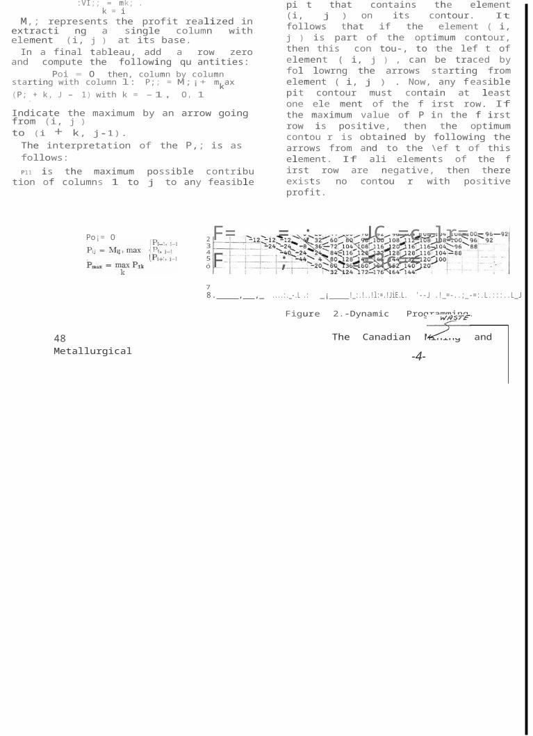
= tan aUj

For each unit rectangle (i, j ) determine the quan tity m 1i = v,J - C;;. Construct a new tableau (Fig ure 2) with the quantities

Figure l.

Generally, there is no simple analytical representa tion for the functions v and e; consequently, numeric methods must be used. The traditional approach is to divide the whole pit into parallel vertical sections, and to consider each section as a two-dimensional pit. The technique used to determine the contour of a section consists in moving three straight Jines, rep resenting the bottorn of the pit and two walls, at slopes a (see Figu re 1), and in evaluating the ore and the extraction cost of materials limited by the three lines. The conf igu ration of lines yielding the best re sults is then selected. (Here, a i s taken to be constant over the entire pit ) .

The following dynamic programming technique is simpler, faster and more accu rate.

a = 45°ffi¡j = V¡; - Cil

M;; = 1: mk,k = I

:VI;; = mk; .k = i

M,; represents the profit realized in extracti ng a single column with element (i, j ) at its base.

In a final tableau, add a row zero and compute the following qu antities:

Poi = O then, column by column starting with column l: P;; = M;¡+ mkax (P;.+ k, J - 1) with k = -1' O' 1

Indicate the maximum by an arrow going from (i, j )to (i + k, j-1).

The interpretation of the P,; is as follows:P11 is the maximum possible contribu tion of columns

1 to j to any feasible pi t that contains the element (i, j ) on its contour. It follows that if the element ( i, j ) is part of the optimum contour, then this con tou-, to the lef t of element ( i, j ) , can be traced by fol lowrng the arrows starting from element ( i, j ) . Now, any f easible pit contour must contain at least one ele ment of the f irst row. If the maximum value of P in the f irst row is positive, then the optimum contou r is obtained by following the arrows from and to the \ef t of this element. If ali elements of the f irst row are negative, then there exists no contou r with positive profit.

2345ó 78. , ,_ ....:._-.L .: _¡ !_:.!..!l:=.!JiE.L. '--J .!_=-..;_-=:.L.:::..L_J

Figure 2.-Dynamic Programming.

Oi'?E

-4-

Po¡= O JC =c ]r= =3c==

= ;;

F=F

48 The Canadian Mining and Metallurgical

-- ----::::

Three-Dimensional Pit

When the optimum contou rs of ali the vertical sections are assembled, it invariably tu rns out that they do not fit together because the wall slopes in a vertical section and at right angles with the sections that were optimized exceed the permissible angle ex. The walls and the bottom of the pit are then "smoothed out." This takes a great amount of effort and the resu lting pit contour may be far from optimum. Let us note that because the dynamic programming approach yields not only the optimum contour but also ?.11 alter nate optima, if such exist, as well as next best solu tions, i t can be of help i n "smoothing" the pit.

The dynamic programming approach becomes im practical in three dimensions. Instead, a graph al gorithm can be applied. The model is derived as folJows : Let the entire pi t be divided into a set of vol u me elements V;. This division can be qu ite arbitrary, bu t may also be obtained by taking for V; the unit volumes defined by a three-dimensional grid. Associ ate to each volume element V; a mass

ffi¡ = \"¡ - C;

where v; and C; are the mi ne value and the extraction cost of element V;. Let each element V; be represented by a vertex x, of a graph. Draw an are (x1, X¡) if V¡ is adjacen t to V;, that is, V; and V¡have at Jeast one point in common, and if the mining of vol ume V; is not permissible unless volume Vi is also mined. Wethus obtain a directed three-dimensional graph G =( X, A) with a set of vertices X and a set of ares A. Any f easible contour of the pit is represented by a closure of G, that is, a set of vertices Y such that if a vertex x1 belongs to Y and if the are (x1, x1) exists in A then the vertex xi must also belong to Y. If a

mass m, is associated to each vertex x1, and if M r is the total mass of a set of vertices Y, then the problem of optimum pit design comes to find ing in a graph G a closure Y with maximum mass or, shortly, a maxi mum closure of G. ( See Figure 3) .

This problem can be viewed as an extreme case of the time-cost optimization problem in project net

works, to which severa) solutions have been proposed (2, 3, 4, 5) . It can also be transformed into a

network flow problem. However, there are obvious computa tional advantages to be gained from a

direct ap proach ; these aclvantages become important when the graphs considerecl contain a

very large number of elements, as may be the case for an open-pit model.

An eff ective algorithm to find the maximum clos u re of a graph is developed in the Appendix . The procedure starts with the construction of a tree Tº in G. Tº is then transformed into successive trees T', T2

, • • • T" following simple rnles until no further transformation is possible. The maxi mum closure of G is then given by the vertices of a set of well-iden tif ied branches of the final tree.

Tbe decomposition of the pit into elementary vol umes V; will clepend on the structure of the pit itself and on the function a (x, y, z) . When a is constant, as is the case in most instances, one of the grid sys tems shown in Figure 4 can be taken, with proper selection of un its on the axis.

Figure 4.

The three-d imensional pit model can be illustrated by a physical analogue. In Figure 5, each block has a grid point at its center through which there is an upward force (the val ue of the ore in the block) and a downward force (the cost of removing the ore) . The resulting force in a block is indicated with an arrow. If the system is Ief t to move freely one unit along a vertical axis, sorne of the blocks will be lif ted. The total work done in this movement is F X 1= F", where F is the resu lting force of all blocks that par ticipate in the movement. However, the movement of any free mechanical system is such as to maximize the work done. Hence, F is the maximum resulting force over any set of blocks that can freely move u p ward in this system, and, retu rning to ou r model, the blocks will separate along the optimum pit contom.

Figure 3.

--- -

Figure 5.

1 •

-3 - z. - I -1 -2

-\ 1 1- 4 - t

\ _, I 1- 3

\ ' 3 1 -1

Búlletin for January, 1965, Montreal 49

Three-Dimensional Pit

When the optimum contours of ali the vertical sec tions are assembled, it invariably turns out that they do not fit together because the wall slopes in a vertical section and at right angles with the sections that were optimized exceed the permissib le angle a. The walls and the bottom of the pit are then "smoothed out." This takes a great amount of effort and the resulting pit contour may be far from optimum. Let us note that because the dynamic programming ap¡,roach yields not only the optimum contour but also al! alternate optima, if such exist, as well as next best solu tions, it can be of help in "smoothing" the pit.

The dynamic programming approach becomes im practical in three dimensions. Instead, a graph al gorithm can be applied. The model is derived as fol lows : Let the entire pi t be divided into a set of vol ume elements V,. This division can be qu ite arbitrary, but may also be obtained by taking for V, the unit\'Olumes defined by a three-dimensional grid. Associ ate to each volume element V, a mass

where v, and c, are the mine value and the extraction cost of element V,. Let each element V, be represented by a vertex x, of a graph. Draw an are (x,, xi) if Vi is adjacent to V,, that is, Vi and Vj have at least one point in common, and if the mining of volume V1 is not permissible unless volume Vi is also mined. Wethus obtain a directed three-dimensional graph G =(X, A) with a set of vertices X and a set of ares A. Any feasi ble contour of the pit is represented by a closu1e of G, that is, a set of vertices Y such that if a vertex x, belongs to Y and if the are (x1, X ) exists in A then the vertex Xi must also belong to Y. If a

mass m 1 is associated to each vertex x,, and if M,. is the total mass of a set of vertices Y, then the problem of optimum pit design comes to finding in a graph G a closure Y with maximum mass or, shortly, a maxi mum closure of G. ( See Figure 3) .

This problem can be viewed as an extreme case of the time-cost optimi zation problem in project networks, to which severa! solutions have been proposed

(2, 3, 4, 5) . It can also be transformed i nto a network flow problem. However, there are obvious computa tional advantages to be gained from a

direct ap proach ; these advantages become important when the graphs considered contain a

very large number of elements, as may be the case for an open-pit model.

An eff ective algorithm to f ind the maximum clos ure of a graph is developed in the Appendix. The proced ure starts with the construction of a tree Tº in G. Tº is then transformed into successive trees T', T2

, • • • Tn following simple rules until no further transformation is possible. The maximum closure of G is then given by the vertices of a set of well-iden tified branches of the final tree.

The decomposition of the pit into elementary vol umes V, will depend on the structure of the pit itself and on the function a (x, y, z) . When a is constant, as is the case in most instances, one of the grid sys tems shown in Figure 4 can be taken, with proper selection of u nits on the axis.

Figure 4.

The three-dimensional pit model can be illustrated by a physical analogue. In Figure 5, each block has a grid point at its center through which there is an upward force (the value of the ore in the block ) and a downward force (the cost of removing the ore) . The resulting force in a block is indicated with an arrow. If the system is lef t to move freely one unit along a vertical axis, sorne of the blocks will be lif ted.The total work done in this movement is F X 1= F',where F is the resulting force of ali blocks that par ticipate in the movement. However, the movement of any free mechanical system is such as to maximize the work done. Hence, F is the maximum resulting force over any set of blocks that can freely move up ward in this system, and, returning to ou r model, the blocks will separate along the optimum pit contour.

Figure 3. Búlletin for January, 1965. Montreal

, ¡1 1 t

i

í

-- --- -

-3 - 1._ - I -1 - 2

-\ 1 'L 4 - 1

\ _, l 1- 3

\ 1 3 l -1

Figure 5. 49

m'; = m, - /,.

M / f/

Porometric Anolysis

The established algorithm provides solutions to the final contour of a pit. There are, however, virtual\y unlimited nurnbers of ways of reaching a final con tour, each way having a different cash flow pattern. Figure 6 illustrates sorne of the possible cash flows.

An optirnurn digging pattern rnight be one in which the integral of the cash f\ow curve is maximum. The problem of designing intermediate pit contours can become extremely complex. The following analysis will highlight sorne properties of the pit model, and the results rnay provide a basis for the selection of interrnediate contours. Let us add a restriction to our pit rnodel. Supposing that we want to maxirnize the profit in the f i rst year of operations and that our rnining capacity is limited to a total volume V. What is the optimum contour now ? To answer this question we shall consider the function

P = M - Wwhere M is the mass of a closu re, V the volu me of the closu re and ,\ a positi ve scalar. Instead of maxi mizing M as we did in ou r basic rnodel, we now want to rnaximize P. This problern can be transforrned into the basic problem by substituti ng each elernenta ry rnass by a new mass

'--.:::::.:_ ,.c.-..-----------; T For ,\ = O we obtain ou r old solution ; when ,\ i n-

creases, P decreases, bu t for suff iciently small incre ments of ,\ the optimum contour and V will stay

Figure 6.-Cash Flow Patterns

v., ¡.---

1 ,

\J¡ -- - t- - _I1 1

Vi.·- - -1- -_ ,I_----......

1

11

constan t.

p

o

Mo _ _ _ _ _ _ _ _ _ _ _

M , - - - - - - --,./, 1

f' - - - -;-,,..... J!<. 1

111 -- - --f.-/ ! 11 111

1

o V V,

50

Figure 7.-Steps (left and right, aboYe) involvcd in determ ining the shape (low

er Jef t) of Curve M --= M (V).

The Canadian Mining and Metallurgical

With a suf ficiently large ,\, the contour will jump to a smaller volume. The function V = V (,\) is a step function. P = P (A.) is piecewise linear and con vex ; indeed, as long as V is constant, P is linear with,\ and the slope of the line is V. As V jumps to a smaller value so does the slope.

M = P + AV

Hence, the value of M corresponding to a volume V is given by the intersection of the segment of slope V and the axis OP. For each Jine segment of P (,\), we can obtain a point of the curve M =M (V) . These points correspond to optimum contours for given volumes V. The total curve M = M (V) cannot be generated by this process, but its shape is shown in Fig u re 7. Between any two of its characteristic points (M2, V2), (M,, V,), the cu rve M (V) is convex. In deed, if we go back to the cu rve V (,\), the intermediate volume V, def i nes the value ,\2. The point B on the surface P,,\, representi ng the optimum contour for Vi, must be situated below the cu rve P (,\) . To obtain M1, we draw, from B, a segment of slope V, and take its intersection wi th OP.

We can now write

M; - /.2V¡ < Mz - /.2V2 = M1 - ),2V1

From the equali ty

Substituti ng for ,\2

M¡ < M z + (V¡ - V2) := t!2(1)

But a point D on the segment (M2, V2), (M,, V,), has a value

M'1 = M z + (V; - V2) (2)

Frorn (1) and (2), it results that point C must in deed be situated below point D. The proposed graph algorithm can be easily extended to permit such parametric studies.

In summary, we have established the shape of the curve M (V) and shown how its characteristic points can be obtained. To each point of this curve corres ponds a contour that is opti mum if the volume mined is exactly V. An interesting f eature of the curve M (V) is that given two optimum contours C. and Cb eorresponding to two volumes V. and Vb then, forV" < Vb, the contour C. completely encloses the contour C., that is, any volume element eontained in C. is also contained in c•.

It follows that if no other restrictions are imposed, the orebody can be depleted along the cu rve M (V). This rnining pattern will maximize the integral of eash flow with respeet to total volume mined [M (V) indeed is a cash flow].

Maximum Closure of a Graph

Def initions

A directed graph G = (X, A) is defined by a set of elements X called the vertices of G, together with a set A of ordered pairs of elements a, = (x, y), calledthe ares of G. The graph G also defines a function rmapping X into X and such that

(x, y) E A y e r X .

A path is a sequenee of ares (a,, a2 , • • • a.) sueh that the termina l vertex of each are eorresponds to the initial vertex of the suceeeding are. A circuit i s a path in whieh the initial vertex co incides with the terminal vertex. An edge, e, = [x, y] of G, is a set of two elements sueh that (x, y) € A or (y, x) €

A. This concept diff ers from that of an are, which implies an orientation. A chain is a sequence of edges [e,, e., . . ., e,,l in which each edge has one vertex in eommon with the sueceeding edge. A cycle is a chain i n which the initial and final vertices co i ncide.

A subgraph G (Y) of G is a graph (Y, A,) defined by a set of vertiees of Y e X and containing ali the ares that connect vertiees of Y in G. A partial graph G ( B) of G is a graph (X, B) defined by a set of ares Be A and contain ing ali the vertices of G. A closu1·e of a directed graph G = (X, A) is a set of vertiees Ye X such that x(Y r xfY. If Y is a closure of G, then G(Y) is a closed subgmph of G. By definition, thenull set, Y = q,, is also a closure of G.

A tree is a connected and directed graph T = (X, C) eontaining no cycles. A rooted tree is a tree with one disti ngu ished vertex, the root. The graph

Bulletin for January, 1965. Montreal

obtained by suppressing an are a, in a rooted tree T has two eomponents. The component T, = X1, A1) which does not contain the root of the tree is ealled a bmnch of T. The root of the branch is the vertex of the branch that is adjaeent to the are a1. A branch is a tree itself, and branches of a branch are ealled twigs.

The Problem

Given a directed graph G = ( X, A) and for each vertex x1 a numeric value m, > < O, called the 11iass

of x,, f ind a closu re Y of G with maximum mass. In other words, finds a set of elements Y e X such

that

X;EY ---+ rx,eY

and Mv = m¡is maximumX;€Y

A closure wi th maximu m mass is also called a maxirnuni closure.

The Algorithm

The graph G is first augmented with a dummy node x.and dummy ares (x., x1) . The algorithm starts with the eonstruction of a tree Tº in G. Tº is then transformed into sueeessive trees T', T2

, • • • • • Tº following given rules, u ntil no further transforma tion is possible. The maximum closu re is then given by the vertiees of a set of well identified branehes of the final tree.

The trees eonstructed during the iterative process are characterized by a given number of properties. To highlight these properties and to avoid unneces sary repetitions we shall next develop sorne additional terminology.

SI

/I

1

\

\

\

Figu re l.

Defi11ition s

Eaeh edge ek (are a.) of a tree T defines a braneh, noted as Tk = (X., Ak) . It is also eonvenient to writex.for the root of the braneh T•. The edge e. (are a ) is said to support the braneh Tk. The mass M. of a branch T. is the sum of the masses of ali vertiees of T.. Th is mass is assoeiated with the edge e. (are a.) and we say that the edge e. (are a.) supports a mass M•.

In a tree T with root x., an edge e. (braneh Tk) is eharaeterized by the orientation of the are a. with respeet to x.; e. is ealled a p-edge (plus-edge ) if the are ak points toward the braneh T., that is, if the terminal vertex of ª• is part of the braneh T•. T. thenis ealled a p-branch. If are a. points away from branchT., then e.is ealled an m-edge (minus-edge) and Tk an 1n-branch. Similarly, ali twigs of a branch can be divided into two elasses: p-twigs and m-twigs. We sha!l also disti nguish between strong and weak edges (branehes) . A p-edge (braneh) is strong if it sup ports a mass that is strietly positive; an m-edge (braneh ) is strong if it supports a mass that is null or negative. Edges (branehes ) that are not strong are said to be weak. A vertex X; is said to be strong if there exists at Ieast one strong edge on the ehain of T joining X; to the root x•. Vertices that are not strong are said to be weak. Finally, a tree is norrnal ized if the root x.is eommon to ali strong edges. Any tree T of a graph G can be normalized by replaeing the are (x. x,) of a strong p-edge with a dummy are (x., x,), the are (x., x.) of a strong m-edge with a dummy are (x., x.) and repeating the proeess until ali strong edges have x.as one of their extremities.

The tree in Figure 2 has been obtained by normalizing the tree in Figure l. Note that as ali dummy edges are p-edges, ali strong edges of a normalized tree will also be p-edges.

The graph G considered in the seque! will be an augmented graph obtained by adding to the original

52

Figure 2.

gl'aph a du mmy vertex x. with negative mass and dummy ares (x., x1) , joining x.to every vertex x,. Be eause x. eannot be part of any maximum elosure of G, the introduction of du mmy ares (x., x,) <loes not affect the problem. The vertex x. will be the root of ali trees considered.

We shall next establish properties of normalized trees. These properties will lead us to a basic theorem on maxim um closu res of a direeted graph.

Propert y 1

If a vertex x. belongs to the maximum closure Zof a normalized tree T, then all the vertiees X.of the braneh T. also belong to z.Proof :

We shal! show that if a vertex, say x., of the branch T. does not belong to Z, then Z is not a maxi mum closure.

Let ( Figure 3) T(Z) and T ( X-Z) be the subgraphs of T defined by the vertices of Z and X-Z, respee tively, and assume

X1:€Z; x,€Xs; x,t:X -2

T(X-e)

Figure 3.

\\

\\

T(2)

The Canadian Mining and Metallurgical

+

Ali ares N:· of T that jo in vertices of X-Z with vertices of Z have thei r terminal vertex in Z, as Z is a closure of T. At least one of the edges of A* is an m-edge because the chain joining x. to x. must go over x. and thus contain at least one of the edges ofA·. The f irst such edge between Xk and x, is an m edge. Let eq = [x,,, x,,] be this m-edge with x,,cZ and x.cX-Z (possibly x., = Xk and/or x. = x.). T,, is anm-branch of T. Let T.' be the component of T (X-Z) containing the vertex x•. The edges of A* connecting vertices of T.' to vertices of Z, wi th the exception of ( x., x,,], are all p-edges in T, otherwise there wou ld be a cycle i n T. Hence T.,' is a branch obtained by re moving p-twigs from the m-branch T. of T. Because T is normalized, the mass of T. is strictly positive; the mass of any p-twig of T., is negative or null. Hence, the mass of T'. is strictly positive and Z is not a maximum closure ( the closure Z X,,' has larg er mass) . This completes the proof .

Propert y 2

The maximu m closu re of a norma l ized tree T is the set Z of its strong vertices .

If we note that any p-branch of T is a closed sub graph of T, but that an m-branch is not a closed subgraph of T, this property follows directly from property l. If the tree has no strong vertex, that is, no strong edge, then the maximum closu re is the empty set Z - c¡,.

Theorem I

If, in a directed graph G, a norma l ized tree T can be constructed such that the set Y of strong vertices of T is a closure of G, then Y is a maxim um closure-0f G.

P1·oof :

We shall use the following argument : If S = ( X, A5) is a partial graph of G and if Z and Y are maximum closu res of S and G, respectively, then obviously

M.Mv

If then we find a closure Y of G and a partial graph S of G for which Y is a maximum closu re then, because of the above relation, Y must also be a maximu m closure of G. Because T is a partial graph of G and becau se (property 2 ) Y is a maximum

Figure 4.

3.-Norma lize T". This yields T' '. Go to step l.4.-Terminate. Y' is a maximum closu re of G. (

See Figu re 4) .

Constrnction of Tº

Tº can be obtained by constru cting an arbitrary tree in G and then normalizing this tree as ou tlined earlier. A mu ch simpler procedu re, however, is to constru ct the graph (X, Ao) where Ao is the set of ali dummy ares (x., x,) . This graph is a tree and it is, of course, normalized.

Transf ormations

The steps ou tlined above do not indicate the amount of cilcu lation i nvolved in each iterati on nor do they establish that the process will termínate in a f in ite n umber of steps. To clarify these points we sha 11 analyze, in more detai 1, the transformations taking place in steps 2 and 3 of the algorithm.

(a) Construction of T" :

The tree T" is obtai ned from T' by replacing the are (x., x,.) with the are (x., x,) .

The are (x., Xm ) supports in T< a branch T.,,' with mass M,,,'>0. Let (Figu re 4 ) [x..., . . ., x., n,, . . ., x., x.] be the chain of T• linki ng Xm to x•. Except for this chain, the status of an edge of T• and the mass su pported by the edge are u nchanged by this trans formation. On the chain [x,., . . ., x.] of T• we have the followi ng transformation of masses :For an edge e; on the chain [xm, . . ., x.J

closure of T, the theorem follows immediately. If,in particu lar, the set of strong vertices of a normal

M;• = Mm' - M;'

For the edge [x., x,]

{l )

ized tree of G is empty, then the maximum closure.of G is the empty set Y = c¡,.

Steps of the Algorit hrn

Constru ct a norma lized tree Tº in G and enter the iterative process. lteration t + l transforms a nor malized tree T' into a new normaliz ed tree T'+1. Each tree T' = (X, A') is characterized by its set of aresA' and its set of strong vertices Y'. The process ter minates when Y is a closu re of G. Iteration t + lcontains the following steps:1.-If there exists an are (x., x1) i n G such that

Y.e Y', and x1 e X-Y', then go to step 2. Otherw ise

l\lh• = Mm• í2 )For an edge eJ on the chain [x,, . . ., x., x.]

Mi• = Mm' + M,' (3)In addi tion, ali the edges e1 on the chain

[xm, . . ., x.] have changed their statu s : a p-edge in T' becomes an m-edge in T8 and vice versa . On the chains [x,,,, . . ., x.) and [x,, . . ., x,,] in T', all p-edges support zero or negative masses and all m-edges support strictly positive masses as T' is normal ized. Hence, we obtain the following distribution of masses in T•:

m-edge P-edge

go to step 4.·2.-Determine x,,., the root of the strong branch

con taining x.. Construct the tree T' by

replacing edge e¡ on [xm• . • . ,

X•]

édge

x-y''

Mk• = Mm' l\IJ¡• < lVI...• (4)(5)

the are (x., Xm) of T' with the are (x., x,) . Go to

edge ei on [x1, . . . , x0, Xo]

M;" > Mm' (6)

step 3.

:Bulletin for January, 1965, Montreal

It results from these relation s.

53

T

Property 3

If, in T•, e" i s an m-edge on the chain [xm, . ., x.] then the mass M"• is strictly positive and larger than any mass suported by a p-edge that precedes ea on the chain [xm, . . ., x.J .

(b) Normalization of T•:

As T' was normalized, ali strong edges must be on the chain [xm, . . ., x.]. We remove strong edges one by one starting from the first strong edge en countered on the chain [x.,,. . . .,x.]. This edge, saye. = [x., xb] , must be a p-edge ( beca use of property 3, all m-edges are weak) . We replace e.with a strong dummy edge (x., x.) . Thus, we l·emove a p-twig from the branch T/ and must subtract its massfrom all the edges of the chain Lx.,, . . ., x.]. Beca use of property 3, property 3 will remain valid on the chain [xb, . . ., x.]. We now search for the next strong p-edge on the chain [x.,, . . ., x.] and repeat the process u ntil the last strong p-edge has been re moved from the chain.

In practice, transformations (a) and (b) can be carried out simultaneously ; we have analyzed them separately to ·establish the following:

Theorem JI

In followi ng the steps of the algorithm, a maxi

trees in the sequence Tº, T', . . ., Tn will differ either in their masses My or in their sets of strong

vertices.Indeed, Jet us see how My and Y transform during

an iteration. Because, in the normalization process, we never generate a strong m-edge it is clear that the last p-edge removed from the chain [xm, . . ., x.] is the p-edge that supports the Jargest positive mass in T•. Let ew be this edge and Xwª the vertices of the branch T,.S. As a result of steps (a) and (b), we now have

(7)

(8)

In any case, Mw• Mm' because of (4) and (6)

If Mw• < Mrut then Mv'+1 < M,.tIf Mw• = Mm' then Myt+ 1 = M;.t

The latter case can on ly occu r if the equ ality ap plies i n (6), and thus ew must be situated on the chain [x1, . . ., x 9, x.] of T'. Then, however, the set Xw' con tains X...' and the set y•+i is larger than the set Y'.

Th is completes the proof.

References

(1) C. Berge, "The Theory of Graphs and its Applica tions," Wiley, 1962.

mum closure of G is obtained in a finite number of steps.

(2) Fulkerson, D. R., "A Network Flow Computation for Project ·Cost Curves," Manag ement Science, Vol. 7, No. 2, January, 1961.

Proof :

As the number of trees in a finite graph is finite, we on ly have to show that no tree can repeat itself

(3)Grossmann, l. F., and Lerchs, H., "An Algorithm for Directed Grapbs witb Application to tbe Project Cost Curve and In-Process Inventory, Proceedings of the Third Annual Conference of the Canadian -Operation a l Research Society, Ottawa, May 4-5, 1961.

in the sequence Tº, T', . . ., T". Each normalized treeis characterized by its set Y of strong vertices and the mass My of this set. We shall show that either M r decreases du r ing an iteration or else My stays constant but the set Y increases, so that any two

(4)

(5)

Kelly, ,J. E., Jr., "Critica! Path Planning and Schedul ing: Mathematical Basis," Op et·ations Resecirch (U.S.), Vol. 9, ( 1961) , No. 3, ( May-June).Prager, William, "A Structural Method of ·Computing Project Cost Polygons," M anagement Science, April, 1963.

Tenth Annual Minerals Symposium

HE lOth annual Minerals Symposium will be held in

Grand Junction, Colorado, on May 7, 8 and 9, 1965, under the

spon sorship of the Colorado Plateau Section of the American

Institute of Mining, Metallurgical and Pe

troleum Engineers.The Minerals Symposium, form

erly known as the "Uranium Symposium," originated ten years ago at Moab, Utah. The name was changed two years ago to Miner

als Symposium and the scope broadened to inclu de other miner als such as oil, potash and oil

M ay 7-9, 1965

shale. In addition to Moab, the Symposi um has been held at Grants, New Mexico, and at Riv erton, Wyoming, sponsored byA.I.M.E. sections.

Severa] hu ndred people attend this annual event, which now rep resents a broad coverage of the mi ning and processing industries of the Western states. At the 1965 Grand Junction meeting, speak ers will cover technical and non techn ical subjects relating to m in ing, metall urgy and geology. Social events and field trips are also

being planned.

Committees are now at work on the 1965 program. C. H. Reynold s, of Continental Materials Corp., Grand Ju nction, is general chair man for the event. Philip Don nerstag, of American Metal Cli max,

Grand Junction, is chai rman of the host group, the Colorado Plateau Section of the A.I.M.E.

Advance programs will be mailed out. Anyone desiring more information may write to RobertG. Beverly, Symposiu m secretary treasu rer, P.O. Box 28, Grand Junction, Colorado.

54 The Canadian Mining and Metallurgical