Lagrangian motion in stochastic flows

Leonid I. Piterbarg

Department of Mathematics, University of Southern California

1

Outline

• Coalescence in 1D Kraichnan

·x= u(t, x)

u(t, x) = Gaussian white noise

• Clustering and disordering in 1D and 2D Kramers (inertial particles)

·r= v·v= −v/τ + f(t, r)

f(t, r) = random force

2

Passive scalar in 1D Kraichnan (LP and V.V.Piterbarg, 2000)

∂c

∂t+ u

(

t,x

ε

)

∂c

∂x= 0, c0(x) = x 〈u(s, y)u(s + t, y + x)〉 = B(x)δ(t)

ε → 0

−10 −5 0 5 10−10

−8

−6

−4

−2

0

2

4

6

8

10

x

co(x)

c(t,x)

−4 −3 −2 −1 0 1 2 3 40

0.2

0.4

0.6

0.8

1

Tracer Correlation Function

x

• Fokker-Planck: 〈c(t, x)〉 = x

• Statistics of jumps: zn = intervals between jumps, hn = magnitudes of jumps

〈zn〉 = 〈hn〉 =√

πDt, D = B(0)

zn and hn are statistically equivalent

pz(x) =x

2Dtexp

− x2

4Dt

zn are not independent

3

Coalescence in 1D Kraichnan

• Definition

Two paths coalesce if X(s, x) = X(s, y) implies X(t, x) = X(t, y) for all t > s

• Proposition

For a smooth spatial covariance B(x), Xε converges to the Brownian coalescing flow as

ε → 0, where·

Xε= u(

t, 1

εXε

)

0 0.05 0.1 0.15 0.2 0.250

2

4

6

8

10

12

t

x

0 2 4 6 8 10−40

−20

0

20

40

60

80

100

120

140

t

X

• Coalescence in a non-smooth flow (Harris, 1984)

1D Kraichnan flow is coalescing if B(0) − B(x) ∼= xα, α < 2

• Aggregating (Deutsch,1985)

Any 1D Kraichnan flow is aggregating, i.e. |X(t, x) − X(t, y)| → 0 in probability ast → ∞ (Lyapunov exponent is negative)

4

Stochastic Flow in 1D (Kramers model, 1940)

• Equations for inertial particle position and velocity

·r= v·v= −v/τ + f(t, r)

f(t, r) is a homogeneous random force

τ = Lagrangian correlation time

• Lyapunov exponent equation

λ = limT→∞

1

T

∫ T

0σ(t)dt,

σ=separation in v/separation in r = particle velocity gradient

·σ= −σ/τ − σ2 + ξ(t)

ξ(t) = fr(t, 0)

• Terminology

λ > 0 = Disordering

λ < 0 = Clustering

5

Gaussian white noise forcing

Lyapunov exponent (LP,2007, Mehlig and Wilkinson, 2003)

λ = −1 + St2/3M ′(St−4/3)/M(St−4/3)

whereM(z) =

√

Ai(z)2 + Bi(z)2,

Ai, Bi Airy functions, St = Stokes number

Realization of σ and dependence of LE on St

0 50 100 150 200 250 300 350 400−2000

−1000

0

1000

2000

3000

4000

5000

t0.1 1 10

−0.4

−0.2

0

0.2

0.4

0.6

0.8

1

ε

LE

6

Telegraph noise (Falkovich, Musaccio, LP, Vucelja, 2007)

• Non-explosive case, St < 1/4

Stationary pdf of σ is given by

p(σ) = C(w − σ)m−1(σ − w)m−1

(w + σ)m+1(σ + w)m+1, σ ∈ (w, w)

and zero otherwise, where

w =(√

1 + 4St − 1)

/2, w =(√

1 − 4St − 1)

/2, m = Ku/(4w+2), m = Ku/(4w+2)

−6 −4 −2 0 2 4 60

0.1

0.2

0.3

0.4

0.5

0.6

0.7

0.8

0.9

1pdf, large noise, h=1, ε =2

x−0.3 −0.2 −0.1 0 0.10

1

2

3

4

5

6h=2h=4h=8

• Lyapunov exponent

λ = w+(w − w)mF1(m + 1, m + 1, m + 1, m + m + 1, (w − w)/(w + w + 1), (w − w)/(2w + 1))

(m + m)F1(m, m + 1, m + 1, m + m, (w − w)/(w + w + 1), (w − w)/(2w + 1))< 0

7

• Explosive case, St ≥ 1/4

Stationary pdf is expressible in explicit form and satisfies

p(σ) ∼ σ−2, |σ| → ∞

• Realization of σ and pdf’s

-3

-2

-1

0

1

2

3

0 10 20 30 40 50

θ(t)

t/τ

10-4

10-3

10-2

10-1

1

101

102

-4 -3 -2 -1 0 1 2 3 4

s P(

σ)

σ/s

h=0.1h=1

h=10

• Limit St → 1/4 + 0

Core of pdf = O(1)

Tails of pdf = o(St − 1/4)

8

• Dependence of LE on Ku and St

-0.2

-0.15

-0.1

-0.05

0

0.05

0.1

0.15

0.1 1 10 100

LE

h

ε=2ε=3ε=4

-0.4

-0.3

-0.2

-0.1

0

0.1

0.2

0.1 1 10 100

λ/s

ε

h=0.1h=1

h=10

-0.5

-0.25

0

10.50

• Phase transition in lg Ku and lg St

CLUSTERING

DISORDERING

UNACCESSIBLE

lg(Ku)

lg(St)

−2 −1.5 −1 −0.5 0 0.5 1 1.5−2

−1.5

−1

−0.5

0

0.5

DISODERING

CLUSTERING

UNACCESSIBLE

lg(Ku)

lg(St)

−2 −1.5 −1 −0.5 0 0.5 1 1.5−2

−1.5

−1

−0.5

0

0.5

DISODERING

CLUSTERING

UNACCESSIBLE

lg(Ku)

lg(St)

−2 −1.5 −1 −0.5 0 0.5 1 1.5−2

−1.5

−1

−0.5

0

0.5

Inertia controls transition from

clustering regime to chaotic regime

always leads to disordering

Increasing amplitude of forcing

9

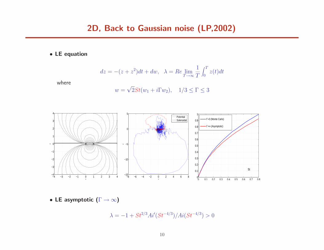
2D, Back to Gaussian noise (LP,2002)

• LE equation

dz = −(z + z2)dt + dw, λ = Re limT→∞

1

T

∫ T

0z(t)dt

wherew =

√2St(w1 + iΓw2), 1/3 ≤ Γ ≤ 3

x

y

−4 −3 −2 −1 0 1 2 3 4−4

−3

−2

−1

0

1

2

3

4

−8 −6 −4 −2 0 2 4 6 8−15

−10

−5

0

5

x

y

PotentialSolenoidal

0 0.1 0.2 0.3 0.4 0.5 0.6 0.7 0.80

0.1

0.2

0.3

0.4

0.5

0.6

0.7

0.8

0.9

1

St

Γ=3 (Monte Carlo)

Γ=∞ (Asymptotic)

• LE asymptotic (Γ → ∞)

λ = −1 + St2/3Ai′(St−4/3)/Ai(St−4/3) > 0

10

2D, Gaussian noise (Mehlig, Wilkinson et al, 2005)

11

Dispersion in 2D Kramers(LP,2005, 2008)

• Absolute (left) and relative (right) dispersion for different Hurst exponents α

10−1

100

101

102

10−1

100

101

102

103

104

105

time

t

10−1

100

101

102

10−2

100

102

104

106

time

t3

• Smooth space covariance (α = 2)

Three regimes in relative dispersion:

Ballistic: t2 or t3 depending on initial conditions

Exponential: exp (Λt) , Λτ(Λτ + 1)(Λτ + 2) = St

Inertial: t

12

Dispersion in 2D Kramers, cont’d

• Kramers with linear drift

·r= Gr + v·v= −v/τ+

·w (t, r)

G is constant matrix

• Existence of inertial regime for absolute dispersion

Inertial regime exists if and only if:

1. Drift is solenoidal and elliptic

2. Eigenvalues of G + 1/τ have positive real parts

3. τ <(

(g12 + g21)2/4 − g11g22

)−1/2

• Dispersion anisotropy

Absolute dispersion ellipse is the same as that of the drift.

The shape of relative dispersion ellipse depends on both, drift and normal covarianceparameters in fluctuations

• Diffusivity in a gyre

D =8σ2

uτ

1 + 4Ω2τ 2

13

Concluding remarks

• 1D Kraichnan with infinitely small correlation radius seems to remain the onlyexactly solvable coalescence model (LP and VP, 2000)

• Coalescence is comprehensively studied for non-smooth multi dimensional Kraich-

nan (Gawedzki and Vergassola 2000, Le Jan and Raimond, 2005, Gabrielli andCecconi, 2008,...)

• No coalescence is proven in Kramers (inertial particles)

• Clustering, ordering, dispersion and much more are comprehensively studied for

inertial particles (Bec, Elperin, Falkovich, Horvai, LP, Wilkinson,..., 2001-2009 )

14