www.iap.uni-jena.de

Lens Design II

Lecture 2: Structural modifications

2017-10-23

Herbert Gross

Winter term 2017

2

Preliminary Schedule Lens Design II 2017

1 16.10. Aberrations and optimization Repetition

2 23.10. Structural modifications Zero operands, lens splitting, lens addition, lens removal, material selection

3 30.10. Aspheres Correction with aspheres, Forbes approach, optimal location of aspheres, several aspheres

4 06.11. Freeforms Freeform surfaces, general aspects, surface description, quality assessment, initial systems

5 13.11. Field flattening Astigmatism and field curvature, thick meniscus, plus-minus pairs, field lenses

6 20.11. Chromatical correction I Achromatization, axial versus transversal, glass selection rules, burried surfaces

7 27.11. Chromatical correction II Secondary spectrum, apochromatic correction, aplanatic achromates, spherochromatism

8 04.12. Special correction topics I Symmetry, wide field systems, stop position, vignetting

9 11.12. Special correction topics II Telecentricity, monocentric systems, anamorphotic lenses, Scheimpflug systems

10 18.12. Higher order aberrations High NA systems, broken achromates, induced aberrations

11 08.01. Further topics Sensitivity, scan systems, eyepieces

12 15.01. Mirror systems special aspects, double passes, catadioptric systems

13 22.01. Zoom systems Mechanical compensation, optical compensation

14 30.01. Diffractive elements Color correction, ray equivalent model, straylight, third order aberrations, manufacturing

15 05.02. Realization aspects Tolerancing, adjustment

1. Correction strategy

2. Structural changes

3. Zero operations

4. Material optimization

3

Contents

Effectiveness of correction

features on aberration types

Correction Effectiveness

Aberration

Primary Aberration 5th Chromatic

Spherical A

berr

ation

Com

a

Astigm

atism

Petz

val C

urv

atu

re

Dis

tort

ion

5th

Ord

er

Spherical

Axia

l C

olo

r

Late

ral C

olo

r

Secondary

Spectr

um

Sphero

chro

matism

Lens Bending (a) (c) e (f)

Power Splitting

Power Combination a c f i j (k)

Distances (e) k

Lens P

ara

mete

rs

Stop Position

Refractive Index (b) (d) (g) (h)

Dispersion (i) (j) (l)

Relative Partial Disp. Mate

rial

GRIN

Cemented Surface b d g h i j l

Aplanatic Surface

Aspherical Surface

Mirror

Specia

l S

urf

aces

Diffractive Surface

Symmetry Principle

Acti

on

Str

uc

Field Lens

Makes a good impact.

Makes a smaller impact.

Makes a negligible impact.

Zero influence.

Ref : H. Zügge

4

Strategy of Correction and Optimization

If the potential of the setup seems to by not improvable, enlarge the number of degrees of freedom by structural changes of the system

Possible options are:

• add a lens

split a lens by distribution of nearly equal ray bending

split a lens by decomposing it by a positive and negative part

split a lens by decomposing it with two different materials

add especially a field lens

break a cemented component

insert a burried surface

• make a surface aspherical

• make a surface free shaped

• insert a mirror

• replace a lens by a mirror

• implement a diffractive surface

• remove a lens

• cement two lenses

• make an asphere spherical

5

Strategy of Correction and Optimization

Usefull options for accelerating a stagnated optimization:

split a lens

increase refractive index of positive lenses

lower refractive index of negative lenses

make surface with large spherical surface contribution aspherical

break cemented components

use glasses with anomalous partial dispersion

‚kick‘, if the optimization is captured in a local minimum

In general:

it is preferred to preserve the achieved (good) result and perform small changes

to let the optimization run again, change the weightings

if the potential of the setup seems to by not improvable, enlarge the number of degrees of freedom

6

Number of Lenses

Approximate number of spots

over the field as a function of

the number of lenses

Linear for small number of lenses.

Depends on mono-/polychromatic

design and aspherics.

Diffraction limited systems

with different field size and

aperture

Number of spots

12000

10000

8000

6000

4000

2000

00 2 4 6 8

Number of

elements

monochromatic

aspherical

mono-

chromatic

poly-

chromatic

14

diameter of field

[mm]

00 0.2 0.4 0.6 0.8

numerical

aperture1

8

6

4

2

106

2 412

8

lenses

single plano

convex lens

two plano

convex lenses

dublet of two

optimal

bended lenses

achromat

dublet with marginal

corrected ray and

residual zone

splitted achromate

achromate with

additional meniscus

four lenses

Wrms = 5.21

Wrms = 1.91

Wrms = 0.91

Wrms = 0.221

Wrms = 0.168

Wrms = 0.026

Wrms = 0.0159

Wrms = 0.0001

Spherical Aberration Correction

Correction of spherical aberration by splitting

the ray bending

Optimal bending of lenses

Splitting of lenses

Smooth reducing of spherical aberration

or marginal correction

8

Principle of Symmetry

Perfect symmetrical system: magnification m = -1

Stop in centre of symmetry

Symmetrical contributions of wave aberrations are doubled (spherical)

Asymmetrical contributions of wave aberration vanishes W(-x) = -W(x)

Easy correction of:

coma, distortion, chromatical change of magnification

front part rear part

2

1

3

9

10

Even Aberrations in Symmetrical Systems

Aberrations with even symmetry are doubled

Spherical aberration, Astigmatism, field curvature, axial chromatical aberration

Ref: M. Seesselberg

spherical aberration in an symmetrical system

4 4 9 9W c Z c Z

4 4 9 92 2W c Z c Z

4 4 9 9W c Z c Z

doubled values

11

Odd Aberrations in Symmetrical Systems

Ref: M. Seesselberg

Aberrations with odd symmetry are vanishing

Coma, distortion, transverse chromatical aberration

coma in an symmetrical system

8 8 15 15W c Z c Z 8 8 15 15W c Z c Z

0W

vanishing values

Symmetrical Systems

skew sphericalaberration

Ideal symmetrical systems:

Vanishing coma, distortion, lateral color aberration

Remaining residual aberrations:

1. spherical aberration

2. astigmatism

3. field curvature

4. axial chromatical aberration

5. skew spherical aberration

12

Symmetry Principle

Triplet Double Gauss (6 elements)

Double Gauss (7 elements)Biogon

Ref : H. Zügge

Application of symmetry principle: photographic lenses

Especially field dominant aberrations can be corrected

Also approximate fulfillment

of symmetry condition helps

significantly:

quasi symmetry

Realization of quasi-

symmetric setups in nearly

all photographic systems

13

14

Sensitivity by large Incidence

Small incidence angle of a ray:

small impact of centering error

Large incidence angle of a ray:

- strong non-linearity range of sin(i)

- large impact of decenter on

ray angle

Ref: H. Sun

ideal

surface

location

real surface

location:

decentered

ideal ray

real raysurface

normal

ideal ray

real ray

surface

normal

a) small incidence:

small impact of decenter

b) large incidence:

large impact of decenter

i

i

Distribution of refractive power

good: small W

Symmetry content

good: large S

General trend :

Cost of small W and large S : - long systems

- many lenses

Advantage of wj, sj-diagram :

Identification of strange surfaces

System Structure

N

j

jwN

W1

21j

NN

jjj

jun

y

m

nnw

''1

'

N

j

jsN

S1

21

j

j

j

j

NNstop

jj

jn

u

n

u

unin

in

ms

'

'

''1

1

|wj|

5 10 15 20 25 30 350

0.1

0.2

0.3

0.4

0.5

0.6

0.7

5 10 15 20 25 30 350

0.1

0.2

0.3

0.4

0.5

0.6

0.7

0.8

0.9

|sj|

power : W = 0.273

symmetry : S = 0.191

j

j

15

Example:

optimizing W and S with one additional lens

Starting system:

Final design

System Structure

|wj| |s

j|

1 2 3 4 5 6 7 8 9 10 110

0.5

1

1.5

2

1 2 3 4 5 6 7 8 9 10 110

0.2

0.4

0.6

0.8

1

1 2

3 45

67

8 910 11

S = 0.147W = 0.912

|wj| |s

j|

1 2 3 4 5 6 7 8 9 10 110

0.5

1

1.5

2

1 2 3 4 5 6 7 8 9 10 110

0.2

0.4

0.6

0.8

1

1 2

3 45

67

8 910 11

S = 0.147W = 0.912

|wj| |s

j|

1 2 3 4 5 6 7 8 9 10 11 12 130

0.2

0.4

0.6

0.8

1

1 2 3 4 5 6 7 8 9 10 11 12 130

0.5

1

1.5

2

W = 0.586 S = 0.182

1 2

3 4

5 6 789 10 11

12 13

|wj| |s

j|

1 2 3 4 5 6 7 8 9 10 11 12 130

0.2

0.4

0.6

0.8

1

1 2 3 4 5 6 7 8 9 10 11 12 130

0.5

1

1.5

2

W = 0.586 S = 0.182

1 2

3 4

5 6 789 10 11

12 13

16

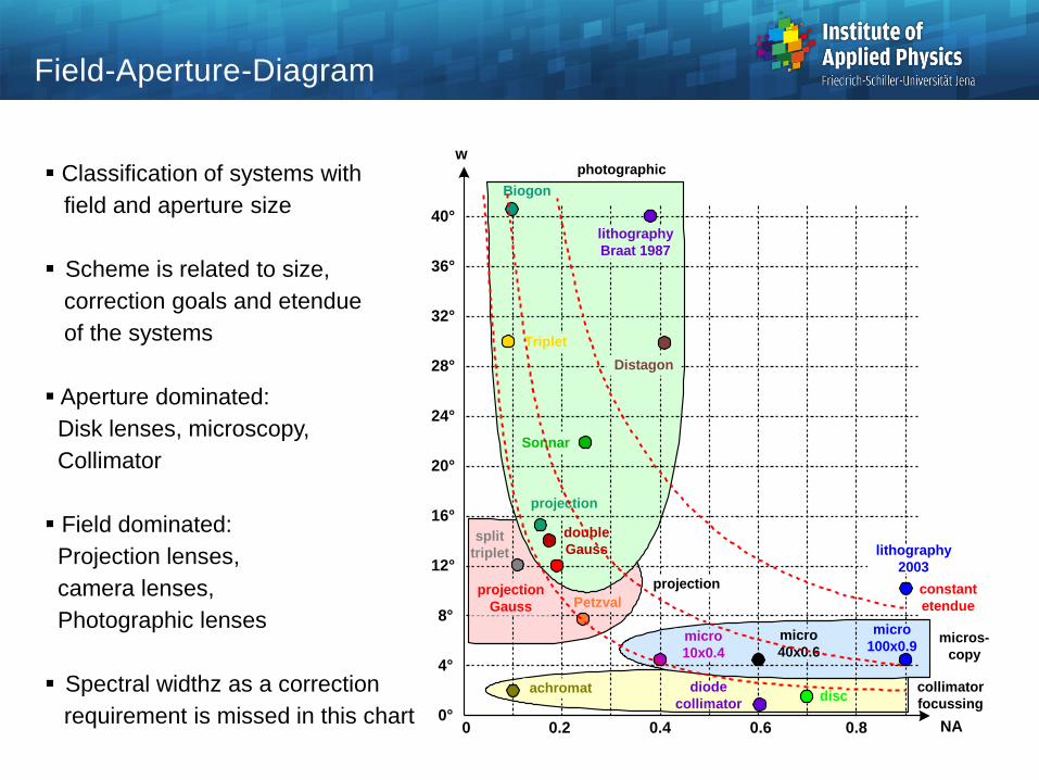
Field-Aperture-Diagram

0.20 0.4 0.6 0.80°

4°

8°

12°

16°

20°

24°

28°

32°

36°

NA

w

40°

micro

100x0.9

double

Gauss

achromat

Triplet

micro

40x0.6micro

10x0.4

Sonnar

Biogon

split

triplet

Distagon

disc

projection

Gauss

diode

collimator

projection

Petzval

micros-

copy

collimator

focussing

photographic

projection constant

etendue

lithography

Braat 1987

lithography

2003

Classification of systems with

field and aperture size

Scheme is related to size,

correction goals and etendue

of the systems

Aperture dominated:

Disk lenses, microscopy,

Collimator

Field dominated:

Projection lenses,

camera lenses,

Photographic lenses

Spectral widthz as a correction

requirement is missed in this chart

Variable focal length

f = 15 ...200 mm

Invariant:

object size y = 10 mm

numerical aperture NA = 0.1

Type of system changes:

- dominant spherical for large f

- dominant field for small f

Data:

18

Symmetrical Dublet

f = 200 mm

f = 100 mm

f = 50 mm

f = 20 mm

f = 15 mm

No

focal length [mm]

Length [mm]

spherical c9

field curvature c4

astigma-tism c5

1 200 808 3.37 -2.01 -2.27

2 100 408 1.65 1.19 -4.50

3 50 206 1.74 3.45 -7.34

4 20 75 0.98 3.93 2.31

5 15 59 0.20 16.7 -5.33

19

Field vs Aperture Correction

Remote pupil system with decreasing field for one wavelength and 4 lenses

Aperture maximum value for overall diffraction limited correction

Large field angles: lenses bended towards pupil

Old achromate move towards usual achromate

2 3 4 5 6 7 8 9 100

5

10

15

20

25

30

35

40

45

50

w [°]

D [mm]

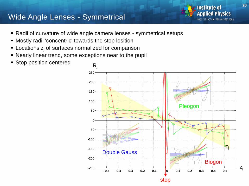
Radii of curvature of wide angle camera lenses - symmetrical setups

Mostly radii 'concentric' towards the stop losition

Locations zj of surfaces normalized for comparison

Nearly linear trend, some exceptions near to the pupil

Stop position centered

20

Wide Angle Lenses - Symmetrical

zj

Double Gauss

Pleogon

Rj

-0.5 -0.4 -0.3 -0.2 -0.1 0 0.1 0.2 0.3 0.4 0.5-250

-200

-150

-100

-50

0

50

100

150

200

250

Biogonzj

stop

Radii of curvature of wide angle camera lenses - asymmetrical setups

No clear trend

Locations zj of surfaces normalized for comparison

Stop position in the rear part

21

Wide Angle Lenses - Asymmetrical

Fisheye

Rj

Distagon

zj-1 -0.8 -0.6 -0.4 -0.2 0 0.2

-300

-200

-100

0

100

200

300Flektogon

stop

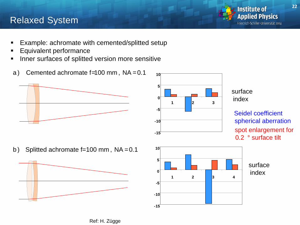
Relaxed System

Example: achromate with cemented/splitted setup

Equivalent performance

Inner surfaces of splitted version more sensitive

Ref: H. Zügge

a ) Cemented achromate f = 100 mm , NA = 0.1

b ) Splitted achromate f = 100 mm , NA = 0.1

-15

-10

-5

0

5

10

1 2 3

-15

-10

-5

0

5

10

1 2 3 4

Seidel coefficient

spherical aberration

spot enlargement for

0.2 ° surface tilt

surface

index

surface

index

22

Best Location for Correction Changes

The aberration contribution strongly depends on the heights of the marginal / chief ray

at a surface

Spherical aberration can be best corrected with a surface near to the pupil

Astigmatism and distortion can be best corrected with a surface near to the image

Field curvature does not depend on the surface location (see Petzval)

Coma correction depends on marginal and chief ray and thus is more complicated.

Usually a location near to the pupil is more helpful

23

Microscope Objective Lens

Seidel surface contributions

for 100x/0.90

No field flattening group

Lateral color in tube lens corrected

5 10

-0.5

0

0.5

-0.02

0

0.02

-4

-2

0

2

4

-5

0

5

-2

0

2

-0.02

0

0.02

-1

0

1

spherical

coma

astigmatism

curvature

distortion

axial

chromatic

lateral

chromatic

1

518

11

13

sum

24

Smooth changes

Lens bending

Distances

Structural changes:

Lens splitting

Power combinations

Structural and Smooth Changes for Correction

(a) (b) (c) (d) (e)

(a) (b)

Ref : H. Zügge

25

Operationen with zero changes in first approximation:

1. Bending a lens.

2. Flipping a lens into reverse orientation.

3. Flipping a lens group into reverse order.

4. Adding a field lens near the image plane.

5. Inserting a powerless thin or thick meniscus lens.

6. Introducing a thin aspheric plate.

7. Making a surface aspheric with negligible expansion constants.

8. Moving the stop position.

9. Inserting a buried surface for color correction, which does not affect the main

wavelength.

10. Removing a lens without refractive power.

11. Splitting an element into two lenses which are very close together but with the

same total refractive power.

12. Replacing a thick lens by two thin lenses, which have the same power as the two refracting

surfaces.

13. Cementing two lenses a very small distance apart and with nearly equal radii.

Zero-Operations

26

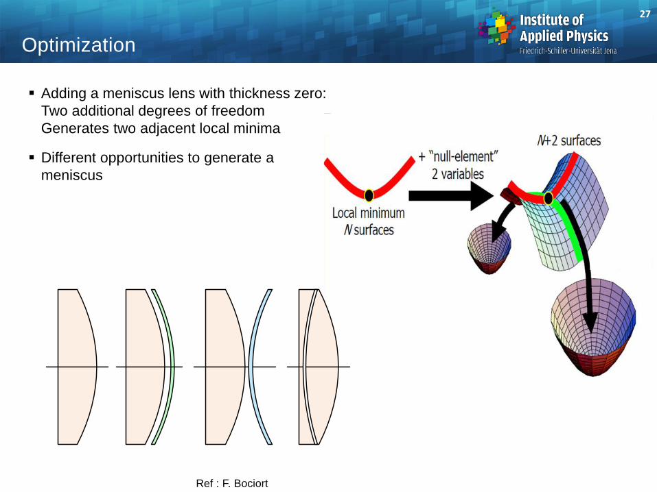
Adding a meniscus lens with thickness zero:

Two additional degrees of freedom

Generates two adjacent local minima

Different opportunities to generate a

meniscus

27

Optimization

Ref : F. Bociort

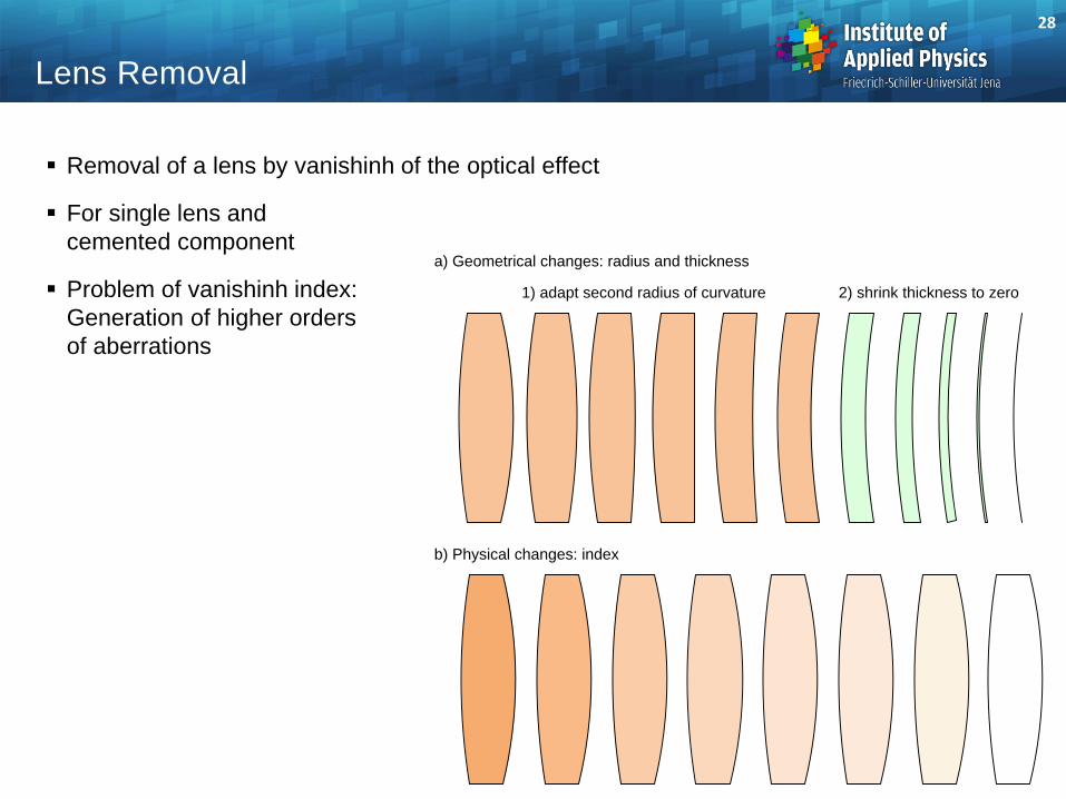
Removal of a lens by vanishinh of the optical effect

For single lens and

cemented component

Problem of vanishinh index:

Generation of higher orders

of aberrations

28

Lens Removal

1) adapt second radius of curvature 2) shrink thickness to zero

a) Geometrical changes: radius and thickness

b) Physical changes: index

Special problem in glass optimization:

finite area of definition with

discrete parameters n, n

Restricted permitted area as

one possible contraint

Model glass with continuous

values of n, n in a pre-phase

of glass selection,

freezing to the next adjacend

glass

Optimization: Discrete Materials

area of permitted

glasses in

optimization

n

1.4

1.5

1.6

1.7

1.8

1.9

2

100 90 80 70 60 50 40 30 20n

area of available

glasses

29

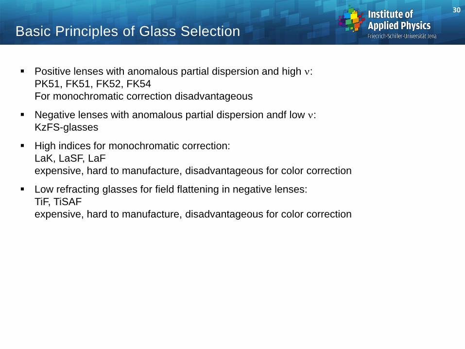
Positive lenses with anomalous partial dispersion and high n:

PK51, FK51, FK52, FK54

For monochromatic correction disadvantageous

Negative lenses with anomalous partial dispersion andf low n:

KzFS-glasses

High indices for monochromatic correction:

LaK, LaSF, LaF

expensive, hard to manufacture, disadvantageous for color correction

Low refracting glasses for field flattening in negative lenses:

TiF, TiSAF

expensive, hard to manufacture, disadvantageous for color correction

Basic Principles of Glass Selection

30

Principles of Glass Selection in Optimization

field flattening

Petzval curvature

color

correction

index n

dispersion n

positive

lens

negative

lens

-

-

+

-

+

+

availability

of glasses

Design rules for glass selection

Different design goals:

1. Color correction:

large dispersion

difference desired

2. Field flattening:

large index difference

desired

Ref : H. Zügge

31

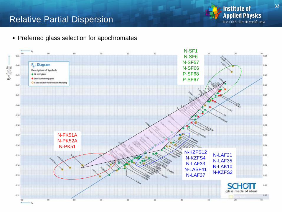
Preferred glass selection for apochromates

32

Relative Partial Dispersion

N-SF1

N-SF6

N-SF57

N-SF66

P-SF68

P-SF67

N-FK51A

N-PK52A

N-PK51

N-KZFS12

N-KZFS4

N-LAF33

N-LASF41

N-LAF37

N-LAF21

N-LAF35

N-LAK10

N-KZFS2

Cemented surface with perfect refrcative index match

No impact on monochromatic aberrations

Only influence on chromatical aberrations

Especially 3-fold cemented components are advantages

Can serve as a starting setup for chromatical correction with fulfilled monochromatic

correction

Special glass combinations with nearly perfect

parameters

d 1d 2 d 3

Nr Glas nd nd nd nd

1 SK16 1.62031 0.00001 60.28 22.32

F9 1.62030 37.96

2 SK5 1.58905 0.00003 61.23 20.26

LF2 1.58908 40.97

3 SSK2 1.62218 0.00004 53.13 17.06

F13 1.62222 36.07

4 SK7 1.60720 0.00002 59.47 10.23

BaF5 1.60718 49.24

Buried Surface

33