Nonlinearity 6 (1993) 549-568. Printed in the UK

Length scales in solutions of the NavierStokes equations

M V Bartuccellit$, C R Doeringf, J D Gibbont and S J A Malhamt T Depamnent of Mathematics, Imperial College, London SW7 282, UK 1 Department of Physics and Clsrkson Instihlte for Statistical Physics, Clarkson University, Potsdam NY 13699-5820, USA

Received 23 November 1992 Recommended by P Constantin

Abstract A set of ladder inequalities for the 2d and 3d forced NavierStokes equations on a periodic domain IO. LId is developed, leading to a nanrral definition of a set of length scales. We discuss what happens to these scales if intermittent flumations in the vorticity field occnr, and we consider how these scales compare to those derived from the attractor dimension and the number of determining modes. Our methods are based on estimates of ratios of norms which appear to play a natural role and which make many of lhe calculations comparatively easy. In 3d we cannot preclude length scales which are significantly shorter than the Kolmogorov length. In 2d OUT estimate for a length scale e tums out to be

(e/L)-* < cG(1 +logo)"*

where 9 is the Gmhof number. Tbis estimate. of e is shorter than that derived from the attractor dimension. The reason for this is discussed in detail.

PACS numbers: 4610

1. Introduction

The problem addressed in this paper concerns length scales arising in turbulence. To make both mathematical and physical sense, these scales should .arise naturally out of &e Navier-Stokes equations and should also make a connection with the length scales used, in conventional theories of turbulence. To be natural scales in a flow, they should also take into account, as much as possible, fluctuations in the vorticity away from spatial and temporal averages. Intermittent events may be rare, but may drive structures to substantially smaller scales than those associated with the long time periods when the Row remains close to these averages. Ideally, estimates for these scales will also be associated with results for the 3d Euler equations concerning the possible breakdown of regularity. In their paper on the breakdown of smooth solutions of the 3d incompressible Euler equations, Beale ef a1 [l] have shown that f,' llDu/,(r)dt (converted to f,' Ilollm(r)dr) conhols the possible breakdown of regularity in the 3d Euler equations. It has long been thought that a loss of regularity in the 3d Euler equations could have a major influence on the onset of Navier- Stokes turbulence (see the reviews by Majda [2,3]).

Whether singularities actually form in the 3d Euler equations is still an open question, but Beale, Kat0 and Majda's identification of 1,' llDuIl,(r)dr (or 1,' Ilollm(r)dr) as fhe

5 Resent address: D e m e n t of Mathematics, University of Suney, Guildford, UK

0951-7715/93/040549+20$07.50 @ 1993 IOP Publishing Ltd and LMS Publishing Ltd 549

550

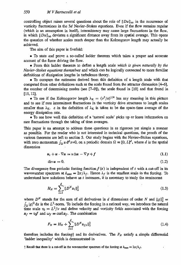
controlling object raises several questions about the role of llDullm in the occurrence of vorticity fluctuations in the 3d NavierStokes equations. Even if the flow remains regular (which is an assumption in itself), intermittency may cause large fluctuations in the flow, in which 11 Dull, deviates a significant distance away from its spatial average. This opens the question of whether scales much deeper than the Kolmogorov length may actually be achieved.

M V BiuhcceUi et al

The aim of this paper is fivefold

To state and prove a so-called ladder theorem which takes a proper and accurate account of the force driving the flow.

From this ladder theorem to define a length scale which is given naturally by the Nuvierstokes equations themselves and which can be Iogically connected to more familiar definitions of dissipation lengths in turbulence theory.

To compare the estimates derived from this definition of a length scale with that computed from other definitions such as the scale found from the attractor dimension [MI, the number of determining modes (see [7-9]), the scale found in [lo] and that found in [ l l , 121.

To see if the Kolmogorov length AK = ( U ~ / & ) ’ / ~ has any meaning in this picture and to see if rare intermittent fluctuations in the vorticity drive structures to length scales smaller than AK. E . in the definition of AK is taken to be the space-time average of the energy dissipation rate.

To see how well this definition of a ‘natural scale’ picks up or loses information on rare fluctuations through the taking of time averages. This paper is an attempt to address these questions in as rigorous yet simple a manner as possible. For the reader who is not interested in technical questions, the proofs of the various theorems are left to section 5. Our study begins with the NavierStokes equations, with zero momenhm Jn U ddx=O, on a periodic domain S l 5 [0, Lid, where d is the spatial dimension

ut + U . Vu = vAu - V p + f (1.1)

divu = 0. (1.2)

The divergence free periodic forcing functionf(x) is independent of t with a cut-off in its wavenumber specmm at k,, = k / A p Hence Ay id the smallest scale in the forcing. To understand how solutions behave as t increases, it is necessary to.study the seminorms

where DN stands for the sum of all derivatives in d dimensions of order N and llg11; = In 1gI2 dx is the L2-norm. To include the forcing in a rational way, we introduce the natural time scale TO = L z / u and define velocity and vorticity fields associated with the forcing .U/ = saf and my = curlq. The combination

(1.4)

therefore. includes the forcingt and its derivatives. The FN satisfy a.simple differential ‘ladder inequality’ which is demonstrated in

t Recall that there is a cut-off in the wavenumber spectrum of ,the forcing at bma. = 2n/Ay.

k n g t h scales in solutions of the Navier-Stokes equations 551

where

(1.6) *-2 - L-2 + *-2 , .

0 - f

and CN,$ are constants which depend only on N, s and d .

This theorem$ is a generalization of the ladder theorems in [IO]. Here we have a more precise statement of the effect of the forcing with the domain length and the cutoff scale in the forcing appearing in i o . To try to get Fo as the ‘bottom rung’ of either of our ladders, it is necessruy to take s = N . For either dimension d = 2 or d = 3, the negative definite terms are never quite strong enough to control the positive definite terms. Therefore, we are unable to prove the existence of an absorbing set in the appropriate function space solely with s = N . There are several different ways of trying to get around this, some of which are sharper than others, but all fail with s = N . Even for the 2d case one is forced, as in 3d, to take s = N - 1. In both the 2d and 3d cases therefore, F, is the ‘bottom mng’ of the ladder. In U, this quantity can be bounded above a priori (a result which is well known) thereby establishing regularity for the 2d case. section 4.2 deals with the 2d case further. Unfortunately, in 3d no a priori bound is known, in general, for the HI norm or any higher norms.

1.1. A natural definition of length scales

To see how theorem 1 naturally gives a set of length scales through the FN, we firstly look at the problem through a Fourier series expansion. Then we show that the ladder (1.5) gives a natural length scale associated with moments of the power spectrum.

(a) Fourier modes: Take a function g in 3d and write it in terms of its Fourier series

where the wavenumber K , as yet undetermined, divides between ‘low’ modes k i K and ‘high‘ modes k > K . After an application of the Schwarz inequality, this can be written as

for some s > 3/2. This can be written as

lkllm < C(K3/21k?llz +K3/2-sIIDsgllz) (1.9)

IIDru[lm < C(K3/zFi!s + K3/2-sF112 N )

Now we take g = D‘u and s fr = N and use (1.4) to get

(1.10)

t See section 5 for the pmof. § There is also an equivalent theorem (see [IO]) with v - ‘ ( U u l l ~ ~ instead of llDulloD and - v / Z instead of --Y

552

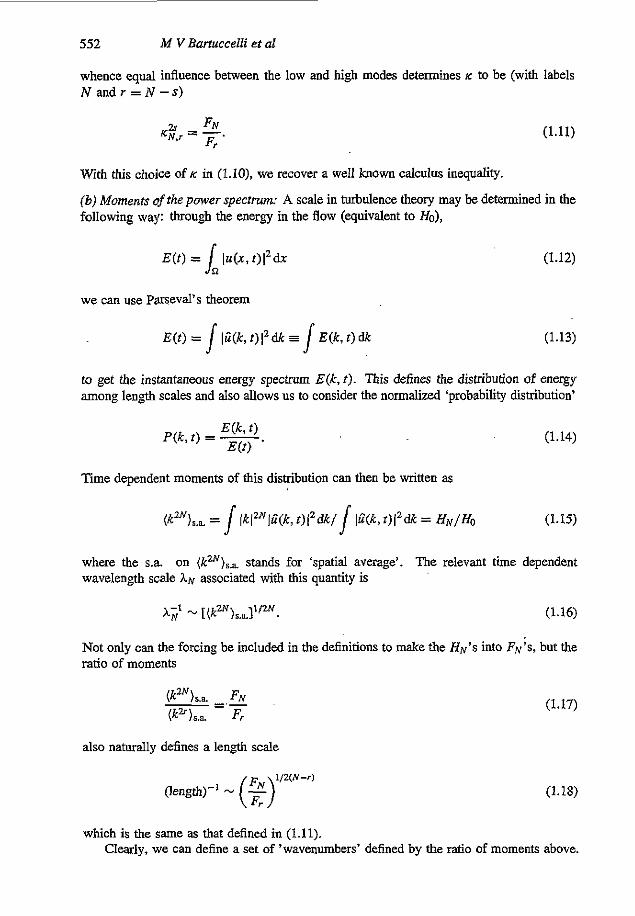
whence equal influence between the low and high modes determines K to be (with labels N and r = N - s )

M V Bartuccelli et a1

(1.11)

With this choice of K in (1.10), we recover a well known calculus inequaliw,

(b) Moments ofthe power spectrum: A scale in turbulence theory may be determined in the following way: through the energy in the flow (equivalent to Ho),

~ ( t ) = lu(x,t)12dx (1.12) s,

J J we can use ParseVal‘s theorem

E ( t ) = t)12& = E(k, t ) dk (1.13)

to get the instantaneous energy spectrum E(k, t). This defines the distribution of energy among length scales and also allows us to consider the normalized ‘probability distribution’

(1.14)

Time dependent moments of this distribution can then be written as

(kW)S.b = lkIzNIW, t ) l zdb l / lU (̂k, 0lz& = H N / H o (1.15)

where the s.a. on (kW)..& stands for ‘spatial average’. The relevant time dependent wavelength scale AN associated with this quantity is

- [ ( k Z N ) $ . & I ” . (1.16)

Not only can the forcing be included in the definitions to make the HN’S into FN’s, but the ratio of moments

also naturally defines a length scale

(1.17)

(1.18)

which is the same as that defined in (1.11). Clearly, we can define a set of ’wavenumbers’ defined by the ratio of moments above.

Length scales in solutions of the Navierdtokes equatiom 553

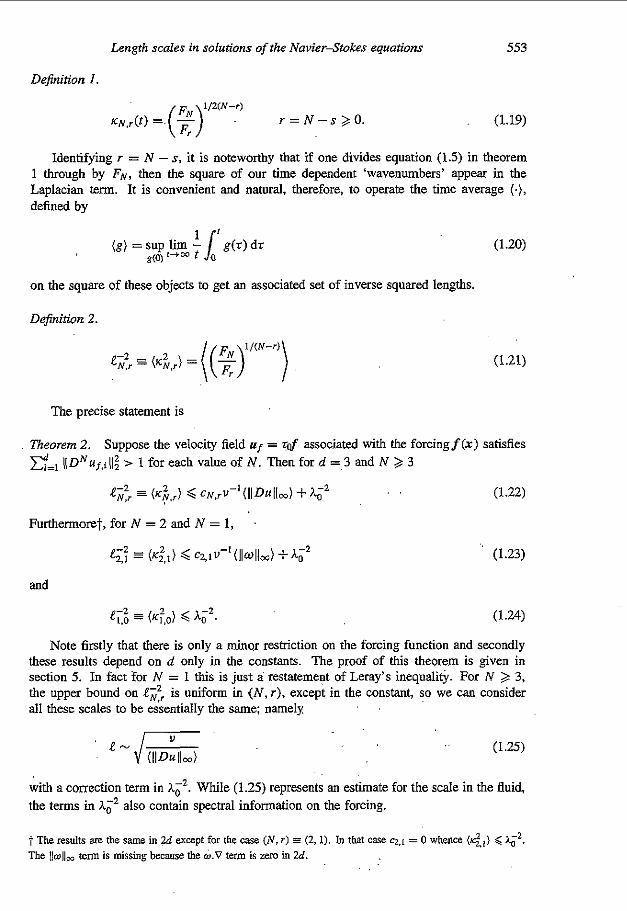
Definition 1.

(1.19)

Identifying r = N - s, it is noteworthy that if one divides equation (1.5) in theorem 1 through by FN, then the square of our time dependent ‘wavenumbers’ appear in the Laplacian term. It is convenient and natural, therefore, to operate the time average (.), defined by

1 ‘ *(a)’-- t a

(8) = sup lim - 1 g(r ) d t

on the square of these objects to get an associated set of inverse squared lengths.

Definition 2.

(1.20)

(1.21)

The precise statement is

Theorem 2. E:=, ((DNuf.iII; z 1 for each value of N. Then ford =,3 and N > 3

Suppose the velocity field uf = ?af associated with the forcingf(x) satisfies

e;:r = (K&) < CN,N’(IIDUII~) + hi2 . .

Furthermore?, for N = 2 and N = 1,

e;; = (K&} < C ~ , ~ U - ’ ( I I ~ I I ~ ) + h i 2

and

e-2 - 2 (,a = (K?,o) < h i .

Note firstly that there is only a minor restriction on the forcin these results devend on d only in the constants. The proof of I

(1.22)

(1.23)

function and secondly .s theorem is given in

section 5. In fact for N = 1 this is just a restatemept of Leray’s inequality. For N > 3, the upper bound on e;:, is uniform in ( N , r ) , except in the constant, so we can consider all these scales to be essentially the same: namely ’ ,

~ . (1.25) (IIDullm)

with a correction term in hiZ . While (1.25) represents an estimate for the scale in the fluid, the terms in A;’ also contain spectral information on the forcing.

t The results ae the same in 2d except for the a s e (N, r ) = (2, 1). In that case c1.1 = 0 whence (K&) 6 Ai’.

The llollm term is missing because the 0.0 term is zem in 2d.

554

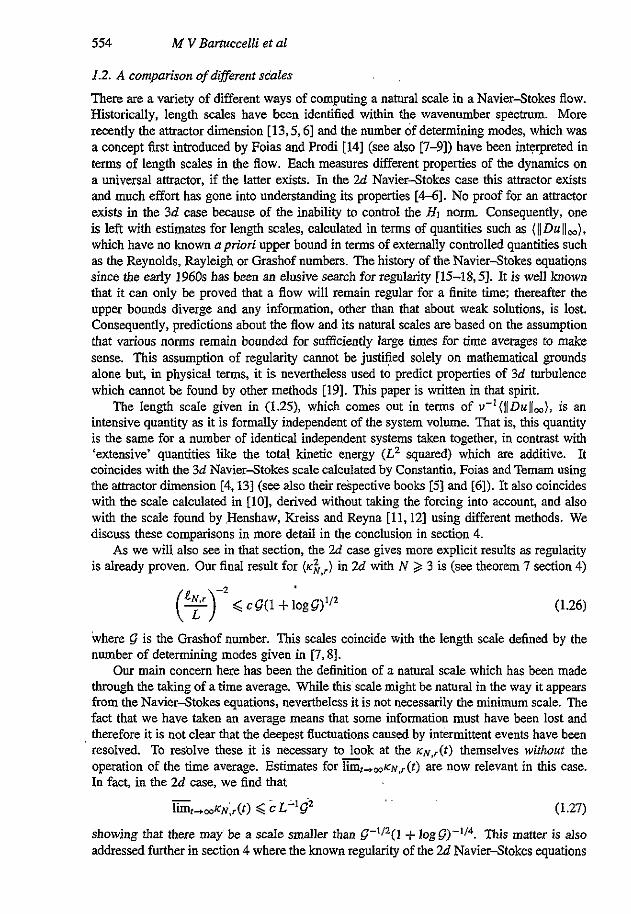
1.2. A comparison of different scales

There are a variety of different ways of computing a natural scale in a NavierStokes flow. Historically, length scales have been identified within the wavenumber spectrum. More recently the attractor dimension [13,5,6] and the number of determining modes, which was a concept first introduced by Foias and Prodi [14] (see also [7-9]) have been interpreted in terms of length scales in the flow. Each measures different properties of the dynamics on a universal attractor, if the latter exists. In the 2d NavierStokes case this attractor exists and much effort has gone into understanding its properties [ a ] . No proof for an attractor exists in the 3d case because of the inability to control the HI norm Consequently, one is left with estimates for length scales, calculated in terms of quantities such as ( I~DUII~), which have no known apriori upper bound in terms of externally controlled quantities such as the Reynolds, Rayleigh or Grashof numbers. The history of the NavierStokes equations since the early 1960s has been an elusive search for regularity 115-18,5]. It is well known that it can only be proved that a flow will remain regular for a finite time; thereafter the upper bounds diverge and any information, other than that about weak solutions, is lost. Consequently, predictions about the flow and its natural scales are based on the assumption that various norms remain bounded for sufficiently large times for time averages to make sense. This assumption of regularity cannot be justified solely on mathematical grounds alone but, in physical terms, it is nevertheless used to predict properties of 3d turbulence which cannot be found by other methods [19]. This paper is written in that spirit.

The length scale given in ( L E ) , which comes out in terms of u - ~ ( I ~ D u I ~ ~ ) , is an intensive quantity as it is formally independent of the system volume. That is, this quantity is the same for a number of identical independent systems taken together, in contrast with 'extensive' quantities like the total kinetic energy (L2 squared) which are additive. It coincides with the 3d NavierStokes scale calculated by Constantin, Foias and Temam using the attractor dimension [4,13] (see also their respective books 1.51 and [6]). It also coincides with the scale calculated in [IO], derived without taking the forcing into account, and also with the scale found by ,Hemhaw, Kreiss and Reyna [l l , 121 using different methods. We discuss these comparisons in more detail in the conclusion in section 4.

As we will also see in that section, the 2d case gives more explicit results as regularity is already proven. Our final result for (K;,,) in 2d with N 2 3 is (see theorem 7 section 4)

M V Bartuccelli et a1

(1.26)

where E is the Grashof number. This scales coincide with the length scale defined by the number of determining modes given in 17.81.

Our main concern here has been the definition of a natural scale which has been made through the taking of a time average. While this'scale might be natural in the way it appears from the NavierStokes equations, nevertheless it is not necessarily the minimum scale. The fact that we have taken an average means that some information must have been lost and therefore it is not clear that the deepest fluctuations caused by intermittent events have been resolved. To resolve these it is necessary to look at the K N , , ( ~ ) themselves without the operation of the time average. Estimates for Gr+m~~,r(t) are now relevant in this case. In fact, in the 2d case, we find that

( 1.27)

showing that there may' be a scale smaller than g-'lZ(l -+ log &?))-'I4. This matter is also addressed further in section 4 where the known regularity of the 2d NavierStokes equations

Length scales in solutions of the NavierSrOkes equations 555

makes matters easier to interpret. A further example used in that section is that of the complex Ginzburg - Landau equation where we illustrate the contrast between estimates for

For the moment, while this problem and a comparison with the other measures of dimension is left to section 4, it is instructive to see how our definition of a lene& scale compares with the way time averages are taken of moments to define a length scale in turbulence theory. In that approach, it is usual to consider the time averaged energy spectrum ( E & ) ) (which is the quantity which is supposed to decay algebraically in an inertial range). The relevant length scales are defined in terms of the average distribution of energy

( K ; , ~ ) and l imr+mKdt) .

(1.28)

This, of course, is not the same as time averaged instantaneous distribution of energy

( P ( k , . ) ) = ( dk’ E(k* . ) E (k’, .) ). (1.29)

A conventional definition of a len,& scale is calculated via (P) (k ) and so a ratio of time averages of the FN and F, would occur. In our natural (for NavierStokes) but slightly unconventional scale defined in (1.21) we have a time average of a ratio. Moments computed by taking the time average last are going to be more sensitive to rare, deep fluctuations in the vorticity down to short scales than those computed from the time-averaged energy specf”. This is because, all other things being equal, rare events contribute little to the average energy spectrum Moreover, when a significant fraction of energy is at high wavenumbers, the (relative) energy dissipation is necessarily higher, so these events will typicalIy be characterized by lower than normal total energy. They will then count little toward the time average of the energy spectrum. Dividing by the total energy before averaging therefore amplifies the role of the low energy but high wavenumber configurations in the distiibution, skewing the distribution towards high wavenumbers.

Consequently, despite our slightly unconventional definition, we assert that the scales defined by computing (F;,,) are natural to the NavierStokes equations and are likely to be more relevant to intermittent fluctuations than scales determined by the time-averaged energy spectrum (for example, the Kolmogorov length). As we have pointed out in the para-pphs above, however, whether this sensitivity goes far enough to pick up information on the smallest length scale is a different matter and is a point left for discussion in section 4.

2. Length scales during intermittency

As we have already discussed in section 1.2, predictions about the flow and its natural scales are based on the assumption that various norm$ remain bounded for sufficiently large times for time averages to make sense. We are particularly interested in the possibility that even if the flow remains regular (an assumption in itself), rare, large intermittent fluctuations or bursts in the vorticity field away from averages may nevertheless occur. If this is the case, a flow may remain close to its spatial average for large periods of time but, in short intervals, bursts in the vorticity field might cause the deep excursions mentioned above. The deeper they are, the rarer these events must be to avoid violating averages. This type of intermittency in the flow would likely be unpredictable. Because of the relatively long quiescent periods between these events, one has to think of how to compute a 1en-d scale

556 M VBQrtuccelli et a1

associated with the flow during these periods and then a second shorter scale associated with a burst if or when it occurs. It is in this situation that we would like to investigate the role of the Kolmogorov length XK. In particular, we would like to see whether AK is a natural scale, as is commonly assumed, or whether significantly shorter scales than this could possibly occur.

In the estimate from theorem 2, u-'([[Du[lm) is distinguished by the fact that it is expected to be an intensive quantity; that is, independent of system size. Formally, Constantin, Foias and Temam [MI estimate a Kolmogorov length from this quantity by defining an energy dissipation rate E, = u ( l l D ~ l l , ) ~ . Substitution of cm into theorem 2 gives

e;:r < c N , ~ A& + hi2 (2.1)

with

While this is mthennricaly a length scale, it is not the quantity which is normally understood to be the Kolmogorov len-6 based on an energy dissipation rate in (2.2) defined by E = u(llDull$) L-3. How are we to make a comparison between X K , ~ and XK? In so doing, one runs into an as yet insuperable problem. Using Gagliard+Nirenberg inequalifres to bound above an Lm norm by a W ( N , p ) norm (say), introduces the system volume into the problem thereby sacrificing the intuitive notion of an intensive length scale determined only by local properties of the flow. Let us begin by writing down haw many fixed (or bounded) scales exist against which we want to compare v-'(IIDullm).

A;' = LU2 + XK = ( ! J ~ / E ) ~ / ~ ; the Kolmogorov length. f i ~ = ( u ~ / E ~ ) ' / ~ ; the equivalent of the Kolmogorov length for the forcing.

the box length L and the smallest scale in the forcing Xf.

In their paper, Henshaw, Kreiss i d Reyna [12] use the approximation

(IID=llm) = L-3/2~11Du112) (2.3)

which makes

(2.4) ,p < -2 NJ \ N,r K,m + Fs cN.rAZ2 + hi2.

Physically, this approximation assumes that the dissipation in the flow is close to its spatial average, and that deviations away fiom thii state do not contribute to the time average. This assumption can only be true for those periods in the flow in between intermittent bursts in the vorticity field. Thus we expect the conventional Kolmogorov length to resolve the flow during the quiescent periods only when (2.3) holds. The phenomenon of spatial ,

intermittency, however, is associated with the energy dissipation being concentrated on a set of fractal dimension lower than the background space [ZO]. This leads to a fundamental violation of (2.3).

To see how far IIDull, is allowed to fluctuate away from IlDullz both in the time averaged sense and in the limsup sense, we prove

Length scales in solutions of the Navier-Stokes equations 557

Theorem 3. In 3d.

(IlDUllm) < ~ i ~ - ~ [ ( l l D ~ l l ~ ) + IlD~jll;l+ C Z W A O ~ + L-3’2(11D~11z) (2.5)

and

limr+mllDullm < CI U [hmt-,mllDull~ + llDuj11~1+ C Z V A ; ~ + L-3p~t~mllDu11z (2.6)

There is also the following corollary which turns (2.5) and (2.6) into inequalities in the

~.~ -3 ’ - -

vorticity:

Corollary 1.

( I I~ l lm) S c i ~ - ’ [ ( l l ~ I l ~ ) + ll@fIIil+ L-3’2(11~11z) + C Z U A ~ ~ (2.7)

and

limt,,liillm s c1u [limt+mIIoIIl + IIW& + L-~”&,~IIWIIZ + C P A . O ~ . (2.’8) -3 - -

Theorem 3, equation (2.5) demonstrates that

( K i , , ) < CAS$ < C A i 2 f i o 2 4- !-LK (IlDUlli) +IlDujlli . ~(2.9) (+I (z 1 The first of the two extra terms with the F4 coefficient, despite the disadvantage of being L dependent, is symbolic in pointing us to a mechanism of how large fluctuations to smaller scales than hK cannot be precluded. (IlDull$ is, in effect, the part which might become singularf in finite time should regularity fail. But even if it does not, the U-’ coefficient is significant in allowing this term to become large for high Reynolds numbers if the suprema in the time averages are reached. In consequence, we can see that AK is the natural scale only during those time periods between rare events when the vorticity in the fluid remains near its spatial average. These rare events will only occur if the fluid takes advantage of the slack allowed between the Lm and L2 norms in the theorem 3. Can we say exactly how short the length scales are down to which these rare events go? By these methods alone, the answer to this is ‘No’.

Theorem 3 is, in effect, only making a statement about what can happen as opposed to what will happen. Can we predict whether these vorticity bursts will actually occur? Nothing in our present methods indicate that they must happen nm do we have any handle on the possible sets of initial data that might cause them. Stepping into the realm of physics, it is not unreasonable to suppose that they are more likely to occur if the 3d Euler equations, exhibit finite time singularities. While this behaviour is not proven, it is generally believed that such singularities do occur (see the reviews by Majda [2,3]). A parallel can be drawn with the 2d/3d complex Ginzhurg Landau equation [21] where it’is known rigorously that its inviscid limit, the Nonlinear Schrodinger W S ) equation, exhibits finite time singularities.

Finally, as we have already compared llDullm with IlDullz, it is reasonable to ask whether any results of this type can be found for higher derivatives. Again, using the K N . ~ ,

the natural result is

t If the proof in theorem 3 is done slightly differently, we gef (tiJ) < ( ~ ~ , ~ ) ‘ ~ 2 ( l l D ~ l l ~ ) ’ ~ ~ . While (IIDull:) is bounded above, this calculation illustrates the well known closure problem in turbulence where high moments control low moments.

558

Theorem 4. For p 2 0, q = curl uf,

M V BartuccelIi et al

Apart from the constants, the right-hand side of equation (2.10) is independent of p .

3. F'roperties of K N , ~

In section 1 it was demonstrated that (K:,,) form a set of squared inverse lengths with the K N , ~ defined as

Here we take the argument further and show how they can be thought of as the natural mathematical objects through which some hown NavierStokes results can be derived in a simple and elegant way. In fact we will shortly show how they also arise naturally in a result of Beale et a1 [I] concerning the Euler equation. In the language of the HN of section 1, Leray's inequality tells us that ( H I ) is bounded above in any dimension. In the language of the KN, , , this translates to (K$ 4 1;' for both the 2d and 3d casest. The K N , ~ are ordered in an obvious way

K N ~ , , ( O 4 K N ~ . ~ ( ~ ) r < NI < Nz ~~ (3.2)

K N , ~ ~ ( ~ ) 4 K N . ~ @ ) ri < rz < N . (3.3)

Studying the possibility of control over, or of singularity formation in, this string is therefore equivalent to studying the problem of re-darity andor its breakdown.

Theorem 5. For the 3d NavierStokes equations with r c N - 1

(3.4) 2 2 (N 7 r ) h , r < CN.AIWI~~+ vi;') - U K N . A K N , , - K,+~,J.

and can be removed. Then a simple integration with respect to time gives Since K , + I . ~ 4 K N , ~ for r + 1 < N , the last set of terms in (3.4) are negative definite

This is, in effect, the equivalent of the Beale eta1 result [l] (which is implicit in their paper); namely, that ifregularity breaks down at t* < CO, then Jf IlDull,(s) ds must blow up at t*. No milder singularities are possible (see [2,3]). Since the last two'terms in theorem 5 can be removed in the inequality, the only part dependent on v and f is the "A;' term. For the Euler equations U = 0 and f = 0. This term vanishes from the theorem but the rest remains. Hence we have the equivalent result for the Euler equations. This reflects the joint results on the Euler and NavierStokes equations found by Constantin [22]. It is nice, however,

t We remind the reader that in 2d alone it~is also true that (K;,,) < "O', which is the generalization of (Hz) being bounded.

Length scales in solutions of the NavierSrokes equations 559

that the dynamic wavenumber itself k the quantity which is shown .to be controlled by the time integral of )I Dull,. The implications of this are discussed in section 4.

Jf. however, we want to convert estimates in llDullm into ones in Ilmll,. it is necessary to pay a price by introducing the system length L explicitly. The key to this is the inequality of Beale et al 111 which shows how IIDull, is controlled by 11011, on the domain CO, lI3:

IIDuIIw < C [ l fcIlmIIm(l +IOg+HdI IIOIIz. (3.6)

This inequality can be modified for the periodic domain [O, LI3 into

Lemma 1.

IlDullm < CN.7 lbl lm f lOg(LKN.,)l + L-3’z110h (3.7)

for N 2 3 and 0 < r < N. The + sign on the logarithm is defined such that log+ a = loga for a 2 1 and log* a = 0 otherwise.

The main point is that the K N , ~ ( N 2 3) are the natural ‘mediators’t between llDullco and IImll,. Another consecpence of the Beale et a1 result in the form given in lemma 1 is if we want to estimate the K N , , explicitly as functions of time in terms of the time integral of 11011,. An integration of the result of theorem 5 and lemma 1 gives

KN,r(f) < C L-’ eXp g(t‘) eXp[f(t) - f ( f ) ] dt’ (3.8)

where

(3.9)

and

g(t) = VA;’ + L-3/211~112. (3.10)

The result for the Euler equations is recovered by putting f = 0 and U = 0. Here we have a solution of the differential inequality for both the Euler and the NavierStokes equations in terms of the K N , ~ , instead of the HN norms alone [l].

Finally, instead of considering how j,” llDull&(r)dr controls the scales, it is possible to see how upper bounds on the K N , ~ can become singular (we take the case f = 0). Using the Gagliardo Nirenberg inequality for N 2 3

IIDullm < CKN,OIIUIIZ 5/2 (3.11)

and using this in theorem 5, we integrate with respect to time (ignoring the uAiZ term which does not change the nature, of the result), we obtain

f

[K(N,0)(o)l-5/2 - [ K ( N , 0 ) ( t ) l - S / 2 5 C 1 IlullZ(s) ds (3.12) 0

t As an aside, this result, together with (3.7) and theorem 1, lead us to a curious result in which we am able Lo find an estimate in terms of (Ilollm), not for (t;,,) but for ( K N . , ) ~ . Specifically, in 36 and for N > 3, (KN.,)’ < c’Q[l+Iog(L2Q)l where Q =h~2+h~7+~u-‘ ( l lwl lm). Theexplicit systemsizedependenceresides only in the logarithm. However, (KN.,)’ is less than the length scale defined in definition 2.

560

which, from the NavierStokes equations, is itself bounded by

M V Bartuccelli et a1

Ilu[Iz(s)ds < ~ L - ~ v - ' ~ [ u [ l ~ ( 0 ) [ 1 - exp(-cLzvr)J. (3.13)

In combination with (3.12), this gives

K,v,o(t) ,< C[KN,O(O)-~/~ - G(t)]-"5. (3.14)

The solution has no singularities if

[ K ~ , o ( o ) ] - ~ / ~ > Cz-zU-' [ l U [ l z ( o ) . (3.15)

For N 2 3, this result can be converted into

K N , c ~ ( ~ ) < L-'[CN&]-"~ (3.16)

where the Reynolds number Re, defined in terms of the initial conditions is

(3.17)

This is equivalent to the well known result of Ladyzhenskaya [15]; in this case, regularity can be achieved for high Reynolds numbers at the price of having the initial data on the third derivative very small.

4. Conclusion

4.1. Levels ofscales in 3d

One of the main tools in thii paper in examining len,.th scales has been the construction of the dynamic 'wavenumbers' KN,&) which, for N 2 3, have the property (K;,~) 6 c ~ , ~ u - ' ( [ l D u ~ l ~ ) +A;'. How do these scales compare with those found via the ,attractor dimension, and the number of determining modes respectively? In 3d, they coincide with the v-'(IIDullm) result of Constantin, Foias and Temam [5,4] and Foias era1 171. As we have pointed out in section 1, they also coincide with those found in [ll, 121. The fact that we have taken a time average could mean that some information about rare events in the flow may has been lost. We can conclude therefore that length scales may exist on three different levels.

e The first is the Kolmogorov length which will be the prevalent scale AK when Du lies close to its spatial average: i.e. (IlDull,) L-3/z(1[Du1[2)., This scale will be sufficient to resolve the flow during those long intervals when it remains quiescent. Indeed, there must be long time intervals between large intermittent events so as not to violate averages.

e If an intermittent event occurs but the flow remains regular, then during this event, the minimum length scale could become considerably shorter than AK, although down to what level it may go we cannot say without a regularity proof (see section 2).

e Even smaller scales than these are possible during events which our time average ( K ; , ~ ) has averaged out, thereby missing some information. These are the smallest scales of all and are ones which, realistically, are given by the KN,, themselves without the operation

Length scales in solutions of the Navier-Stokes equations 561

i&-tm~~.r. As we of the time average. We can write this inverse scale as (length)-' have already found from theorem 5,

(N - T ) K N , ~ ( ~ ) < K N A O ) exp ( ~ ~ . ~ l P ~ I l d r ) + vi;') dt. (4. I) Lr .~

This result returns us to the Beale et al result [I] for the 3d Euler equations, where it is shown that 1,' IIDullm(~) dr controls singularity formation. We cannot go beyond this without a regularity proof if the main part of the estimate is to be independent of system volume. If, however, we are willing to sacrifice intensivity then it is possible to find a limsup estimate directly for K N , ~ in terms of the HI norm.

Theorem 6. In d dimensions and for N z (414 - d)

where Q = u - 2 L 4 - d r im,-+,F1.

Since the KN,O are ordered such that KN>,o 6 KN~,o for NI < Nz, we must take the minimum of the right-hand side of the estimate in theorem 6, namely Qh". For d = 3, an examination of this shows that it is similar to the upper bound on the length scale derived in equation (2.9) using'the time average. The Qz estimate, in effect, when all the factors of L are accounted for, gives L J - ~ ~ & ~ F ? : there we had u - ~ ( F : ) . Although we would expect the latter to be higher, this is the only disparity between the two. Neither of these, (2.9) or (4.2), can be sharp because of the price paid by introducing the system volume into the problem and, with present methods, they are indeterminate. This inability to get a system size independent estimate is, we believe, due to the lack of a regularity proof. In the 2d case, when the NavierStokes equations are known to be regular, we are on surer ground in making comparisons between ( K ; , ~ ) and ( l i :+m~~,o)2 .

4.2. Length scales in the 2d Navier-Stokes case

While no explicit estimate for rapidly in the 2d case:

Theorem 7. In 2d

has been determined in 3d this can be achieved very

(L-'KN,?)* < c 8(1+ log8)"2. (4.3) (+IZ where G = v-ZL211f112 is the Grashof number.

In the proof in section 5 we have used the fact that (kz) ,< U ~ L - ~ G ~ . We have also ignored the A;' terms. The estimate in (4.3) coincides with the number of determining modes given in [7, SI but it is larger than the equivalent scale given by the attractor dimension 113,5,6,231

(4.4)

The left-hand sides of (4.3) and (4.4) are the number of degrees of freedom in a 2d system N = (L/l)2 which represents the number of 'eddies' of typical size .Cz that can fit in the

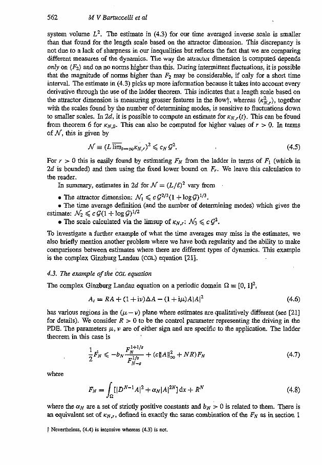
562

system volume Lz. The estimate in (4.3) for our time averaged inverse scale is smaller than that found for the length scale based on the attractor dimension. This discrepancy is not due to a lack of sharpness in our inequalities but reflects the fact that we are comparing different measures of the dynamics. The way the attractor dimension is computed depends onZy on ( F z ) and on no norms higher than this. During intermittent fluctuations, it is possible that the magnitode of norms higher than Fz may be considerable, if only for a short time interval. The estimate in (4.3) picks up more information because it takes into account every derivative through the use of the ladder theorem. This indicates that a length scale based on the attractor dimension is measuring grosser features in the flow?, whereas (K;,,), together with the scales found by the number of determining modes, is sensitive to fluctuations down to smaller scales. In Zd, it is possible to compute an estimate for KN,,(~). This can be found from theorem 6 for K N , ~ . This can also be computed for higher values of r z 0. In terms of N, this is given by

M V Bartuccelli et al

(4.5)

For r z 0 this is easily found by estimating FN from the ladder in terms of Fl (which in 2d is bounded) and then using the fixed lower bound on F,. We leave this calculation to the reader.

- 2 - N ( L limz+mKN,r) < CN Gz.

In summary, estimates in 2d for N = (L/@ vary from

The attractor dimension: NI < The time average definition (and the number of determining modes) which gives the

The scale calculated via the limsup of K N , ~ : N3 < c 8'.

+logG)'/'.

estimate: Nz < ~ G ( 1 + l o g G ) ' / ~

To investigate a further example of what the time averages may miss in the estimates, we also briefly mention another problem where we have both regularity and the ability to make comparisons between estimates where there are different types of dynamics. This example is the complex Ginzburg Landau (CGL) equation [21].

4.3. The example of the CGL equation

The complex Ginzburg Landau equation on a periodic domain Q = [0, l]',

A, = RA+(l+iu)AA-(l+ip)AIA1' (4.6)

has various regions in the (p - U) plane where estimates are qualitatively different (see [ZI] for details). We consider R > 0 to be the control parameEr representing the driving in the PDE. The parameters p, U are of either sign and are specific to the application. The ladder theorem in this case is , .

where the ( Y N are a set of strictly positive constants and b N 7 0 is related to them. There is an equivalent set of KN.,. defined in exactly the same combination of the FN as in section 1

t Nevertheless, (4.4) is intensive whereas (4.3) is not.

Length scales in solutions of the Navier-Stokes equations 563 .

for the Navier-Stokes equations. We will not go through every point in the analysis’ here; instead we describe the steps. Firstly, we find an estimate for IIAll, in terms of [IDA[[, and IlAllz and then use the same procedure as in the prooft oftheorems 2, 3 and 4. Then we find that

(K,?,,,) < 0, d R 3 + R. (4.9)

The point to note about this equation is that it is valid over the whole (p , U) plane and the parameter dependence on p and U is only in the multiplicative constant. While it is possible to improve this estimate to R in the so-called ’weak‘ region ( [ P I , [ V I small) described in 1211, where all solutions are strapped down close to their averages, the estimate given in (4.9) is valid in the so-called ‘strong’ region where IpI, IuI are large. It is in this region where one is close to the finite time singularity in the NLS equation. Moreover, the discrepancy between Lm and L2 norms can be vast if both R and IuI are chosen to be large. This is reflected in the estimate

- limt+m[lAll~ < R + c RIu1+’. (4.10)

Altogether, therefore, we expect spatially and temporally local intermittent events which can possibly$ get larger in amplitude because the exponent on the right-hand side of (4.10) is increasing with [ V I . It is clear, however, that the scale computed via the time average in (4.9) is not completely sensitive .to the, increasing magnitude of these fluctuations (except in the constant c(p, U)). To pick up the ‘spikes’, one would have to use the other definition given above for the NavierStokes equations: namely, i&,wKN,r(t). A repetition of the calculation equivalent to theorem I gives

L 2 ( G t , w K ~ , 1 ) 2 < R + C N Rl”’+l. (4.11)

5. Theorem proofs

In previous sections we promised to provide the proofs of the various theorems stated in this paper.

Proof of theorem 1 . With the definition ,

we h o w from [lo] that the HN satisfy

(5.2) ~ H N 1 ‘ < - ~ H N + I +CHNIIDUII~ + H;’*IIDNf 112.

H;+q < Hi+&-, (5.3j

Then it can be demonstrated, on a periodic domain [24] for q < M, that

t In Parallel with the minor restridon on the forcing in theorem 2, here we need R > 1. For 0 < R < 1, Ihe mactor is the origin. $ We say ‘possibly’ bemuse, to date, no definitive numerical study of Ihe spiky region has been performed.

564

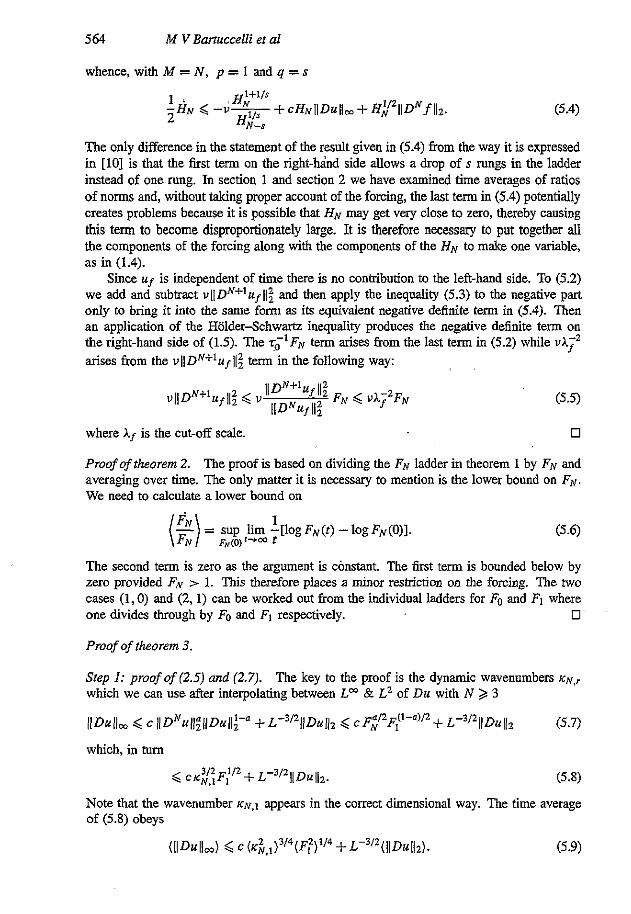
whence, with M = N , p = 1 and q = s

M V Bartuccelli et a1

(5.4)

The only difference in the statement of the result given in (5.4) kom the way it is expressed in [lo] is that the first term on the right-hand side allows a drop of s rungs in the ladder instead of one rung. In section 1 and section 2 we have examined time averages of ratios of norms and, without taking proper account of the forcing, the last term in (5.4) potentially creates problems because it is possible that HN may get very close to zero, thereby causing this term to become disproportionately large. It is therefore necessary to put together all the components of the forcing along with the components of the HN to make one variable, as in (1.4).

Since uf is independent of time there is no contribution to the left-hand side. To (5.2) we add and subtract ullDN+'uflli and then apply the inequality (5.3) to the negative part only to bring it into the same form as its equivalent negative definite term in (5.4). Then an application of the Holder-Schwartz inequality produces the negative definite term on the right-hand side of (1.5). The rilFN term arises from the last term in (5.2) while "AT* arises from the ~ l l D ~ + ~ u f l l $ term in the following way:

where A, is the cut-off scale. U

Proof of theorem 2. The proof is based on dividing the FN ladder in theorem 1 by FN and averaging over time. The only matter it is necessary to mention is the lower bound on FN. We need to calculate a lower bound on

The second term is zero as the argument is constant. The first term is bounded below by zero provided FN > 1. This therefore places a minor restriction on the forcing. The two cases (1.0) and (2, 1) can be worked out from the individual ladders for Fo and Fl where one divides through by Fo and FI respectively. 0~

Proof of theorem 3.

Step 1: proofof (2.5) and (2.7). The key to the proof is the dynamic wavenumbers K N , , which we can use after interpolating between Lm & Lz of Du with N 2 3

(IDulI, ,< c I(DNu(l~((Du(l~-' +L-3/21(DuI(~ ,< C F : / ~ F : ' - " ) ~ + L-3/z11Du((~ (5.7)

Note that the wavenumber KNJ appears in the correct dimensional way. The time average of (5.8) obeys

(IIDUIM G c ( K ~ , ~ ) ~ ~ ~ ( F ; ) ~ / ~ + L-~/~(IIDuII~). (5.9)

Length scales in solutions of the NavierStokes equatiom 565

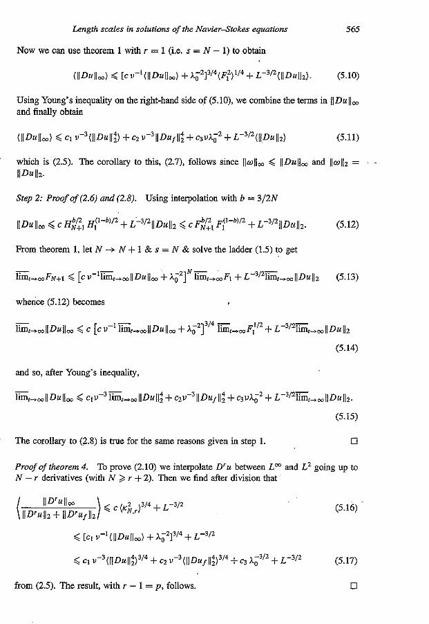
Now we can use theorem 1 with r = 1 (i.e. s = N - 1) to obtain

(IlDull,) < [cu-~(IIDuII~) +Ac213/4(F:)1/4+ L-3/z(11D~11z). (5.10)

Using Young's inequality on the right-hand side of(5.10), we combine the terms in 11 Dull, and finally obtain

(IlD~llm) 4 CI ~-~(IlDull:) + cz u-~IIDu~II: + c ~ u A , ~ +~L-3/2(11,D~11z) (5.11)

which is (2.5). The corollary to this, (2.7), follows since llullm < llDullm and llwllz = II~uIIz.

Step 2: Proof of (2.6) and (2.8). Using interpolation with b = 3f2N

[[Dullm < c Hi:, Hy") / z+ ,5-3/21]Du1]2 < c Fb12 N+1 F"-b)r- 1 + L-3/21jDullz.

From theorem 1, let N --f N + 1 & s = N & solve the ladder (1.5) to get

lim,,,FN+1 4 [ c u Iim,,,IIDuII, + A i Z ] lrmr+,4 + L-3/z~,+,IIDuIlz (5.13)

whence (5.12) becomes

~ r + , ~ ~ D u ~ ] w < c [cu-'i&.,llDuII, +,IOz]

(5.12)

- -1- N -

3/4 - ~~

lim,,,F~/2+ L-3/2~t,mIIDul12

(5.14)

and so, after Young's inequality,

-3 - - lim,.+,llDullw < CIU hm,+,llDull~ + CZU-~IIDU~II~ + C ~ V A ; ~ + L-3/2i&,,IIDu11~.

(5.15)

0

Proof of theorem 4. To prove (2.10) we interpolate D'u between Lm and L2 going up to N - r derivatives (with N

The corollary to (2.8) is true for the same reasons given in step 1.

r + 2). Then we find after division that

(5.16)

566

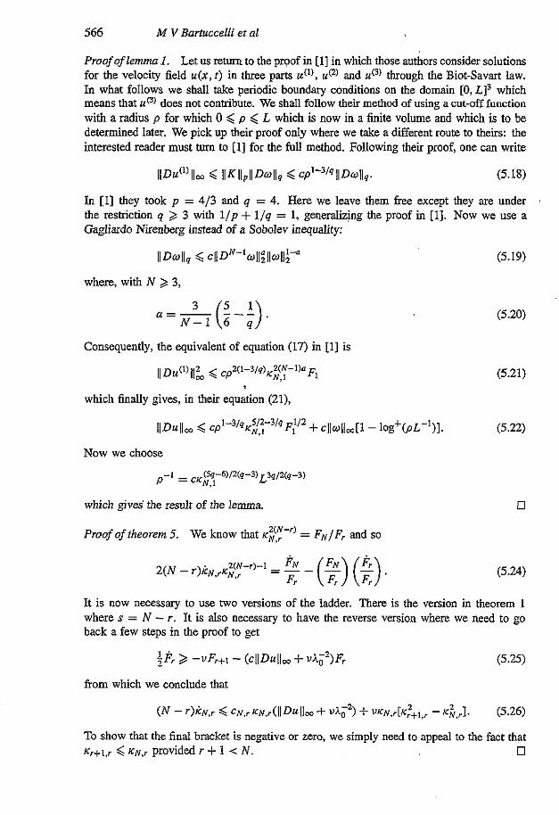
Proof of lemma I. Let us return to the proof in [l] in which those authors consider solutions for the velocity field U(& t) in three parts U('), U@) and U@) through the Biot-Savart law. In what follows we shall take periodic boundary conditions on the domain [O, LI3 which means that U@) does not contribute. We shall follow their method of using a cut-off function with a radius p for which 0 < p < L which is now in a finite volume and which is to be determined later. We pick up their proof only where we take a different route to theirs: the interested reader must turn to [l] for the full method. Following their proof, one can write

(5.18)

In [I] they took p = 413 and q = 4. Here we leave them free except they a e under the reshiction q > 3 with l / p + l / q = 1, generalizing the proof in 111. Now we use a Gagliardo Nirenberg instead of a Sobolev inequality:

I lDWl lq < cllDN-Loll;lloll:-' (5.19)

M V Bartuccelli er a1

IIDu(')Ilm < I l ~ l l p l l ~ ~ l l q < CP'-3/qIID~llq.

where, with N 2 3,

Consequently, the equivalent of equation (17) in [l] is

1 1 ~ ~ ( 1 ) l l 2 < 2(1--3/q) 'XN-Un m-. P KN.l '1

(5.20)

(5.21)

(5.22)

which gives' the result of the lemma U

Proof of theorem 5. We know that K ~ Y - ~ ) = FN/F, and so

(5.24)

It is now necessary to use two versions of the ladder. There is the version in theorem I where s = N - r. It is also necessary to have the reverse version where we need to go back a few steps in the proof to get

(5.25) 1 ' 5Fr 2 - v F r + ~ - (cllDullm + uA02)Fr

from which we conclude that

2 (N - T1kN.r < CN.r K N , r ( l l D U l l m + .A,") f U K N J [ K ? + I , ~ -KN,r]. (5.26)

To show that the final bracket is negative or zero, we simply need to appeal to the fact that 0 K , + , , ~ < K N , ~ provided r + 1 < N.

Length scales in solutions of the Navier-Stokes equations 567

Proof of theorem 6. We pursue a similar line to theorem 5 except that we take r = 0. The positive term from the Laplacian in (3.4), K N , O K ~ ~ = KN.OF,/FO. we obtain

NKN,o < - u K ~ , , , t (cdlD+, +2~a,-2) + V K N , O ( F I / F O ) . (5.27)

Because of the way FO is defined we know that it has a lower bound which can be used in the last term. This lower bound is FO r2]1 f 11;. From interpolation, we also know that

(5.28)

where we have used the fact that FO < L’FI. Using this in equation (5.27), the llDullm term in (5.28) is the strongest term competing with the -K:,, term and so we end up with

0

Proof of theorem’ 7. We use the logarithmic inequality of Brezis and Gallouet which estimates a 2d Lm norm in terms of HI but with a logarithmic correction which takes into account the HZ norm [25] (see also [23] for an easier and more informal proof). Taking into account our forcing term, 11 Dull, can be written

an absorbing ball for K ~ , O which gives the result.

(5.29)

Now we notice that F3/Fz = ~ 3 . 2 < K N , ~ for 2 < r < N with N t 3. Applications of first Cauchy’s and then Jensen’s inequality gives

(IlDUllw) < C (F2)”*[1 f 4 l0g(Lz(K~,z))1’/’. (5.30)

Now we can appeal to theorem 1 to &timate (IIDullw) by using the fact that (Fz) < W’L-~G’. In so doing we ignore the A;* terms. To do this we take the logarithm of both sides and use the fact that log( 1 f log Q ) < log Q for Q 2 1. This gives the result. 0

Acknowledgments

We acknowledge helpful discussions with Peter Constantin, Ciprian Foias, Darryl Holm, David Levermore, Andy Majda and Derek Moore. MVB would like to thank the UK SERC for a research assistantship and the CNR (Italy). CRD is supported on NSF Grants PHY- 8907755, PHY-8958506 and PHY 9214715. SJAV would also like to thank the UK SERC for a fees only studentship and the University of London for the Keddey Fletcher-Wan: studentship.

References

[l] Beale J T and Kat0 T and Majda A 1984 Remks on the breakdown of smooth solutions for the 3D Euler

[2] Majda A 1986 Vorticity and the mathemarical theory of incompressible fluid flow Commrm. Pure Appl.

[31 Majda A 199l.Vorticity, turbulence and acoustics in fluid flow SIAMRev. 33 349-88 141 Constanlin P, Foias C and Temam R 1985 Amctors representing Nhulent flows Memoirs of AMS

[51 Canstantin P and Foias C 1989 Navierdtokes Equations (Chicago, IL: Chicago University Press)

equations C o m x n . Math Phys. 94 61-6

Math 39 187-220

(Providence, RI: American Mathematical Society)

568 M V Bartuccelli et a1

Temam R 1988 Infinite dimensional dynamical systems in mechanics and physics Springer Applied

Foias C. Manley 0 P, Temam R and Treve Y M 1983 Asymptotic analysis of the NavierStokes equations

Constantin P, Foias C, Manley 0 P Ad Temam R 1985 Determining modes and fnctal dimension of

Manley 0 P and Treve Y M 1981 Minimum number of modes in approximate solutions to equations of

Bytuccelli M. Doering C and Gibbon J D 1991 Ladder theorems for the 20 and 3D NavierStokes equations

Henshaw W D, Kreiss H 0 and Reyna L G 1989 On smallest scale estimates for the incompressible

Henshaw W D, h i s s H 0 and Reyna L G 1991 Smallest scale estimates for the incompressible Navier-

Constantin P, Foias C and Temam R 1988 On the dimension of the attraCtors in two-dimensional turbulence

Foias C and Prodi G 1967 Sur le comporlement global des solutions non-stationnaires des equations de

Ladyzhenskaya 0 A 1969 The MnLemntical Theory of W".Y 1"compressible Plow 2nd edn (New York

Serrin J 1963 The initial value problem for the NavierStokes e+ations Nonlinear Probkm ed R E Langer

Temam R 1979 Nnvkr-Stokes Equntiom, Theory nnd Numerical Analysis (Amsterdam: North-Holland) Temam R 1983 The Navier-Stokes equations and non-linear functional analysis CBMS-NSFRegionol Cor$

Doering C R and Constantin P 1992 E n q y dissipation in shear driven Nrbulence PhyJ. Rev. ,?AI. 69

Prasad R K, Menevean C and Srienivasan K R 1988 Multif~actal nature of the dissipation field of passive

Bytuccelli M, Constantin P, Doering C R, Gibbon J D and GisselEilt M 1990 On the possibility of soft and

ConstanIin P 1986 Note on the loss of regularity for solutions of 3~ incompressible Euier and related

Doering C R and Gibbon J D 1991 Note on the Constantin-Foias-Temam amctor dimension for 2-

Bytuccelli M, Doering C R. Gibbon J D and Malham S J 1993 Lattice methods and the pmsure field for

Breds H and Callouet T 1980 Nonlinear Schrijdinger evolution equations Nonlinear AMly2is, Theory.

Mathematics Series "0168 (Berlin: Springer)

Physica D 9 157-88

turbulent flows 3. Fluid Mech. 150 427-440

hydrodynamics Phys. Len. 82A 88-90

on a finite periodic domain Nonlinenn'ty 4 53142

Navier-Stokes equations Theor. Compur. Fluid Dyn 1 65-95

Stokes equations Preprint

Physica D 30 284-96

Navier-Stokes en dimension 2 Rend. Sem Mat Podova 39 1-39

Gonion and Breach)

(Madison, WI: University of Wisconsin Press)

Series in Applied Mathemties (Philadelphia, PA SIAM)

1648-51

scaLvs in fully developed turbulent Rows Phys. Rev. Le& 61 74-7

hard turbulence in the complex Ginzburg-Landau equation Physica D 44 421-44

equations C o m ~ Math Phys. 104 311-29

dimensional turbulence Physica D 48 471-80

solutions of the Navier-Stokes equations Nonlinearity 6 79-91

Methodr nnd Applications 4 677481