Lectures on Contingency TablesElectronic edition

Steffen L. LauritzenAalborg University

October 2002

c© Copyright 1979, 1982, 1989, 2002 Steffen L. Lauritzen

Preface

The present set of lecture notes are prepared for the course “Statistik 2” at

the University of Copenhagen. It is a revised version of notes prepared in

connection with a series of lectures at the Swedish summerschool in Saro,

June 11–17, 1979.

The notes do by no means give a complete account of the theory of contin-

gency tables. They are based on the idea that the graph theoretic methods

in Darroch, Lauritzen and Speed (1978) can be used directly to develop this

theory and, hopefully, with some pedagogical advantages.

My thanks are due to the audience at the Swedish summerschool for

patiently listening to the first version of these lectures, to Joseph Verducci,

Stanford, who read the manuscript and suggested many improvements and

corrections, and to Ursula Hansen, who typed the manuscript.

Copenhagen, September 1979

Steffen L. Lauritzen

Preface to the second edition

The second edition is different from the first basically by the fact that a num-

ber of errors have been removed, certain simplifications have been achieved

and some recent results about collapsibility have been included.

I am indebted to Søren Asmussen, Copenhagen and Ole Barndorff-Nielsen,

Aarhus for most of these improvements.

Aalborg, August 1982

Steffen L. Lauritzen

1

Preface to the third edition

In the third edition more errors have been corrected and other minor changes

have been made. There has been some effort to bring the list of references

up to date.

Finally a section on other sampling schemes (Poisson models and sam-

pling with one fixed marginal) has been added. This section is based upon

notes by Inge Henningsen and I am grateful for her permission to include

this material.

Again Søren Asmussen and Søren Tolver Jensen have found errors and

made many detailed suggestions for improvements in the presentation. Helle

Andersen and Helle Westmark have helped transforming the typescript into

a typeset document. Søren L. Buhl has given me very helpful comments on

this manuscript. Thank you.

Aalborg, August 1989

Steffen L. Lauritzen

Preface to the electronic edition

The only essential changes from the third edition to this one is that some

figures and tables have been redrawn and some changes have been made to

the typesetting, to accomodate the electronic medium. Some references have

also been updated.

Klitgaarden, Skagen, October 2002

Steffen L. Lauritzen

2

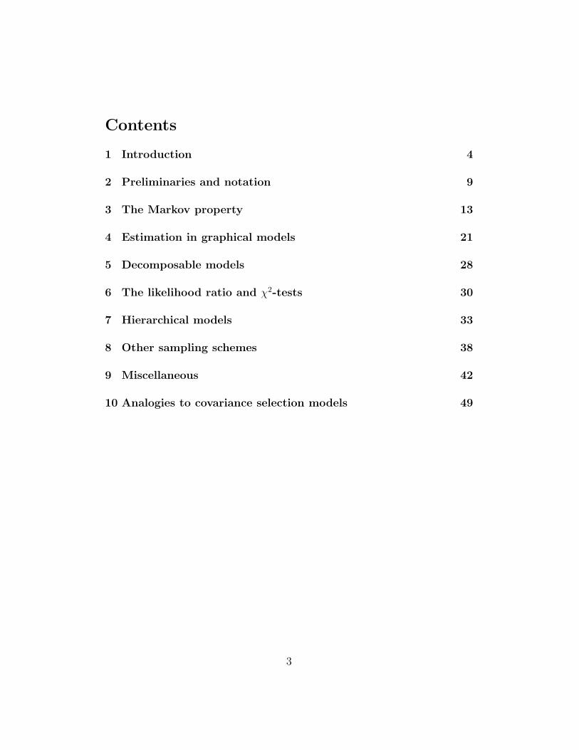
Contents

1 Introduction 4

2 Preliminaries and notation 9

3 The Markov property 13

4 Estimation in graphical models 21

5 Decomposable models 28

6 The likelihood ratio and χ2-tests 30

7 Hierarchical models 33

8 Other sampling schemes 38

9 Miscellaneous 42

10 Analogies to covariance selection models 49

3

1 Introduction

Before we proceed to develop the theory of multidimensional contingency

tables we shall briefly consider the basics of tables having dimension 2 or 3.

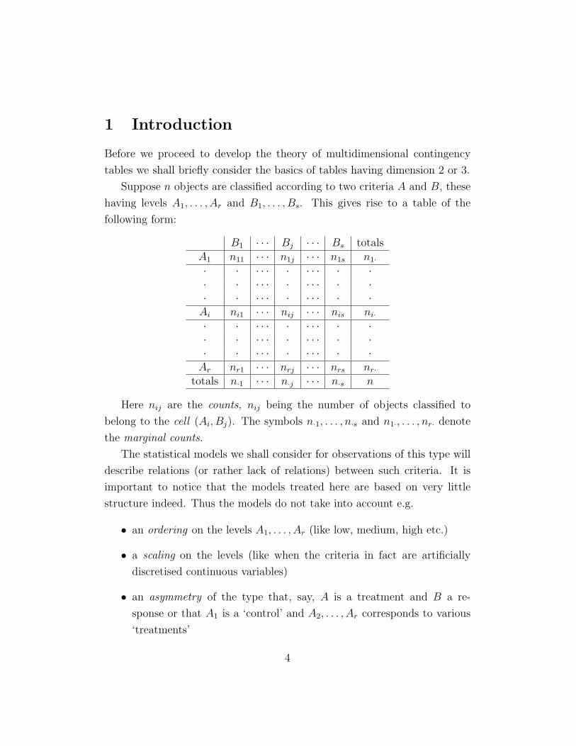
Suppose n objects are classified according to two criteria A and B, these

having levels A1, . . . , Ar and B1, . . . , Bs. This gives rise to a table of the

following form:

B1 · · · Bj · · · Bs totalsA1 n11 · · · n1j · · · n1s n1·· · · · · · · · · · ·· · · · · · · · · · ·· · · · · · · · · · ·Ai ni1 · · · nij · · · nis ni·· · · · · · · · · · ·· · · · · · · · · · ·· · · · · · · · · · ·Ar nr1 · · · nrj · · · nrs nr·

totals n·1 · · · n·j · · · n·s n

Here nij are the counts, nij being the number of objects classified to

belong to the cell (Ai, Bj). The symbols n·1, . . . , n·s and n1·, . . . , nr· denote

the marginal counts.

The statistical models we shall consider for observations of this type will

describe relations (or rather lack of relations) between such criteria. It is

important to notice that the models treated here are based on very little

structure indeed. Thus the models do not take into account e.g.

• an ordering on the levels A1, . . . , Ar (like low, medium, high etc.)

• a scaling on the levels (like when the criteria in fact are artificially

discretised continuous variables)

• an asymmetry of the type that, say, A is a treatment and B a re-

sponse or that A1 is a ‘control’ and A2, . . . , Ar corresponds to various

‘treatments’

4

• a theoretical knowledge about the probability structure. In e.g. genetics

where one can be interested in various linkage problems etc. there might

be a good a priori knowledge about the possible probability models.

It is a serious limitation on the usefulness of the models that structures

of the above kind disappear in the analysis. Nevertheless, any theory has

a starting point and the methods developed might be useful for a rough,

preliminary statistical analysis of many problems.

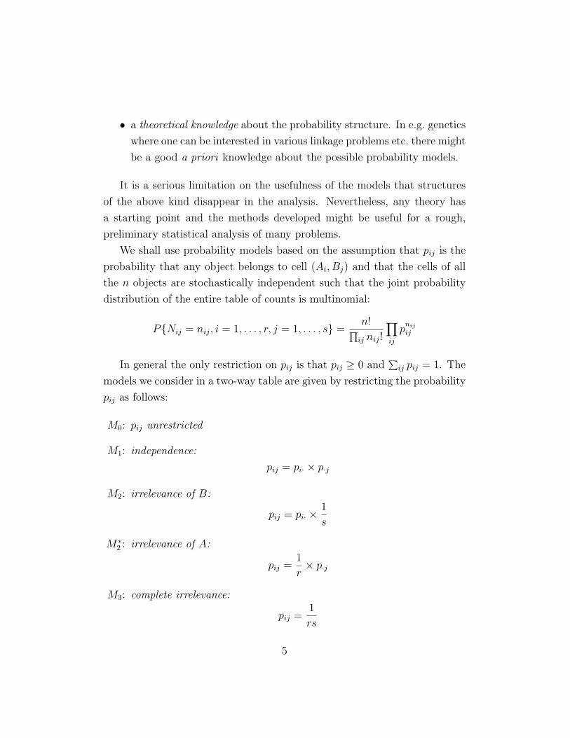
We shall use probability models based on the assumption that pij is the

probability that any object belongs to cell (Ai, Bj) and that the cells of all

the n objects are stochastically independent such that the joint probability

distribution of the entire table of counts is multinomial:

P{Nij = nij, i = 1, . . . , r, j = 1, . . . , s} =n!∏ij nij!

∏ij

pnij

ij

In general the only restriction on pij is that pij ≥ 0 and∑ij pij = 1. The

models we consider in a two-way table are given by restricting the probability

pij as follows:

M0: pij unrestricted

M1: independence:

pij = pi· × p·j

M2: irrelevance of B:

pij = pi· ×1

s

M∗2 : irrelevance of A:

pij =1

r× p·j

M3: complete irrelevance:

pij =1

rs

5

The models are clearly related as follows:

M0 ⊃ M1 ⊃M2

M∗2

⊃ M3

and the maximum likelihood estimate of the pij’s under assumptions of the

various models are given as:

M0:

pij =nijn

M1:

pij =ni·n× n·j

n

M2:

pij =ni·n× 1

s

M∗2 :

pij =1

r× n·j

n

M3:

pij =1

rs

The models can be tested by the likelihood ratio statistic which is given

as:

−2 logQ = 2∑ij

nij(log pij − log ˆpij),

where pij is the estimate of pij under the model assumed and ˆpij under that

to be tested. Of course the latter has to be a submodel of the former.

The likelihood ratio statistic can be approximated by the Pearson χ2-

statistic:

−2 logQ ≈ χ2 =∑ij

(npij − n ˆpij)2

n ˆpij

6

The exact distribution of any of these two statistics is in general in-

tractable and any practical inference has to be based on the asymptotic

distribution which can be shown to be χ2 with an appropriate number of

degrees of freedom. It is a delicate question to judge whether the asymptotic

results can be used in any practical situation and no clear results of practi-

cal use are known. A guideline is that n ˆpij should be large, which seldom

is the case for practical investigations with tables of high dimension. It is

sometimes possible to collapse tables so as to reduce the dimensionality. We

shall return to that later.

Three–way tables are treated mostly the same way. If nijk denote the

counts and pijk the cell probabilities, we can as before consider models as

e.g.

• independence between (A,B) and C:

pijk = pij· × p··k

• irrelevance of C

pijk = pij· ×1

t

where C ∼ C1, . . . , Ct

• complete independence

pijk = pi·· × p·j· × p··k

etc. etc.

But apart from these a new hypothesis naturally emerges stating that A and

C are conditionally independent given B:

pik|j = pi|j × pk|j

or equivalently

pijk =pij· × p·jk

p·j·.

7

If we look at the three–way table as a box, the condition B = Bj deter-

mines a slice, i.e. a two–dimensional table in A and C. The above hypothesis

corresponds to the assumption of independence in all these s two–way tables.

Under the assumption above, one can show that the maximum likelihood

estimate is given as

pijk =nij· × n·jkn·j· × n

.

Also in a three–way table the statistical inference can be based on the

analogous statistics

−2 logQ =∑ijk

nijk(log pijk − log ˆpijk) ≈∑ijk

(npijk − n ˆpijk)2

n ˆpijk.

Going from dimension 2 to 3, we saw that an essentially new kind of

model, that of conditional independence occurred. Generalizing to many

dimensions makes everything rather complex and such a generalization can

be made in different ways. We shall primarily be concerned with models

given by conditional independence, independence and irrelevance and try to

give tools that makes it possible to deal with all these such that the general

overview and insight does not disappear. The approach is based on the ideas

and results in Darroch, Lauritzen and Speed (1980).

A more usual way of developing the theory is to assume pijk > 0 and

make an expansion as

log pijk = α+ β1i + β2

j + β3k + γ12

ij + γ23jk + γ13

ik + δ123ijk

and then assume certain of these terms not to be present. The model of

conditional independence corresponds to assuming

δ123ijk ≡ 0 and γ13

ik ≡ 0.

Models of this type are denoted log–linear interaction models and the

terms in the expansion are denoted interactions. The method has the advan-

tage that it immediately generalizes to n dimensions but the disadvantage

8

that it becomes difficult to understand what the models in fact mean for the

problem that has to be analysed. Log-linear models and many other aspects

of the analysis of contingency tables are treated in detail in the classic book

by Bishop, Fienberg and Holland (1975).

One of the most difficult problems when the generalization has to be made

is to get a convenient notation. Therefore the next section will introduce a

new notation.

Secondly, since conditional independence becomes fundamental, we shall

briefly discuss the basic properties of this notion.

Finally, it shall turn out that the problem of dealing with many condi-

tional independencies is most easily taken care of by means of a little bit of

graph theory which also is contained in the following.

2 Preliminaries and notation

Let Γ be the set of classification criteria. Γ is supposed to be finite and |Γ| isthe number of elements in Γ. For each γ ∈ Γ there are levels Iγ which again

is a finite set. A cell in the table is a point i = (iγ)γ∈Γ where

i ∈ I = ×γ∈ΓIγ

We assume that n objects are classified and the set of counts

n(i) = the number of objects in cell i, i ∈ I

constitute the contingency table, such that

n =∑i∈I

n(i).

The number of criteria |Γ| is the dimension of the table. The marginal

tables are those given by only classifying the objects according to a subset

a ⊆ Γ of the criteria. We have the marginal cells ia = (iγ)γ∈a

ia ∈ Ia = ×γ∈aIγ

9

and the corresponding marginal counts

n(ia) = the number of objects in ia =∑

j:ja=ia

n(j).

As before we have the probabilities

p(i) = probability that an object belongs to cell i,

where p(i) ≥ 0 and∑i∈I p(i) = 1. And the joint distribution of the entire

table is multinomial:

P{N(i) = n(i), i ∈ I} =n!∏i n(i)!

∏i

p(i)n(i)

We are interested in marginal probabilities

p(ia) = probability that an object belongs to the marginal cell ia

=∑

j:ja=ia

p(j).

The notion of conditional independence is of great importance to us and

we say for three discrete–valued random variables X, Y and Z that X and

Y are conditionally independent given Z if

p(x, y | z) = p(x | z)p(y | z) whenever p(z) > 0

where p(x, y | z) is an imprecise but hopefully clear notation for

p(x, y | z) = P{X = x, Y = y | Z = z}.

If X and Y are conditionally independent given Z, we write

X ⊥⊥Y | Z.

Note that the following statements are true, where these all should be

read with the sentence following: ‘whenever all quantities are well–defined’:

CI0: X ⊥⊥Y | Z ⇔ p(x, y, z) = p(x, z)p(y, z)/p(z)

10

CI1: X ⊥⊥Y | Z ⇔ p(x | y, z) = p(x | z)

CI2: X ⊥⊥Y | Z ⇔ p(x, y | z) = p(x | z)p(y | z)

CI3: X ⊥⊥Y | Z ⇔ ∃f, g : p(x, y, z) = f(x, z)g(y, z)

CI4: X ⊥⊥Y | Z ⇔ p(x, y, z) = p(x | z)p(y, z)

The statements below give rules for deducing conditional independence

statements from others:

CI5: X ⊥⊥Y | Z ⇔ Y ⊥⊥X | Z

CI6: X ⊥⊥Y | Z ⇒ X ⊥⊥Y | (Z, f(Y ))

CI7: X ⊥⊥Y | Z ⇒ f(X,Z)⊥⊥Y | Z

CI8: [X ⊥⊥Y | Z and X ⊥⊥W | (Y, Z)] ⇒ X ⊥⊥ (Y,W ) | Z

The proof of all these assertions is an exercise in elementary probability

and omitted. In fact the rules CI5–CI8 can be used as a system of axioms for

probabilistic independence, such as pointed out by Dawid (1979, 1980). This

has also been further exploited to sketch a theory of irrelevance in connection

with the logic of reasoning cf. Pearl (1988).

We shall in our contingency table be especially interested in the random

variables corresponding to marginals such that we let Xa(i) = ia for a ⊆ Γ

and Xγ(i) = iγ for γ ∈ Γ. Instead of writing

Xa⊥⊥Xb | Xc

we shall simply write

a⊥⊥ b | c.

Only conditionally independencies of this type shall be dealt with.

We shall use the notion of a (simple, undirected) graph, i.e. a pair (V,E)

where V is a finite set, the vertex set, and E is a subset of the set of all

unordered pairs of V , the edge set. We display such a graph as e.g.

11

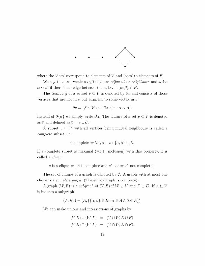
s s s s���

@@

@

@@

@

��

�s

ss

where the ‘dots’ correspond to elements of V and ‘bars’ to elements of E.

We say that two vertices α, β ∈ V are adjacent or neighbours and write

α ∼ β, if there is an edge between them, i.e. if {α, β} ∈ E.

The boundary of a subset v ⊆ V is denoted by ∂v and consists of those

vertices that are not in v but adjacent to some vertex in v:

∂v = {β ∈ V \ v | ∃α ∈ v : α ∼ β}.

Instead of ∂{α} we simply write ∂α. The closure of a set v ⊆ V is denoted

as v and defined as v = v ∪ ∂v.A subset v ⊆ V with all vertices being mutual neighbours is called a

complete subset, i.e.

v complete ⇔ ∀α, β ∈ v : {α, β} ∈ E.

If a complete subset is maximal (w.r.t. inclusion) with this property, it is

called a clique:

c is a clique ⇔ [ c is complete and c∗ ⊃ c⇒ c∗ not complete ].

The set of cliques of a graph is denoted by C. A graph with at most one

clique is a complete graph. (The empty graph is complete).

A graph (W,F ) is a subgraph of (V,E) if W ⊆ V and F ⊆ E. If A ⊆ V

it induces a subgraph

(A,EA) = (A, {{α, β} ∈ E : α ∈ A ∧ β ∈ A}).

We can make unions and intersections of graphs by

(V,E) ∪ (W,F ) = (V ∪W,E ∪ F )

(V,E) ∩ (W,F ) = (V ∩W,E ∩ F ).

12

If (V ∩W,E ∩ F ) is a complete graph we say that the above union is direct

and write

(V ∪W,E ∪ F ) = (V,E) ∪ (W,F ).

We then say that we have a decomposition of (V ∪W,E ∪ F ).

A path of length n in the graph (V,E) is a string of vertices α0, . . . , αn

such that αi−1 ∼ αi for i = 1, . . . , n. Note that a path can have length zero.

An n–cycle is a path of length n with α0 = αn.

We can define an equivalence relation on V as

α ∼p β ⇔ there is a path α0, . . . , αn with α0 = α, αn = β.

The subgraphs induced by the equivalence classes are the connected compo-

nents of (V,E). If there is only one equivalence class, we say that (V,E) is

connected.

Two subsets a, b of Γ are said to be separated by the subset c with a∩b ⊆ c

if all paths from a to b go via c, i.e. intersect c at some vertex. Note that if

(V ∪W,E ∪ F ) = (V,E) ∪ (W,F )

then V and W are separated by V ∩W in the graph (V ∪W,E ∪ F ). In

particular this holds for any decomposition. Thus two induced subgraphs

(a,Ea) and (b, Eb) form a decomposition of (Γ, E) if and only if

(i) a ∪ b = Γ

(ii) a ∩ b is complete

(iii) a ∩ b separates a \ b from b \ a.

We then say that a and b decompose (Γ, E).

3 The Markov property

The models shall be given by conditional independence restrictions of Markov

type: So let there be given a graph (V,E) with V ⊆ Γ.

13

Definition 1 A probability p is said to be Markov w.r.t. (V,E) if

M1: p(i) > 0 for all i ∈ I

M2: p(i) = p(iV )∏γ /∈V |Iγ|−1

M3: If α, β ∈ Γ, α 6∼ β then α⊥⊥β | Γ \ {α, β}.

A probability is extended Markov if p(i) = limn→∞ p(n)(i) where p(n) are all

Markov.

Note that M2 and M3 also hold for extended Markov probabilities whereas

M1 might be violated.

M2 corresponds to irrelevance of the criteria in Γ \ V . This implies that

these criteria can be ignored for statistical purposes and that the analysis

can be performed in the marginal table corresponding to V . It is thus no

severe restriction to assume V = Γ which is henceforth done.

A famous result due to many authors: Hammersley, Clifford, Spitzer,

Averintsev, Grimmett and others, asserts the equivalence between the Markov

property and the existence of an expansion of the logarithm of the probability

of a special structure. We shall let the functions for a ⊆ Γ, b ⊆ Γ

φa(i), Vb(i)

denote functions that depend on i through ia respectively ib only. Thus φ∅, V∅

are simply constants etc.

The theorem mentioned was once considered hard but now a simple proof

is available which is based on the following lemma.

Lemma 1 (Mobius Inversion) Let V and Φ be functions defined on the

set of all subsets of a finite set Γ. Then the following two statements are

equivalent:

(1) ∀a ⊆ Γ : V (a) =∑b⊆a Φ(b)

14

(2) ∀a ⊆ Γ : Φ(a) =∑b⊆a(−1)|a\b|V (b)

Proof We show (2) ⇒ (1):

∑b⊆a

Φ(b) =∑b⊆a

∑c⊆b

(−1)|b\c|V (c)

=∑c⊆a

V (c)(∑c⊆b⊆a

(−1)|b\c|)

=∑c⊆a

V (c)(∑h⊆a\c

(−1)|h|).

The latter sum is equal to zero unless a \ c = ∅ i.e. c = a, because any finite,

non–empty set has the same number of subsets of even as of odd cardinality.

The proof of (1) ⇒ (2) is performed analogously. 2

We are then ready to formulate and prove the following

Theorem 1 A probability p is Markov w.r.t. (Γ, E) if and only if there are

functions φa, a ⊆ Γ such that φa ≡ 0 unless a is a complete subset of Γ and

such that

log p(i) =∑a⊆Γ

φa(i). (1)

Proof Suppose we have the representation (1). The condition M1 is then

clearly fulfilled. Suppose now that α and β are not adjacent. This implies

that no complete subset can contain both α and β. We can then write

log p(i) =∑a∈A1

φa(i) +∑a∈A2

φa(i)

= ψ1(i) + ψ2(i)

with A1 = {a ⊆ Γ | α 6∈ a ∧ β ∈ a} and A2 = {a ⊆ Γ | β 6∈ a} so that ψ1

does not depend on iα and ψ2 does not depend on iβ. Thus

p(i) = eψ1(i)eψ2(i)

15

which gives us a factorisation as in CI3. Thus

α⊥⊥β | Γ \ {α, β}

i.e. we have shown that p is Markov.

Assume now p to be Markov. Choose a fixed but arbitrary cell i∗ ∈ I.

Define

Va(i) = log p(ia, i∗ac),

where (ia, i∗ac) is the cell j with jγ = iγ for γ ∈ a and jγ = i∗γ for γ 6∈ a. Let

further

φa(i) =∑b⊆a

(−1)|a\b|Vb(i).

Clearly, φa(i) depends only on i through ia. By the Mobius inversion lemma

we have

log p(i) = VΓ(i) =∑a⊆Γ

φa(i)

such that we have proved the theorem if we can show that φa ≡ 0 whenever

a is not a complete subset of Γ. So let us assume that α, β ∈ a and α 6∼ β.

Let further c = a \ {α, β}.Then we can write

φa(i) =∑b⊆c

(−1)|c\b|[Vb(i)− Vb∪{α}(i)− Vb∪{β}(i) + Vb∪{α,β}(i)

].

By M3 and CI4 we have, if we let d = b ∪ {α, β}

Vb∪{α,β}(i)− Vb∪{α}(i) = logp(ib, iα, iβ, i

∗dc)

p(ib, iα, i∗β, i∗dc)

= logp(iα | ib, i∗dc)p(iβ, ib, i

∗dc)

p(iα | ib, i∗dc)p(i∗β, ib, i∗dc)

= logp(i∗α | ib, i∗dc)p(iβ, ib, i

∗dc)

p(i∗α | ib, i∗dc)p(i∗β, ib, i∗dc)

= logp(ib, i

∗α, iβ, i

∗dc)

p(ib, i∗α, i∗β, i

∗dc)

= Vb∪{β}(i)− Vb(i).

16

Thus all terms in the square brackets are zero and henceforth the sum is

zero. This completes the proof. 2

The functions φa(i) in the above theorem are called interactions. If a

has only one element, φa is called a main effect. Since we have assumned

Γ = V all main effects are included in our representation (1). If a has m

elements, we say that φa is the interaction of (m − 1)’st order among the

criteria in a. In terms of interactions, the above theorem says that in a

Markov model, interactions are permitted exactly among neighbours. Main

effects are permitted exactly for those criteria that are not irrelevant.

Note that the representation (1) is not at all unique without imposing

further restrictions on the functions φa, a ⊆ Γ. Restrictions could be of the

symmetric type

b ⊂ a⇒∑

j:jb=ib

φa(j) = 0 (2)

for all a 6= ∅ and ib ∈ Ib, or of the type given by a reference cell

∀a 6= ∅ : φa(i) = 0 if iγ = i∗γ for some γ ∈ a (3)

where i∗ ∈ I is fixed but arbitrary.

The interactions constructed in the proof of Theorem 1 are the unique

interactions satisfying (3). For a systematic discussion of interaction repre-

sentations the reader is referred to Darroch and Speed (1983).

On the other hand, if (2) or (3) do not have to be satisfied, we can

construct a Markov probability by choosing any system of functions φa, a 6= ∅with φa ≡ 0 if a is not complete, and then adjust φ∅ such that the probability

given by (1) is properly normalised.

Using the rules of conditional independence given in Section 1, one can

of course derive a number of other conditional independence relations. This

can, however, be done once and for all and this is what we shall do by the

following:

17

Proposition 1 For a probability p with p(i) > 0, the following statements

are equivalent:

(1) p is Markov

(2) a⊥⊥ b | c, whenever c separates a and b

(3) ∀a ⊆ Γ : a⊥⊥ ac | ∂a

(4) ∀α ∈ Γ : α⊥⊥αc | ∂α

Proof

(1) ⇒ (2) : Consider the subgraph induced by Γ \ c. That c separates a and

b means that the vertices in a \ c and b \ c lie in different connected

components of this graph. Let A denote the vertices in components

containing vertices from a\c. Then A, c and Γ\ (A∪c) are disjoint and

a subset d of Γ can only be complete if either d ⊆ A ∪ c or d ⊆ Γ \ A.

By the exponential representation in Theorem 1 we have

p(i) = exp∑d

φd(i) = exp

∑d⊆A∪c

φd(i) +∑

d⊆Γ\A,d6⊆cφd(i)

since φd ≡ 0 unless d ⊆ A ∪ c or d ⊆ Γ \ A. By CI3 we get that

(A ∪ c)⊥⊥ (Γ \ A) | c and using CI7 twice gives a⊥⊥ b | c.

(2) ⇒ (3) : ∂a separates a from ac.

(3) ⇒ (4) : (4) is a special case of (3) if we let a = {α}

(4) ⇒ (1) : This follows from CI6 and CI7 since

α⊥⊥αc | ∂α⇒ α⊥⊥αc | Γ \ {α, β} ⇒ α⊥⊥β | Γ \ {α, β}

because β ∈ αc and β 6∈ ∂α since α 6∼ β.

18

This completes the proof. 2

The property (M3) is known as the pairwise Markov property, (2) is the

global Markov property and (4) is the local Markov property. They are not

equivalent in general without the positivity assumption (M1).

The global Markov property is strongest possible in the sense that if c does

not separate a and b, there is a Markov probability p such that, according to

p, a and b are not conditionally independent given c. Such a p can easily be

constructed using the exponential representation.

Thus (2) enables the researcher to read off all conditional independencies

implied by the graph.

In the case where the graph is of the type

s s s q q q s s swe get from Proposition 1 that {k}⊥⊥{1, . . . , k − 2} | {k − 1} for 3 ≤ k ≤ n

which exactly is the usual Markov property on the line. In other words, the

Markov property on a graph is an extension of the usual one.

If we consider extended Markov probabilities we have

p is extended Markov ⇒ (M3) ∧ (2) ∧ (3) ∧ (4).

This can be seen by arguing that (2) is satisfied, which we shall now do: Let

a, b, c be disjoint and assume that c separates a from b and that Γ = a∪ b∪ c.This can be done without loss of generality as in the proof of (1) ⇒ (2) in

Proposition 1. Since p is extended Markov we have p = lim pn and thus if

p(ic) > 0 we get from CI0 that

p(ia, ib, ic) = lim pn(ia, ib, ic)

= limpn(ia, ic)pn(ib, ic)

pn(ic)

19

=p(ia, ic)p(ib, ic)

p(ic)

whereby a⊥⊥ b | c as desired.

Thus the extended Markov probabilities have the same conditional inde-

pendence interpretations as the Markov ones, but no exponential represen-

tation as in Theorem 1. In other words, it is not meaningful in general to

discuss interactions for extended Markov probabilities.

When a and b form a decomposition of (Γ, E) the Markov property is

decomposed accordingly. More precisely we have, if we let 0/0=0

Proposition 2 Assume that a and b decompose (Γ, E). Then p(i) is (ex-

tended) Markov if and only if both p(ia) and p(ib) are (extended) Markov

w.r.t. (a,Ea) and (b, Eb) respectively and

p(i) =p(ia)p(ib)

p(ia∩b). (4)

Proof Suppose that p is Markov w.r.t. (Γ, E). Then (4) follows because

a ∩ b separates a \ b from b \ a. To show that p(ia) is Markov w.r.t. (a,Ea)

we show that if α 6∼ β and α, β ∈ a, then a \ {α, β} separates α from β in

(Γ, E). So let α, β be nonadjacent in vertices in a. Because a∩ b is complete,

at least one of them, say α, is in a \ b. If there were a path from α to β

avoiding a \ {α, β} it would go via b \ a contradicting that a \ b is separated

from b \ a by a ∩ b.The result for extended Markov probabilities follows by taking limits and

the converse is an immediate consequence of the exponential representation

(1). 2

For further results about Markov random fields see e.g. Kemeny, Snell

and Knapp (1976), Speed (1979) or Isham (1981).

20

4 Estimation in graphical models

We shall now consider the problem of finding the maximum likelihood es-

timate of the probability of any given cell under the assumption that this

probability belongs to the class of extended Markov probabilities with re-

spect to a given graph (Γ, E).

So let (Γ, E) be such a graph and let P be the set of Markov probabilities

w.r.t. (Γ, E). Let P denote the set of extended Markov probabilities. A

model of the type p ∈ P , is called a graphical model. Let C denote the class

of cliques of the graph (Γ, E). The likelihood function is proportional to

L(p) ∝∏i

p(i)n(i),

and we have to maximise this continuous function over the compact set of

extended Markov probabilities. Because we are considering P rather than

P , this maximum is always attained. We can further show that it is unique

and that it is given by a simple set of equations that roughly corresponds to

‘fitting the marginals’. Note that a probability p is an element of P if and

only if it can be expanded as

p(i) = exp∑c∈C

ψc(ic)

where C is the cliques of the graph (Γ, E). This is easily derived from the

exponential representation used in the main theorem of the previous section.

Note further that if p satisfies

L(p) = supp∈P

L(p)

then p(i) = 0 ⇒ n(i) = 0 i.e. n(i) > 0 ⇒ p(i) > 0. If this was not the case,

then L(p) would be equal to zero.

Let P∗be the set of p’s in P such that n(i) > 0 ⇒ p(i) > 0. Note that P∗

depends on the observed counts n(i), i ∈ I. Define for p ∈ P∗the operation

21

of ‘adjusting a marginal’ by

(Tcp)(i) = p(i)n(ic)/n

p(ic), where 0/0 = 0.

Note that Tcp is a probability and that (Tcp)(ic) = n(ic)/n. We have then

Lemma 2 The transformation Tc satisfies for all c ∈ C

i) Tc is continuous on P∗;

ii) Tc(P∗) ⊆ P∗

for all c ∈ C;

iii) L(Tcp) ≥ L(p) with equality if and only if p(ic) = n(ic)/n,∀ic ∈ Icwhich happens if and only if Tcp = p.

Proof Let ε > 0 and define πε(i) = (n(i) + ε)/(n + ε|I|). Then πε is a

strictly positive probability and for p ∈ P

(Tcp)(i) = limε→0

p(i)πε(ic)

p(ic).

It then follows from the exponential representation that

Tc(P) ⊆ P . (5)

If pm → p∗ with pm, p∗ ∈ P∗

we have

limm→∞

(Tcpm)(i) = limm→∞

pm(i)n(ic)/n

pm(ic)= (Tcp

∗)(i)

since this is evident if p∗(ic) > 0 and if p∗(ic) = 0, we must have n(ic) = 0

and the above relation is true as well. Thus i) is proved.

The continuity of Tc on P∗together with (5) implies now

Tc(P∗) ⊆ P .

But in fact we must have Tc(P∗) ⊆ P∗

since for p∗ ∈ P∗

(Tcp∗)(i) = p∗(i)

n(ic)/n

p∗(ic)

22

and if (Tcp∗)(i) = 0, p∗(i) = 0 or n(ic) = 0, both implying n(i) = 0 since

p∗ ∈ P∗and n(i) ≤ n(ic). Thus ii) is proved.

The last assertion of the lemma follows from

L(Tcp) = L(p)∏i∈I

(n(ic)/n

p(ic)

)n(i)

= L(p)∏ic∈Ic

(n(ic)/n

p(ic)

)n(ic)

and the latter factor is ≥ 1 and = 1 if and only if p(ic) = n(ic)/n by the

information inequality. 2

We are then ready to prove the main result.

Theorem 2 The maximum likelihood estimate p is the unique element of Psatisfying the system of equations

p(ic) = n(ic)/n, c ∈ C, ic ∈ Ic.

Proof The likelihood function is continuous on the compact set P such that

there is at least one p ∈ P such that

L(p) = supp∈P

L(p). (6)

But then p ∈ P∗as earlier noted and we get by Lemma 2 that

L(p) ≤ L(Tcp).

Further (6) gives the reverse inequality which implies L(p) = L(Tcp). and iii)

of Lemma 2 implies that p(ic) = n(ic)/n for all c ∈ C, ic ∈ Ic.Suppose conversely that p∗ ∈ P satisfies

p∗(ic) = n(ic)/n for all c ∈ C, ic ∈ Ic.

23

Then, for any p ∈ P , we have

logL(p) =∑i

n(i) log p(i)

=∑i

∑c

n(i)ψc(ic) =∑c

∑ic

n(ic)ψc(ic)

= n∑c

∑ic

p∗(ic)ψc(ic) = n∑

p∗(i) log p(i),

such that we by a continuity argument get that for all p ∈ P we have

L(p) =∏i

p(i)np∗(i).

But then we get by the information inequality

L(p∗) =∏i

p∗(i)np∗(i) ≥

∏i

p(i)np∗(i) = L(p).

By definition of p we have then equality and therefore p∗(i) = p(i) which

proves the uniqueness. 2

In general the maximum likelihood equations have to be solved iteratively.

The iterative procedure we shall give is known as the IPS-algorithm (Iterative

Proportional Scaling) and consists of successively fitting the marginals by

using the operations Tc, c ∈ C. More precisely, choose an ordering c1, . . . , ck

of the cliques and let

S = Tck · · ·Tc1 .

Choose further any p0 ∈ P∗

(e.g. p0(i) = |I|−1) and let

pm = Smp0.

Then we have

Theorem 3

p = limm→∞

pm.

24

Proof Let pmkbe a convergent subsequence, pmk

→ p∗. We have by the

continuity of L that

L(p∗) ≥ L(pmk) ≥ L(p0) > 0

such that p∗ ∈ P∗. Since also S is continuous on P∗

by Lemma 2 we have

L(Sp∗) = limk→∞

L(S(Smkp0))

≤ limk→∞

L(Smk+1p0) = limk→∞

L(pmk+1) = L(p∗).

Again by Lemma 2, L(Sp∗) ≥ L(p∗) such that we must have equality

L(Sp∗) = L(Tck−1· · ·Tc1p∗) = · · · = L(Tc1p

∗) = L(p∗).

Reading these from right to left and using iii) of Lemma 2 gives Tcp∗ = p∗

for all c ∈ C, i.e. p∗(ic) = n(ic)/n,∀c ∈ C,∀ic ∈ Ic. By Theorem 2 this

implies p∗ = p. Then we have shown that any convergent subsequence of pm

converges to p, which, by the compactness, implies pm → p. 2

Apart from using this algorithm it is sometimes possible to obtain the

maximum likelihood estimate in closed form. This is based on the fact that

sometimes some marginal probabilities can be estimated from a marginal

table, whereas it in general is necessary to estimate in the entire table and

afterwards calculate marginal probabilities. For example we have that, if c

is a clique

p(ic) = n(ic)/n

and this is obviously an explicit estimate of a marginal probability based on

a marginal table only. This trivially implies for a being any complete subset

of (Γ, E)

p(ia) = n(ia)/n.

But we can say much more about this. The important notion is that of a

decomposition. So let a, b be subsets of Γ such that the induced subgraphs

25

(a,Ea) and (b, Eb) define a decomposition of (Γ, E). This implies that a ∩ bseparates a \ b from b \ a and thus, by Proposition 1, we know that for all

p ∈ P we have

p(i) =p(ia)p(ib)

p(ia∩b)∀p ∈ P

where 0/0 = 0. But it also follows that the estimate decomposes in a similar

fashion, as we shall now see.

If we let pa(ia) denote the maximum likelihood estimate of p(ia) based on

the marginal counts n(ia) only and under the assumption that this marginal

probability is Markov (extended) w.r.t. (a,Ea) we have

Proposition 3 If a and b define a decomposition as above, then

p(i) =pa(ia)pb(ib)

n(ia∩b)/n.

Proof Since a and b are separated by a∩b we have for all cliques that either

c ⊆ a or c ⊆ b. Let Ca be the cliques of (a,Ea) and Cb the cliques of (b, Eb).

Then, clearly

C ⊆ Ca ∪ Cb.

The estimate pa is given by the fact that it is (extended) Markov w.r.t. (a,Ea)

and it satisfies

pa(ic) = n(ic)/n ∀c ∈ Ca,

and pb analogously. By Proposition 1 we can let

p∗(i) =pa(ia)pb(ib)

n(ia∩b)/n

and just show that p∗ satisfies the likelihood equations. But

p∗(ia) =∑

j:ja=ia

p∗(j) =pa(ia)pb(ia∩b)

n(ia∩b)/n= pa(ia)

since a ∩ b is complete. Thus for c ∈ Ca

p∗(ic) = pa(ic) = n(ic)/n

26

and similarly for c ∈ Cb, which proves the result. 2

Formulating this in a slightly different way, we get:

Corollary 1 If ∂(ac) is a complete subset then

pa(ia) = p(ia). (7)

Proof If we let b = ac ∪ ∂(ac) = ac then a and b define a decomposition

exactly when a ∩ b = ∂(ac) is a complete subset. Thus pa(ia) = p(ia). 2

The above corollary says in words that inference (or rather, estimation)

of relations among criteria in a can be performed in the marginal table when

∂(ac) is complete. This can be a useful tool in reducing the dimensionality

of any given problem.

The result in Corollary 1 can be considerably improved as pointed out to

me by Søren Asmussen. In fact we have

Proposition 4 If ∂b is complete for any connected component b of ac, then

pa(ia) = p(ia).

Proof Let ac = b1 ∪ · · · ∪ bk where bi are the connected components of ac.

Defining d = a∪b1∪· · ·∪bk−1 and e = bk∪∂bk, d and e define a decomposition

since

d ∩ e = (a ∪ b1 ∪ · · · ∪ bk−1) ∩ (bk ∪ ∂bk) = a ∩ ∂bk = ∂bk

which is complete by assumption. Thus

pd(id) = p(id).

By repeating the argument until all bi have been removed, we reach the

conclusion. 2

If a fulfills the condition of Proposition 4 we say that the graphical model

given by (Γ, E) is collapsible onto the variables in a.

27

A systematic investigation of this notion has been given by Asmussen and

Edwards (1983), where it is also shown that the condition in Proposition 4

is necessary for (7) to hold for any set of counts.

5 Decomposable models

In the previous section we discussed the notion of a decomposition and

showed that when a and b gave rise to a decomposition of (Γ, E), we could re-

duce the estimation problem to two marginal problems and a multiplication.

Sometimes we can now decompose further such that e.g. (a,Ea) decompose

into (a1, Ea1) and (a2, Ea2). If we can continue with this procedure such

that finally all the marginal problems ak are complete graphs, these marginal

models correspond to simple estimates, since we have

pak(iak

) = n(iak)/n

and the entire estimate for the probability is then obtained by a multiplica-

tion of all these relative frequencies and divisions with relative frequencies

corresponding to the intersections. In such cases we say that a model is

decomposable. More formally we define

Definition 2 The graph (Γ, E) is decomposable if either (Γ, E) is complete

or there exists a, b ⊆ Γ with |a| < |Γ| and |b| < Γ such that a and b decompose

(Γ, E) and such that (a,E1) and (b, Eb) are both decomposable.

An alternative to this recursive definition is to say that there exists an or-

dering c1, . . . , cn of the cliques of the graph such that for all i, ci and ∪j<icjdecompose the subgraph induced by ∪j≤icj.

Graphs having this property have been studied by graph-theorists for

many years and are known as triangulated graphs, rigid circuit graphs, chordal

graphs and other names as well. We shall state the following result without

proof but refer to e.g. Lauritzen, Speed and Vijayan (1984).

28

Proposition 5 A graph is decomposable if and only if it contains no cycles

of length ≥ 4 without a chord.

Here a cycle is a sequence of vertices α0, α1, . . . , αn with α0 = αn and αi ∼αi+1. Then n is the length. A chord is two vertices αi, αj such that αi ∼ αj

but j 6= i− 1, i+ 1 (modulo n).

Thus the smallest non-decomposable graph is the 4-cycle:

ssss

wehereas e.g. the graph

s���

@@

@

@@

@

��

�s

ss s1

2

3

4

5

is decomposable because the 4-cycle (2,3,4,1,2) has the chord (1,3).

As earlier mentioned, the maximum likelihood estimate can then be com-

puted by an explicit formula, multiplying together relative frequencies. We

shall here just mention that for a connected graph this has the form:

p(i) =1

n

∏d∈D

n(id)ν(d)

where ν(d), d ∈ D is an index defined on D, the set of all complete subsets

of the graph. This index is related to the number of connected components

of the graph when d is removed, see Lauritzen, Speed and Vijayan (1984).

If a graph is not connected, its components are independent and we get the

estimate by multiplying together the estimates from different components.

Decomposability can be exploited for efficient computation of estimates

but it can also be used as a basis for efficient computation of probabilities in

expert systems, see Lauritzen and Spiegelhalter (1988).

29

6 The likelihood ratio and χ2-tests

Consider now a subgraph (Γ0, E0) ⊆ (Γ, E) and let P = P(Γ,E) and P0 =

P(Γ0,E0). Clearly we have

P0 ⊆ P

such that we can ask for the likelihood ratio test for the hypothesis that

p ∈ P0 under the hypothesis that p ∈ P . In principle, given the estimation

results, it is no problem to compute the likelihood ratio test statistic as

−2 logQ = 2∑i

n(i) logp(i)

p0(i)

where p, p0 are the maximum likelihood estimates of p under P and P0 re-

spectively. This can be approximated by the Pearson χ2-statistic

−2 logQ ≈ χ2 =∑i

(np(i)− np0(i))2

np0(i).

Under the assumption that p ∈ P0, both the −2 logQ and χ2-statistics

have an asymptotic χ2-distribution with degrees of freedom equal to

dim(P)− dim(P0).

The dimensions can be obtained by the following rules

(i) If (Γ, E) is complete

dim(P(Γ,E)) =∏γ∈Γ

|Iγ| − 1.

(ii) If Γ = a ∪ b and E = Ea ∪ Eb then

dim(P(Γ,E)) = dim(P(a,Ea)) + dim(P(b,Eb))− dim(P(a∩b,Ea∩b)).

30

The correctness of these rules is a consequence of the following facts. First,

let for any c ⊆ Γ the symbol Lc denote the vector space of functions of i that

only depend on the c-marginal, i.e. on i through ic only. These obviously

satisfy

Lc ∩ Ld = Lc∩d

and

dim(Lc) =∏γ∈c|Iγ|.

Letting C denote the cliques of (Γ, E) we have for an arbitrary positive prob-

ability p that

p ∈ P(Γ,E) ⇔ log p ∈∑c∈C

Lc = HC

i.e. the probabilities in P(Γ,E) can be injectively parametrised by the set of

vectors θ ∈ HC satisfying ∑i

eθ(i) = 1.

The set P(Γ,E) is therefore a smooth surface of dimension dim(HC) − 1.

This reduces to (i) if C has only one element, i.e. if the graph is complete.

To prove the recursion formula we first note that

HC = HCa +HCb,

where Ca and Cb are the cliques of (a,Ea) and (b, Eb) respectively. It remains

to be shown that

HCa∩b= HCa ∩HCb

(8)

and the recursion becomes a consequence of the formula for dimension of the

sum of vector spaces. The inclusion ⊆ in (8) is trivial whereas the converse

inclusion demands a bit of work. We sketch the arguments below. Let Πc

denote the orthogonal projection (usual inner product) onto Lc. By direct

verification we get that these commute and that

ΠcΠd = ΠdΠc = Πc∩d. (9)

31

The projections ΠC onto HC must thus be of the form

ΠC =∑c∈C

∑b⊆c

λbΠb (10)

for some real constants λb. This can be seen by an induction argument of

which we omit the details. From (9) and (10) we now obtain

ΠCaΠCb= ΠCb

ΠCa .

This implies that ΠCaΠCbis an orthogonal projection. Now (9) and (10) gives

that the image of this projection must be contained in HCa∩bwhereby ⊇ of

(8) follows.

In practical use it is in general necessary to base the judgement of these

test statistics on the above mentioned asymptotic results. For these to be

usable as good approximations to exact results, it is important that cell

frequencies are large. In tables of high dimension this will frequently not be

the case and it is therefore important to use the results about decompositions

to reduce the dimensionality of the problems.

So, suppose now that we have a decomposition (a,Ea), (b, Eb) of (Γ, E)

and similarly (a0, Ea0), (b0, Eb0) of (Γ0, E0) such that a0 = a,Ea0 ⊆ Ea, b0 =

b, Eb0 ⊆ Eb and such that a0 ∩ b0 = a ∩ b is complete in both (Γ, E) and

(Γ0, E0). Then by the results in Section 3,

p(i) =pa(ia)pb(ib)

n(ia∩b)/n

and

p0(i) =pa0(ia)pb0(ib)

n(ia∩b)/n

such that

−2 logQ = (−2 logQa) + (−2 logQb)

where Qa and Qb are the likelihood ratio statistics for the tests of the corre-

sponding hypotheses in the marginal tables given by a and b. Similarly we

32

have the corresponding approximate relationship for the χ2-statistic:

χ2 ≈ χ2a + χ2

b .

This gives us thus a partitioning of our test-statistic which has at least

two advantages: we get the possibility of localising the term in the χ2 giving

rise to a bad fit and the cell frequencies in the marginal tables will be larger

such that the use of asymptotic results is less likely to be dangerous.

The type of hypotheses most naturally formulated in the absence of any

other particular knowledge are such where exactly one edge is removed. Thus,

let Γ0 = Γ and E0 = E \{α, β}. Using the definition of the Markov property,

this is the hypothesis that α and β are conditionally independent given Γ \{α, β}, assuming all the conditional independencies given by (Γ, E). Using

the results from Section 3, we see that if we find a ⊆ Γ such that α, β ∈ a and

a satisfies the condition in Proposition 4 in (Γ0, E0) it also does in (Γ, E) and

it follows by successive decompositions that the test for the hypothesis that

we can reduce from (Γ, E) to (Γ, E0) can be carried out in the a-marginal

as a test for the reduction (a,Ea) to (a,Ea0). This can frequently reduce

technical and conceptual problems considerably.

In particular if (Γ, E0) has only one edge less than (Γ, E) and this edge

is a member of one clique in (Γ, E) only, say c, the likelihood ratio test can

be performed as a test of conditional independence in the c-marginal. This

will automatically be the case if both of the graphs (Γ, E) and (Γ, E0) are

decomposable. Show this as an exercise.

7 Hierarchical models

To specify a hierarchical model, we begin by giving a set C of pairwise in-

comparable subsets of Γ, a so-called generating class. We then specify

p ∈ PC ⇔ log p(i) =∑a⊆Γ

φa(i)

where

33

φa ≡ 0 unless a ⊆ c for some c ∈ C.

The symbol PC is PC extended with limits of such probabilities.

As we see from the definition, C is the set of maximal permissible inter-

actions and if C is the cliques of a graph (Γ, E), the hierarchical model with

generating class C is identical to the graphical model given by (Γ, E). But in

general C does not correspond to the set of cliques of any graph.

The simplest example of a hierarchical, non-graphical model exists in 3

dimensions and is given by

Γ = {1, 2, 3}, C = {{1, 2}, {2, 3}, {1, 3}}.

This model is that of vanishing second order interaction in a three-way table.

If it had been graphical, we see from C that 1 ∼ 2, 2 ∼ 3, 1 ∼ 3 such that its

graph had to be

s���@

@@

ss1

2

3

But then we should also allow interaction among (1, 2, 3) since this is a com-

plete subset of the graph.

In general, the hierarchical models are more difficult to interpret, but also

for these models, graphs can be of some use. For a given generating class C,

define the graph (Γ, E(C)) as

{α, β} ∈ E(C) ⇔ ∃c ∈ C : {α, β} ⊆ c.

It is not difficult to see, using the exponential representation, that this graph

has the property that P(Γ,E(C)) is the smallest graphical model containing PC.Thus

p ∈ PC ⇒ p is Markov w.r.t. (Γ, E(C)).

34

Using the graph (Γ, E(C)) we can again read off all the conditional in-

dependencies and the interpretation of PC can then be formulated by condi-

tional independence statements combined with a list of missing interactions

relative to the graphical model.

The notion of a decomposable model was orginally defined for hierarchical

models. For C1, C2 generating classes define

C1 ∨ C2 = red{C1 ∪ C2}

C1 ∧ C2 = red{c1 ∩ c2 : c1 ∈ C1, c2 ∈ C2},

where ‘red’ stands for the operation of deleting the smaller of any two sets

a1, a2 with a1 ⊆ a2, such as to make the subsets pairwise incomparable.

Then, we can define a decomposition of a generating class as C is decom-

posed into C1 and C2 if

C = C1 ∨ C2, C1 ∧ C2 = {c},

i.e. if the minimum of C1 and C2 is a generating class with just one set. Note

that C1 ∧ C2 = {c} if and only if both conditions below are satisfied:

(i) for all c1 ∈ C1, c2 ∈ C2 we have c1 ∩ c2 ⊆ c

(ii) there are c∗1 ∈ C1, c∗2 ∈ C2 such that c∗1 ∩ c∗2 = c.

We proceed to define C to be decomposable if either C = {c} or C = C1∨C2

with this being a decomposition and C1 and C2 decomposable. It turns out

(Lauritzen, Speed and Vijayan, 1984) that

C is decomposable ⇔ C = cliques of (Γ, E(C)) and (Γ, E(C)) is

decomposable,

such that all decomposable hierarchical models are graphical as well.

It is convenient to realise that two subsets a and b of Γ define a decom-

position if and only if a ∩ b = Γ and

35

(i) a ∩ b ⊆ c for some c ∈ C

(ii) a ∩ b separates a \ b from b \ a in (Γ, E(C)).

The induced decompositon has then

Ca = red{c ∩ a : c ∈ C}, Cb = red{c ∩ b : c ∈ C}.

What concerns estimation in hierarchical models, most results for graph-

ical models still hold. For example

Theorem 4 The maximum likelihood estimate p(i) in a hierarchical model

(extended) is given by the unique element p of PC satisfying

p(ic) = n(ic)/n ∀c ∈ C, ic ∈ Ic.

Proof Just note that the proof given for graphical models did not use the

fact that C was the cliques of a graph. 2

And further, the IPS algorithm, where C = {c1, . . . , ck}.

Proposition 6 Let p0 ∈ PC. Define

pm = (Tc1Tc2 · · ·Tck)mp0.

Then

p(i) = limm→∞

pm(i).

Proof As for graphical models. 2

And the result for decompositions is obtained as follows. Let C be decom-

posed into C1 and C2 with C1 ∧ C2 = {c}. Let C1 = ∪c1∈C2c1, C2 = ∪c2∈C2c2.

It follows that C1 ∩ C2 = c. We then first obtain

Lemma 3 p ∈ PC if and only if p(iC1) ∈ PC1 and p(iC2) ∈ PC2 and

p(i) =p(iC1)p(iC2)

p(ic).

36

Proof Since c separates C1 from C2 in (Γ, E(C)), the conditional inde-

pendence gives the factorisation for any p ∈ PC. That p ∈ PC implies

p(iC1) ∈ PC1 is most easily seen by using the exponential representation. It

remains to take limits and to observe that the converse is trivial. 2

Proposition 7 Let C = C1 ∨ C2 as above, then

p(i) =pC1(iC1)pC2(iC2)

n(ic)/n

where pC1 , pC2 are the estimates based on the marginal tables C1, C2 and gen-

erating classes C1 and C2.

Proof The proof is analogous to that of Proposition 3. 2

If we let dim(C) denote the dimension of the model given by PC we have

dim(C1 ∨ C2) = dim(C1) + dim(C2)− dim(C1 ∧ C2),

which is seen as in the case of graphical models. If we combine this with the

fact that

dim({c}) =∏γ∈c|Iγ| − 1

we get a recursion for computing the dimension. As an example let Γ =

{1, 2, 3, 4} and C = {{1, 2}, {2, 3}, {1, 3, 4}}. We get

dim(C) = dim({1, 3, 4}}+ dim({1, 2}, {2, 3})− dim({1}, {3})

= |I1||I3||I4| − 1 + dim({1, 2}) + dim({2, 3})

− dim({2})− (dim({1}) + dim({3}))

= |I1||I3||I4| − 1 + |I1||I2| − 1 + |I2||I3| − 1

−|I2|+ 1− |I1|+ 1− |I3|+ 1

= |I1||I3||I4|+ |I1||I2|+ |I2||I3| − |I1| − |I2| − |I3|.

37

This determines in an obvious way the degrees of freedom of likelihood ratio

and χ2-tests.

The condition for collapsibility is obtained in the following way: First we

form the graph (Γ, E(C)). Let now b1, . . . , bk be the connected components

of the subgraph of the above graph induced by ac. If for all i = 1, . . . , k there

is a ci ∈ C such that

∂bi ⊆ ci (11)

then

p(ia) = pa(ia).

And the condition (11) is also necessary, see Asmussen and Edwards (1983).

8 Other sampling schemes

In many applications, for example in analysis of traffic accidents and other

spontaneous events, in clinical and epidemiological research, data for contin-

gency tables are collected differently than assumed in the previous sections,

where a fixed number n of objects were classified according to certain criteria.

For example, in some situations it is reasonable to assume the cell counts

n(i) to be independent and Poisson distributed, and in other situations data

are collected in such a way that certain marginal counts are held fixed, de-

termined by the experimental design.

We shall in the following briefly indicate how the results of the previous

section can be carried over to deal with these cases.

We first consider the Poisson models, i.e. we assume that the counts N(i)

are independent and identically distributed with E(N(i)) = λ(i), i.e.

P{N(i) = n(i), i ∈ I} =∏i∈I

λ(i)n(i)

n(i)!e−λ(i)

where λ(i) ≥ 0. In analogy with the previous section we define the hierar-

chical model with generating class C to be determined by the set of λ’s with

38

λ(i) > 0 and such that

log λ(i) =∑a⊆Γ

φa(i)

with φa ≡ 0 unless a ⊆ c for some c ∈ C. The extended hierarchical models

are obtained by taking weak limits. We denote the set of admissible λ’s by

ΛC and ΛC respectively.

The likelihood function becomes

L(λ) ∝∏i

λ(i)n(i)e−λ(i)

and if we let

λ· =∑i∈I

λ(i) = λ(i∅)

we get, (assuming that λ· 6= 0 for λ ∈ ΛC),

L ∝ λn· e−λ·

∏i∈I

(λ(i)

λ.)n(i). (12)

Letting p(i) = λ(i)/λ. we find that

λ ∈ ΛC ⇔ λ· > 0 and p ∈ PC.

This means that the likelihood function (12) can be maximized by maximiz-

ing each factor separately such that the unique maximum likelihood estimate

is given by the system of equations

λ· = n, p(ic) = n(ic)/n, ic ∈ Ic, c ∈ C (13)

which is clearly equivalent to the system of equations

λ(ic) = n(ic), ic ∈ Ic, c ∈ C. (14)

This system of equations has as before a unique solution if just n > 0 and

the solution can be found by, for example, the IPS-algorithm.

39

But the equivalence of the equation systems (13) and (14) can be used

in the other direction. The hierarchical log-linear Poisson model given by

ΛC is an example of a so-called generalised linear model see McCullagh and

Nelder (1983) with Poisson error and log as link function. It follows that the

maximum likelihood estimates can be calculated using the program GLIM

(or GENSTAT).

This can then be exploited for estimation in the models with n fixed, i.e.

those with multinomial sampling. This can sometimes, but not always, be

advantageous.

Consider next the sampling situation when the experiment by design

collects data in such a way that the numbers (n(ib), ib ∈ Ib) are fixed for

a particular set of criteria b ⊆ Γ.

Then the sampling distribution is appropriately described by a product

of multinomial distributions, i.e.

P{N(i) = n(i), i ∈ I} =∏ib∈Ib

n(ib)!∏j:jb=ib n(j)!

∏j:jb=ib

(p(j)

p(ib)

)n(j)

. (15)

Let now η(i) = p(i)n(ib)/(p(ib)n). The likelihood function then becomes

L(p) ∝∏i∈I

η(i)n(i) (16)

and η satisfies

η(i) ≥ 0,∑

j:jb=ib

η(j) = η(ib) =n(ib)

n

whereby we get∑i η(i) = 1.

Suppose now that we assume that p ∈ PC with b ⊆ c0 for some c0 ∈C. We then have that the maximum likelihood estimate for the conditional

probability based upon the model (15) and thus the likelihood (16), is given

by

p(ibc | ib) = p∗(i)/p∗(ib),

40

where p∗ is the unique element of PC that solves the equations

p∗(ic) = n(ic)/n, ic ∈ Ic, c ∈ C.

To see this we proceed as follows. If η > 0 we have that

log η(i) = log p(i) + log n(ib)− log p(ib)− log n

and, because b ⊆ c0, that

log η ∈ HC ⇔ log p ∈ HC.

Repeating the argument in the proof of Theorem 2 we thus obtain that

the value of η maximizing the likelihood is given as

η(ic) = n(ic)/n, ic ∈ Ic, c ∈ C,

and, since b ⊆ c0 for some c0 ∈ C, this automatically satisfies the restriction

η(ib) = n(ib)/n, ib ∈ Ib.

Thus we may let

p(ibc | ib) = η(i)n/n(ib) = η(i)/η(ib) = p∗(i)/p∗(ib).

We warn the reader that the similar result is false in general if we fix more

than one marginal or if the fixed marginal b is not contained in a generating

set c0 ∈ C.

Finally we mention that if we consider the likelihood ratio statistic for

testing one model with generator C0 ⊆ C assuming the model with generator

C in all three sampling situations is equal to

−2 logQ = 2∑i∈I

n(i) logλ(i)

λ0(i),

where λ and λ0 are the estimates under the Poisson model. Thus

λ(i)

λ0(i)=

λ(i)/n

λ0(i)/n=

p(i)

p0(i)=

p(i)/n(ib)

p0(i)/n(ib)=

p(i)/p(ib)

p0(i)/p(ib),

41

provided, as always, that b ⊆ c0 for some c0 ∈ C0.

Although the exact distribution of the likelihood ratio statistic is different

in the three cases, their asymptotic distribution is the same χ2-distribution

with degrees of freedom equal to dim(C) − dim(C0). This is due to the fact

that although the dimensions of the models are different, the difference of

the dimensions remain unchanged by the conditioning.

9 Miscellaneous

Apart from the hierarchical models it is sometimes convenient to consider the

larger class of general interaction models. These are obtained by expanding

the logarithm to the probability p(i) as

log p(i) =∑a⊆Γ

φa(i)

and then specify a list of subsets A = {a1, ..., ak} such that

φa ≡ 0 if a 6∈ A

and φa is arbitrary otherwise. This demands a choice of how to make the

representation unique and the model will depend effectively on that choice,

cf. (2) and (3) in Section 3.

We shall not discuss inference in these models in detail but just refer to

the general theory of exponential families, see e.g. Barndorff-Nielsen (1978),

Johansen (1979) or Brown (1987).

To each general interaction model there is a smallest hierarchical model

containing it and then a smallest graphical model containing the hierarchical

one.

As it seemed convenient to interpret a hierarchical model by referring to

those interactions missing to make it graphical and listing the graph given

the conditional independencies, it is probably useful to interpret a general

interaction model by referring to the smallest hierarchical extension.

42

The various types of models: decomposable, graphical, hierarchical and

general, represent increasing levels of complexity both in terms of interpre-

tation and inference procedures. The notion of a decomposition is proba-

bly more important than that of a decomposable model, because it allows

the possibility of collapsing tables of high dimension thus reducing inference

problems, sometimes even quite drastically.

As mentioned in the introduction, the models described here are not very

refined and probably most useful in a preliminary statistical analysis, with

the purpose of discovering very basic structures in a given data set.

It seems therefore recommendable to start a model search procedure by

fitting a graphical model, which then finds the interesting conditional inde-

pendencies. Depending on the amount of knowledge one could then formu-

late relevant hierarchical hypotheses of vanishing interactions or even non-

hierarchical models. Such an approach ensures that the final model has a

reasonable interpretation which is far from unimportant.

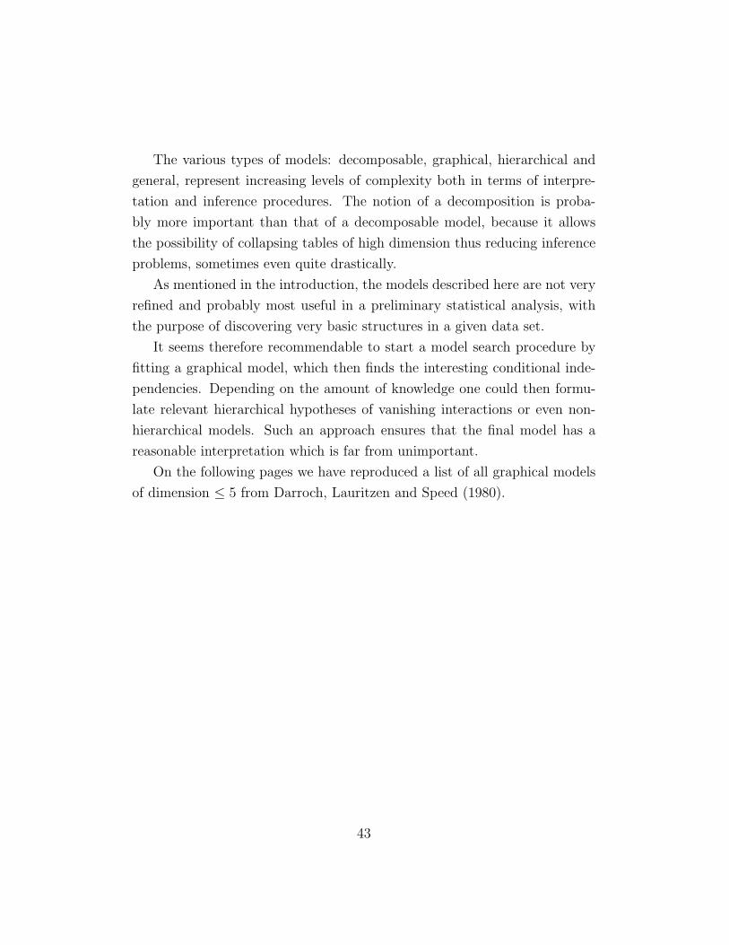
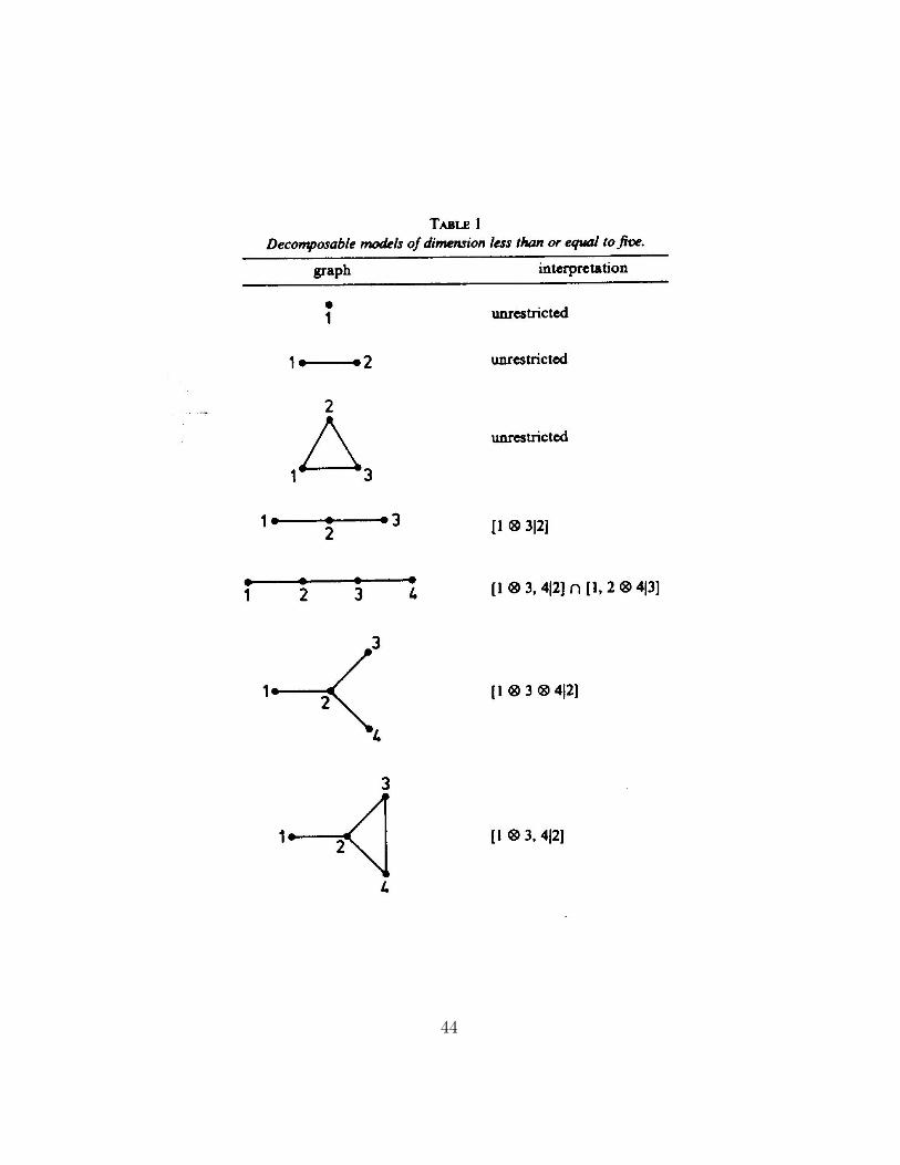
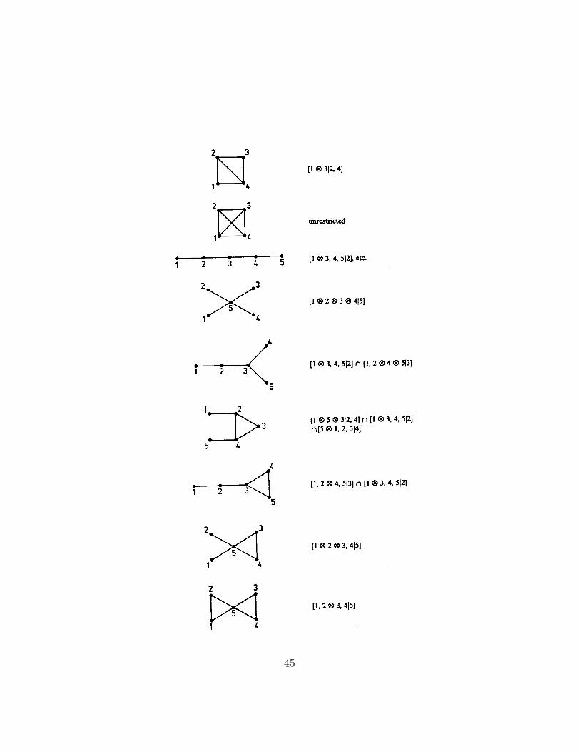
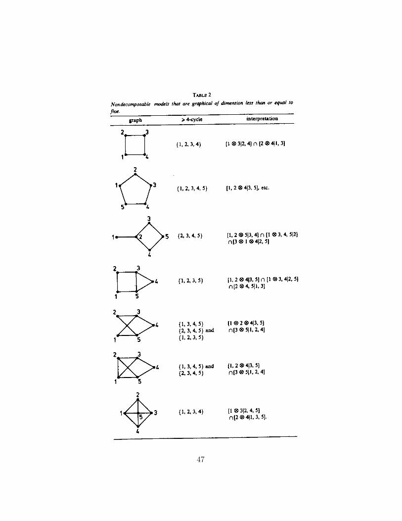
On the following pages we have reproduced a list of all graphical models

of dimension ≤ 5 from Darroch, Lauritzen and Speed (1980).

43

44

45

46

47

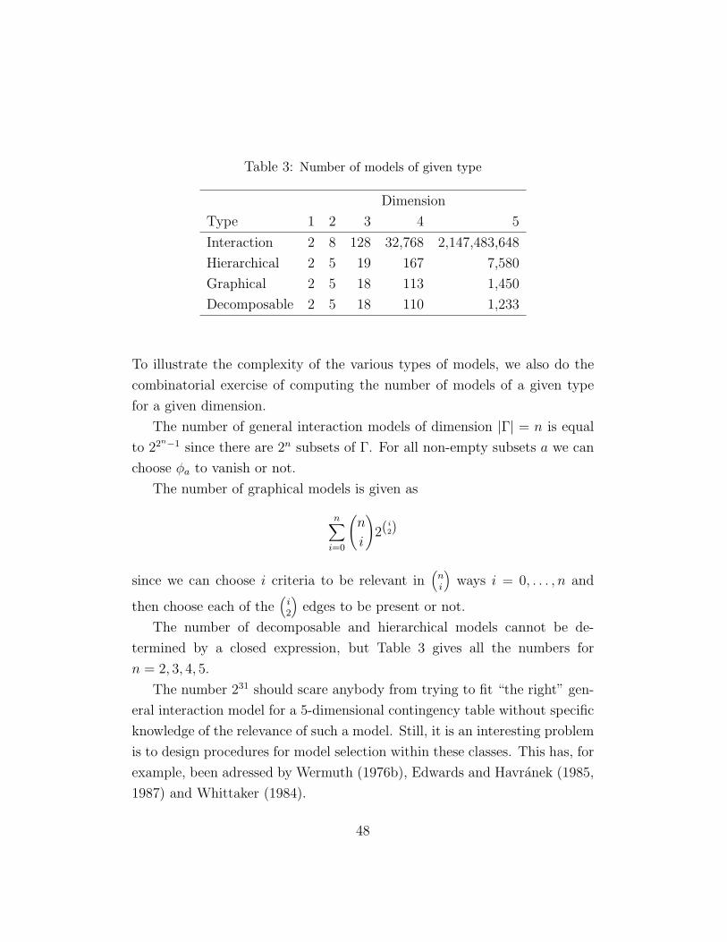
Table 3: Number of models of given type

Dimension

Type 1 2 3 4 5

Interaction 2 8 128 32,768 2,147,483,648

Hierarchical 2 5 19 167 7,580

Graphical 2 5 18 113 1,450

Decomposable 2 5 18 110 1,233

To illustrate the complexity of the various types of models, we also do the

combinatorial exercise of computing the number of models of a given type

for a given dimension.

The number of general interaction models of dimension |Γ| = n is equal

to 22n−1 since there are 2n subsets of Γ. For all non-empty subsets a we can

choose φa to vanish or not.

The number of graphical models is given as

n∑i=0

(n

i

)2(i

2)

since we can choose i criteria to be relevant in(ni

)ways i = 0, . . . , n and

then choose each of the(i2

)edges to be present or not.

The number of decomposable and hierarchical models cannot be de-

termined by a closed expression, but Table 3 gives all the numbers for

n = 2, 3, 4, 5.

The number 231 should scare anybody from trying to fit “the right” gen-

eral interaction model for a 5-dimensional contingency table without specific

knowledge of the relevance of such a model. Still, it is an interesting problem

is to design procedures for model selection within these classes. This has, for

example, been adressed by Wermuth (1976b), Edwards and Havranek (1985,

1987) and Whittaker (1984).

48

10 Analogies to covariance selection models

Models analogous to the graphical models exist also for the multivariate

normal distribution. These are the so-called covariance selection models

introduced by Dempster (1972).

Here X = XΓ is a vector of real-valued random variables indexed by Γ.

We assume that

X ∼ N(0,Σ), with Σ ∈ S(Γ,E)

where S(Γ,E) is the set of positive definite symmetric matrices such that

σαβ = 0 whenever α 6∼ β.

Here

Σ = {σαβ}, Σ−1 = {σαβ}.

Since we have for a normal distribution that

σαβ = 0 ⇔ Xα⊥⊥Xβ | XΓ\{α,β}

we see that this model is given by exactly the same type of conditional

independencies as our graphical models.

Further, since the multivariate distribution of a normal vector is com-

pletely specified by its ‘first-order interactions’ σαβ, there exist no ‘hierarchi-

cal’ models that are not graphical for this type.

If we have independent observations X(1), . . . , X(n), and form the em-

pirical covariance matrix S, we further have that the maximum likelihood

estimate of Σ is given by the equations:

Σ ∈ S(Γ,E), Σc = Sc ∀c ∈ C,

where C is the cliques of (Γ, E) and Σc, Sc are the marginals corresponding to

(Xγ, γ ∈ c). So for these models, the question of estimation is the question of

‘fitting the marginals’. An IPS-algorithm exists cf. Speed and Kiiveri (1986)

etc.

49

If the graph is decomposable, one can show that we have

Σ−1 =∑d

ν(d)[S−1d ]0

and that

det Σ =∏d

(det Σd)ν(d) ∀Σ ∈ S(Γ,E),

where [S−1d ]0 is the matrix obtained by inverting Sd, filling in the correspond-

ing elements and letting other elements be equal to zero and ν(d) is the index

mentioned in Section 5. A more detailed discussion of this can be found in

Wermuth (1976a).

Thus we see that the analogy to these models is much more direct than

that to models for the analysis of variance, where we make an expansion of

the expectation of a normal variate into its ‘interactions’.

Recently, the theory of contingency tables and covariance selection models

have been unified and extended to graphical association models for mixed

quantitative and categorical data. The basic theory for graphical models is

developed in Lauritzen and Wermuth (1989) and extended to hierarchical

models by Edwards (1990).

The models have also been extended to deal with situations where some

variables are responses and some explanatory. Wermuth and Lauritzen (1983,

1990) discuss for example this aspect.

A comprehensive exposition of these developments as well as further ref-

erences can be found in Lauritzen (1996).

References

Andersen, A. H. (1974). Multidimensional contingency tables. Scand. J.

Statist. 1, 115–127

Asmussen, S. and Edwards, D. (1983). Collapsibility and response variables

in contingency tables. Biometrika 70, 567–578

50

Bishop, Y. M. M., Fienberg, S.E. and Holland, P. W. (1975). Discrete Mul-

tivariate Analysis: Theory and Practice. MIT Press, Cambridge, Mass.

Barndorff-Nielsen, O. E. (1978). Information and Exponential Families in

Statistical Theory. Wiley, New York.

Brown, L. D. (1987). Fundamentals of Exponential Families with Applications

in Decision Theory. IMS Monographs, Vol. IX, California.

Darroch, J. N., Lauritzen S. L. and Speed, T. P. (1980). Markov-fields and

log-linear models for contingency tables. Ann. Statist. 8, 522–539

Darroch, J. N. and Speed, T. P. (1983). Additive and multiplicative models

and interactions. Ann. Statist. 11, 724–738

Dawid, A. P. (1979). Conditional independence in statistical theory (with

discussion). J. Roy. Statist. Soc. Ser. B 41, 1–31

Dawid, A. P. (1980). Conditional independence for statistical operations.

Ann. Statist. 8, 598–617

Dempster, A. P. (1972). Covariance selection. Biometrics 28, 157–175

Edwards, D. (1990). Hierarchical interaction models (with discussion). J.

Roy. Statist. Soc. Ser. B 52, 3–20 and 51–72

Edwards, D. and Havranek, T. (1985). A fast procedure for model search in

multidimensional contingency tables. Biometrika 72, 339–351

Edwards, D. and Havranek, T. (1987). A fast model selection procedure for

large families of models. J. Amer. Statist. Assoc. 82, 205–211

Haberman, S. J. (1974). The Analysis of Frequency Data. Univ. of Chicago

Press.

Isham, V. (1981). An introduction to spatial point processes and Markov

random fields. Int. Statist. Review 49, 21–43

Jensen, S. T. (1978). Flersidede kontingenstabeller. (Danish). Univ. Cop. Inst.

Math. Stat.

Johansen S. (1979). An Introduction to the Theory of Regular Exponential

Families. Lecture Notes 3, Univ. Cop. Inst. Math. Stat.

Kemeny, J. G., Snell, J. L., Knapp, A. W. and Griffeath, D. (1976). Denu-

merable Markov Chains. 2nd ed. Springer, Heidelberg.

51

Lauritzen, S. L. (1996). Graphical Models. Clarendon Press, Oxford.

Lauritzen, S. L., Speed, T. P. and Vijayan, K. (1984). Decomposable graphs

and hypergraphs. J. Austral. Math. Soc. A 36, 12–29

Lauritzen, S. L. and Spiegelhalter, D. J. (1988). Local computations with

probabilities on graphical structures and their application to expert sys-

tems (with discussion). J. Roy. Statist. Soc. Ser. B 50, 157–224

Lauritzen, S. L. and Wermuth, N. (1989). Graphical models for associations

between variables, some of which are qualitative and some quantitative.

Ann. Statist. 17, 31–57

Pearl, J. (1988). Probabilistic Inference in Intelligent Systems. Morgan Kauf-

mann, San Mateo.

Speed, T. P. (1978). Graph-theoretic methods in the analysis of interactions.

Mimeographed lecture notes. Univ. Cop. Inst. Math. Stat.

Speed, T. P. (1979). A note on nearest-neighbour Gibbs and Markov proba-

bilities. Sankhya A 41, 184–197

Speed, T. P. and Kiiveri, H. (1986). Gaussian Markov distributions over finite

graphs. Ann. Statist. 14, 138–150

Wermuth, N. (1976a). Analogies between multiplicative models in contin-

gency tables and covariance selection. Biometrics 32, 95–108

Wermuth, N. (1976b). Model search among multiplicative models. Biometrics

32, 253–263

Wermuth, N. and Lauritzen, S. L. (1983). Graphical and recursive models

for contingency tables. Biometrika 70, 537–552

Wermuth, N. and Lauritzen, S. L. (1990). On substantive research hypothe-

ses, conditional independence graphs and graphical chain models (with

discussion). J. Roy. Statist. Soc. Ser. B 52, 21–72

Whittaker, J. (1984). Fitting all possible decomposable and graphical models

to multiway contingency tables. In Havranek, T. (ed.). COMPSTAT 84,

98–108. Physica Verlag, Vienna.

52