lectures notes on string theory - sorbonne-universite.frisrael/notes.pdf · string theory proper...
TRANSCRIPT


Lucio Fontana, « Concetto Spaziale »

Foreword
These lecture notes are based upon a series of courses given at the master program ICFPfrom 2018 by the author. Comments and suggestions are welcome. Some references that cancomplement these notes are
• Superstring Theory (Green, Schwarz, Witten) [1,2]: the classic textbook from the eight-ies, naturally outdated on certain aspects but still an unvaluable reference on manytopics including the Green-Schwarz string and compactifications on special holonomymanifolds.
• String Theory (Polchinski) [3,4]: the standard textbook, with a very detailed derivationof the Polyakov path integral and strong emphasis on conformal field theory methods.
• String Theory in a Nutshell (Kiritsis) [5]: a concise presentation of string and super-string theory which moves quickly to rather advanced topics
• String Theory and M-Theory: A Modern Introduction (Becker, Becker, Schwarz) [6]:a good complement to the previous references, with a broad introduction to moderntopics as AdS/CFT and flux compactifications.
• A first course in String theory (Zwiebach) [7]: an interesting and different approach,making little use of conformal field theory methods, in favor of a less formal approach.
• Basic Concepts of String Theory (Blumenhagen, Lust, Theisen) [8]. As its name doesnot suggest, this book covers a lot of rather advanced topics about the worldsheetaspects of string theory. It is also rather appropriate for a math-oriented reader.
• The lectures notes of David Tong (http://www.damtp.cam.ac.uk/user/tong/string.html)are rather enjoyable to read, with a good balance between mathematical rigor and phys-ical intuition.
• The very lively online lectures of Shiraz Minwalla: http://theory.tifr.res.in/ minwalla/
Conventions
• The space-time metric is chosen to be of signature (−,+, . . . ,+).
• We work in units ~ = c = 1
Latest update
March 9, 2020
References
[1] M. B. Green, J. H. Schwarz, and E. Witten, Superstring theory, Vol. 1: Introduction.Cambridge Monographs on Mathematical Physics. 1988.
[2] M. B. Green, J. H. Schwarz, and E. Witten, Superstring theory, Vol. 2: loop amplitudes,anomalies and phenomenology. Cambridge, Uk: Univ. Pr. ( 1987) 596 P. ( CambridgeMonographs On Mathematical Physics), 1988.
[3] J. Polchinski, String theory. Vol. 1: An introduction to the bosonic string. CambridgeUniversity Press, 2007.
[4] J. Polchinski, String theory. Vol. 2: Superstring theory and beyond. Cambridge UniversityPress, 2007.
[5] E. Kiritsis, String theory in a nutshell. Princeton, USA: Univ. Pr. (2007) 588 p, 2007.
[6] K. Becker, M. Becker, and J. H. Schwarz, String theory and M-theory: A modern intro-duction. Cambridge University Press, 2006.
[7] B. Zwiebach, A first course in string theory. Cambridge University Press, 2006.
[8] R. Blumenhagen, D. Lust, and S. Theisen, Basic concepts of string theory. Theoreticaland Mathematical Physics. Springer, Heidelberg, Germany, 2013.
2

Contents
1 Introduction 51.1 Gravity and quantum field theory . . . . . . . . . . . . . . . . . . . . . . . . . 61.2 String theory: historical perspective . . . . . . . . . . . . . . . . . . . . . . . . 10
2 Bosonic strings: action and path integral 152.1 Relativistic particle in the worldline formalism . . . . . . . . . . . . . . . . . . 162.2 Relativistic strings . . . . . . . . . . . . . . . . . . . . . . . . . . . . . . . . . 252.3 Symmetries . . . . . . . . . . . . . . . . . . . . . . . . . . . . . . . . . . . . . 302.4 Polyakov path integral . . . . . . . . . . . . . . . . . . . . . . . . . . . . . . . 392.5 Open strings . . . . . . . . . . . . . . . . . . . . . . . . . . . . . . . . . . . . . 45
3 Conformal field theory 523.1 The conformal group in diverse dimensions . . . . . . . . . . . . . . . . . . . . 543.2 Radial quantization . . . . . . . . . . . . . . . . . . . . . . . . . . . . . . . . . 553.3 Conformal invariance and Ward identities . . . . . . . . . . . . . . . . . . . . 583.4 Primary operators . . . . . . . . . . . . . . . . . . . . . . . . . . . . . . . . . . 623.5 The Virasoro Algebra . . . . . . . . . . . . . . . . . . . . . . . . . . . . . . . . 663.6 The Weyl anomaly . . . . . . . . . . . . . . . . . . . . . . . . . . . . . . . . . 733.7 Conformal field theory with boundaries . . . . . . . . . . . . . . . . . . . . . . 75
4 Free conformal field theories 774.1 Free scalar fields . . . . . . . . . . . . . . . . . . . . . . . . . . . . . . . . . . 784.2 Free fermions . . . . . . . . . . . . . . . . . . . . . . . . . . . . . . . . . . . . 914.3 The ghost CFT . . . . . . . . . . . . . . . . . . . . . . . . . . . . . . . . . . . 101
5 The string spectrum 1075.1 String theory and the dimension of space-time . . . . . . . . . . . . . . . . . . 1085.2 BRST quantization . . . . . . . . . . . . . . . . . . . . . . . . . . . . . . . . . 1115.3 The closed string spectrum . . . . . . . . . . . . . . . . . . . . . . . . . . . . . 1235.4 Open string spectrum . . . . . . . . . . . . . . . . . . . . . . . . . . . . . . . . 1285.5 Physical degrees of freedom and light-cone gauge . . . . . . . . . . . . . . . . 1335.6 General structure of the string spectrum . . . . . . . . . . . . . . . . . . . . . 136
3
6 String interactions 1406.1 The string S-matrix . . . . . . . . . . . . . . . . . . . . . . . . . . . . . . . . . 1416.2 Four-tachyon tree-level scattering . . . . . . . . . . . . . . . . . . . . . . . . . 1426.3 One-loop partition function . . . . . . . . . . . . . . . . . . . . . . . . . . . . 149
7 Introduction to superstring theories 1607.1 Two-dimensional local supersymmetry . . . . . . . . . . . . . . . . . . . . . . 1617.2 Superconformal symmetry . . . . . . . . . . . . . . . . . . . . . . . . . . . . . 1697.3 BRST quantization . . . . . . . . . . . . . . . . . . . . . . . . . . . . . . . . . 1767.4 Type II superstring theories . . . . . . . . . . . . . . . . . . . . . . . . . . . . 1837.5 One-loop vacuum amplitudes . . . . . . . . . . . . . . . . . . . . . . . . . . . 189
4

Chapter 1
Introduction
5

Introduction.
In Novembrer 1994, Joe Polchinski published on the ArXiv repository a preliminary ver-sion of his celebrated textbook on String theory, based on lectures given at Les Houches,under the title ”What is string theory?” [1]. If he were asked the same question today, theanswer would probably be rather different as the field has evolved since in various directions,some of them completely unexpected at the time.
One may try to figure out what string theory is about by looking at the program of Strings2017, the last of a series of annual international conferences about string theory that havetaken place at least since 1989, all over the world. Among the talks less than half were aboutstring theory proper (i.e. the theory you will read about in these notes) while the otherspertained to a wide range of topics, such as field theory amplitudes, dualities in field theory,theoretical condensed matter or general relativity.
The actual answer to the question raised by Joe Polchinski, ”What is string theory?”, maybe answered at different levels:
• litteral: the quantum theory of one-dimensional relativistic objects that interact byjoining and splitting.
• historical: before 1974, a candidate theory of strong interactions; after that date, aquantum theory of gravity.
• practical: a non-perturbative quantum unified theory of fundamental interactions whosedegrees of freedom, in certain perturbative regime, are given by relativistic strings.
• sociological: a subset of theoretical physics topics studied by people that define them-selves as doing research in string theory.
In these notes, we will provide the construction of a consistent first quantized theory ofinteracting quantum closed strings. We will show that such theory automatically includes a(perturbative) theory of quantum gravity. We will introduce also open strings that incorpo-rate gauge interactions, and give rise to the concept of D-branes that plays a prominent rolein the AdS/CFT correspondence.
Along the way we will introduce some concepts and techniques that are as useful in otherareas of theoretical physics as they are in string theory, for instance conformal field theories,BRST quantization of gauge theories or supersymmetry.
1.1 Gravity and quantum field theory
String theory has been investigated by a significant part of the high-energy theory communityfor more than forty years as it provides a compelling answer – and maybe the answer – tothe following outstanding question: what is the quantum theory of gravity?
A successful theory of quantum gravity from the theoretical physics viewpoint should atleast satisfy the following properties:
6

Introduction.
1. the theory should reproduce general relativity, in an appropriate classical, low-energyregime;
2. the theory should be renormalizable or better UV-finite in order to have predictivepower;
3. it should satisfy the basic requirements for any quantum theory, such as unitarity;
4. it should explain the origin of black hole entropy, possibly the only current predictionfor quantum gravity;
5. last but not least, the physical predictions should be compatible with experiments, inparticular with the Standard Model of particle physics, astrophysical and cosmologicalobservations.
According to our current understanding, string theory passes successfully the first fourtests. Whether string theory reproduces accurately at energies accessible to experiments theknown physics of fundamental particles and interaction is still unclear, given that such physicsoccurs in a regime of the theory that is beyond our current analytical control (to draw ananalogy, one cannot reproduce analytically the physics of condensed matter systems from themicroscopic quantum mechanical description in terms of atoms). At least it is clear that themain ingredients are there: chiral fermions, non-Abelian gauge interactions and Higgs-likebosons.
The problem with quantizing general relativity
The classical theory of relativistic gravity in four space-time dimensions, or Einstein theory,follows in the absence of matter from the Einstein-Hilbert (EH) action in four space-timedimensions, that takes the form
Seh =1
2κ2
∫M
d4x√
− detg (R(g) − 2Λ) , (1.1)
where R is the Ricci scalar associated with the space-time manifold M, endowed with a met-ric g, and Λ the cosmological constant that has no a priori reason to vanish. The couplingconstant κ of the theory is related to the Newton’s constant through κ =
√8πG; by dimen-
sional analysis it has dimension of length. Its inverse defines the Planck massMPl ∼ 1019 GeV.
Quantizing general relativity raises a number of deep conceptual issues, that can be raisedeven before attempting to make any explicit computation. Some of them are:
• Because of diffeormorphism invariance, there are no local observables in general relativ-ity.
• A path-integral formulation of quantum gravity should include, by definition, a sumover space-time geometries. Which geometries should be considered? Should we specifyboundary conditions?
7

Introduction.
• A Hamiltonian formulation of quantum gravity would require a foliation of space-timein terms of space-like hypersurfaces. Generically, such foliation does not exist.
• Classical dynamics of general relativity predicts the formation of event horizons, shield-ing regions of space-time from the exterior. This challenges the unitarity of the theory,through the black hole information paradox.
Quantum gravity with a positive cosmological constant – which seems to be relevant to de-scribe the Universe – raises a number of additional conceptual issues that will be ignoredin the rest of the lectures. We will mainly focus on theories with a vanishing cosmologi-cal constant; the case of negative cosmological constant will be discussed in the AdS/CFTlectures.
Perturbative QFT for gravity
One may try to ignore these conceptual problems and build a quantum field theory of gravityin the usual way, i.e. by defining propagators, vertices, Feynman rules, etc..., from thenon-linear EH action, eqn. (1.1) [2].
With vanishing cosmological constant, one considers fluctuations of the metric around areference Minkowski space-time metric:
gµν = ηµν + hµν . (1.2)
Linearizing the equations of motion that follows from (1.1), in the absence of sources, wearrive to:
hµν − 2∂ρ∂(µhν)ρ + η
µν∂ρ∂σhµν = 0 , (1.3)
where we have defined the ”trace-reversed” tensor hµν = hµν−12hρρ ηµν. This theory possesses
a gauge invariance that comes from the diffeomorphism invariance of the full theory. Theequations of motion are invariant under
hµν 7→ hµν + ∂µζν + ∂νζµ . (1.4)
One can choose to work in a Lorentz gauge, defined by ∂µhµν = 0, in which case the fieldequations (1.3) amounts to a wave equation for each component, hµν = 0.
The solutions of these equations are naturally plane waves hµν(xρ) = h0µν exp(ikρx
ρ), andthe Lorentz gauge condition means that they are transverse. Finally, the residual gaugeinvariance that remains in the Lorentz gauge, corresponding to vector fields ζµ satisfying thewave equation ζµ = 0, can be fixed by choosing the longitudinal gauge h0µ = 0. As a result,the gravitational waves have two independent transverse polarizations. The correspondingquantum theory is a theory of free gravitons that are massless bosons of helicity two.
The interactions between gravitons are added by expanding the EH action around thebackground (1.2) in powers of hµν. In pure gravity one obtains three-graviton and four-graviton vertices, that have a rather complicated form. For instance the four-graviton vertex
8
Introduction.
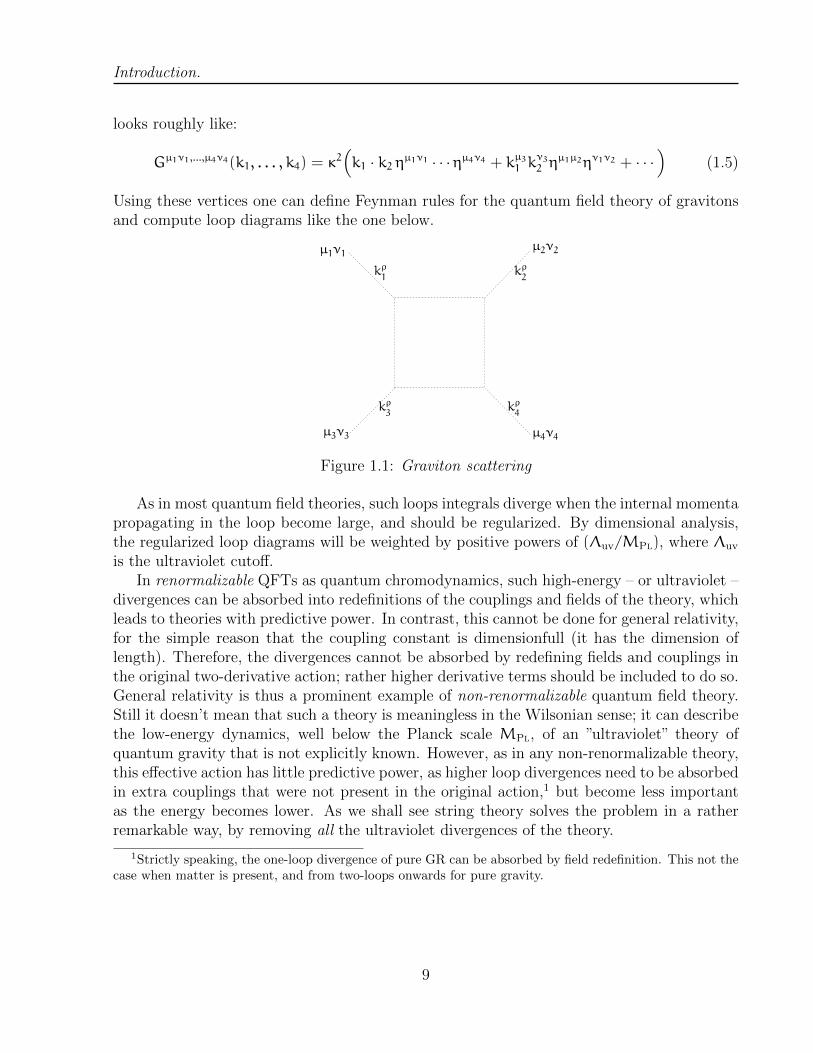
looks roughly like:
Gµ1ν1,...,µ4ν4(k1, . . . , k4) = κ2(k1 · k2 ηµ1ν1 · · ·ηµ4ν4 + kµ31 k
ν32 η
µ1µ2ην1ν2 + · · ·)
(1.5)
Using these vertices one can define Feynman rules for the quantum field theory of gravitonsand compute loop diagrams like the one below.
µ3ν3
µ1ν1µ2ν2
µ4ν4
kρ2
kρ1
kρ3
kρ4
Figure 1.1: Graviton scattering
As in most quantum field theories, such loops integrals diverge when the internal momentapropagating in the loop become large, and should be regularized. By dimensional analysis,the regularized loop diagrams will be weighted by positive powers of (Λuv/MPl), where Λuv
is the ultraviolet cutoff.In renormalizable QFTs as quantum chromodynamics, such high-energy – or ultraviolet –
divergences can be absorbed into redefinitions of the couplings and fields of the theory, whichleads to theories with predictive power. In contrast, this cannot be done for general relativity,for the simple reason that the coupling constant is dimensionfull (it has the dimension oflength). Therefore, the divergences cannot be absorbed by redefining fields and couplings inthe original two-derivative action; rather higher derivative terms should be included to do so.General relativity is thus a prominent example of non-renormalizable quantum field theory.Still it doesn’t mean that such a theory is meaningless in the Wilsonian sense; it can describethe low-energy dynamics, well below the Planck scale MPl, of an ”ultraviolet” theory ofquantum gravity that is not explicitly known. However, as in any non-renormalizable theory,this effective action has little predictive power, as higher loop divergences need to be absorbedin extra couplings that were not present in the original action,1 but become less importantas the energy becomes lower. As we shall see string theory solves the problem in a ratherremarkable way, by removing all the ultraviolet divergences of the theory.
1Strictly speaking, the one-loop divergence of pure GR can be absorbed by field redefinition. This not thecase when matter is present, and from two-loops onwards for pure gravity.
9

Introduction.
1.2 String theory: historical perspective
This is a very sketchy account about the history of string theory; interested reader mayconsult the book [3] for first-hand testimonies.
String theory as a theory of quantum gravity came almost by accident, after being pro-posed as a theory of strong interactions. The prehistory of string theory occurred during thesixties. At that time, general relativity was not, with few exceptions, a topic of interest fortheoretical physicists, but was rather a playground for mathematicians.
Quantum field theory itself didn’t have the central role that it has today in our under-standing of fundamental interactions. While quantum electrodynamics was acknowledged asthe appropriate description of electromagnetic interactions, most physicists thought that itwas an inappropriate tool to solve the big problems of the time, the physics of strong andweak interactions. This was especially true for the strong interactions, as the experimentswere finding a growing number of hadronic particles, with large masses and spins. Theseparticles were mostly resonances i.e. particles with a finite lifetime. Defining a QFT includ-ing all of these resonances did not seem, rightfully, a sensible idea. Quarks did make theirappearance in the theoretical physicists’ lexicon, however they were thought as mathemati-cal tools rather than as actual elementary particles – the fact that they cannot be observedindividually supported this point of view.
A different approach, called the S-matrix program, was widely popular back then. The ideawas to construct directly the S-matrix of the theory using some general physical principles(unitarity, analyticity,...), as well as some experimental input from the specific theory thatwas considered, without any reference to a ”microscopic” Lagrangian.
One crucial experimental observation was that hadronic resonances could be classified infamilies along curves in the mass-angular momentum plane (M, J) called Regge trajectories:
J = α(0) + α ′M2 (1.6)
The value of the parameter α(0), or intercept, was determining a given family of resonances,while the slope α ′ was universal – with one exception – and given experimentally by
α ′ ' 1GeV−2 (1.7)
in natural units.
Figure 1.2: Channel duality: s-channel (left) and t-channel (right)
Among important requirements imposed upon the S-matrix, was that all the hadronsalong the Regge trajectories should appear on the same footing, and both as intermediate
10
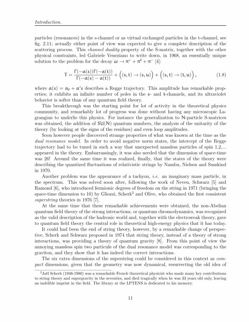
Introduction.
particles (resonances) in the s-channel or as virtual exchanged particles in the t-channel, seefig. 2.11; actually either point of view was expected to give a complete description of thescattering process. This channel duality property of the S-matrix, together with the otherphysical constraints, led Gabriele Veneziano to write down, in 1968, an essentially uniquesolution to the problem for the decay ω→ π+ + π0 + π− [4]:
T =Γ(−α(s))Γ(−α(t))
Γ(−α(s) − α(t))+((s, t)→ (s, u)
)+((s, t)→ (t, u)
), (1.8)
where α(s) = α0 + α′s describes a Regge trajectory. This amplitude has remarkable prop-
erties; it exhibits an infinite number of poles in the s- and t-channels, and its ultravioletbehavior is softer than of any quantum field theory.
This breakthrough was the starting point for lot of activity in the theoretical physicscommunity, and remarkably lot of progress was done without having any microscopic La-grangian to underlie this physics. For instance the generalization to N-particle S-matriceswas obtained, the addition of SU(N) quantum numbers, the analysis of the unitarity of thetheory (by looking at the signs of the residues) and even loop amplitudes.
Soon however people discovered strange properties of what was known at the time as thedual resonance model. In order to avoid negative norm states, the intercept of the Reggetrajectory had to be tuned in such a way that unexpected massless particles of spin 1,2,...appeared in the theory. Embarrassingly, it was also needed that the dimension of space-timewas 26! Around the same time it was realized, finally, that the states of the theory weredescribing the quantized fluctuations of relativistic strings by Nambu, Nielsen and Susskindin 1970.
Another problem was the appearance of a tachyon, i.e. an imaginary mass particle, inthe spectrum. This was solved soon after, following the work of Neveu, Schwarz [5] andRamond [6], who introduced fermionic degrees of freedom on the string in 1971 (bringing thespace-time dimension to 10) by Gliozzi, Scherk2 and Olive, who obtained the first consistentsuperstring theories in 1976 [7].
At the same time that these remarkable achievements were obtained, the non-Abelianquantum field theory of the strong interactions, or quantum chromodynamics, was recognizedas the valid description of the hadronic world and, together with the electroweak theory, gaveto quantum field theory the central role in theoretical high-energy physics that it has today.
It could had been the end of string theory, however, by a remarkable change of perspec-tive, Scherk and Schwarz proposed in 1974 that string theory, instead of a theory of stronginteractions, was providing a theory of quantum gravity [8]. From this point of view theannoying massless spin two particule of the dual resonance model was corresponding to thegraviton, and they show that it has indeed the correct interactions.
The six extra dimensions of the superstring could be considered in this context as com-pact dimensions, given that the geometry was now dynamical, resurrecting the old idea of
2Joel Scherk (1946-1980) was a remarkable French theoretical physicist who made many key contributionsto string theory and supergravity in the seventies, and died tragically when he was 33 years old only, leavingan indelible imprint in the field. The library at the LPTENS is dedicated to his memory.
11

Introduction.
Kaluza [9], and Klein [10] from the twenties. The value of the Regge slope should be radicallydifferent from was it was considered before in the hadronic context, in order to account forthe observed magnitude of four-dimensional gravity. One was considering
α ′ ' 10−38Gev−2 , (1.9)
or equivalently strings of a size smaller by 19 orders of magnitude than the hadronic string,i.e. impossible to resolve directy by current or foreseeable experiments. Despite that stringtheory was able to fullfill an old dream – quantizing general relativity – research in stringtheory remained rather confidential before the next turning point of its history,
Between 1984 and 1986, several important discoveries occurred and changed the fate ofthe theory: the invention of heterotic string [11] (which made easy to incorporate non-Abeliangauge interactions in string theory), the Green-Schwarz anomaly cancellation mechanism [12]which strengthened the link between string theory and low-energy supergravity, thereby mak-ing the former more convincing, and finally the discovery of Calabi-Yau compactifications [13]and orbifold compactifications [14] which allowed to get at low energies models of particlephysics with N = 1 supersymmetry in four dimensions. After that string theory becamemore mainstream, as many theoretical physicists started to realize that it was a promisingway of unifying all fundamental particles and interactions in a consistent quantum theory.
Thirty years and a second revolution after, we haven’t yet achieved this goal fully buttremendous progress has been made, the hallmarks being the discoveries of D-branes [15], ofstrong/weak dualities [16–18], of holographic dualities [19] and of flux compactifications [20,21] to name a few. We still have a long way to go, and it is certainly worth trying.
References
[1] J. Polchinski, “What is string theory?,” in NATO Advanced Study Institute: Les HouchesSummer School, Session 62: Fluctuating Geometries in Statistical Mechanics and FieldTheory Les Houches, France, August 2-September 9, 1994. 1994. hep-th/9411028.
[2] S. Weinberg, “Ultraviolet divergences in quantum theories of gravitation.,” in GeneralRelativity: An Einstein centenary survey, S. W. Hawking and W. Israel, eds., pp. 790–831. 1979.
[3] M. Gasperini and J. Maharana, “String theory and fundamental interactions,” Lect.Notes Phys. 737 (2008) pp.1–974.
[4] G. Veneziano, “Construction of a crossing - symmetric, Regge behaved amplitude forlinearly rising trajectories,” Nuovo Cim. A57 (1968) 190–197.
[5] A. Neveu and J. H. Schwarz, “Factorizable dual model of pions,” Nucl. Phys. B31 (1971)86–112.
[6] P. Ramond, “Dual Theory for Free Fermions,” Phys. Rev. D3 (1971) 2415–2418.
12

Introduction.
[7] F. Gliozzi, J. Scherk, and D. I. Olive, “Supergravity and the Spinor Dual Model,” Phys.Lett. 65B (1976) 282–286.
[8] J. Scherk and J. H. Schwarz, “Dual Models for Nonhadrons,” Nucl. Phys. B81 (1974)118–144.
[9] T. Kaluza, “On the Problem of Unity in Physics,” Sitzungsber. Preuss. Akad. Wiss.Berlin (Math. Phys.) 1921 (1921) 966–972.
[10] O. Klein, “Quantum Theory and Five-Dimensional Theory of Relativity. (In Germanand English),” Z. Phys. 37 (1926) 895–906. [Surveys High Energ. Phys.5,241(1986)].
[11] D. J. Gross, J. A. Harvey, E. J. Martinec, and R. Rohm, “The Heterotic String,” Phys.Rev. Lett. 54 (1985) 502–505.
[12] M. B. Green and J. H. Schwarz, “Anomaly Cancellation in Supersymmetric D=10 GaugeTheory and Superstring Theory,” Phys. Lett. 149B (1984) 117–122.
[13] P. Candelas, G. T. Horowitz, A. Strominger, and E. Witten, “Vacuum Configurationsfor Superstrings,” Nucl. Phys. B258 (1985) 46–74.
[14] L. J. Dixon, J. A. Harvey, C. Vafa, and E. Witten, “Strings on Orbifolds,” Nucl. Phys.B261 (1985) 678–686.
[15] J. Polchinski, “Dirichlet Branes and Ramond-Ramond charges,” Phys. Rev. Lett. 75(1995) 4724–4727, hep-th/9510017.
[16] A. Sen, “Strong - weak coupling duality in four-dimensional string theory,” Int. J. Mod.Phys. A9 (1994) 3707–3750, hep-th/9402002.
[17] C. M. Hull and P. K. Townsend, “Unity of superstring dualities,” Nucl. Phys. B438(1995) 109–137, hep-th/9410167.
[18] E. Witten, “String theory dynamics in various dimensions,” Nucl. Phys. B443 (1995)85–126, hep-th/9503124.
[19] J. M. Maldacena, “The Large N limit of superconformal field theories and supergrav-ity,” Int. J. Theor. Phys. 38 (1999) 1113–1133, hep-th/9711200. [Adv. Theor. Math.Phys.2,231(1998)].
[20] K. Dasgupta, G. Rajesh, and S. Sethi, “M theory, orientifolds and G - flux,” JHEP 08(1999) 023, hep-th/9908088.
[21] S. B. Giddings, S. Kachru, and J. Polchinski, “Hierarchies from fluxes in string compact-ifications,” Phys. Rev. D66 (2002) 106006, hep-th/0105097.
13

Introduction.
14

Chapter 2
Bosonic strings: action and pathintegral
15

Bosonic strings: action and path integral
Bosonic string theory, which is the most basic form of string theory, describes the prop-agation of one-dimensional relativistic extended objects, the fundamental strings, and theirinteractions by joining and splitting.
Quantum field theories of point particles are obtained by starting with a classical action,and quantizing the fluctuations around a given classical solution of the equations of motion.Upon quantization one gets field operators acting on the Fock space of the theory by creatingor annihilating particles at a given point in space. An analogous string field theory exists,but is still poorly understood. In such theory one should have operators creating a loop inspace, which is certainly more difficult to describe mathematically.
Rather the practical way to handle string theory is to follow the propagation in time of asingle string in a fixed reference space-time. As restrictive as it looks like, this first-quantizedformalism does not prevent for studying the interactions between strings, computing loopamplitudes and make a large number of predictions. As we will see below this ”first-order”formalism can be used for point particles as well, as an alternative to QFT Feynman diagramsthat allows to perform perturbative computations; however it misses important aspects assolitons or instantons that can be handled semi-classically from a field theory, and is notsuited for all types of computations.
2.1 Relativistic particle in the worldline formalism
We consider a relativistic particle of mass m and charge q in a given d-dimensional space-time M of metric G and background electromagnetic field. Its dynamics is governed by theaction
S = −m
∫l
ds− q
∫l
A , (2.1)
where l is the worldline of the particle, s the proper time and A(xµ) = A(xµ)ρdxρ the gauge
potential. Under a gauge transformation, A 7→ A+dΛ, the worldline action (2.1) is invariantup to possible boundary terms.
The worldline of the particle in space-time M corresponds to an embedding map1
R → M (2.2)
τ 7→ xµ(τ) , (2.3)
where τ is an affine parameter and xµ, µ = 0, . . . , D − 1 a set of coordinates on M. Theproper time differential can be expressed as
ds2 = −Gµνxµxνdτ 2 , (2.4)
therefore the action (2.1) can be rewritten as
S = −m
∫dτ√
−xµ(τ)xν(τ)Gµν[xρ(τ)] − q
∫l
Aµ[xµ(τ)]dxµ(τ) . (2.5)
1Strictly speaking, this is in general valid in an open set ofM where the coordinates xµ, µ = 0, . . . , D−1are well-defined.
16
Bosonic strings: action and path integral
This action is invariant under diffeomorphisms of the worldline, i.e. under any differentiablereparametrization
τ 7→ τ(τ) (2.6)
The embedding is now given by definition by the set of differentiable functions xµ(τ) =xµ(τ), µ = 0, . . . , D− 1.
Let us consider the variation of the particle action (2.5) under the infinitesimal change ofthe path, namely
xµ 7→ xµ + δxµ (2.7a)
Gµν 7→ Gµν + ∂σGµνδxσ . (2.7b)
At first order, one gets
δS = m
∫dτ
Gµσx
µδxσ√−xµxνGµν
+xµxν∂σGµνδx
σ√−xµxνGµν
−q
m(Aσδx
σ + ∂σAµδxρxµ)
(2.8)
After integration by parts of the first and third term, and trading the integral over the affineparmeter τ for the integral over the proper time s, one gets
δS = m
∫ds
[d2xν
ds2+ Γνρσ
dxρ
ds
dxσ
ds−q
mFνµ
dxµ
ds
]δxν (2.9)
Not surprisingly, one obtains the relativistic equation of motion of a massless charged particle,i.e. the geodesic equation plus the coupling to the electromagnetic field strength F = dA.
In order to make more explicit the diffeomorphism invariance of the worldline action, onecan introduce an independent worldline metric as ds2 = −hττ(τ)dτ
2. In the one-dimensionalanalogue of the tetrad formalism of general relativity, one defines the einbein e(τ) =
√−hττ.
The action (2.5) can be then rewritten in a classically equivalent way as:
Se = −1
2
∫dτ√
−hττ(hττ∂τx
µ∂τxνGµν +m
2)− q
∫l
Aµdxµ
=1
2
∫dτ
(1
eGµνx
µxν −m2e
)− q
∫l
Aµdxµ (2.10)
where one can see that e(τ) play the role of a Lagrange multiplier field e(τ) – i.e. a non-dynamical field that enforces a constraint in field space. Its equation of motion is simply0 = −e−2Gµνx
µxν −m2, which, upon replacing e by the solution in the action (2.10), givesback the original action (2.5).
One can view this action as a one-dimensional theory of gravity coupled to a set of freescalar fields xµ(t) (there is naturally no curvature term in one dimension). Notice thatthe coupling of the particle to the electromagnetic four-potential A – the last term in equa-tion (2.10) – is independent of the worldline metric. In this sense this coupling is of topologicalnature. Under diffeorphisms τ 7→ τ(τ) the einbein transforms according to
e(τ)dτ = e(τ)dτ (2.11)
17
Bosonic strings: action and path integral
which gives, for an infinitesimal transformation
τ 7→ τ = τ+ ε(τ) (2.12)
e(τ) 7→ e(τ) = e(τ) −d
dτ
(e(τ)ε(τ)
). (2.13)
As in four-dimensional gravity, this reparametrization invariance is a gauge symmetry, i.e.a redundancy in the description of the system that will eventually remove some degrees offreedom from the theory.2
Path integral quantization
The quadratic action (2.10) for the relativistic charged particle is a convenient starting pointfor quantizing the theory through the path integral formalism. It is convenient as well toanalytically continue the space-time to Euclidean signature x0 7→ ix0, as well as the worldlinetime τ 7→ iτ. We will consider a particle moving in flat space, i.e. with metric Gµν = δµν, inthe absence of electromagnetic field.
The one-particle vacuum energy in Euclidean space deduced from the wordline actionis given by summing over closed paths of the particle, which is given schematically by thefunctional integral:
Z1 =
∫De
Vol(diff)
∫x(0)=x(1)
Dx exp
−1
2
∫ 10
dτ
(1
ex2 +m2e
), (2.14)
where one has to divide the functional integral over the einbein (or equivalently over the one-dimensional metrics) by the infinite volume of the group of diffeomorphisms of the worldline.This group contains the transformations of the vielbein given infinitesimally by (2.13). Ontop of this shifts of τ by a constant, τ 7→ τ + τ0, are diffeomorphisms that are not fixed bythe choice of a reference einbein. The volume of this factor of the gauge group is finite andgiven by T , the invariant length of the closed path of the particle, see eq. (2.16) below. Wechoose finally the parameter τ to be in the interval [0, 1], and, the path being closed, theeinbein is a periodic function: e(τ+ 1) = e(τ).
Gauge symmetry
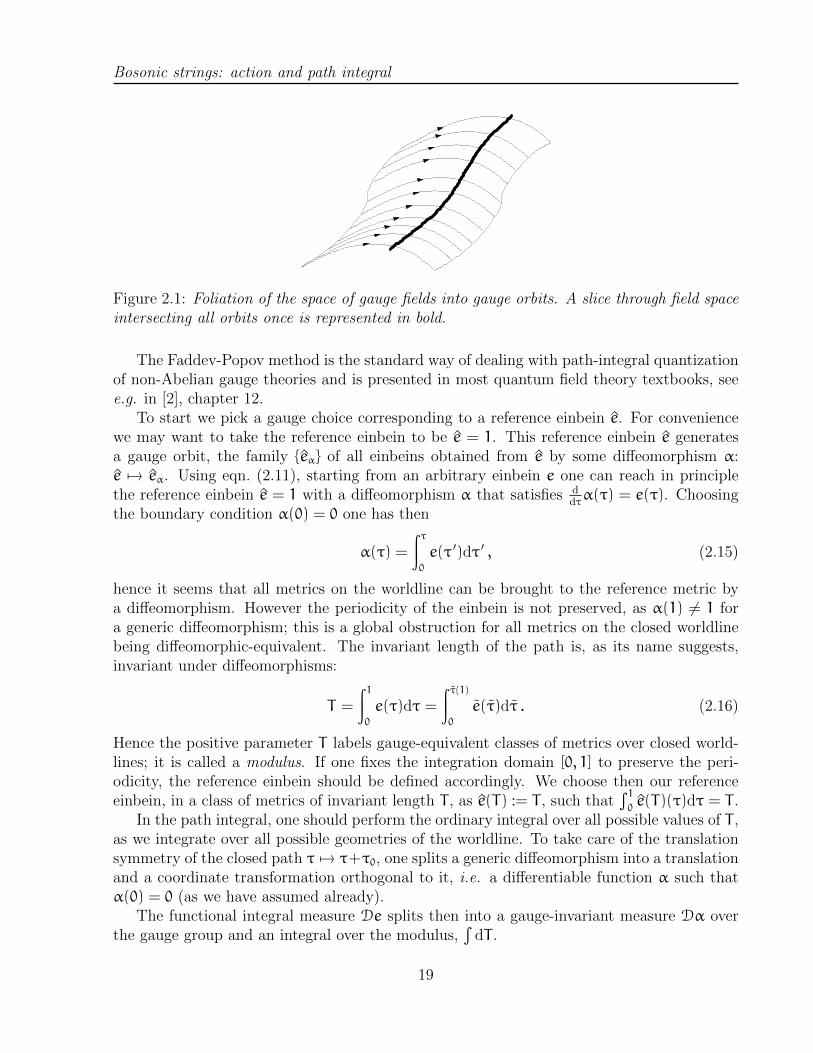
To carry the functional integral over the ”gauge field”e(τ) one starts by slicing the field spaceinto gauge orbits, i.e. einbeins that are related to each other by a diffeomorphism. The ratioof the integral over the whole field space over the volume of the group of diffeomorphismsis then equivalent to a functional integral over a slice in field space that cuts once eachorbit, see figure 2.1 up to the Jacobian of the change of coordinates in field space; this is theFaddeev-Popov method [1] (FP for short).3
2This redundancy was already explicit in the original description of the theory, eq. (2.1), as one couldhave chosen the gauge x0(τ) = τ to start with.
3This method is rather overkill for dealing with a free particle but will be used again in the case of thestring.
18
Bosonic strings: action and path integral
Figure 2.1: Foliation of the space of gauge fields into gauge orbits. A slice through field spaceintersecting all orbits once is represented in bold.
The Faddev-Popov method is the standard way of dealing with path-integral quantizationof non-Abelian gauge theories and is presented in most quantum field theory textbooks, seee.g. in [2], chapter 12.
To start we pick a gauge choice corresponding to a reference einbein e. For conveniencewe may want to take the reference einbein to be e = 1. This reference einbein e generatesa gauge orbit, the family eα of all einbeins obtained from e by some diffeomorphism α:e 7→ eα. Using eqn. (2.11), starting from an arbitrary einbein e one can reach in principlethe reference einbein e = 1 with a diffeomorphism α that satisfies d
dτα(τ) = e(τ). Choosing
the boundary condition α(0) = 0 one has then
α(τ) =
∫ τ0
e(τ ′)dτ ′ , (2.15)
hence it seems that all metrics on the worldline can be brought to the reference metric bya diffeomorphism. However the periodicity of the einbein is not preserved, as α(1) 6= 1 fora generic diffeomorphism; this is a global obstruction for all metrics on the closed worldlinebeing diffeomorphic-equivalent. The invariant length of the path is, as its name suggests,invariant under diffeomorphisms:
T =
∫ 10
e(τ)dτ =
∫ τ(1)0
e(τ)dτ . (2.16)
Hence the positive parameter T labels gauge-equivalent classes of metrics over closed world-lines; it is called a modulus. If one fixes the integration domain [0, 1] to preserve the peri-odicity, the reference einbein should be defined accordingly. We choose then our referenceeinbein, in a class of metrics of invariant length T , as e(T) := T , such that
∫10e(T)(τ)dτ = T .
In the path integral, one should perform the ordinary integral over all possible values of T ,as we integrate over all possible geometries of the worldline. To take care of the translationsymmetry of the closed path τ 7→ τ+τ0, one splits a generic diffeomorphism into a translationand a coordinate transformation orthogonal to it, i.e. a differentiable function α such thatα(0) = 0 (as we have assumed already).
The functional integral measure De splits then into a gauge-invariant measure Dα overthe gauge group and an integral over the modulus,
∫dT .
19

Bosonic strings: action and path integral
As in ordinary gauge theories like quantum chromodynamics in four space-time dimen-sions, one introduces then the Faddeev-Popov determinant through the relation:
1
∆fp(e):=
∫dT
∫Dαδ(e− eα(T))δ(α(0)) , (2.17)
The distribution δ(e − eα(T)) will eventually project the integral over the metrics ontoan integral over the chosen gauge slice in field space, which is a one-parameter family ofdiffeomorphism-inequivalent reference einbeins e(T) depending of the moduli T of the closedpath.
The Faddeev-Popov determinant should be thought of as the Jacobian of the change ofcoordinates from De, the integral over all one-dimensional einbeins, to dT Dα, the integralover the gauge slice on the one hand, and over the directions orthogonal to it – in otherwords over the gauge orbits – on the other hand.
Finally, the distribution δ(α(0)) ensures that we consider only diffeomorphisms keepingthe origin fixed, as explained above.
One can plug this expression into the path integral (2.14) and integrate readily over theeinbein e:
Z1 =
∫De dT Dαδ(α(0))
Vol(diff)∆fp(e)δ(e− eα(T))
∫Dx exp
−1
2
∫ 10
dτ
(1
ex2 +m2e
)=
∫dT
∫Dαδ(α(0))
Vol(diff)∆fp(eα(T))
∫Dx exp
−1
2
∫ 10
dτ
(1
eα(T)x2 +m2eα(T)
). (2.18)
The last expression can be simplified further by noticing that (i) the Faddeev-Popov deter-minant is gauge-invariant (being defined as an average over the gauge group) and and (ii)that by trading the functional integral over xµ by the functional integral over the transformedfield xµα under the diffeomorphism α, the integrand of the integral over the gauge group isactually gauge-independent, hence the integral
∫Dα factors out and cancels the volume of
the gauge group, except the factor T corresponding to the group of translations giving finally:
Z1 =
∫∞0
dT
Te−
m2T2 ∆FP(T)
∫Dx exp
−1
2T
∫dτ x2
. (2.19)
The determinant ∆FP(T) can be expressed as a functional determinant as follows. Usingthe infinitesimal expression (2.13) for the gauge transformation of the einbein, together withan infinitesimal variation of the loop modulus T 7→ T + χ, one can write
δ(T − (T + χ)α) = δ
(χ− T
dε
dτ
)=
∫Dβe−2iπT
∫10
dτ β(dεdτ
−χ/T) , (2.20)
where one has introduced a path integral over a Lagrange multiplier field β to implement thedesired constraint in field space. Similarly one can write
δ(ε(0)) =
∫dλ exp−2iπλε(0) . (2.21)
20

Bosonic strings: action and path integral
To obtain the Faddeev-Popov determinant, rather than its inverse, as a functional integral,one can trade (β, ε, χ, λ) for Grassmann variables (b, c,ψ, ρ), i.e. fermionic variables, andwrite, after some rescaling of the fields
∆fp(T) =
∫DbDcdψdρ e−T
∫10
dτ b( dcdτ
−ψ/T)−ρc(0) . (2.22)
One can perform immediately the integral over the Grassmann variables ψ and ρ, which givesfinally
∆fp(T) =
∫DbDc
(∫ 10
dτ b
)c(0) e−T
∫10
dτ b dcdτ . (2.23)
In other words, one has inserted into the path integral over (b, c) the mean value of b(τ) overthe worldline, i.e. the zero-mode of the field, as well as c(0); both insertions are actuallynecessary to cancel the integration over the zero-modes of the fields in the path integral aswe will see shortly.
Functional determinants
We need now to perform the functional integral over the coordinate fields xµ. One considersthen the path integral ∫
Dx e−12T
∫10
dτ dxµ
dτ
dxµdτ . (2.24)
One expands then xµ over a complete set of eigenfunctions of the positive-definite operator− 1T∂2τ satisfying the right boundary conditions. It is convenient to separate the zero-modes,
i.e. the classical solutions of the equations of motion, from the fluctuations:
xµ(τ) = xµ0 + qµ(τ) , (2.25)
where q(τ) satisfies the Dirichlet boundary conditions q(0) = q(1) = 0, such that x(0) =x(1) = x0. The norm in field space for the fluctuations is naturally
||q||2 =1
2
∫ 10
eT(τ)dτq2(τ) =
T
2
∫ 10
dτq2(τ) . (2.26)
One has then the expansion on an orthonormal basis on eigenfunctions of the differentialoperator D = − 1
T∂2τ with the right boundary conditions:
qµ(τe) =
∞∑n=1
cµn2√T
sinπnτ . (2.27)
and the measure of integration is
Dx = dx0
∞∏n=1
dcn . (2.28)
21

Bosonic strings: action and path integral
The ordinary integral over the zero-mode x0 gives the (infinite) volume V of space-time, whilefrom the integration over the non-zero modes one gets(∫∏
n
dcne−π
2n2
T2c 2n
)D=
(∏n
πn2
T 2
)−D/2
(2.29)
This product of eigenvalues is divergent and needs to be regularized.Functional determinants of the form det(D) =
∏∞n=1 λn can be evaluated using the zeta-
function regularization. One assumes that λ1 6 λ2 6 · · · 6 λn 6 · · · and defines the spectralzeta-function as
ζD(z) =
∞∑n=1
λ−zn , (2.30)
which converges provided <(z) is large enough. It can be analytically continued to the wholez plane except possibly at a finite set of points. Next we notice that
log detD =
∞∑n=1
log λn = −ζ ′D(0) , (2.31)
and define the regularized functional determinant as∏n
λn = e−ζ′D(0) . (2.32)
In the present case one has
ζD =
∞∑n=1
(πn2
T 2
)−z
=
(T 2
π
)zζ(2z) , (2.33)
in terms of the Riemann zeta-function ζ. Since ζ(0) = −12
and ζ ′(0) = −12
ln 2π, the path inte-gral over xµ(τ) gives finally, dropping the infinite volume factor and after some T -independentrescaling ∫
Dx e−12T
∫10
dt x2 = T−D/2 . (2.34)
This result can be obtained – in a perhaps simpler way – by viewing the path integral overa closed loop in Euclidean time as a partition function. One has
Zx =
∫Dx e−
∫10
dτ 12Tx2 = Tr
(e−βH
), β = 1 . (2.35)
The Hamiltonian H = T2p2 is the same as a free (non-relativistic) particle of mass 1/T in D
spatial dimensions, and the computation of the partition function gives simply
Zx =
∫dDp
(2π)De−T
p2
2 = (2πT)−D/2 . (2.36)
22

Bosonic strings: action and path integral
We now turn to the evaluation of the ghost path integral. We start with the expressionof the FP determinant that we have obtained before:
∆fp(T) =
∫DbDc
(∫ 10
dτ b
)c(0) e−T
∫10
dτ b dcdτ . (2.37)
Because b and c are ghosts, with are dealing with fermionic variables with periodic (ratherthan anti-periodic) boundary conditions, hence having zero-mode. We recall here the rulesof integration over Grassmann variables:∫
dθ = 0 ,
∫dθ θ = 1 ,
∫dθ f(θ) = f ′(0) . (2.38)
which implies that, to get a non-zero answer, the integrand should contain the right numberof zero-modes to cancel the corresponding zero-mode integration measure. Fortunately, thepath integral (2.23 contains the right number of insertions of ghosts zero modes. The integralover the zero-modes yields ∫
db0 dc0 b0c0 = 1 . (2.39)
Deriving that the integral over the fluctuations is trivial is a little bit subtle.It is simpler to move from the Lagrangian formalism to the Hamiltonian formalism and
consider this problem from a statistical mechanics point of view. The equations of motionfor the b and c classical fields are
b = c = 0 (2.40)
hence, with periodic boundary conditions, the classical solutions are just the two zero-modesb0 and c0. In the quantum theory, since b can be seen as the canonical momentum conjugateto c, one has the anti-commutator
b0, c0 = 1 . (2.41)
Since the Hamiltonian vanishes the Hilbert space contains two states of zero energy, |±〉, thatsatisfy
b0|−〉 = 0 , b0|+〉 = |−〉c0|+〉 = 0 , c0|−〉 = |+〉 . (2.42)
From these relations one learns that b0c0 projects onto the ground state |−〉. Then the pathintegral on a Euclidean circle of length T is interpreted as a thermal average of b0c0 at inversetemperature β = 1, and one has4:∫
DbDc b0c0 e−∫10
dτ T b dcdτ = 〈−|e−H|−〉 = 1 . (2.43)
4To be precise, the Euclidean fermionic path integral with periodic boundary conditions rather than anti-periodic is not exactly the partition function but rather Tr
[(−1)F exp(−βH)
], where F = b0c0 counts the
number of fermionic excitations.
23

Bosonic strings: action and path integral
Worldline versus QFT
Collecting all pieces, the path integral computation of the vacuum amplitude gives, up to anoverall normalization factor,
Z1 =
∫∞0
dT
T 1+d/2e−
m2T2 (2.44)
This integral is clearly divergent for T → 0, i.e. when the particle loop shrinks to zero-size.The QFT picture will give us a more familiar understanding of this divergence.
Let us then consider the one-particle contribution to the vacuum energy of a free massiveKlein-Gordon QFT. One has
Zkg = log
∫Dφe−
12
∫dDxφ(−∇2+m2)φ = log
(det(−∇2 +m2)
)−1/2= −
1
2
∫dDp
(2π)Dlog(p2 +m2)
(2.45)We can now move to Schwinger parametrization by using the simple identity
1
xa=
1
Γ(a)
∫∞0
dT
T 1−ae−Tx , a > 0 . (2.46)
which allows to get the general result∫dDp
(2π)d1
(p2 +m2)a=
1
Γ(a)
∫∞0
dT
T 1−addp
(2π)De−T(p
2+m2) =1
Γ(a)
∫∞0
dT
T 1−ae−Tm
2
(4πT)−D/2 .
(2.47)At first order in the expansion in the parameter a one gets formally
Zkg = −1
2
∫dDp
(2π)Dlog(p2 +m2) =
1
2lima→0∫∞0
dT
T 1−ae−Tm
2
(4πT)−D/2 . (2.48)
In other words,
Zkg =1
2
∫dDp
(2π)D
∫∞0
dT
Te−
T2(p2+m2) =
1
2
∫∞0
dT
Te−
m2
2T(2πT)−D/2 , (2.49)
which is the same, up to the numerical normalization factor that we did not compute precisely,the same as the worldline computation (2.44).
As was noticed before, the expressions (2.44,2.49) present a divergence for T → 0; itsorigin is clear from eqn. (2.48). In the momentum-space expression (2.45), it is understoodas the usual UV divergence of the loop integral for ||p|| → +∞. One can compute directlythe integral in (2.47) and get:∫
dDp
(2π)D1
(p2 +m2)a= (4π)−D/2
Γ(a−D/2)
Γ(a)mD−2a . (2.50)
In the a→ 0 limit, matching the O(a) terms on both sides yields to∫dDp
(2π)dlog(p2 +m2) = (4π)−D/2
2
dΓ(1−D/2)mD . (2.51)
24
Bosonic strings: action and path integral
Hence the ultraviolet divergence can be removed by dimensional regularization, as usual.By analogous computations, one can get the Klein-Gordon propagator by considering
open worldlines between two points x and x ′ in Euclidean space-time. It is also interesting toconsider the worldline path integral in the presence of an electromagnetic potential, startingfrom the more general action (2.10); in this way one can get for instance the photon N-point function in scalar QED, in particular the vacuum polarization (N = 2). Choosing aconstant electric field, one finds also the famous Schwinger formula for production of chargedparticles/antiparticle pairs in an electric field [3].
We have learned with from this little exercise two important lessons that will be importantin the forthcoming study of relativistic strings:
1. quantum mechanics (or equivalently 0+1 dimensional QFT) on the worldline of a mas-sive relativistic charged particle provides an equivalent formulation of massive scalarQFT in an external electromagnetic field;
2. The UV loop divergences of QFT are mapped in the worldline formalism to closedwordlines shrinking to zero size.
There exists several extensions of this worldline formalism, in order to include spinors, non-Abelian gauge interactions, etc... As this is not the main topic of the lectures we will notcomment further but refer the interested reader to [4].
2.2 Relativistic strings
We start our journey in string theory by considering the exact analogue of the relativisticpoint particle in the worldline formalism for relativistic objects with an extension in a space-like direction – the fundamental strings of string theory. These objects have a mass per unitlength, or tension T , which is by tradition parametrized as
T =1
2πα ′, (2.52)
where the parameter α ′, the Regge slope, has dimensions of length squared. The interestedreader may consult section 1.2 to have some idea about where this terminology comes from.
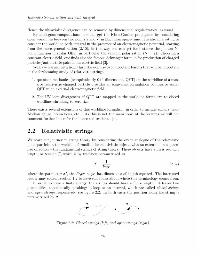
In order to have a finite energy, the strings should have a finite length. It leaves twopossibilities, topologically speaking: a loop or an interval, which are called closed stringsand open strings respectively, see figure 2.2. In both cases the position along the string isparametrized by σ.
σ σ
Figure 2.2: Closed strings (left) and open strings (right).
25

Bosonic strings: action and path integral
σ
τ
Figure 2.3: Closed string worldsheet.
Open strings are a little bit more subtle to handle, as one has to specify what are theboundary conditions at the end of the strings. We will deal mostly in these lectures withclosed strings.
Classical closed strings
A propagating relativistic closed string swaps in spacetime a two-dimensional surface s, orworldsheet, in analogy with the worldline of point particles. It has the topology of a cylinder,parametrized by σ for the space-like direction and τ for the time-like direction, see fig. 2.3.For closed strings, the coordinate σ is periodic. We choose the convention
σ ∼ σ+ 2π . (2.53)
The worldsheet swapped by a relativistic closed string in a space-time M of metric Gdefines an embedding map, given in a patch of the manifold M by
S1 × R → M (2.54)
(σ, τ) 7→ xµ(σ, τ) , xµ(σ+ 2π, τ) = xµ(σ, τ) , (2.55)
where the set of functions xµ(σ, τ), µ = 0, . . . , D−1 should be periodic in σ. For conveniencewe will use the notation (σ0, σ1) = (τ, σ). The codomain of the map, i.e. the space-time Mwhere the string leaves, is usually called the target space of the string.
The space-time metric Gµν(xρ) of the ambient space-time induces a metric h on the
world-sheet parametrized by σ and τ:
hij = Gµν∂xµ(σk)
∂σi∂xν(σk)
∂σj, (2.56)
such that the area element on the worldsheet is given by
dA =√− deth dσ0dσ1 . (2.57)
26
Bosonic strings: action and path integral
The negative sign in the square root takes into account that the tangent space of the surfacecan be split into a time-like and a space-like directions over every point.
In complete analogy with the relativistic particle case, see eq. (2.5), one postulates astring action of the form
Sng = −1
2πα ′
∫dσ0∫ 2π0
dσ1√
− det Gµν[xρ(σk)]∂xµ(σk)
∂σi∂xν(σk)
∂σj. (2.58)
This action is known as the Nambu-Goto action [5, 6]. It is invariant under diffeomorphismsof the worldsheet as it should:
σi 7→ σi(σj) (2.59a)
dσ0dσ1 7→ (det∂iσj)−1dσ0dσ1 (2.59b)
∂xµ
∂σi∂xν
∂σj7→ ∂xµ
∂σl∂xν
∂σm∂iσ
l∂jσm . (2.59c)
In Minkowski space-time (Gµν = ηµν) the action is also invariant under space-time Poincaretransformations xµ 7→ λµνx
ν + aµ.In the point particle case, there was a natural coupling to the electromagnetic potential,
i.e. to the one form A(xµ) = A(xµ)ρdxρ. There exists an analogous coupling allowed for the
string, but this time to a two-form potential B(xµ) = 12Bρσ(x
µ)dxµ ∧ dxν, which is called theKalb-Ramond potential [7]:5
Skr = −1
2πα ′
∫s
B = −1
4πα ′
∫s
Bρσ[xµ(τ)]
∂xµ
∂σi∂xν
∂σjdσi ∧ dσj
= −1
4πα ′
∫s
dσ0dσ1εijBρσ∂xµ
∂σi∂xν
∂σj. (2.60)
As its one-dimensional cousin, the Kalb-Ramond coupling is independent of the parametriza-tion of the worldsheet as it does not depend explicitly on the two-dimensional induced metrich. Furthermore, one can naturally associate to the coupling (2.60) a gauge invariance
Bµν dxµ ∧ dxν 7→ Bµν dxµ ∧ dxν + d(Λνdxν) = Bµν dxµdxν + ∂µΛν dxµ ∧ dxν , (2.61)
where the parameter of the gauge transformation is a one-form Λ = Λµdxµ. This transfor-
mation leaves invariant (2.60) up to boundary terms using Stokes’ theorem:∫s
B 7→ ∫s
B+
∫s
dΛ =
∫s
B+
∫∂s
Λ . (2.62)
5We use the two-dimensional epsilon symbol with non-zero components ε01 = −ε10 = 1. Note that(− detγ)−1/2εij is a two-index contravariant antisymmetric tensor.
27
Bosonic strings: action and path integral
Polyakov action
The non-linear Nambu-Goto action (2.58) is not a convenient starting point for quantizingthe theory. In analogy with the relativistic particle case, we will introduce an independentworldsheet metric γ and consider instead the action known as the Polyakov action [8]:
Sp = −1
4πα ′
∫s
d2σ√− detγγijGµν∂ix
µ(σk)∂jxν(σk) , (2.63)
where the non-dynamical field γij(σk) is determined by its equation of motion. The Polyakov
action can be understood as the minimal coupling of a two-dimensional metric to a setof scalar fields, hence is automatically invariant under diffeomorphisms of the worldsheetσi 7→ σi(σk).
The equations of motion for the scalar fields xµ(σi) are easy to determine. Under anarbitrary variation of the fields xµ 7→ xµ + δxµ the variation of the action is
δSp = −1
2πα ′
∫s
d2σ√
− detγγijGµν∂ixµ(σk)∂jδx
ν(σk)
=1
2πα ′
∫s
d2σ∂j
(√− detγγijGµν∂ix
µ(σk))δxν(σk)
+1
2πα ′
∫s
d2σ∂j(√
− detγγijGµν∂ixµ(σk)δxν(σk)
). (2.64)
While the third term is a total derivative, and therefore do not play any role on a closedworldsheet which has no boundaries, the second term gives a Laplace equation :
∇i(Gµν∇ixν(σk)
)= 0 . (2.65)
So, whenever the target space is a flat Minkowski space-time, one can choose Gµν to beconstant and the fields xµ(σk) are just free massless fields in two-dimensions.
Let us now prove that the equation of motion of the dynamical metric γ in the Polyakovaction (2.63) gives back the Nambu-Goto action (2.58). Under an infinitesimal variationγ 7→ γ+ δγ, one finds that at first order
δSp = −1
4πα ′
∫s
d2σ√
− detγ
[δ(√− detγ)√− detγ
γklhkl + δγijGµν∂ix
µ∂jxν
]. (2.66)
Given that γijγjk = δik one finds at first order that
γijδγjk + γjkδγij = 0 =⇒ δγjk = −γijγklδγil (2.67)
andδ(√− detγ)√− detγ
=1
2δ ln(− detγ) =
1
2γijδγij . (2.68)
We obtain then
δSp = −1
4πα ′
∫s
d2σ√
− detγ
[1
2γijγklhkl − γ
ikγjlhkl
]δγij . (2.69)
28

Bosonic strings: action and path integral
The vanishing of the first order variation leads therefore to
1
2γijγklhkl = γ
ikγjlhkl =⇒ hij =1
2γklhklγij . (2.70)
The determinant of this relation gives
deth =
(1
2γklhkl
)2detγ , (2.71)
from which we deduce that
Sp = −1
4πα ′
∫d2σ√− detγγijhij = −
1
4πα ′
∫d2σ√− deth
(1
2γklhkl
)−1
γklhkl
= −1
2πα ′
∫d2σ√− deth = Sng (2.72)
Hence, at least classically, the Nambu-Goto and the Polyakov actions give equivalent dynam-ics for the relativistic strings.
The Polyakov action (2.63) is certainly not the most general action on the string world-sheet that one can write. First, the coupling to the Kalb-Ramond field, eq. (2.63), is indepen-dent of the worldsheet metric hence takes the same form in the Nambu-Goto and Polyakovformalisms. Second, an acute reader may have wondered why, in the Polyakov action, we didnot include a ”cosmological constant” term
−1
4π
∫d2σ√
− detγΛ , (2.73)
that would be analogous to the mass term∫
dτ e(τ)m2 in the worldline action (2.10) for therelativistic particle. Such a term would imply that
1
2γijγklhkl +
1
2α ′Λγij = γikγjlhkl . (2.74)
Contracting this equation with γij gives
γklhkl + α′Λ = γklhkl (2.75)
which has no solutions unless Λ = 0. This is a peculiarity of string actions, which is notshared with actions of particles or higher-dimensional extended objects.6 We will understandshortly its significance.
There exists a last possible coupling of the relativistic string that has no analogue in theparticle case. From the two-dimensional worldsheet metric γ one can construct the Ricci
6Indeed for a p-dimensional extended object, p+ 1 being the dimension of its worldvolume, everything isthe same except the contraction with γij which gives p+1
2(γklhkl + α
′Λ) = γklhkl.
29

Bosonic strings: action and path integral
scalar R[γ], and write down a last term in the action of the Einstein-Hilbert type (after allwe are considering a dynamical worldsheet metric):
χ(s) =1
4π
∫d2σ√
− detγR[γ] . (2.76)
In short, one has traded the problem of quantizing gravity in four dimensions to the problemof quantizing gravity in two dimensions! Einstein gravity is two dimensions is much simpler,as first it has no propagating degrees of freedom because of diffeorphism invariance (standardcounting gives -1 degrees of freedom). The Einstein-Hilbert action is actually a topologicalinvariant of the two-dimensional manifold s, known as the Gauss-Bonnet term. In Euclideanspace it is equal to the Euler characteristic χ(s) of the two-dimensional worldsheet. If theworldsheet is an oriented surface without boundaries, it is given by
χ(s) = 2− 2g (2.77)
where g is the number of handles, or ”holes”, of the surface. For the sphere g = 0, the torusg = 1, etc... We will come back latter to the significance of these topologies.
There exists a generalization of the Einstein-Hilbert term that involves a coupling to ascalar field in space time Φ(xµ) and that is not topological:
Sd =1
4π
∫d2σ√− detγΦ[xµ(σi)]R[γ] . (2.78)
The field Φ(xµ), which plays an important role in string theory, is called the dilaton.To summarize this discussion, the general fundamental string action is given by the sum
of (2.63), (2.63) and (2.78), hence a (1+1)-dimensional quantum field theory on the worlsheetgiven by:
S = −1
4πα ′
∫s
d2σ(√
− detγγijGµν + εijBµν
)∂ix
µ∂jxν −
1
4π
∫d2σ√− detγΦ[xµ(σi)]R[γ]
(2.79)This action describes the propagation of a single relativistic string in a background specifiedby a metric G, a Kalb-Ramond field B and a dilaton Φ. The later two have no obviousinterpretation at this stage; note that in four dimensions the Kalb-Ramond field is actuallyequivalent to a real pseudo-scalar field as its field strength H = dB is Hodge-dual to thedifferential of a scalar field: ?H = da.
2.3 Symmetries
We now turn to the path integral quantization of the bosonic string. To start, one has topay attention to the symmetries of the theory, in particular to the gauge symmetries thatneed to be carefully taken care of, as in the example of the point particle that we have dealtwith in section 2.1. As there we will consider the path integral with an imaginary time
30
Bosonic strings: action and path integral
coordinate, i.e. we will consider an Euclidean worldsheet of coordinates (σ1, σ2) = (σ1,−iσ0)endowed with an Euclidean metric γ. However we will keep the signature of space-time tobe (−,+, · · · ,+).7
To simplify the discussion, consider the action of a string action with vanishing Kalb-Ramond field and constant dilaton field:
S =1
4πα ′
∫s
d2σ√
detγγijGµν∂ixµ∂jx
ν +Φ0
4π
∫s
d2σ√
detγR[γ] . (2.80)
The symmetries of the theory splits into worldsheet and target space symmetries. Wewill start by looking at the latter. One has first target-space symmetries of the action (2.80)corresponding to symmetries of space-time.
If the space-time is Minskowki space-time (gµν = ηµν) the action is invariant underPoincare transformations:
xµ 7→ Λµνxµ + aµ , Λ ∈ SO(1, d− 1) . (2.81)
These are global symmetries of the two-dimensional field theory.Under diffeomorphisms in space-time, i.e. infinitesimal field redefinitions δxµ = rµ[xρ],
the Polyakov action (2.63) keeps the same form if we perform the change of space-time metricδGµν = −2∇(µrν) at the same time.
2.3.1 Worldsheet symmetries
The string action (2.80), or its more general version (2.79), is by design invariant undercoordinate transformations, or diffeomorphims of the worldsheet,
σi 7→ σi(σk) , (2.82a)
γij 7→ γij =∂σk
∂σi∂σl
∂σjγk` , (2.82b)
being a theory of two-dimensional gravity minimally coupled to scalar fields xµ(σ).The Polyakov action has an extra local symmetry, which corresponds to Weyl transfor-
mations of the world-sheet metric, i.e. local scale transformations:
γij 7→ e2ω(σi)γij , (2.83)
where ω(σi) is an arbitrary differentiable function on the two-dimensional manifold s. Thisproperty comes from the scaling of the determinant of the metric in d dimensions
detγWeyl7→ e2dω detγ , (2.84)
which, specialized to two dimensions, implies that the action (2.63) invariant under Weyltransformations. The Kalb-Ramond coupling (2.60) is also by definition invariant beingindependent of the metric.
7As we will see the price to pay will be the appearance of negative norm states. The latter can befortunately removed by using the gauge symmetry of the theory.
31
Bosonic strings: action and path integral
The Ricci scalar transforms simply under a Weyl rescaling of the metric. We leave as anexercise to show that, in d dimensions,
γ 7→ e2ωγ (2.85a)
R[γ] 7→ e−2ω(R[γ] − 2(d− 1)∇2ω− 2(d− 2)(d− 1)∂aω∂
aω). (2.85b)
In two dimensions, this expression implies that√
detγR[γ] transforms as a total derivative,since
√detγ∇2ω = ∂i(
√detγ∇iω). One concludes that, at the classical level, the dilaton
action (2.78) is not invariant under Weyl transformations, unless Φ is a constant, in whichcase it was expected since the two-dimensional Einstein-Hilbert term (2.76) is topological. Wewill see later on that, in the quantum theory, the story is somewhat altered by the presenceof anomalies.
A careful reader would have noticed that the Weyl symmetry is not present in the originalNambu-Goto action (2.58). One can trace back its origin to the equation of motion for theworldsheet metric, eq. (2.70), which is invariant under Weyl transformations. This featureof the Polyakov action is not problematic. The Weyl symmetry is a gauge symmetry, hencedoes not really correspond to a symmetry but rather to a redundancy of our description ofthe theory. In the path integral quantization of the theory, this gauge symmetry will need tobe taken care of properly, as the diffeomorphism invariance.
Finally, we notice that the cosmological constant term (2.73) that we considered to includein the action is not Weyl invariant, which explains why this term is forbidden in the firstplace by the gauge symmetries of the problem.
2.3.2 Gauge choice
The Euclidean path integral of the fundamental string is defined by a functional integralover the fields xµ as well as over the two-dimensional metrics γ – i.e. over Euclidianworldsheet geometries – moded out by the volume of the gauge group of the theory, made oftwo-dimensional diffeomorphisms and Weyl transformations.
As we have done for the point particle, we will properly define this path integral bygauge-fixing and introducing the corresponding Faddeev-Popov determinant. To start with,one associates to each two-dimensional metric γ its gauge orbit, the set of its images γΞ
under gauge transformations Ξ = (Σ,Ω) composed of diffeomorphisms and Weyl rescalings:
Ξ :
σi 7→ Σi(σk)
γij 7→ exp(2Ω) × ∂σk
∂Σi∂σl
∂Σjγk`
(2.86)
To define properly the gauge-fixing condition, one has then to understand how to classify allmetrics over two-dimensional surfaces into equivalence classes under gauge transformations.
The coarser classification of compact two-dimensional surfaces is according to their topol-ogy. If we restrict ourselves to oriented surfaces without boundaries, their topology is com-pletely specified by the number of handles in the surface, which is called its genus g. Ex-plicitly, surfaces with g = 0 have the topology of a sphere, surfaces of genus g = 1 have thetopology of a torus, etc... As we have no reasons to restrict ourselves to a particular type of
32
Bosonic strings: action and path integral
g−2s g 0s g 2s
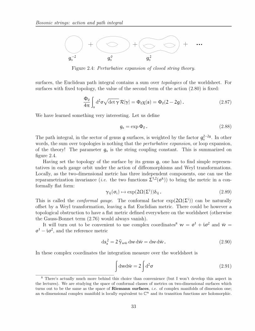
Figure 2.4: Perturbative expansion of closed string theory.
surfaces, the Euclidean path integral contains a sum over topologies of the worldsheet. Forsurfaces with fixed topology, the value of the second term of the action (2.80) is fixed:
Φ0
4π
∫s
d2σ√
detγR[γ] = Φ0χ(s) = Φ0(2− 2g) . (2.87)
We have learned something very interesting. Let us define
gs = expΦ0 . (2.88)
The path integral, in the sector of genus g surfaces, is weighted by the factor g2−2gs . In otherwords, the sum over topologies is nothing that the perturbative expansion, or loop expansion,of the theory! The parameter gs is the string coupling constant. This is summarized onfigure 2.4.
Having set the topology of the surface by its genus g, one has to find simple represen-tatives in each gauge orbit under the action of diffeomorphisms and Weyl transformations.Locally, as the two-dimensional metric has three independent components, one can use thereparametrization invariance (i.e. the two functions Σ1,2(σk)) to bring the metric in a con-formally flat form:
γij(σi) 7→ exp(2Ω(Σi))δij . (2.89)
This is called the conformal gauge. The conformal factor exp(2Ω(Σi)) can be naturallyoffset by a Weyl transformation, leaving a flat Euclidian metric. There could be however atopological obstruction to have a flat metric defined everywhere on the worldsheet (otherwisethe Gauss-Bonnet term (2.76) would always vanish).
It will turn out to be convenient to use complex coordinates8 w = σ1 + iσ2 and w =σ1 − iσ2, and the reference metric
ds 2s = 2 γww dw dw = dw dw . (2.90)
In these complex coordinates the integration measure over the worldsheet is∫dwdw = 2
∫d2σ (2.91)
8 There’s actually much more behind this choice than convenience (but I won’t develop this aspect inthe lectures). We are studying the space of conformal classes of metrics on two-dimensional surfaces whichturns out to be the same as the space of Riemann surfaces, i.e. of complex manifolds of dimension one;an n-dimensional complex manifold is locally equivalent to Cn and its transition functions are holomorphic.
33

Bosonic strings: action and path integral
and the holomorphic and anti-holomorphic derivatives:
∂ = ∂w = 12(∂1 − i∂2) , ∂ = ∂w = 1
2(∂1 + i∂2) . (2.92)
A generic infinitesimal gauge transformation (ı.e. an infinitesimal diffeomorphism togetherwith an infinitesimal Weyl transformation) around the flat metric is
δγij = 2δωδij − δjk∂iδσk − δik∂jδσ
k , (2.93)
which gives in complex coordinates
δγww = δω− 12(∂δw+ ∂δw) , (2.94a)
δγww = −∂δw , (2.94b)
δγww = −∂δw , (2.94c)
where δω, δw and δw are arbitrary differentiable functions of w and w.Finally, using complex coordinates, the Polyakov action (2.63) in the conformal gauge
takes the form
S =1
2πα ′
∫dwdw Gµν∂x
µ∂xν . (2.95)
This theory looks awfully simple in this gauge. Whenever the target space is flat, it seemsthat string theory reduces to a set of free scalar fields in two dimensions. However, one shouldnot forget that the equations of motion for the worldsheet metric γ should still be satisfied.By definition, the variation w.r.t. the metric of Polyakov action, which is just a theory oftwo-dimensional gravity coupled to some ”matter” fields xµ, is the stress energy tensor Tij,see chapter 3, eq. (3.17) for more details. Hence in the classical theory of strings we have toenforce the following constraint onto the solutions :
Tij = 0 . (2.96)
These constraints, which are known as Virasoro constraints, are the analogue of Gauss’ lawfor electromagnetism. Quantizing such constrained theory is a little bit subtle, and can bedone in particular using the BRST approach that we will develop in chapter 5.
2.3.3 Residual symmetries and moduli
In the study of the point particle path integral, we have seen two global aspects of theworldline geometry that played an important role: the existence of parameters, or moduli,that couldn’t be gauged away by the choice of reference metric and the existence of gaugetransformations that did not change the one-dimensional metric. In the string theory casethese two aspects are still relevant, and needs a little bit more effort to be understood.
The moduli are, by definition, given by changes of the metric that are orthogonal to gaugetransformations, i.e. that cannot be compensated for by a combination of a diffeomorphismand a Weyl transformation. In other words we consider a change of the metric δγij such that∫
d2σ(2δωδij − ∂iδjkδσ
k − ∂jδikδσk)δγij = 0 . (2.97)
34

Bosonic strings: action and path integral
This should hold true for any δω and δσk, hence it leads to a pair of independent relations:
Tr (δγ) = 0 =⇒ δγww = 0 (2.98a)
∂iδγij = 0 =⇒ ∂δγww = 0∂δγww = 0
(2.98b)
Solutions of these equations are called holomorphic quadratic differentials. The number ofindependent solutions will give the number of moduli of the surface nµ. In the mathematicalliterature, the space spanned by these moduli is called the Teichmuller space.
A second mismatch between the space of metric and the space of gauge transformationscorresponds to combinations of diffeomorphisms and Weyl transformations that leave themetric invariant. From equations (2.94b,2.94c) we learn that they correspond to diffeomor-phisms satisfying
∂δw = ∂δw = 0 , (2.99)
while the compensating Weyl transformation
δω = 12(∂δw+ ∂δw) (2.100)
is unambiguously determined by eq. (2.94a).The solutions of these equations are holomorphic vector fields, i.e. vectors fields that are
defined in any open set by a holomorphic function. The key point here is that we need to findvectors fields that satisfy globally this condition on the whole surface, which is a rather strongconstraint. These solutions are called the conformal Killing vectors (CKV) of the surface;the number of independent CKV will be called nk.
Figure 2.5: Mismatch between integrals over metrics and over the gauge group (diff+Weyl).
The number of moduli nµ and of conformal Killing vectors nk for a given surface arenot independent but related to each other by the Riemann-Roch theorem, in terms the Eulercharacteristic of the surface, which specifies its topology:
nµ − nk = −3χ(s) = 6(g− 1) . (2.101)
35
Bosonic strings: action and path integral
The sphere and the two-torus
We will now move away from this rather abstract discussion and derive in detail the moduliand conformal Killing vectors for the two most useful examples, the sphere and the torus.
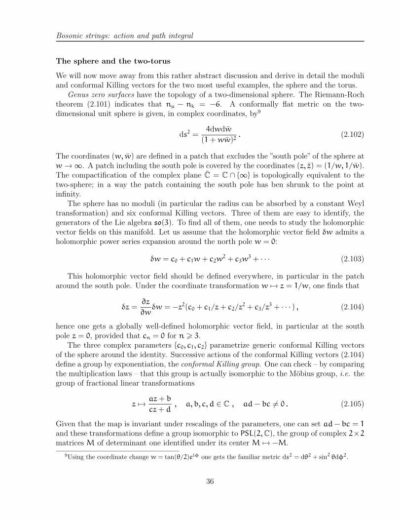
Genus zero surfaces have the topology of a two-dimensional sphere. The Riemann-Rochtheorem (2.101) indicates that nµ − nk = −6. A conformally flat metric on the two-dimensional unit sphere is given, in complex coordinates, by9
ds2 =4dwdw
(1+ww)2. (2.102)
The coordinates (w, w) are defined in a patch that excludes the ”south pole” of the sphere atw→∞. A patch including the south pole is covered by the coordinates (z, z) = (1/w, 1/w).The compactification of the complex plane C = C ∩ ∞ is topologically equivalent to thetwo-sphere; in a way the patch containing the south pole has ben shrunk to the point atinfinity.
The sphere has no moduli (in particular the radius can be absorbed by a constant Weyltransformation) and six conformal Killing vectors. Three of them are easy to identify, thegenerators of the Lie algebra so(3). To find all of them, one needs to study the holomorphicvector fields on this manifold. Let us assume that the holomorphic vector field δw admits aholomorphic power series expansion around the north pole w = 0:
δw = c0 + c1w+ c2w2 + c3w
3 + · · · (2.103)
This holomorphic vector field should be defined everywhere, in particular in the patcharound the south pole. Under the coordinate transformation w 7→ z = 1/w, one finds that
δz =∂z
∂wδw = −z2(c0 + c1/z+ c2/z
2 + c3/z3 + · · · ) , (2.104)
hence one gets a globally well-defined holomorphic vector field, in particular at the southpole z = 0, provided that cn = 0 for n > 3.
The three complex parameters c0, c1, c2 parametrize generic conformal Killing vectorsof the sphere around the identity. Successive actions of the conformal Killing vectors (2.104)define a group by exponentiation, the conformal Killing group. One can check – by comparingthe multiplication laws – that this group is actually isomorphic to the Mobius group, i.e. thegroup of fractional linear transformations
z 7→ az+ b
cz+ d, a, b, c, d ∈ C , ad− bc 6= 0 . (2.105)
Given that the map is invariant under rescalings of the parameters, one can set ad− bc = 1and these transformations define a group isomorphic to PSL(2,C), the group of complex 2×2matrices M of determinant one identified under its center M 7→ −M.
9Using the coordinate change w = tan(θ/2)eiφ one gets the familiar metric ds2 = dθ2 + sin2 θdφ2.
36

Bosonic strings: action and path integral
Genus one surfaces are topologically equivalent to a two-torus. The Euler characteristic ofthe two-torus vanishes, hence a two-torus can be endowed with a flat metric ds2 = dwdw. Thetorus has an obvious discrete Z2 symmetry w 7→ −w as well as two conformal Killing vectorscorresponding to translations along the two one-cycles of the torus. They are describedsimply by the constant holomorphic vector field δw = c0. According to the Riemann-Rochtheorem, one expects that the torus has two real moduli.
The torus can be described conveniently as the complex plane quotiented by the discreteidentifications
w ∼ w+ 2πnu1 + 2πmu2 , n,m ∈ Z , (2.106)
where u1 and u2 are complex parameters. By a rescaling of w, accompanied by a constantWeyl transformation, one can get rid of the former hence we consider the quotient
w ∼ w+ 2πn+ 2πmτ , n,m ∈ Z , (2.107)
where we have adopted the standard notation τ ∈ C for the torus modulus. As for the circularworldline in the point particle case, see the discussion above eqn. (2.16), an alternative wayto think about the torus is to consider the metric
ds2 = |dσ1 + τdσ2|2 , (2.108)
with the standard identifications σi ∼ σi + 2π. There exists some discrete ambiguity inthe identification of the parameter τ. First, the metric (2.108) is invariant under complexconjugation of the parameter τ, hence we can restrict the discussion to τ2 = =(τ) > 0 (thecase =(τ) = 0 being degenerate) i.e. to the upper half plane H. For a square torus, <(τ) = 0,while in general the real part of τ represents the way the circle parametrized by σ1 is ”twisted”before identifying the two enpoints of the cylinder.
The two-torus, being defined as a quotient of the complex plane, is nothing but a two-dimensional lattice, see fig. 2.6. It is obvious that the same lattice is described by replacing
Figure 2.6: Two-torus as a quotient of the complex plane.
τ by τ + 1. According to the metric (2.108) it amounts to redefine σ1 → σ1 + σ2, which iscompatible with the periodicities of the coordinates.
It it slightly less obvious to realize that another equivalent parametrization of the torusis given by τ 7→ −1/τ, if one allows a Weyl rescaling of the metric. Indeed starting from themetric (2.108) one gets∣∣dσ1 + τdσ2∣∣2 τ 7→−1/τ7−−−−−−→ ∣∣dσ1 − 1
τdσ2∣∣2 = 1
|τ|2
∣∣dσ2 − τdσ1∣∣2 . (2.109)
37
Bosonic strings: action and path integral
One sees that, up to a global rescaling of the metric, it amounts to replace σ1 → σ2 andσ2 → −σ1. In other words it exchanges the role of Euclidean worldsheet time and of thespace-like coordinate along the string. These two transformations generate the modular groupPSL(2,Z), which acts on the modular parameter as
τ 7→ aτ+ b
cτ+ d, a, b, c, d ∈ Z (2.110)
This group is indeed the group SL(2,Z) of 2× 2 integer matrices M of determinant one
M =
(a b
c d
), ad− bc = 1 , a, b, c, d ∈ Z (2.111)
quotiented by its center, i.e. with the identification M ∼ −M, as replacing (a, b, c, d) by(−a,−b,−c,−d) does not change the action (2.110). To avoid an over-counting in the pathintegral, we will choose to select a representative of the modular parameter τ into each orbitof the modular group. One can show that every point is the upper half plane H > 0 has aunique antecedent under the modular group in the fundamental domain F, defined by theconditions
F = τ ∈ H , |<(τ)| 6 12, |τ| > 1 , (2.112)
where the boundaries for <(τ) > 0 and <(τ) < 0 are identified, see fig. (2.7). In other words,the fundamental domain contains a unique point per orbit of PSL(2,Z).
1/2−1/2 1
F τ-plane
Figure 2.7: Fundamental domain F of the modular group.
To anticipate a little bit, this technical point will have drastic consequences. Rememberthat the torus diagram represents the one-loop contribution in the perturbative expansionin string theory, much as a circle represented the one-loop contribution in the point particlecase, see section 2.1. We have found there that the UV divergences in QFT were related
38

Bosonic strings: action and path integral
to circle of perimeter T going to zero size in the worldline formalism. In the string theorycase, it would correspond to the limit =(τ)→ 0, which is completely excluded from the pathintegral if we choose to integrate over F, the fundamental domain! This remarkable featureof string theory, which persists to higher order, indicates that the theory is UV-finite.
2.3.4 Conformal symmetry
Our discussion of conformal Killing vectors – i.e. of metric-preserving gauge symmetries –had been global as we only focused on holomorphic vector fields (2.99) defined everywhereon the manifold. This was important as we wanted to knew exactly the mismatch betweenintegrating over worldsheet metrics and over diffeomorphisms × Weyl gauge symmetries.There are however important properties of the quantum field theory defined on the worldsheetof the string by the gauge-fixed Polyakov action (2.95) that depend only on the symmetriesof the problem in an open set of the complex plane C.
If we allow the transformations (2.99) to be defined only in some patch of the worldsheet,they generate a much bigger group of symmetry. If we consider finite transformations ratherthan infinitesimal ones, what these equations tell us is that for any holomorphic function f,the change of coordinates
w 7→ f(w) (2.113a)
w 7→ f(w) (2.113b)
dw dw 7→ ∣∣∂wf(w)|−2dw dw (2.113c)
can be compensated by a Weyl transformation of parameter Ω = log |∂f| such as to leaveinvariant the flat two-dimensional metric.
This infinite-dimensional symmetry will play a crucial role in the following. The holo-morphic coordinate transformations (2.113a,2.113b) preserve the metric up to a local scaletransformation as can be seen from eqn. (2.113c), and the set of such transformations corre-sponds to the conformal group, which is indeed of infinite dimension precisely for a space ofdimension two.
We will obtain Ward identities associated with these symmetries for the two-dimensionalquantum field theory defined on the worldsheet, as such identities do not care about the well-definiteness of the symmetry at the global level. What we will obtain is an infinite numberof constraints on this QFT, which is every theoretical physicist dream!
2.4 Polyakov path integral
We have gathered the ingredients to define properly the path integral associated with thePolyakov action (2.95), which is a path integral over two-dimensional scalar fields xµ andover two-dimensional metrics γ on Euclidean worldsheets.
We have learned first in section 2.3 that the path integral splits into a sum over topologies,i.e. over surfaces of different genera g. In each sector we integrate over metrics γg of surfaces
39

Bosonic strings: action and path integral
with a given genus. Accordingly we are considering the formal vacuum amplitude
Z1 =
∞∑g=0
g2g−2s
∫Dγg
Vol(diff×Weyl)
∫Dx exp
(− Sp[γg, x]
), (2.114)
that receives contributions from single string worldsheets.As in the point particle case, we have formally divided the integral over the metrics
γg by the volume of the gauge group Vol(diff ×Weyl) in order to take care of the gaugeredundancies of the formulation of the theory. As there we will define properly this integralby the Faddeev-Popov method.
Inequivalent gauge orbits of metrics γg under diff×Weyl gauge transformations are labeledby a finite set of nµ parameters m`, the moduli. Along each of these orbits one can choose areference metric γg(m`), whose image under a transformation Ξ will be denoted γΞg (m`).
We want to trade the integral over the metrics γg by the product of an integral over themoduli and an integral over the gauge group, but the latter contains elements that do notchange the reference metric, the conformal Killing vectors. In the point particle case thisextra symmetry was taken care of by fixing the image of the origin under the diffeomorphismsof the worldline. In the present case we have to discuss separately the different topologies,as the outcome will be different. As before we will focus on the two most important cases,the sphere and the torus.
2.4.1 Path integral on the sphere
Surfaces of genus zero have positive curvature, see eqn. (2.76), and are all diff.×Weyl equiv-alent to the round unit two-sphere, as the latter has no moduli, see section 2.3.
The conformal Killing vectors on the two-sphere form a group isomorphic to PSL(2,C),the Mobius group, which is a non-compact Lie group of complex dimension three. One couldsplit the integral over diffeomorphisms as an integral over rotations and over diffeomorphismskeeping fixed the origin of the coordinates w = w = 0 (as we did for the point particle),taking care of the rotation subgroup SO(3) ⊂ PSL(2,C) but not of the full Mobius symmetry.
The vacuum amplitude path integral (2.114) contains the inverse of the volume of the Diff.× Weyl gauge group and therefore retains a factor of 1/Vol
(PSL(2,C)
)which vanishes, as
the Mobius group is non-compact. We learn that the vacuum amplitude on the sphere, i.e.at tree level, vanishes, as it should be because otherwise it would mean that we don’t expandaround a vacuum of the theory.10
Of course, string theory, as QFT, is not just about computing the vacuum amplitude.Physical observables correspond generically to time-ordered correlation functions of gauge-invariant observables of the theory. Because of diffeomorphism invariance, the observablestake the form
Ok =∫
d2w√
detγVk[xµ(w, w)] , (2.115)
10 As we will see below, the same conclusion can be obtained by noting that the zero-modes of the ghostpath integral measure will not be ”saturated” by the appropriate ghost insertions.
40

Bosonic strings: action and path integral
where Vk is some functional of the fields xµ(w, w) that transforms as a scalar under world-sheet diffeomorphisms; other constraints should be imposed on these functionals, and will bediscussed later. Then we have to consider path integrals of the form
〈O1 · · · On〉g=0 ∼ g−2s∫Dγ0Dx
n∏k=1
∫d2wk
√detγVke−Sp[x,γ0] . (2.116)
In this context the gauge-fixing problem that we had for the vacuum amplitude is easy tosolve. If the number n of operators is larger or equal to three, the Mobius symmetry iscompletely fixed by setting the positions (wk, wk) of three operators to arbitrary fixed values(wk, wk) instead of integrating over them.
To formulate the problem a bit differently, the integral∫Dγ0∏3
k=1 d2wk over the metricsand the position of three operators covers the whole gauge group, hence can be traded foran integral
∫DΞ which cancels out completely the volume of the gauge group in the path
integral (2.114).We define then the Faddeev-Popov determinant of string theory on the sphere in terms
of the path integral over the gauge group:11
1
∆fp(γ0):=
∫DΞ δ(γ0 − γ
Ξ0 )
3∏k=1
δ(wk − w
Ξk
)δ(wk − wΞk) (2.117)
where wk are arbitrary positions and wΞk their images under gauge transformations (diffeo-
morphisms of the surface). We obtain for the full path integral at tree-level
〈O1 · · · On〉g=0 = g−2s∫
Dγ0DΞ
Vol(diff×Weyl)∆fp(γ0)
n∏k=1
∫d2wk
√detγ0
∫Dx
n∏k=1
Vk[x(wk, wk)]
× exp(− Sp[γ0, x]
)δ(γ0 − γ
Ξ0 )
3∏k=1
δ (wk − wk)
= g−2s
∫Dx exp
(− Sp[ γ0, x]
)∆fp(γ0)
3∏k=1
√det γ0Vk[x(wk, wk)] n∏
k=4
OK . (2.118)
By diffeomorphisms and Weyl transformations, one can bring the metric on the sphere toa flat metric, the price to pay being that the south pole is mapped to |w|→∞. This is nota problem as long as we consider the compactification of the complex plane, C := C ∩∞,which is topologically a two-sphere.
In order to evaluate the Faddeev-Popov determinant, we first recall that the argument ofthe distribution δ(γ0 − γ
Ξ0 ) around the reference metric is given by eqns. (2.94). We have
11 Actually one should write ∆fp(γ0;wk, wk) as it depends also of the position of the fixed local operatorsbut we have chosen not to clutter the equations too much.
41
Bosonic strings: action and path integral
then
1
∆fp(γ0)=
∫DδωDδwDδw δ
[δω− 1
2(∂δw+ ∂δw)
]δ[∂δw
]δ[∂δw
]3∏k=1
δ(δw(wk, wk)) δ (δw(wk, wk)) . (2.119)
All these Dirac distributions are exponentiated by means of a corresponding Lagrange mul-tiplier:
1
∆fp(γ0)=
∫DδωDδwDδwDη Dβ Dβ
3∏k=1
dφkdφk
e2iπ∫
d2wη(δω−
12(∂δw+∂δw)
)e2iπ
∫d2wβ∂δwe2iπ
∫d2w β∂δwe2iπφkδw(wk,
wk)e2iπφkδw(wk, wk) (2.120)
We eventually need to insert the FP determinant rather than its inverse as for the particle,therefore we substitute for the variables (δω, δw, δw, η, β, β, φk, φk), the Grassmann vari-
ables (κ, c, c, ζ, b, b, ψk, ψk). We can compute immediately the integrals over κ, ζ, ψk andψk which gives, after a rescaling of the fields, the relatively simple expression:12
∆fp(γ0) =
∫DbDbDcDc e−
∫d2w2π
(b∂c+b∂c)
3∏k=1
c(wk)c( wk) (2.121)
To summarize the sphere path integral of string theory is given in its full glory by theexpression (n > 3):
〈O1 · · · On〉g=0 = g−2s∫DxDbDbDcDc e−
∫d2w2πα ′ gµν∂x
µ∂xνe−∫
d2w2π
(b∂c+b∂c)
3∏k=1
c(wk)c( wk)Vk[xµ(wk, wk)] n∏k=4
Ok , (2.122)
where wk are arbitrary positions, that we take usually to be 0, 1,+∞.
2.4.2 Path integral on the torus
The second important case is the two-torus, that corresponds to the one-loop amplitude instring theory, and present some differences with the previous case.
Gauge-inequivalent surfaces of genus one correspond to two-tori characterized by onecomplex parameter τ in the upper half-plane H = z ∈ C, =(z) > 0. Because of the ambiguity
12If we reinstall the index notation, we start with βij∂iδσj in the expansion of the Faddeev-Popov determi-
nant (2.117), which gives a ghost Lagrangian of the form bij∂icj, and in complex coordinates the components
are given below by eqn. (2.130).
42

Bosonic strings: action and path integral
in assigning a modular parameter τ to a given two-torus – or equivalently to a given two-dimensional lattice – one restricts further τ to be in the fundamental domain F of the modulargroup, see eqn. (2.112). A two-dimensional metric on the torus of complex modular parameter
τ = τ1 + iτ2 , |τ1| 6 12, τ 21 + τ
22 > 1 (2.123)
is then given by the flat metric (2.108) with σi ∼ σi + 2π.The two-torus has two real conformal Killing vectors, that are easy to understand, as they
correspond to translations along σ1 and along σ2. These translations form a group isomorphicto U(1)2, whose volume is 4π2τ2, the area of the torus of metric (2.108). It means that theintegral
∫d2τDΞ over the moduli and over the gauge group covers more that the integral∫
Dγ1 over the metrics on genus one surfaces.Fixing this extra symmetry is possible, even for the vacuum amplitude in the following
way (this is the same method that we used for the point particle vacuum amplitude). Ageneral diffeomorphism is given by two functions Σi(σk) that will not generically map theorigin of the coordinates σ1 = σ2 = 0 to the origin, as Σi(0, 0) 6= 0 in general. Because oftranslation invariance is possible to restrict the path integral to diffeomorphisms preservingthe origin, i.e. such that Σi(0, 0) = 0 or, say differently, for every diffeomorphism Σi one cantranslate back the image of the origin to Σi(0, 0) = 0, which will select an element of thetranslation group . In this way, the spurious gauge freedom will be removed. In addition tothese continuous symmetries, the torus metric is naturally invariant under the Z2 symmetryσi 7→ −σi, which doubles the volume of the group of metric-preserving gauge transformations.
These considerations lead to the following expression for the Faddeev-Popov determinanton the two-torus, as an integral over the gauge transformations Ξ = (Σ,Ω):
1
∆fp(γ1):=
∫F
d2τ
∫DΞ δ
(γ1 − γ
Ξ1 (τ)
)δ(Σ1(0)
)δ(Σ2(0)
), (2.124)
with the reference metric γ1(τ) obtained from eqn. (2.108)
γ1(τ) =
(1 τ1τ1 |τ|2
). (2.125)
Expanding the Dirac distribution near the reference metric gives
δ(γ1 − γ
Ξ1 (τ)
)=
δ(2δω− 2∂1(δσ
1 + τ1δσ2))δ(2|τ|2δω− 2∂2(|τ|
2δσ2 + τ1δσ1) + 2(τ1δτ1 + τ2δτ2)
)δ(2δωτ1 − ∂1(|τ|
2δσ2 + τ1δσ1) − ∂2(δσ
1 + τ1δσ2) + δτ1
)(2.126)
As before we introduce Lagrange multipliers fields. Compared to the sphere case as thereference metric is not diagonal it will be technically slightly more cumbersome. We introducea symmetric two-index tensor of Lagrange multipliers of components βij as well as a one-form
43

Bosonic strings: action and path integral
of components ηi. It gives
1
∆fp(γ1(τ))=
∫d2δτDδωDδσiDβijdηi exp
(2iπηiδσ
i(0))
exp 2iπτ2
∫d2σβ11(δω−∂1(δσ
1+τ1δσ2))+β22
(|τ|2δω−∂2(|τ|
2δσ2+τ1δσ1)+(τ1δτ1+τ2δτ2)
)+ β12
(2δωτ1 − ∂1(|τ|
2δσ2 + τ1δσ1) − ∂2(δσ
1 + τ1δσ2) + δτ1
)(2.127)
Integrating over δω imposes that the tensor β is traceless, i.e. that βijγ1(τ)ij = 0. Theremaining path integral in Dβ will be therefore on traceless tensors only. In order to get theFP determinant rather that its inverse, we replace (βij, δσi, ηi, δτ`) by Grassmann variables(bij, ci, ψi, κ`) and get after rescaling of the fields
∆fp(γ1(τ)) =
∫d2κDciDbijdψi exp
(ψic
i(0))
exp−1
2π
∫d2σ√
det γ1(τ) bij∂icj
× exp
12π
∫d2σ√
det γ1(τ)κ`bij∂τ`γ1(τ)ij
, (2.128)
which can be further simplified by integrating over κ` and over ψi.Inserting this result in the Polyakov path integral (2.114) one gets finally the vacuum
amplitude as13
Z1 =
∫F
dτdτ
16π2τ2
∫DxµDbijDci exp
−τ2
4π
∫d2σ
(bij∂icj +
1α ′gµνγ
ij1 ∂ix
µ∂jxν)
c1(0)c2(0) × τ2
4π
∫d2σbij∂τγ1(τ)ij ×
τ2
4π
∫d2σbij∂τγ1(τ)ij (2.129)
The dependence in 1/τ2 in the measure of integration over the modulus τ comes from thevolume of the group of translations along the torus, since have we have explained we don’tintegrate over this part of the gauge group. As we will see this factor ensures that the resultis invariant under the modular group PSL(2,Z).
It is finally convenient to come back to complex coordinates (w, w) = (σ1+τσ2, σ1+ τσ2).We write then
bww = b , bww = b , cw = c , cw = c (2.130)
The insertion in b(w, w) and b(w, w) takes in this basis the form
1
2πτ2
∫d2wb(w, w)
1
2πτ2
∫d2w b(w, w) , (2.131)
13The exact normalization of the result could be obtained by checking carefully how the insertions in thepath integral are normalized, however since the original path integral is ill-defined, and, since we did severalfield rescalings while manipulating formally the path integral, the honest way to get the factor right is to askthat the end result is properly normalized if interpreted as a partition function. Concretely if one chooses afully compact space-time one can request that the vacuum appears with degeneracy one.
44
Bosonic strings: action and path integral
As we will see later, one can replace b(w, w) by its value at any given point, for instancew = w = 0, as the non-zero modes of the field don’t contribute to the path integral (2.129).
Therefore we can replace∫
d2wb→ 4π2τ2b(0), and the same for the b insertion.We get the final result for the vacuum amplitude of string theory at one-loop as
Z1 =
∫F
d2τ
4τ2
∫DxµDbDbDcDc c(0)c(0)b(0)b(0)e−
∫d2w2π
(b∂c+b∂c+
1α ′gµν∂xµ∂xν
)(2.132)
The dependence of the integrand in the modulus τ is hidden in the periodicity of the complexvariable w ∼ w+ 1 ∼ w+ τ.
If one wants to compute a different observable as an n-point function 〈O1 · · · On〉g=1, itis enough to insert the operators Ok in the path integral above, as no gauge-fixing of theposition of some operators is needed in the present case.
This result is close to the sphere path integral (2.122), the differences reflecting the numberof moduli and conformal Killing vectors in each case. One can generalize of course thisdiscussion to surfaces of higher genera, but a rigorous presentation would be rather technical.
In this chapter we have assumed that the gauge symmetries of the classical theories,diffeomorphisms and Weyl transformations, were also valid in the quantum theory. As weshall see, the latter may be violated by an anomaly that put the theory in danger of beinginconsistent. Before proceeding to this computation, we will introduce in the next chapterthe powerful methods of two-dimensional conformal field theory.
2.5 Open strings
We will close this chapter with a very brief overview of open strings. Most of the mate-rial developed in the previous sections is relevant for open strings, however with some keymodifications.
First, the worldsheet of an open string is a strip rather than a cylinder, see fig. 2.8. Onehas therefore a map :
[0, π]× R → M (2.133)
(σ, τ) 7→ xµ(σ, τ) , (2.134)
where the set of functions xµ(σ, τ), µ = 0, . . . , D− 1 have some boundary conditions at theends of the interval, σ ∈ 0, π, that we will specify below.
Let us consider a classical open string in a generic curved space-time. It is governed bythe same Polyakov action as the bosonic string :
Sp = −1
4πα ′
∫s
d2σ√
− detγγijGµν∂ixµ∂jx
ν , (2.135)
If one considers the variation of the action w.r.t. the fields xµ, one picks in the present case
45
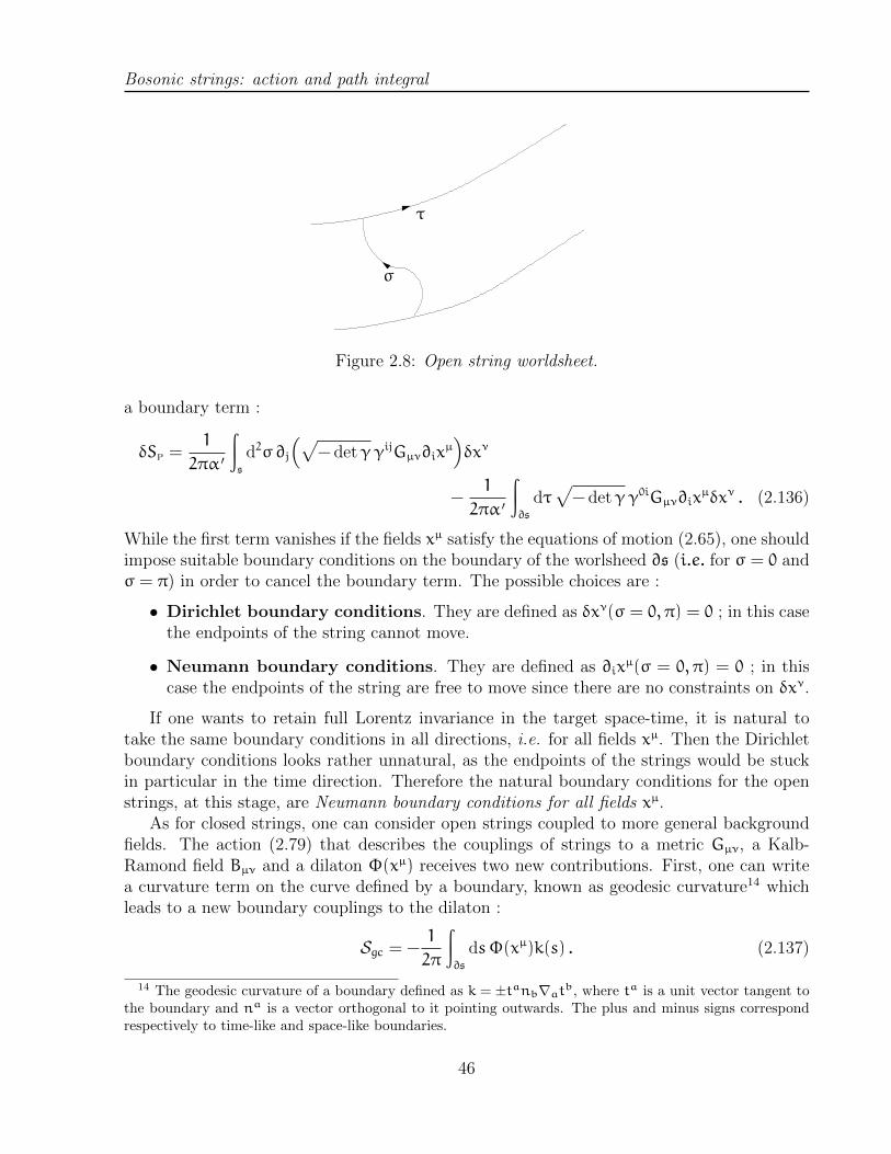
Bosonic strings: action and path integral
σ
τ
Figure 2.8: Open string worldsheet.
a boundary term :
δSp =1
2πα ′
∫s
d2σ∂j
(√− detγγijGµν∂ix
µ)δxν
−1
2πα ′
∫∂s
dτ√− detγγ0iGµν∂ix
µδxν . (2.136)
While the first term vanishes if the fields xµ satisfy the equations of motion (2.65), one shouldimpose suitable boundary conditions on the boundary of the worlsheed ∂s (i.e. for σ = 0 andσ = π) in order to cancel the boundary term. The possible choices are :
• Dirichlet boundary conditions. They are defined as δxν(σ = 0, π) = 0 ; in this casethe endpoints of the string cannot move.
• Neumann boundary conditions. They are defined as ∂ixµ(σ = 0, π) = 0 ; in this
case the endpoints of the string are free to move since there are no constraints on δxν.
If one wants to retain full Lorentz invariance in the target space-time, it is natural totake the same boundary conditions in all directions, i.e. for all fields xµ. Then the Dirichletboundary conditions looks rather unnatural, as the endpoints of the strings would be stuckin particular in the time direction. Therefore the natural boundary conditions for the openstrings, at this stage, are Neumann boundary conditions for all fields xµ.
As for closed strings, one can consider open strings coupled to more general backgroundfields. The action (2.79) that describes the couplings of strings to a metric Gµν, a Kalb-Ramond field Bµν and a dilaton Φ(xµ) receives two new contributions. First, one can writea curvature term on the curve defined by a boundary, known as geodesic curvature14 whichleads to a new boundary couplings to the dilaton :
Sgc = −1
2π
∫∂s
dsΦ(xµ)k(s) . (2.137)
14 The geodesic curvature of a boundary defined as k = ±tanb∇atb, where ta is a unit vector tangent tothe boundary and na is a vector orthogonal to it pointing outwards. The plus and minus signs correspondrespectively to time-like and space-like boundaries.
46

Bosonic strings: action and path integral
On an Eulidean world-sheet and with constant dilaton, this term and the other dilatoncoupling combine to the Euler characteristic of a surface with boundaries :
χ(s) =1
4π
∫d2σ√
detγR[γ] + 1
2π
∫∂s
ds k(s) . (2.138)
For a surface with g handles and b boundaries, the Euler characteristic is given by :
χ(s) = 2− 2g− b . (2.139)
Compared to the perturbative expansion of a theory of closed strings, see fig. 2.4, theperturbative expansion of a theory containing open strings receive new types of contributionscorresponding to surfaces with boundaries, see figure 2.9. Restricting as before to compactsurfaces, the first open string contributions are a disk (χ = 2 − 0 − 1 = 1) and a cylinder(χ = 2 − 0 − 2 = 0). As we will see, the disk is associated with tree-level contributions
g−1s g 0s
Figure 2.9: Perturbative expansion for open strings.
while the cylinder is associated with a one-loop contribution, if one considers the periodiccoordinate on the cylinder to be associated with Euclidean time on the worldsheet.
2.5.1 D-branes
D-branes appear quite naturally in string theory if one forgoes Lorentz invariance in the D-dimensional target space-time. One may impose only Lorentz invariance in p+ 1 space-timedimensions, in which case one can choose the following boundary conditions :
• Neumann boundary conditions for xµ, µ = 0, . . . , p
• Dirichlet boundary conditions for xM, M = p+ 1, . . . , D− 1.
Hence, at a given time, the endpoints of the open strings are attached to a space-like sub-manifold of dimension p. This sub-manifold, together with time, can be viewed as theworld-volume of a new extended object of string theory, known as a Dp-brane (where Dstands, of course, for Dirichlet).15 In the quantum theory this extended object is not rigid,
47

Bosonic strings: action and path integral
Figure 2.10: Open string with both ends on the same D-brane (blue) and ending on twodifferent D-branes (magenta).
but rather acquires dynamical properties. Open strings can have either both ends attachedto the same D-brane or each end of a different D-brane, see fig. 2.10.
On top of the boundary curvature coupling, see eqn. (2.137), another type of boundaryterm is allowed for the action of an open string. Let us consider for the moment that the openstring has Neumann boundary conditions along all space-like directions, i.e. that preservingLorentz invariance in D-dimensional space-time. Since each boundary of the string sweepsa worldline in space-time, it couples naturally to a one-form, i.e. to an Abelian gauge field,as the point-particle example studied in section 2.1. We supplement therefore the Polyakovaction of the string by the following contribution :
Sa =∫∂s
Aµdxµ . (2.140)
If the open string ends on a Dp-brane (with p < D− 1), it couples to an electromagneticfields in p + 1 dimensions. One can view this gauge field as living on the world-volume ofthe Dp-brane. If both ends of the string are on different D-branes, then each end couples toa different gauge field, each living on the corresponding worldvolume.16
Invariance of the coupling w.r.t. gauge transformations of the gauge fields is immediate,as in the point particle case. There is however another type of gauge invariance that weshould consider here. The variation of the Polyakov action under a gauge transformation ofthe Kalb-Ramond field Bµν was given, see eqn. (2.62), by∫
s
B 7→ ∫s
B+
∫∂s
Λµdxµ . (2.141)
On a worldsheet with boundaries, the second term is not zero, and should be canceled againstthe variation of the Abelian gauge field coupling 2.5.1. Therefore the general transformation
15 Whenever one chooses Neumann boundary conditions in all directions, one can consider that all spaceis filled by a D-brane.
16Whenever the positions of N Dp-branes coincide in all their transverse dimensions, the gauge symmetryU(1)N is actually enhanced to U(N) and the gauge theory becomes non-Abelian.
48

Bosonic strings: action and path integral
of the gauge field is
Aµ 7→ Aµ + ∂µλ−1
2πα ′Λµ , (2.142)
where the scalar λ is associated with the gauge symmetry of the Maxwell field Aµ and theone-form Λµdx
µ to the generalized gauge symmetry of the Kalb-Ramond field Bµν. Noticethat the field strength Fµν of the Maxwell field is not invariant under the latter. Rather, theinvariant combination under both gauge symmetries is
Fµν = Bµν + 2πα ′Fµν , (2.143)
which is therefore the natural object that should appear in low-energy effective actions forD-branes degrees of freedom.
2.5.2 Path integral
We end this section with a brief discussion about the path integral quantization of openstrings. The story is very similar to the case of closed strings, except that the number ofmoduli and conformal Killing vectors differ for the surfaces with boundaries under consider-ation. The Riemann-Roch theorem still holds, with now
nµ − nk = −3χ(s) = 3(2g+ b− 2) . (2.144)
The first surface under consideration is the disk, with g = 0 and b = 1 hence nµ−nk = −3.As the unit sphere, the disk has no moduli (since a change of radius can be absorbed by aWeyl rescaling). To obtain the conformal Killing vectors, one can obtain the unit disk fromthe unit sphere using the identification :
z ∼ 1/z . (2.145)
This identifies pairwise points inside and outside the unit disk in the complex plane, and theboundary of the disk |z| = 1 is left invariant. The conformal Killing vectors of the disk aretherefore obtained from those of the sphere that leave the boundary of the disk invariant. Itis rather straightforward to see that it consists of a subgroup of the Mobius group PSL(2,C),see eqn. (2.105), whose elements are of the form
z 7→ eiφz+ b
bz+ 1, |b| < 1 , φ ∈ R . (2.146)
It contains in particular rotations along the circle (b = 0). It is convenient to map the unitdisk to the upper half-plane using the conformal mapping
z 7→ w =z+ i
iz+ 1(2.147)
sending the boundary of the disk |z| = 1 to the real axis w ∈ R. In this case the relevantconformal Killing group is the subgroup of Mobius transformations leaving the real axisinvariant, i.e. the group PSL(2,R) :
w 7→ aw+ b
bw+ d, ad− bc = 1 , a, b, c, d ∈ R , (a, b, c, d) ∼ (−a,−b,−c,−d) . (2.148)
49

Bosonic strings: action and path integral
One can show, conjugating with the map (2.147), that the group of transformations (2.146)is isomorphic to PSL(2,R).
Since this group is non-compact, the situation is similar to what we have found for thesphere in the closed string sector. The vacuum amplitude vanishes, and the first non-vanishingobservable in the open string sector at tree-level is the correlation function of three boundaryoperators. There is another possibility however, with no direct analogue in the closed stringsector. One can consider a one-point function for an operator inside the disk, for instance atthe origin. Such configuration preserves only a compact subgroup U(1) of PSL(2,R) hencegives a non-zero answer. It represents the coupling between a closed string mode and aD-brane.
The cylinder has no holes and two boundaries and therefore, nµ−nk = 0. This surface hasa conformal Killing vector, corresponding to translations along the cylinder (i.e. in imaginarytime if one considers the open string channel), and a single real modulus, which can be takento be the length of the cylinder. One can therefore parametrize it as follows :
w = σ1 + iσ2 , σ1 ∈ [0, π] , σ2 ∼ σ2 + 2πt , t ∈ R>0 . (2.149)
One may wonder what would happen if we consider instead that the coordinate σ2 alongthe one-cycle of the cylinder is the space-like coordinate along a closed string and the co-ordinate σ1 along the interval is Euclidean time. While it does not make any difference inEuclidean signature, the interpretation is vastly different. Here we consider a process wherea closed string is emitted from the vacuum, propagates for some Euclidean time and is thenabsorbed. The fact that these two viewpoints are associated with the same field theoryquantity is known as channel duality between open and closed strings, see fig. 2.11. Thisobservation has far-reaching consequences ; in particular, it played a crucial role in the birthof the second string revolution, associated with the discovery of D-branes [9].
tt
Figure 2.11: Channel duality: open string channel (left panel) vs. closed string channel (rightpanel).
In the D-branes perspective channel duality has indeed the following meaning: the openstring viewpoint is interpreted as a one-loop vacuum amplitude for open strings whose end-points are attached to a pair of D-branes, while the closed string viewpoint is interpreted asthe tree-level emission of closed strings by the first D-brane, followed by their absorption bythe second D-brane.
50
Bosonic strings: action and path integral
References
[1] L. D. Faddeev and V. N. Popov, “Feynman Diagrams for the Yang-Mills Field,” Phys.Lett. 25B (1967) 29–30.
[2] C. Itzykson and J. B. Zuber, Quantum Field Theory. International Series In Pure andApplied Physics. McGraw-Hill, New York, 1980.
[3] J. S. Schwinger, “On gauge invariance and vacuum polarization,” Phys. Rev. 82 (1951)664–679.
[4] M. J. Strassler, “Field theory without Feynman diagrams: One loop effective actions,”Nucl. Phys. B385 (1992) 145–184, hep-ph/9205205.
[5] Y. Nambu, “Strings, Monopoles and Gauge Fields,” Phys. Rev. D10 (1974) 4262.
[6] T. Goto, “Relativistic quantum mechanics of one-dimensional mechanical continuum andsubsidiary condition of dual resonance model,” Prog. Theor. Phys. 46 (1971) 1560–1569.
[7] M. Kalb and P. Ramond, “Classical direct interstring action,” Phys. Rev. D9 (1974)2273–2284.
[8] A. M. Polyakov, “Quantum Geometry of Bosonic Strings,” Phys. Lett. 103B (1981) 207–210.
[9] J. Polchinski, “Dirichlet Branes and Ramond-Ramond charges,” Phys. Rev. Lett. 75(1995) 4724–4727, hep-th/9510017.
51

Chapter 3
Conformal field theory
52

Conformal symmetry
Two-dimensional conformally-invariant quantum field theories were introduced by Belavin,Polyakov, and Zamolodchikov in 1984 [1]. These theories play also an essential role in sta-tistical physics, for the description of critical phenomena in two dimensions. The book [2]is probably the most comprehensive book on the subject, and reference [3] is geared towardsstring applications.
After gauge-fixing of the diffeomorphisms and Weyl transformations to the flat worldsheetmetric ds2 = dwdw, the Euclidean Polyakov action
S =1
4πα ′
∫s
d2wGµν[Xρ]∂Xµ∂Xν (3.1)
has an infinite-dimensional residual gauge symmetry that consists in reparametrizations
w 7→ f(w) , w 7→ f(w) , (3.2)
where f is a holomorphic function, that leaves the metric invariant up to a conformal factor:
dwdw 7→ (∂f(w)
∂w
)(∂f(w)
∂w
)dwdw , (3.3)
and this conformal factor is absorbed by a Weyl transformation such that the reference metricdoes not change.
As we have seen previously, the topology of the worldsheet restricts severely the transfor-mations of this type that are allowed globally, i.e. the conformal Killing vectors of the surface.On the sphere we have found that they corresponded to the Mobius group PSL(2,C), whileon the two-torus the only holomorphic functions periodic around both of the one-cycles areconstants. As a result, the transformations (3.2) are not properly speaking local symmetriesof string theory itself. In addition we will see shortly that the Weyl symmetry might nothold in the quantum theory due to an anomaly.
At this stage we will be interested in a slightly different problem, the properties of two-dimensional quantum field theories defined on the complex plane1 (w, w), or on anothermanifold with a given fixed metric. We assume that the symmetries of the field theory in-cludes the geometrical transformations defined by eqn. (3.2). Quantum field theories withconformal invariance are called conformal field theories (CFTs for short). In two dimen-sions this symmetry is often powerful enough to solve exactly the theory, without using anyperturbative expansion.
It should be stressed that one considers a field theory on a two-dimensional manifoldwith a fixed metric, and the map w 7→ f(w), w 7→ f(w) is really changing the geometry, inparticular the distances between points. In a two-dimensional field theory coupled to gravity,this conformal map can be decomposed as a reparametrization (3.2) and a compensatingWeyl invariance.
The relation between two-dimensional CFTs and the Polyakov formulation of string theoryis as follows. When a conformal field theory in two-dimensions is coupled to two-dimensional
1 One often needs to consider the compactification of the complex plane by adding the point at infinity, C =C∩ ∞, which is related to the two-dimensional sphere (2.102) by a Weyl transformation ω = log(1+ww).
53

Conformal symmetry
gravity, it gives rise – at the classical level at least – to a Weyl-invariant theory. Conversely,after gauge-fixing of the diff.×Weyl local symmetry, the string theory action, which is nowformulated with respected to a fixed reference metric, is given in full generality by the actionof a two-dimensional conformal field theory.
3.1 The conformal group in diverse dimensions
The conformal group in two-dimensions is of infinite dimension, unlike the conformal groupin higher dimensions. To understand this we will study the conformal group in arbitraryEuclidean space-time of dimension D.
Conformal transformations are defined as coordinate transformations that preserve themetric up to a conformal factor, i.e.
xi 7→ xi(xj) , δijdxidxj 7→ δij
∂xi
∂xk∂xj
∂x`dxkdx` = exp
(2Ω(xk)
)δijdx
idxj . (3.4)
Here the metric is fixed, hence such transformation is really changing the geometry, in par-ticular distances between points. The defining propery of conformal transformations is topreserve angles between vectors of tangent space over any given point.
Let us consider a generic differentiable change of coordinates xi = xi + δxi(xj). At linearorder in δx, this change generates a conformal transformation of the D-dimensional metricγ provided that
∃α ∈ C0(RD) , −(∂`δxk + ∂kδx`) = α(xi)δk` . (3.5)
Taking the trace of tells us that −2∂iδxi = Dα, hence one has the equation
(∂`δxk + ∂kδx`) −2D(∂iδx
i)δk` = 0 . (3.6)
Acting on this equation with ∂` finally gives
δxk +(1− 2
D
)∂k(∂iδx
i) = 0 . (3.7)
Let us assume a power series expansion:
δxi = ai +mijxj + bix2 + xi(cjx
j) + O(x3) (3.8)
and look for constraints on all the coefficients. While a is unconstrainted, eqn. (3.6) tells usthat
m(ij) −1DδijTr (m) = 0 , (3.9)
hence m splits into a trace part and an antisymmetric part. Equation (3.7) becomes at thisorder
2Dbi + 2ci +(1− 2
D
)(2bi + (D+ 1)ci) = 0 (3.10)
which is solved for ci = −2bi.One can check that there are no solutions to the problem for higher order terms in (3.8)
if D > 2. The space of solutions of these equations is then finite and corresponds to:
54

Conformal symmetry
• translations: δxi = ai constant
• rotations: δxi = rijxj with r in the vector representation of so(D), i.e. the antisym-
metric part of m in eqn. (3.8)
• dilatations: δxi = λxi with λ a non-vanishing constant, i.e. the trace part of m ineqn. (3.8)
• special conformal transformations δxi = bi x2 − 2xi(bjxj) .
These are actually a set of generators of the Lie algebra so(D+ 1, 1), i.e. of the Lie Algebraof the Lorentz group in D+ 2 dimensions.
In two dimensions, the conformal transformations are given, in complex coordinates, byw 7→ f(w), w 7→ f(w) with f holomorphic, as we have already noticed. Naturally thisinfinite-dimensional group contains as a subgroup the transformations existing in generaldimensions. Explicitly:
• translations: δw = a, δw = a
• rotations: δw = iθw, δw = −iθw with θ ∈ R.
• dilatations: δw = λw, δw = λw with λ ∈ R.
• special conformal transformations δw = −b w2, δw = −b w2, b ∈ C.
Following the general discussion this generates a Lie group isomorphic to SO(3, 1), i.e. theLorentz group in three dimensions, whose component connected to the identity is isomorphicto the Mobius group PSL(2,C) that appeared already in section 2.3. It was shown there thatthe Mobius group was the subgroup of two-dimensional conformal transformations that areglobally defined on the two-sphere, or equivalently on the compactified complex plane C.
3.2 Radial quantization
The Euclidean two-dimensional conformal field theory associated with the worldsheet of apropagating string is naturally associated with a surface with the topology of a cylinder, i.e.parametrized by two coordinates (σ1, σ2) with σ1 ∼ σ1 + 2π, or equivalently the complexcoordinate w = σ1+ iσ2 with w ∼ w+ 2π. The coordinate σ2, which runs from −∞ to +∞,is the Euclidean time, obtain through Wick rotation: σ2 = −iτ.
Even outside the string theory context, the natural starting point for canonical quantiza-tion of conformal field theories is on the cylinder, in order to avoid infrared problems in thecase of an infinite space direction.
States of the quantum field theory are defined on a space-like slice, i.e. on a slice ofconstant σ2 after Wick rotation to Euclidean space. In particular, an initial state |in〉 of thetheory is defined on a slice with σ2 → −∞.
55

Conformal symmetry
Invariance of the theory under conformal transformation allows to give a different repre-sentation of the (Euclidean) time evolution of the QFT and of states of the theory. Let usconsider the conformal mapping from the cylinder to the complex plane:
w 7→ z = e−iw , w 7→ z = eiw . (3.11)
z-plane
Q =∮j0dz
|in〉
|in〉
radial time |z|
Q =∮j0dσ1
−∞
σ2
w-plane
Figure 3.1: Conformal mapping from the cylinder to the complex plane.
In this description, σ2 → −∞ is mapped to the origin z = 0 and slices of constant σ2 aremapped to circles around the origin, see fig. 3.1.
Time evolution correspond to dilatations or, said differently, the Hamiltonian operatorcorresponds to the dilatation operator. Likewise, time-ordered correlation functions of theQFT become radial-ordered correlation functions.
3.2.1 State - operator correspondence
In quantum field theories, states and operators are very different kind of objects.On the one hand, in the path integral formalism, a state corresponds to a wave functional
Ψ1[φ1(~x), t1] defined on a whole space-like slice of space-time at a given time t1, in the presentcase on the circle parametrized by σ. Such a state will evolve to an other state Ψ2[φ2(~x), t2]defined on a space-like slice at time t2 through:2
Ψ2[φ2(~x), t2] =
∫Dφ1Ψ1[φ1(~x, t1)]
∫φ(~x,t2)=φ2(~x)φ(~x,t1)=φ1(~x)
DφeiS[φ] . (3.12)
2A wave functional Ψ[φ(~x)] in QFT gives the probability amplitude associated with the whole field con-figuration φ(~x) on the space-like slice. In quantum mechanics, a state is defined by a wave-function ψ(q)
and the analoguous formula is ψ2(q2, t2) =∫
dq1 Ψ1(q1, t1)∫q(t2)=q2
q(t1)=q1Dq exp i
~∫t2t1
dt ′L.
56
Conformal symmetry
On the other hand, local operators in quantum field theories are defined as arbitrary localexpressions constructed from the elementary fields of the theory and their derivatives, i.e.local functionals O[φi, ∂νφ
i, · · · ](xµ).3The conformal mapping between the cylinder and the plane has some surprising conse-
quence. Let us consider an initial state |in〉 of the CFT on the cylinder, defined on the circleparametrized by σ1 in the infinite past σ2 → −∞. Under the conformal mapping (3.11) itis mapped to the origin of the plane z = z = 0. This means that the initial state is mappedto a local object at the origin, in other words a local operator, inserted at the origin. This iscalled the state-operator correspondence:
A|0〉 ←→ limz→0,z→0OA(z, z) , (3.13)
which says that a state obtained by acting on the vacuum with some operator A is equivalentto a local operator OA(z, z) inserted at the origin of the complex plane. In this perspectivethe vacuum |0〉 corresponds to the identity operator on the right-hand side.
3.2.2 Conserved charges
Let us consider a field theory with a conserved current, ∂µjµ = 0, and a certain space-like
foliation of the ambient space-time. One can define a conserved charge
Q =
∫jµdΣ
µ (3.14)
where dΣµ is the surface element over a space-like slice. For a conserved current on thecylindrical worldsheet of the string, it gives
Q =
∮j2
dσ1
2π. (3.15)
Let us map the theory to the plane. A two-dimensional current has components Jz(z, z)and Jz(z, z) in complex coordinates, and current conservation means that ∂Jz + ∂Jz = 0.
The integral around the cylinder∫
dσ1j2 becomes an integral over the polar angle,∫
dθ Jr.In complex coordinates, one obtains
Q =1
2iπ
(∮CJzdz−
∮CJzdz
), (3.16)
where C denotes a contour encircling the local operator corresponding to the state for whichwe compute the charge.
In many cases the two components of the current are separately conserved, hence J := Jz(z)is a holomorphic function and J := Jz(z) a anti-holomorphic one. This will be the case inparticular below for the charges associated respectively to holomorphic and anti-holomorphicconformal transformations.
3Note that, in a scalar field theory in 4d, a momentum state is given by |p〉 = a†(p)|0〉. However
a†(p) = −i∫
d3x eip·x↔∂0φ(x) is not a local operator, being integrated over a whole space-like slice.
57

Conformal symmetry
3.3 Conformal invariance and Ward identities
The dynamics of quantum field theories with conformal invariance is severely constrained bythis symmetry, especially in two dimensions where this symmetry is infinite dimensional.
3.3.1 Stress-energy tensor
In the classical theory, the stress-energy tensor obeys strong constraints for conformal invari-ance.
To derive the conservation laws associated with a general conformal field theory in D di-mensions, one considers the usual trick of coupling the field theory to a dynamical backgroundmetric γ. Then a coordinate change δσi(σk) accompanied by the change of background metricδγij = −∇iδσj −∇jδσi is a diffeomorphism, under which the theory should be invariant.
The transformation of the action under the infinitesimal change of the background metricis then opposite to the variation under the infinitesimal coordinate transformation δσi(σk)4:
δS = −1
2π
∫dDx δγij
δ
δγij
√− detγL =
1
4π
∫dDx
√− detγ T ijδγij
= −1
2π
∫dDx
√− detγ T ij∇iδσj (3.17)
where we have introduced the stress-energy tensor
T ij = −2√
− detγ
δ
δγij
√− detγL . (3.18)
Translation invariance of the theory implies then as usual that the stress-energy tensor iscovariantly conserved:
∇iTij = 0 . (3.19)
Let consider now invariance under scale transformations, which are special cases of con-formal transformations, corresponding to constant rescalings of the metric, δγij = δλγij.Equation (3.17) implies that the stress-energy tensor is traceless:
Tijγij = 0 . (3.20)
This is an essential property of conformal field theories.In two-dimensions, these expressions take a particularly simple form in complex coordi-
nates with a flat background metric:
∂Tz? + ∂Tz? = 0 (3.21)
for the former, andTzz = 0 (3.22)
4We work momentarily in Lorentzian signature for sake of comparison with the computation done in theGeneral relativity course.
58
Conformal symmetry
for the later. This means that the stress-energy tensor has only two non-vanishing compo-nents,
T := Tzz , T := Tzz , (3.23)
and that they are respectively holomorphic and anti-holomorphic functions:
∂Tzz = 0 =⇒ T = T(z) , (3.24a)
∂Tzz = 0 =⇒ T = T(z) . (3.24b)
We will finally give the form of the Noether currents associated with conformal transfor-mations. Let us consider the infinitesimal transformation
z 7→ z+ ρ(z, z)ε(z) , z 7→ z+ ρ(z, z)ε(z) , (3.25)
which reduces to a conformal transformation for constant ρ and ρ. According to eqn. (3.17)the variation of the action of the theory is then
δS = −1
2π
∫d2zT(z)∂
(ρ(z, z)ε(z)
)+ T(z)∂
(ρ(z, z)ε(z)
)= −
1
2π
∫d2z(T(z)ε(z)∂ρ(z, z) + T(z)ε(z)∂ρ(z, z)
)(3.26)
A very powerful point of view in two-dimensional Euclidean QFT is to consider w andw are independent variables. This means that we consider the analytic continuation of theEuclidean space R2 to C2, and the move from coordinates (σ1, σ2) to (w, w) just as a changeof basis in C2. Naturally at the end of the day one should enforce the reality condition(z)? = z.
From this point of view one can consider purely holomorphic conformal transformations,i.e. with ε = 0. The associated Noether current is then
Jz = T(z)ε(z) , Jz = 0 (3.27)
The non-zero component of the current, J := Jz is then holomorphic: ∂J = 0.In the same way a purely anti-holomorphic conformal transformation, , i.e. with ε = 0,
gives the conserved currentJz = 0 , Jz = T(z)ε(z) , (3.28)
whose non-zero component J := Jz is anti-holomorphic: ∂J = 0.As in other quantum field theories, these classical equations lead to functional equations
in the quantum theory, known as Ward identities that we shall study now.
59

Conformal symmetry
3.3.2 Ward identities
Let us consider a generic time-ordered N-point correlation function of local operators in atwo-dimensional conformal field theory. By local operator we mean any operator that canbe written as a local expression in the fundamental fields φi and their derivatives. Thecorresponding path integral is written as
〈O1(z1, z1) · · ·ON(zN, zN)〉 =1
Z
∫Dφie−S[φ
i]O1[φi](z1, z1) · · ·ON[φi](zN, zN) (3.29)
We consider a holomorphic conformal transformation with support in a small disc d in thecomplex plane, i.e. a transformation (3.25) with ρ non-vanishing only in the neighborhoodof some point (z0, z0) and ρ = 0.
There are two cases to consider: either there are no local operators in this neighborhood,or there is (at least) one inserted at a point inside the disk, see fig. 3.2.
(z1, z1)
(z1, z1)
(z2, z2)
(z3, z3) (z4, z4)
(z2, z2)
(z3, z3)
(z4, z4)
(z0, z0)
(z0, z0)
Figure 3.2: Conformal transformation with support away from local operators (left panel) andincluding one local operator (right panel).
Let us start with the former case. By construction the local operators are not affected bythe conformal transformation, hence the change in the path integral comes from the measureDφi and from the action S[φi] only. We will make the assumption that the measure isinvariant so the only variation comes from the action.5 The path integral is then modified atfirst order as∫
Dφie−S[φi]O1 · · ·ON 7→ ∫
Dφie−S[φi]
(1−
1
2π
∫d2z T(z)ε∂ρ
)O1 · · ·ON . (3.30)
The path integral should actually be completely independent of the transformation whichshould just be thought as some change of variables in the path integral. Therefore one gets
5This assumption is very strong and turns out actually to be wrong in many cases; this is the path integralview of QFT anomalies. We will come back to this important issue later on.
60

Conformal symmetry
the constraint, after integration by parts∫Dφie−S[φ
i]
∫d2z ρ(z, z) ∂
(T(z)ε(z)
)O1(z1, z1) · · ·ON(zN, zN) = 0 (3.31)
Since this should hold for any choice of ρ, we are led to the condition that6⟨∂(T(z)ε(z)
)O1(z1, z1) · · ·ON(zN, zN)
⟩= 0 . (3.32)
This is the quantum version of Noether theorem; naturally there is an analogous formula foranti-holomorphic conformal transformations.
We move now to the latter case. Let assume that the operator O(z1, z1) is inserted at apoint where ρ 6= 0, i.e. where the conformal transformation has support. Then on generalgrounds the operator transforms
O(z1, z1) 7→ O(z1, z1) + δO(z1, z1) . (3.33)
We insert this transformation in the path integral and, using similar arguments as before, weget at first order the relation
−1
2π
∫d2z ρ(z, z)
⟨∂(T(z)ε(z)
)O1(z1, z1) · · ·ON(zN, zN)
⟩=⟨δO1(z1, z1)O2(z2, z2) · · ·ON(zN, zN)
⟩. (3.34)
The function ρ being arbitrary, we can take it to be the indicator function of the disk daround (z0, z0). The left-hand side can then be simplified using Stokes’ theorem:∫
d
(∂zJ
z + ∂zJz)= −i
∮∂d
(Jzdz− Jzdz) . (3.35)
In the present case Jz = 0 as we found before so eqn. (3.34) gives
i
2π
∮∂d
dz⟨T(z)ε(z)O1(z1, z1)O2 · · ·ON
⟩=⟨δO1(z1, z1)O2 · · ·ON
⟩, (z1, z1) ∈ d . (3.36)
This teaches us a very important result: the change of an operator δO under a conformaltransformation is given by the residue of its product with the stress-energy tensor, namely
δO1(z1, z1) =i
2π
∮∂d
dz T(z)ε(z)O1(z1, z1) = −Resz→z1 (T(z)ε(z)O1(z1, z1)) (3.37)
The holomorphic function ε being arbitrary, this means that the operator product betweenT(z) and O(z1, z1) has a first order pole when they approach to each other:
T(z)O1(z1, z1) = · · ·+Res (T(z)O1(z1, z1))
z− z1+ · · · . (3.38)
6Naturally the same holds for the partition function Z in the denominator of (3.29), i.e. the zero-pointfunction.
61
Conformal symmetry
There is naturally a similar story for the anti-holomorphic conformal transformations, whichgives in particular:
T(z)O1(z1, z1) = · · ·+Res
(T(z)O1(z1, z1)
)z− z1
+ · · · . (3.39)
In a quantum field theory, product of operators make sense when they are time-ordered. Inthe context of radial quantization of a two-dimensional CFT, time-ordering takes the formof radial ordering, namely:
R (O1(z′, z ′)O2(z, z)) =
O1(z
′, z ′)O2(z, z) |z ′| > |z|
(−1)FO2(z, z)O1(z′, z ′) |z| > |z ′|
, (3.40)
where (−)F = 1 (resp. (−)F = −1) for bosonic (resp. fermionic) operators. In order tounclutter calculations, radial-ordering will always be implicit in operator equations like (3.38).
Singularities when operators approach each other such as (3.38) are a generic featureof quantum field theories. They have been studied more systematically under the nameof operator product expansions. The operator product expansion exists in all quantum fieldtheories, and provides the behavior of the theory when two operators O1 and O2 come close toeach other. The basic idea is that, when the separation between them become infinitesimal,one can expand the product into a sum of local operators. While this is usually an asymptoticexpansion only, one can show that in the case of conformal field theories the series converges,with the radius of convergence given by the distance to the nearest operator On6=1,2.
3.4 Primary operators
The variation of a generic local operator O(z, z) under a holomorphic conformal transforma-tion ε(z) is contained in eqn (3.37). We can get some insight by looking at specific simpletransformations.
Let us look first at a holomorphic translation defined as z 7→ z+a, z 7→ z. It acts on anylocal operator O as
O(z, z) 7→ O(z− a, z) = O(z, z) − a∂zO(z, z) + · · · (3.41)
By identifying both sides of (3.37) one learns that
∂zO(z, z) = Resz ′→z (T(z ′)O(z, z)) (3.42)
or in other words, after doing the same for anti-holomorphic translations:
T(z ′)O(z, z)z ′→z' · · ·+ ∂O(z, z)
z ′ − z+ · · · (3.43a)
T(z ′)O(z, z)z ′→z' · · ·+ ∂O(z, z)
z ′ − z+ · · · (3.43b)
62
Conformal symmetry
We look now at infinitesimal scaling transformations, which are by definition the (non-holomorphic) transformations z 7→ (1 + δλ)z, z 7→ (1 + δλ)z, with real δλ. We consideroperators that are eigenstates of the dilatation operator; the corresponding eigenvalue iscalled the scaling dimension ∆ of the operator:7
O 7→ λ−∆O (3.44)
The transformation of an operator O∆ of scaling dimension ∆ under an infinitesimal scaletransformation is given by:
δO∆ = −δλ(∆O∆(z, z) + z∂O∆ + z∂O∆
). (3.45)
We consider finally infinitesimal rotations in the complex plane, given by z 7→ (1 + iδθ)z,z 7→ (1−iδθ)z with real δθ. Consider again an operator which is an eigenstate of the rotationoperator; its eigenvalue is called the spin s of the operator. The transformation law is givenby:
δOs = −iδθ(sOs(z, z) + z∂Os − z∂Os
). (3.46)
In order to use the holomorphic/antiholomorphic splitting of conformal transformationsthat we have used throughout, it is convenient to combine scalings and rotations into thecomplex transformations
δz = (δλ+ iδθ)z =: δα z , δz = (δλ− iδθ)z =: δα z . (3.47)
Consider common eigenstates of the dilatation and rotation operators. The eigenvalues arecalled the conformal weights (h, h) of the state, and are related to the scaling dimension andspin through
∆ = h+ h , s = h− h . (3.48)
We obtain then from the transformations (3.45,3.47) the infinititesimal transformations:
δαOh,h = −δα(hOh,h(z, z) + z∂Oh,h
), (3.49a)
δαOh,h = −δα(hOh,h(z, z) + z∂Oh,h
). (3.49b)
Under a finite scaling transformation and rotation, the operator of conformal weights (h, h)transforms as
Oh,h 7→ λ−∆e−isθOh,h =(λeiθ
)−h (λe−iθ
)−hOh,h . (3.50)
The residue formula (3.37) will provide then the relation between the (anti)holomorphicscale transformation and the operator product with the stress-energy tensor. One has first
hOh,h(z, z) + z∂Oh,h(z, z) = Resz ′→z (z ′T(z ′)O(z, z))= Resz ′→z ((z ′ − z)T(z ′)O(z, z)) + zResz ′→z (T(z)O(z, z)) (3.51)
7At the classical level ∆ is the same as the dimension in units of inverse length coming from dimensionalanalysis. For instance, a free massless scalar field in dimension D has an action 1
4π
∫dDx (∂φ)2, hence φ has
dimension (length)2−D, in other words scaling dimension ∆ = D− 2.
63

Conformal symmetry
which gives, using also eqn. (3.42)
hOh,h(z, z) = Resz ′→z ((z ′ − z)T(z ′)O(z, z)) (3.52)
In summary, we have learned that the operator product expansion of one of the componentsof the stress-energy tensor with an operator of conformal weight (h, h) contains the terms
T(z ′)Oh,h(z, z)z ′→z' · · ·+ h
(z ′ − z)2Oh,h(z, z) +
1
(z ′ − z)∂Oh,h(z, z) + · · · (3.53a)
T(z ′)Oh,h(z, z)z ′→z' · · ·+ h
(z ′ − z)2Oh,h(z, z) +
1
(z ′ − z)∂Oh,h(z, z) + · · · (3.53b)
The operator product with a generic operator of weights (h, h) contains in principle moresingular terms in the Laurent series expansion in powers of (z−w).
Conformal primary operators
A distinguished class of local operators in a two-dimensional conformal field theory are op-erators for which the terms written in eqns. (3.53) exhaust all the possible singular terms inthe expansion, namely
T(z ′)Oh,h(z, z)z ′→z' h
(z ′ − z)2Oh,h(z, z) +
1
(z ′ − z)∂Oh,h(z, z) + regular (3.54a)
T(z ′)Oh,h(z, z)z ′→z' h
(z ′ − z)2Oh,h(z, z) +
1
(z ′ − z)∂Oh,h(z, z) + regular (3.54b)
These are called primary operators, or primaries for short. Given that the regular termsin the expansions do not contain essential information, we will often remove them from theexpressions of the operator product expansions.
Primary operators are interesting because they have particularly simple transformationlaws under a generic holomorphic conformal transformation δz = ε(z). Using once again theresidue formula (3.37) and the OPE (3.54a) for primary operators one finds that
δεO = −Resz ′→zε(z ′)
(h
(z ′ − z)2Oh,h(z, z) +
1
(z ′ − z)∂Oh,h(z, z) + regular
). (3.55)
The infinitesimal conformal transformation ε(z) is by definition holomorphic in the neigh-borhood of z and can be Taylor-expanded there:
ε(z ′) = ε(z) + (z ′ − z)∂ε(z) +O((z ′ − z)2
)(3.56)
Therefore transformation of a primary operator under an infinitesimal generic conformaltransformation is given by
δεO(z, z) = −ε(z)∂Oh,h(z, z) − h(∂ε(z)
)Oh,h(z, z) . (3.57)
64
Conformal symmetry
This transformation law can be generalized to a finite – rather than infinitesimal –transformation, namely w 7→ w = f(w), as well as to its anti-holomorphic counterpartz 7→ ˜z = f(z). One finds then:
O(z, z) 7→ O(z, ˜z)=
(∂f
∂z
)−h(∂f
∂z
)−h
O(z, z) . (3.58)
Correlation functions of primary operators
Conformal invariance severely constraints the form of correlation functions between primaryoperators. Let us start with the simplest case, the two-point function:
〈O1(z1, z1)O2(z2, z2)〉 , (3.59)
where O1 (resp. O2) is a conformal primary of weights (h1, h1) (resp. (h2, h2)). Under aconformal transformation z 7→ y(z), z 7→ y(z) one should have
〈O1(y1, y1)O2(y2, y2)〉 =1
Z
∫Dφie
−S[φi]O1(y1, y1)O2[y2, y2]
=1
Z
∫Dφie
−S[φi]O1(y1, y1)O2(y2, y2)
=
(∂y
∂z(z1)
)−h1(∂y
∂z(z1)
)−h1(∂y
∂z(z2)
)−h2(∂y
∂z(z2)
)−h2
〈O1(z1, z1)O2(z2, z2)〉 (3.60)
Invariance under holomorphic and anti-holomorphic translations implies first that
〈O1(z1, z1)O2(z2, z2)〉 = f(z1 − z2, z1 − z2) . (3.61)
Next we investigate invariance under holomorphic and anti-holomorphic scale transforma-tions. It leads to the functional identities
f(λ× (z1 − z2), z1 − z2
)= λ−h1−h2f
(z1 − z2, z1 − z2
), (3.62a)
f(z1 − z2, λ× (z1 − z2)
)= λ−h1−h2f
(z1 − z2, z1 − z2
). (3.62b)
hence f is homogeneous of degree −(h1 + h2) (resp. of degree −(h1 + h2)) in z1 − z2 (resp.in z1 − z2). In other words,
f(z1 − z2, z1 − z2) =C12
(z1 − z2)h1+h2(z1 − z2)h1+h2, (3.63)
where C12 is some constant. We now impose invariance under the transformation z 7→ −1/z,which is simpler to handle than the special conformal transformation z 7→ z/(1 − b z). Onegets
1
(−1/z1 + 1/z2)h1+h2
=(1/z21
)−h1 (1/z22
)−h2 1
(z1 − z2)h1+h2=⇒ (z1z2)
h1+h2 = z2h11 z2h22 ,
(3.64)
65

Conformal symmetry
with a similar equation for the anti-holomorphic transformations. Therefore the two-pointfunction can be non-zero only if h1 = h2 and h1 = h2:
〈φ1(z1, z1)φ2(z2, z2)〉 =C12
(z1 − z2)h1+h2(z1 − z2)h1+h2δh1,h2δh1,h2 . (3.65)
Up to a constant, the two-point function is then completely fixed by invariance under theglobal conformal group PSL(2,C).8 The set of constants Cij associated with the two-pointsfunctions of quasi-primary operators of the same conformal weights define a matrix that canmapped to the identity by choosing an appropriate basis in field space.
There exists a similar story regarding the three-point function of primary operators. In-variance under PSL(2,C) reduces the three-point function computation to a single unknowncoefficient:
〈φ1(z1, z1)φ2(z2, z2)φ3(z3, z3)〉 = C1231
(z1 − z2)h1+h2−h3(z2 − z3)h2+h3−h1(z1 − z3)h3+h1−h2
× 1
(z1 − z2)h1+h2−h3(z2 − z3)h2+h3−h1(z1 − z3)h3+h1−h2. (3.66)
3.5 The Virasoro Algebra
The operator product expansions (3.53) are valid for all local operators that are eigenstatesof the dilatation and rotation operators. By dimensional analysis, the stress-energy tensorTij given by the definition (3.17) has scaling dimension ∆ = 2 in two dimensions. Under arotation z 7→ z ′ = eiθz its non-vanishing components transform as Tzz 7→ Tz ′z ′ = e
−2iθTzz andTzz 7→ Tz ′z ′ = e
2iθTzz.This analysis shows that T = Tzz is an operator of conformal weights (h, h) = (2, 0) while
T = Tzz is an operator of conformal weights (h, h) = (0, 2), see eq. (3.48). However nothingindicates that these are primary operators. Let us consider then the OPEs
T(z ′)T(z)z ′→z' · · ·+ 2
(z ′ − z)2T(z) +
1
(z ′ − z)∂T(z) + reg. (3.67a)
T(z ′)T(z)z ′→z' · · ·+ 2
(z ′ − z)2T(z) +
1
(z ′ − z)∂T(z) + reg. (3.67b)
3.5.1 The central charge
The missing information in the OPEs (3.67) are the possible terms more singular than 1/(z−w)2 in the expansion. The only universal operators that should appear in any conformal fieldtheory are the components of the stress energy tensor and the identity operator which has
8Actually all is needed is that the operators transform as (3.58) under the action of PSL(2,C), which isa weaker statement than asking that this equation holds true for any holomorphic function. Such operatorsare called quasi-primary operators.
66

Conformal symmetry
naturally conformal dimensions (h, h) = (0, 0). On general grounds, one should allow termsproportional to the identity on the right-hand side of eqns. (3.17). By dimensional analysis,T being of dimension (2,0), this term should come with the power (z ′ − z)−4 in the operatorproduct expansion:9
T(z ′)T(z)z ′→z' c
2(z ′ − z)4+
2
(z ′ − z)2T(z) +
1
(z ′ − z)∂T(z) + reg. (3.68a)
T(z ′)T(z)z ′→z' c
2(z ′ − z)4+
2
(z ′ − z)2T(z, z) +
1
(z ′ − z)∂T(z) + reg. (3.68b)
These OPEs depend on two C-numbers c and c that are called the central charges of theconformal field theory, and encode the failure of the components of the stress-energy tensorto be conformal primaries. They play a central role in the study of conformal field theories,characterizing in particular the number of degrees of freedom.
From the operator product expansion (3.68) one deduces the transformation of T underan arbitrary infinitesimal holomorphic conformal transformation:
δεT(z) = −Resz ′→zε(z ′)
(c
2(z ′ − z)4+
2
(z ′ − z)2T(z) +
1
(z ′ − z)∂T(z) + reg.
)= −
c
12ε ′′′(z) − 2ε ′(z)T(z) − ε(z)∂T(z) , (3.69)
and similarly
δεT(z) = −c
12ε ′′′(z) − 2ε ′(z)T(z) − ε(z)∂T(z) , (3.70)
Notice that for infinitesimal dilatations, rotations and special conformal transformations theterms proportional to the central charges vanish.
For finite transformation z 7→ z = f(z) and z 7→ z = f(z) the components of the stress-tensor transforms as
T(z) 7→ T(z) =
(∂f(z)
∂z
)−2 (T(z) +
c
12f(z), z
), (3.71a)
T(z) 7→ T(z) = (∂f(z)
∂z
)−2(T(z) +
c
12f(z), z
), (3.71b)
where one defines the Schwarzian derivative
f(z), z =2f ′′′(z)f ′(z) − 3(f ′′(z))2
2(f ′(z))2, (3.72)
which is compatible with the composition of successive conformal transformations.
9More singular terms would come with operators of negative conformal weights; as we will see later thisis forbidden in unitary conformal field theories.
67

Conformal symmetry
3.5.2 The Virasoro Algebra
The information contained in the operator product expansions (3.68) can be recast in adifferent way that will turn out to be very useful, as it will allow to study the properties ofthe CFT using the tools of representation theory.
To start, the components of the stress tensor T and T are respectively holomorphic andanti-holomorphic functions on the complex plane, hence admit a Laurent series expansion:
T =∑n∈Z
Ln
zn+2, T =
∑n∈Z
Ln
zn+2. (3.73)
The coefficients of the expansion can be found by a contour integral
Ln =
∮C
dz
2iπzn+1 T(z) (3.74a)
Ln = −
∮C
dz
2iπzn+1 T(z) (3.74b)
where C is a contour encircling the origin counter-clockwise. The mode Ln corresponds tothe conserved charge associated with the conformal transformation δz = zn+1 following thediscussion in subsection 3.2.2. In particular, L0 + L0 is the dilatation generator, L0 − L0 therotation generator, while L−1 and L−1 generate holomorphic and anti-holomorphic translationsrespectively.
In the quantum conformal field theory on the plane, we will consider the commutator oftwo Laurent modes of the stress-energy tensor. In other words, for any state |φ〉 in the theorywe consider the quantity
[Lm, Ln]|φ〉 = LmLn|φ〉− LnLm|φ〉 . (3.75)
The first term corresponds to applying first Ln to |φ〉 and then Lm, while the second onecorresponds to applying first Lm to |φ〉 and then Ln.
Using the state-operator correspondence, the state |φ〉 is mapped to an local operatorO(z, z) that we can put at the origin. We have learned also in section 3.2 that the charge of astate w.r.t. a holomorphic current is computed by a contour integral around the correspondinglocal operator, see eqn. (3.16).
Let us consider the circular contours C of radius R and C ′ of radius R ′ > R, both aroundthe origin. We have
LmLnO(0, 0) =
∮C ′
dz12iπ
∮C
dz22iπ
zm+11 zn+12 T(z1) T(z2)O(0, 0) (3.76a)
LnLmO(0, 0) =
∮C ′
dz22iπ
∮C
dz12iπ
zm+11 zn+12 T(z1) T(z2)O(0, 0) (3.76b)
were the operator products are implicitely radial-ordered, as explained above. In the followingwe will remove the operator O which plays no role in this computation; it is understood thatthe operators are applied to any local operator in the CFT inserted at the origin.
68
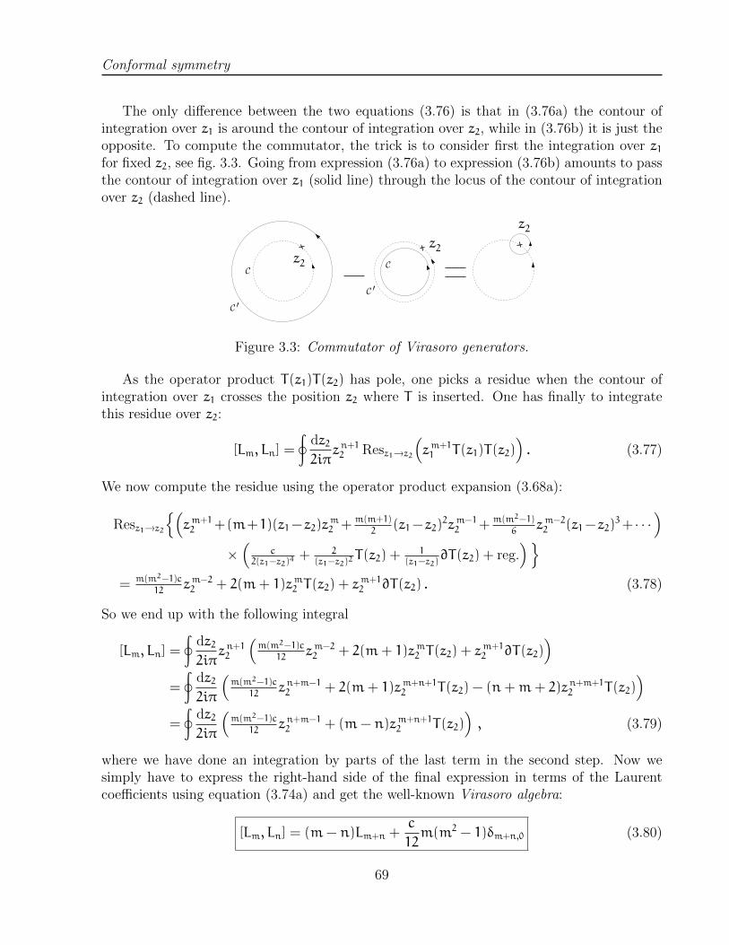
Conformal symmetry
The only difference between the two equations (3.76) is that in (3.76a) the contour ofintegration over z1 is around the contour of integration over z2, while in (3.76b) it is just theopposite. To compute the commutator, the trick is to consider first the integration over z1for fixed z2, see fig. 3.3. Going from expression (3.76a) to expression (3.76b) amounts to passthe contour of integration over z1 (solid line) through the locus of the contour of integrationover z2 (dashed line).
z2
z2
z2
C ′
C
C ′
C
Figure 3.3: Commutator of Virasoro generators.
As the operator product T(z1)T(z2) has pole, one picks a residue when the contour ofintegration over z1 crosses the position z2 where T is inserted. One has finally to integratethis residue over z2:
[Lm, Ln] =
∮dz22iπ
zn+12 Resz1→z2(zm+11 T(z1)T(z2)
). (3.77)
We now compute the residue using the operator product expansion (3.68a):
Resz1→z2(zm+12 +(m+1)(z1−z2)z
m2 + m(m+1)
2(z1−z2)
2zm−12 + m(m2−1)
6zm−22 (z1−z2)
3+ · · ·)
×(
c2(z1−z2)4
+ 2(z1−z2)2
T(z2) +1
(z1−z2)∂T(z2) + reg.
)= m(m2−1)c
12zm−22 + 2(m+ 1)zm2 T(z2) + z
m+12 ∂T(z2) . (3.78)
So we end up with the following integral
[Lm, Ln] =
∮dz22iπ
zn+12
(m(m2−1)c
12zm−22 + 2(m+ 1)zm2 T(z2) + z
m+12 ∂T(z2)
)=
∮dz22iπ
(m(m2−1)c
12zn+m−12 + 2(m+ 1)zm+n+1
2 T(z2) − (n+m+ 2)zn+m+12 T(z2)
)=
∮dz22iπ
(m(m2−1)c
12zn+m−12 + (m− n)zm+n+1
2 T(z2)), (3.79)
where we have done an integration by parts of the last term in the second step. Now wesimply have to express the right-hand side of the final expression in terms of the Laurentcoefficients using equation (3.74a) and get the well-known Virasoro algebra:
[Lm, Ln] = (m− n)Lm+n +c
12m(m2 − 1)δm+n,0 (3.80)
69

Conformal symmetry
If we did a similar computation, using the equation (3.74b) at the last step, we would findin the same way
[Lm, Ln] = (m− n)Lm+n +c
12m(m2 − 1)δm+n,0 . (3.81)
The Virasoro algebra (3.80) is very similar two an ordinary Lie algebra, except that it hasan infinite number of generators, Ln, n ∈ Z. Another characteristic feature is the presenceof the constant term c
12m(m2 − 1)δm+n,0, which commutes with all the generators; such a
term is called a central extension of the algebra.Finally a finite sub-algebra of the Virasoro algebra is obtained from the generators
L−1, L0, L1:[L0, L±1] = ∓L±1 , [L−1, L1] = 2L0 , (3.82)
which is isomorphic to sl(2,C); this is nothing but the Lie algebra of the Mobius group,the group of globally defined conformal transformations on the sphere C, i.e. of projectivetransformations z 7→ az+b
cz+d, a, b, c, d ∈ C, already discussed in subsection 2.3.3.
3.5.3 Conformally invariant vacuum and Casimir energy
When a conformal field theory theory is formulated on the cylinder, it is natural to expandthe components of the stress energy tensor in terms of its Fourier modes:
Tww = −∑n∈Z
Tneinw (3.83a)
Tww = −∑n∈Z
Tne−inw (3.83b)
with
Tn = −
∫dσ1
2πe−inσ1Tww(σ1, 0) , (3.84a)
Tn = −
∫dσ1
2πeinσ1Tww(σ1, 0) . (3.84b)
The conformal mapping (3.11) from the cylinder to the complex plane gives, using equa-tions (3.71) and (3.72):
Tww(w) = −z2Tzz(z) +c
24(3.85a)
Tww(w) = −z2Tzz(z) +c
24(3.85b)
Hence the expansion (3.73) on the plane in terms of Laurent coefficients and the expan-sion (3.83) on the cylinder in terms of Fourier modes are related through
Tn = Ln −c
24δn,0 , Tn = Ln −
c
24δn,0 . (3.86)
70

Conformal symmetry
In particular, the Hamiltonian of the conformal field theory on the cylinder is by definitionthe conserved charge associated with time translations:
H =
∫dσ1
2πTσ2σ2 = −
∫dσ1
2π
(Tww + Tww
)= L0 + L0 −
c+ c
24. (3.87)
Conformally invariant vacuum
In radial quantization, the natural vacuum state of the conformal field theory on the complexplane, |0〉, is defined by inserting the identity operator at the origin z = 0.
According to the definition (3.73) of the Virasoro generators, in order for the componentsof the stress-tensor to be non-singular at the origin, one should have
Ln|0〉 = 0 , Ln|0〉 = 0 , ∀n > −1 . (3.88)
In particular, the vacuum is invariant under the action of L−1, L0, L1 and L−1, L0, L1, i.e.under global conformal transformations. For this reason, it is called the PSL(2,C)-invariantvacuum.
If we consider a two-dimensional CFT in the PSL(2,C)-invariant vacuum on the plane,equation (3.87) indicates that the corresponding energy of the ground state on the cylinderis given by
Ecyl = −c+ c
24, (3.89)
which is interpreted as the Casimir energy of the QFT on the cylinder; notice that no regu-larization of high-energy divergences was needed to obtain this result. This remark providesanother interpretation of the central charges of a conformal field theory.
3.5.4 Conformal primaries revisited
Primary operators were defined by the operator product expansion (3.54) with the stress-energy tensor. Let us consider some primary operator Oh,h. Plugging in the decomposi-tions (3.73) in terms of Laurent modes, one finds that the corresponding state |O〉 is annihi-lated by all positive modes of the Virasoro generators:
∀n > 0 , Ln|h, h〉 = 0 , Ln|h, h〉 = 0 . (3.90)
Hence primary operators play the same role w.r.t. the Virasoro algebra as the highestweight vectors in representation theory of Lie algebras. For this reason they are also referredto as highest weight states of the Virasoro algebra.
The other states in the Virasoro representation associated with the highest weight state|h, h〉 are obtained by applying repeatedly the the negative Virasoro modes L−n, n > 0
(there is a similar story for anti-holomorphic generator). This generates what is known as aVerma module, that may or may not be an irreducible representation of the Virasoro algebradepending on the values of h and the central charge c.
71

Conformal symmetry
The conformal dimension of these descendant states, obtained from the highest weightstate using lowering operators L−n, is easily computed:
L0L−n|h, h〉 = nL−n|h, h〉+ L−nL0|h, h〉 = (h+ n)|h, h〉, n > 0 . (3.91)
I would certainly agree with the reader that would tell me that the primary states should becalled lowest dimension states rather than highest weight states!
3.5.5 Unitarity constraints
One important constraint on sensible quantum field theories is unitarity, the conservationof probabilities over time. The time evolution on the cylinder is given by the Hamiltoniandensity (with Minkowskian signature on the worldsheet):
H = −(Tww + Tww) =∑n∈Z
(Tne
in(σ1+τ) + Tne−in(σ1−τ)
)=∑n∈Z
(Lne
in(σ1+τ) + Lne−in(σ1−τ)
)−c+ c
24. (3.92)
Hence unitarity gives the constraints
(Ln)† = L−n ,
(Ln
)†= L−n . (3.93)
These unitarity relations have two immediate consequences:
• consider a primary state |h, h〉 of conformal dimensions (h, h) in a unitary CFT.
||L−1|h, h〉||2 = 〈h, h|[L1, L−1]|h, h〉 = 2〈h, h|L0|h, h〉 , (3.94)
hence in a unitary QFT the conformal dimensions (h, h) of primary operators – and,consequently, of all descendant states – should be non-negative. The unique statewith h = h = 0 in a unitary CFT is the PSL(2,C)-invariant vacuum since it satisfies
L−1|0, 0〉 = L−1|0, 0〉 = 0 which means in operator language ∂O0,0 = ∂O(0, 0) = 0.
• ∀n > 1, one has
||L−n|0〉||2 = 〈0|[Ln, L−n]|0〉 =c
12n(n2 − 1) , (3.95)
and similarly for Ln|h, h〉. Therefore a unitary CFT has positive central charges: c > 0and c > 0. The only unitary CFT with c = c = 0 is trivial and contains just theidentity operator.
72

Conformal symmetry
3.6 The Weyl anomaly
The failure of the components (T, T) of the stress-energy tensor to be primary operatorsw.r.t. generic two-dimensional conformal transformations is a just a characteristic feature ofconformal field theories, more precisely as we will see shortly of CFTs defined on a curved(two-dimensional) manifold. In the string theory context however, it leads to a potentialdisaster.
String theory was defined as a two-dimensional theory of gravity coupled to a set ofscalar matter fields xµ(σi). The theory has an enormous redundancy, since its gauge groupcorresponds to two-dimensional diffeomorphisms and Weyl transformations. After a suitablegauge-fixing procedure, we have obtained a path integral defined over a gauge slice, i.e. witha reference metric depending only on a handful of parameters. All this beautiful constructionfalls apart if the classical gauge symmetry of the theory is not satisfied at the quantum level.
The potential clash between gauge symmetry and quantum effects is associated with Weyltransformations. Heuristically it is not difficult to understand why. Computations in thetwo-dimensional quantum field theory we are dealing with have divergences, as in any otherQFT, that should be regularized. If one uses dimensional regularization, the invariance underWeyl rescalings is lost, since it depends crucially on being in dimension two, see eqn. (2.84).Using alternatively a Pauli-Villars regularization, one would introduce a scale in the theorybreaking explicitly scale invariance. As any sensible regulator breaks the Weyl symmetry, onemay wonder if at the end of the computation, which is not covariant w.r.t. the Weyl gaugetransformations, the invariance would be miraculously restored. It turns out not to be thecase and the Weyl symmetry has potentially an anomaly of the gauge symmetry signalingthe inconsistency of the theory.
To characterize this anomaly, one considers that the background geometry is fixed to somereference metric and consider whether the classical conservation laws associated with thesymmetries of the theory are truly independent of the choice of reference metric. Classically,Weyl-invariance implies that the stress-energy tensor is traceless, see eqn. (3.20). Because ofgeneral covariance of the theory, a quantum violation of this condition is very restricted. Inthe quantum field theory context, one would like to see whether the operator T ii inserted inan arbitrary correlation function gives zero. The more general parametrization is:
〈T ii · · · 〉 = aR[γ]〈· · · 〉 , (3.96)
where R[γ] is the Ricci scalar computed for the reference worldsheet metric γ, given that theright-hand side of the equation should be a local expression, and of scaling dimension two;the parameter a is dimensionless.
Since the diffeomorphism symmetry is not anomalous, one can work in the conformalgauge, ds2 = exp(2ω)dwdw, in which case, the anomaly equation becomes, using eqn. (2.85b),
2γww〈Tww · · · 〉 = −2ae−2ω∇2ω〈· · · 〉 =⇒ 〈Tww · · · 〉 = −a
2∇2ω〈· · · 〉 . (3.97)
The conservation of the stress-energy tensor gives ∇wTww + ∇wTww = 0. Hence taking the
73

Conformal symmetry
derivative of (3.97) with ∇w one reaches the equation:
〈∇wTww · · · 〉 =a
2∇w∇2ω〈· · · 〉 . (3.98)
Let us now consider an infinitesimal Weyl rescaling around the flat metric, i.e. ω = 1 +δω(w, w), and compare the variations of the left- and right-hand sides of eqn. (3.98).
In the previous section we have considered the transformation of the components of thestress-tensor of a two-dimensional CFT under an infinitesimal conformal transformation, i.e.an infinitesimal transformation w 7→ w+ ε(w):
− δT(w) =c
12∂3ε(w)︸ ︷︷ ︸Weyl
+ 2T(w)∂ε(w) + ε(w)∂T(w)︸ ︷︷ ︸tensor
, (3.99)
where the last two terms correspond to the standard tensorial transformation under a changeof coordinates, T ij(xk) 7→ T ij(xk) = (∂xi/∂xm)(∂xj/∂xn)Tmn(xk); the first term correspondsto the anomalous change of the operator T(w) under the compensating Weyl transformationthat brings back the metric to the original one.
Under the infinitesimal compensating Weyl transformation δω of the background metric,namely δω = 1
2(∂ε+∂ε) (see eq. 2.100), the stress-energy tensor operator transforms therefore
as:δδωT = −
c
6∂2wδω . (3.100)
Plugging into eqn. (3.98) one finds, using ∇w = 2∂w and ∇2 = 4∂w∂w,
−c
3∂w∂
2wδω = 4a∂2w∂wδω =⇒ a = −
c
12. (3.101)
The conclusion of this computation is that
〈T ii · · · 〉 = −c
12R[γ]〈· · · 〉 . (3.102)
This result is not problematic if one considers a conformal field theory outside of the stringtheory context, in the same way as the axial anomaly of quantum electrodynamics does notimply that the latter is an inconsistent quantum field theory.
However if the two-dimensional conformal field theory at hand corresponds to the world-sheet theory of a string the anomaly (3.102) indicates that the theory is inconsistent unlessc = 0. As we shall see this constraint will have far-reaching consequences.
A careful reader may have noticed that we could do exactly the same computation using∇wTww+∇wTww = 0, in which case we will reach the same equation as (3.102) with c replacedby c. These two equations are not consistent with each other unless c = c. It turns out that aconformal field theory with c 6= c cannot be coupled consistently to two-dimensional gravity;on top of the Weyl anomaly discussed here it has also a gravitational anomaly.
74
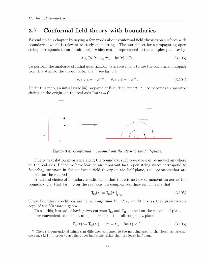
Conformal symmetry
3.7 Conformal field theory with boundaries
We end up this chapter by saying a few words about conformal field theories on surfaces withboundaries, which is relevant to study open strings. The worldsheet for a propagating openstring corresponds to an infinite strip, which can be represented in the complex plane w by
0 6 Re (w) 6 π , Im(z) ∈ R . (3.103)
To perform the analogue of radial quantization, is is convenient to use the conformal mappingfrom the strip to the upper half-plane10, see fig. 3.4:
w 7→ z = −e−iw , w 7→ z = −eiw . (3.104)
Under this map, an initial state |in〉 prepared at Euclidean time τ→ −∞ becomes an operatorsitting at the origin, on the real axis Im(z) = 0.
|in〉
−∞
σ2
z-plane
|in〉
radial time |z|
w-plane
Figure 3.4: Conformal mapping from the strip to the half-plane.
Due to translation invariance along the boundary, such operator can be moved anywhereon the real axis. Hence we have learned an important fact: open string states correspond toboundary operators in the conformal field theory on the half-plane, i.e. operators that aredefined on the real axis.
A natural choice of boundary conditions is that there is no flow of momentum across theboundary, i.e. that T01 = 0 on the real axis. In complex coordinates, it means that
Tzz(z) = Tzz(z)∣∣z=z. (3.105)
These boundary conditions are called conformal boundary conditions, as they preserve onecopy of the Virasoro algebra.
To see this, instead of having two currents Tzz and Tzz defined on the upper half-plane, isit more convenient to define a unique current on the full complex z plane :
Tzz(z) := Tzz(z′) , z ′ = z , Im(z) < 0 . (3.106)
10 There’s a conventional minus sign difference compared to the mapping used in the closed string case,see eqn. (3.11), in order to get the upper half-plane rather than the lower half-plane.
75

Conformal symmetry
The boundary condition (3.105) ensures naturally that Tzz is continuous across the boundary.Because of the boundary conditions, there exists a unique set of Virasoro generators. Let
us define C1/2 as a half-circular contour in the upper half-plane around the origin, and C0 aclosed circular contour around the oriign. The Virasoro generators are defined as :
Ln =1
2iπ
∫C1/2
(dz zn+1Tzz(z) − dz zn+1Tzz(z)
)=
1
2iπ
∮C0
dz zn+1Tzz(z) , (3.107)
where we have used the definition (3.106) in the second equality. The OPE between Tzzand itself is unchanged, since it is a local property of the field theory. Hence we get thesame Virasoro algebra (3.80) that we have obtained in the case of a CFT without boundary,however we have a single copy instead of two.
Another way to understand this is the following. The Virasoro generator Ln (resp. Ln) wasthe conserved charge associated to the holomorphic change of coordinates δz = ε(z) = zn+1
(resp. δz = ε(z) = zn+1). In the present context one should allow only transformations thatpreserve the boundary, i.e. the real axis. They should obey ε(z) = ε(z)|z=z.
The highest weight representations |h〉b of this Virasoro algebra correspond, under thestate-operator correspondence, to boundary primary operators Ob(x) defined on the real axis.
References
[1] A. A. Belavin, A. M. Polyakov, and A. B. Zamolodchikov, “Infinite Conformal Symmetryin Two-Dimensional Quantum Field Theory,” Nucl. Phys. B241 (1984) 333–380.
[2] P. Di Francesco, P. Mathieu, and D. Senechal, Conformal Field Theory. Graduate Textsin Contemporary Physics. Springer-Verlag, New York, 1997.
[3] R. Blumenhagen and E. Plauschinn, “Introduction to conformal field theory,” Lect. NotesPhys. 779 (2009) 1–256.
76

Chapter 4
Free conformal field theories
77

Free conformal field theories
The presentation of conformal field theories in two dimensions in chapter 3 was ratherformal and abstract. We will look at simple examples of conformal field theories, as freemassless scalar fields, that will eventually be the building blocks of bosonic string theory andlater on of the superstring theories.
4.1 Free scalar fields
The basic ingredients of the Polyakov action (3.1) in conformal gauge and with a flatMinkowski-space time target space are a set of scalar fields xµ(σi), µ ∈ 0, 1, . . . ,D − 1,governed by the free quadratic action:
S =1
4πα ′
∫d2σηµν δij ∂
ixµ∂jxν . (4.1)
Let us consider a single space-like coordinate, i.e. a free two-dimensional massless scalarfield with action
S =1
4πα ′
∫d2σ δij ∂
ix∂jx . (4.2)
The stress-energy tensor deduced from this action is given, following eqn. (3.17), by theexpression:
Tij =1
α ′∂ix∂jx−
1
2α ′δij∂kx∂
kx , (4.3)
In complex coordinates, the action becomes:
S =1
2πα ′
∫d2w∂x∂x , (4.4)
From now on we will consider the conformal field theory on the complex plane. Thenon-vanishing components of the stress tensor are
T(z) = −1
α ′∂x∂x , (4.5a)
T(z) = −1
α ′∂x∂x , (4.5b)
with Tzz = 0 because of two-dimensional conformal invariance of the action as stressed in theprevious chapter. The equations of motion following from (4.4) are simply
∂∂x(z, z) = 0 , (4.6)
hence x is the sum of a holomorphic and a anti-holomorphic function:1
x(z, z) = xL(z) + xR(z) (4.7)
1Whenever the target-space coordinate corresponding to the field x(z, z) is non-compact, the (anti-) holo-morphic functions xl(z) and xr(z) do not define by themselves consistent fields, are they are not univaluedon the plane, see eq. (4.31) below.
78

Free conformal field theories
On the Minkwoskian cylinder, i.e. with z = e−i(τ+σ) and z = e−i(τ−σ), the first term describesleft-moving waves and the second term right-moving ones. For this reason, the Virasoroalgebras corresponding to holomorphic and anti-holomorphic conformal transformations arecalled respectively left-moving and right-moving algebras.
The free scalar action (4.4) has a global symmetry on top of conformal symmetry, theinvariance under translations in target space:
x 7→ x+ a . (4.8)
From Noether theorem, and using the equation of motion (4.6), one finds conserved holomor-phic and anti-holomorphic currents:
J(z) := Jz(z) =1
α ′∂x , ∂J = 0 (4.9a)
J(z) := Jz(z) =1
α ′∂x , ∂J = 0 (4.9b)
Invariance of the action (4.4) under conformal transformations indicates that xµ has conformal
weights (0, 0), hence J (resp. J) has conformal weights (1, 0) (resp. conformal weights (0, 1)).One can apply the residue formula (3.37), that was established for conformal transforma-
tion but holds for any (anti)holomorphic conserved current in a two-dimensional CFT, if onesplits the translation of x into a translation of xL(z) by a/2 and a translation of xR(z) bya/2. It leads to the relation:
a/2 = δxL = −Resz ′→z (aJ(z ′)x(z, z))=⇒ a
1
α ′∂x(z ′)x(z, z) = · · ·− a
2(z ′ − z)+ regular. (4.10)
which implies that, using the same reasoning for the anti-holomorphic current
∂x(z ′)x(z, z) = −α ′
2(z ′ − z)+ reg. (4.11a)
∂x(z ′)x(z, z) = −α ′
2(z ′ − z)+ reg. (4.11b)
Because x has scaling dimensions (0, 0), and ∂x (resp. ∂x) has scaling dimension (1, 0) (resp.(0, 1)) it is actually impossible to get terms more singular than 1/(z ′ − z), as they would bemultiplied by operators of negative weights, which are forbidden in unitary conformal fieldtheories. Differenciating once with respect to z one gets the OPE between the currents
J(z ′)J(z) = −1
2α ′(z ′ − z)2+ reg. (4.12a)
J(z ′)J(z) = −1
2α ′(z ′ − z)2+ reg. (4.12b)
79

Free conformal field theories
Finally, integrating equations (4.11) w.r.t. z and z, one finds that the OPE between x(z, z)and itself is given by
x(z ′, z ′)x(z, z) = −α ′
2log(µ2(z− z ′)(z− z ′)
)+ reg. (4.13)
where the parameter µ is an infrared cut-off which is here for dimensional reasons. Thesingular term on the right-hand side of this equation is actually the (perhaps familiar) positionspace scalar Green function in two dimensions, that will be computed directly later on, seeeqn. (6.9). The present derivation was putting an emphasis on the symmetries of the theory.Unlike Green functions in higher dimensions, this one does not fall off at large distances,which eventually implies the absence of phase transitions for continuous symmetries in twodimensions.
4.1.1 Stress-energy tensor
The classical expressions (4.5) of the components of the stress-energy tensor should actuallybe regularized in the quantum theory.
Normal-ordered product
We define first the normal-ordered product of operators by subtracting the short-distancessingularities when the two operators approach each other:
••O1(z
′)O2(z)•• := O1(z
′)O2(z) − O1(z′)O2(z) , (4.14)
where O1(z′)O1(z) means all terms involving negative powers of (z ′− z) in the OPE between
O1 and O2. The relation between this normal ordering and the usual one (annihilationoperators to the right) will become more transparent later on. Note that eq. (4.14) is anoperator equation that should hold inserted in any correlation function; as such, the firstterm on the right-hand side should be understood as a time-ordered product (or rather inthe present context as a radial-ordered product).
When O1 and O2 are at coincident points we define the normal order product as a limit,namely:
••O1O2
•• (z) = lim
z ′→z(O1(z
′)O2(z) − O1(z′)O1(z)
)(4.15)
A convenient way of rewriting this expression uses a contour integral:
••O1O2
•• (z) =
1
2iπ
∫Cz
dz ′
z ′ − zO1(z
′)O2(z) , (4.16)
where Cz is a contour around z. The integral picks only the regular terms in the OPE of O1and O2 by construction.
80
Free conformal field theories
Finally we will consider in several computations the OPE between normal-ordered op-erators. One has the following generalization of Wick theorem to arbitrary interacting two-dimensional CFTs:
O1(z1)••O2O3
•• (z3) =
1
2iπ
∫Cz3
dz2z2 − z3
(O1(z1)O2(z2)O3(z3) + O2(z2)O1(z1)O3(z3)
)(4.17)
It can be applied iteratively to deal with more complicated operator products.
4.1.2 OPE of the stress-energy tensor
In terms of the normal product, applied to the bilinear of the current J of self-OPE (4.12),the quantum expression of T(z) reads:
T(z) = −α ′ •• JJ•• (z) , (4.18a)
T(z) = −α ′ •• JJ•• (z) , (4.18b)
with here:
•• JJ
•• (z) = lim
z ′→z(J(z ′)J(z) − J(z ′)J(z)
)= lim
z ′→z(J(z ′)J(z) +
α ′
2(z ′ − z)2
). (4.19)
In terms of the fundamental field x and its derivatives the stress energy tensor takes theform:
T(z) = −1
α ′•• ∂x∂x
•• (z) , (4.20a)
T(z) = −1
α ′•• ∂x∂x
•• (z) . (4.20b)
Using this definitions (4.20) we will now show that J and J are conformal primary opera-tors. One needs to compute the OPE:
T(z ′)J(z) = −1
(α ′)2•• ∂x∂x
•• (z
′)∂x(z) (4.21)
The OPE between the composite operator T and J is computed using (4.17). In the presentcase the computation is rather simple as the self-contraction of J gives just the identityoperator. Explicitly we have
T(z ′)J(z) = −1
(α ′)2•• ∂x∂x
•• (z
′)∂x(z)
= −1
(α ′)2∂x(z ′)∂x(z ′)∂x(z) −
1
(α ′)2∂x(z ′)∂x(z ′)∂x(z)
= −2
(α ′)2
(−
α ′
2(z ′ − z)2
)∂x(z ′)
=J(z)
(z ′ − z)2+
∂J(z)
(z ′ − z), (4.22)
81

Free conformal field theories
where we have used a Taylor expansion of the current J(z ′) around z in the last step,
J(z ′) = J(z) + (z ′ − z)∂J(z) +O((z ′ − z)2
)(4.23)
In order to determine the central charge of the free scalar conformal field theory, oneneeds to compute the OPE satisfied by T and T , using the OPE (4.13) of the elementary fieldand the definitions (4.20). One has to use the Wick contractions:
1
(α ′)2T(z ′)T(z) = •
• JJ•• (z
′) •• JJ•• (z) =
•• J(z
′)J(z ′)J(z)J(z) ••
+ •• J(z
′)J(z ′)J(z)J(z) •• +•• J(z
′)J(z ′)J(z)J(z) •• +•• J(z
′)J(z ′)J(z)J(z) ••
+ J(z ′)J(z ′)J(z)J(z) + J(z ′)J(z ′)J(z)J(z) (4.24)
which gives, using at the last step the Taylor expansion,
•• J(z
′)J(z) •• = •• J(z)J(z)
••+(z ′−z) •• ∂J(z)J(z)
••+O
((z ′ − z)2
)= •• JJ
•• (z)+
z ′ − z
2∂ •• JJ
•• (z)+· · ·(4.25)
the OPE (3.68) with central charge c = 1:
T(z ′)T(z) =1
2(z ′ − z)4+
2T(z)
(z ′ − z)2+∂T(z)
z ′ − z+ reg. (4.26)
One can do the same exercise with the anti-holomorphic component T , and one reaches theconclusion that the free scalar field conformal field theory has central charges (c, c) = (1, 1).
4.1.3 Mode expansions and Virasoro algebra
The currents J and J, being respectively holomorphic and anti-holomorphic, admit naturallyon the plane an expansion in terms of Laurent modes, as the stress-energy tensor components.Using standard conventions and normalization, one has
J(z) =1
α ′∂x(z) = −
i√2α ′
∑n∈Z
αn
zn+1(4.27a)
J(z) =1
α ′∂x(z) = −
i√2α ′
∑n∈Z
αn
zn+1(4.27b)
with
αn = i√2α ′∮C0
dz
2iπznJ(z) (4.28a)
αn = −i√2α ′∮C0
dz
2iπznJ(z) . (4.28b)
82
Free conformal field theories
These coefficients can also be defined from the expansion of x(z) itself. Integrating (4.27)one gets
x(z, z) = xc − i
√α ′
2
(α0 ln z+ α0 ln z
)+ i
√α ′
2
∑n∈Z?
1
n
(αn
zn+αn
zn
). (4.29)
If the field x has a non-compact target space, it should be single-valued hence one shouldimpose α0 = α0.
2 The interpretation of this coefficient is quite obvious, since J(z) and J(z) arethe components of the Noether current for space translations. It gives then the momentumconjugate to the zero-mode x0:
3
pc =1
2π
(∮C0
dz J(z) −
∮C0
dz J(z)
)=α0 + α0√2α ′
=
√2
α ′α0 . (4.30)
We obtain then the final form of the expansion of x:
x(z, z) = xc − iα ′
2pc ln |z|2 + i
√α ′
2
∑n∈Z?
1
n
(αn
zn+αn
zn
). (4.31)
Expressed in terms of cylinder coordinates, and after continuation to Minkowski space-time,the meaning of this expansion is perhaps more clear:
x(σ, τ) = xc + α′pcτ+ i
√α ′
2
∑n∈Z?
1
n
(αne
−in(τ+σ) + αne−in(τ−σ)
). (4.32)
In this expression, xc + α′pcτ describes the center-of-mass motion of the string, while the
oscillator modes are respectively left-moving and right-moving plane waves propagating onthe string worldsheet.
The modes αn obey an algebra that is obtained in the same way as the Virasoro algebrawas derived before, see around equations (3.76). As there we consider the circular contoursC of radius R and C ′ of radius R ′ > R, both around the origin, and define the commutator
[αm, αn] = −2α ′(∮C ′
dz12iπ
∮C
dz22iπ
−
∮C ′
dz22iπ
∮C
dz12iπ
)zm1 z
n2 J(z1)J(z2)
= −2α ′∮
dz22iπ
zn2Resz1→z2 (zm1 J(z1)J(z2))= −2α ′
∮dz22iπ
zn2Resz1→z2(−zm2 +m(z1 − z2)z
m−12
2α ′(z1 − z2)2
). (4.33)
We obtain then[αm, αn] = mδm+n,0 , (4.34)
2The case of compact x is actually very important for string theory; we will come back to it in due time.3A factor of i in the definition of p0 was added in order to define a Hermitian operator – in fact the currents
J and J that we have defined are anti-Hermitian, which is the mathematicians’ conventions for generators ofa Lie algebra.
83

Free conformal field theories
with a similar algebra for the modes αn. On top of this, the zero-modes obey the usualcanonical commutation relations:
[xc, pc] = i . (4.35)
The infinite-dimensional algebra (4.34) whose origin was translation symmetry in thetarget space of the field x is called an affine Lie algebra, constructed from the (trivial) Liealgebra u(1) of the translation group (the latter being isomorphic to R). In general, startingfor any classical Lie algebra
[ja, jb] = fab cjc , (4.36)
one can construct an affine Lie algebra in a similar fashion:
[jam, jbn] = f
abcjcm+n +
κab
2mδm+n,0 . (4.37)
These algebras play an important role for describing string theory in curved space-time, butwe won’t have time to present this in these lectures.
Given that the components T , T of the stress-energy tensor are expressed in terms of thecurrents J, J, see eqn. (4.18), it is clear that the generators Ln of the Virasoro algebra canbe expressed in terms of the generators αn of the affine Abelian algebra u(1). From thedefinition (3.74) of the Virasoro generators, one gets
Ln =1
2
∮C0
dz
2iπzn+1∑r,s
αrαsz−r−s−2 =
1
2
∑r∈Z
αrαn−r , ∀n 6= 0 . (4.38)
For L0 more care is needed as αn and α−n do not commute with each other. Using theexpression (4.16) of the normal-ordered product at coincident points, one gets
L0 = −α ′∫C0
dz
2iπz •• JJ
•• (z) = −α ′
∫C0
dz
2iπz
∮Cz
dz ′
2iπ
1
z ′ − zJ(z ′)J(z) (4.39)
One can employ the same contour manipulation as described on figure 3.3 backwards, andwrite this expression as
L0 =1
2
∑r,s∈Z
(αrαs
∮C ′
dz ′
2iπ
∮C
dz
2iπ
z
z ′ − z(z ′)−r−1z−s−1 − αsαr
∮C ′
dz
2iπ
∮C
dz ′
2iπ
z
z ′ − z(z ′)−r−1z−s−1
)(4.40)
where we have taken into account that the operator product should be radial ordered.In the first term, to perform the integral over z, as by definition |z| < |z ′| on C, one can
expand1
z ′ − z=1
z ′
∞∑n=0
(z/z ′)n , (4.41)
and compute∮C
dz
2iπ
1
z ′ − zz−s(z ′)−r−1 =
∞∑n=0
(z ′)−r−n−2∮C
dz
2iπzn−s =
(z ′)−r−s−1 , s > 1
0 , s < 1(4.42)
84
Free conformal field theories
In the second term, to perform the integral over z ′, as by definition |z ′| < |z| on C, one canexpand
1
z ′ − z= −
1
z
∞∑n=0
(z ′/z)n , (4.43)
and compute∮C
dz ′
2iπ
1
z ′ − zz−s(z ′)−r−1 = −
∞∑n=0
z−s−n−1∮C
dz
2iπ(z ′)n−r−1 =
−z−r−s−1 , r > 0
0 , r < 0(4.44)
Putting everything together one has
L0 =1
2
∑r∈Z
∞∑s=1
αrαs
∮dz ′
2iπ(z ′)−r−s−1 +
1
2
∞∑r=0
∑s∈Z
αsαr
∮dz
2iπz−r−s−1
=1
2α20 +
∞∑r=1
α−rαr
=α ′
4p2 +
∞∑r=1
α−rαr (4.45)
Hence one realizes that the normal ordering (4.16) implies the familiar notion of normalordering, as for the harmonic oscillator (creation operator to the left). In this respect onecan write the latter expression as
L0 =α ′
4p2 +
1
2
∑r 6=0
α−rαr
(4.46)
where the normal ordering · of modes means that the positive modes should be put at
the end.One can check easily that the commutations relations involving (4.38) and (4.45), com-
puted using (4.34) and (4.35), reproduces the Virasoro algebra (3.80).To summarize, we have obtained a Virasoro algebra from an affine Lie algebra; this
construction holds for non-Abelian affine algebras (4.37) as well.
4.1.4 Primary states and descendants
We are now in position to describe the Hilbert space of the conformal field theory of a freescalar in two dimensions. As we have already noticed, a special role is played by primarystates, that are analogous to highest weight states in representation theory of Lie algebras.Using the state-operator correspondence, such primary states are mapped to primary localoperators on the plane as was already discussed.
As the theory contains two copies of the Virasoro algebra (and of the underlying affinealgebra), we will focus the discussion on the holomorphic one.
85
Free conformal field theories
In terms of the Virasoro generators, a primary state |h〉 is annihilated by the positivemodes and characterized by its L0 eigenvalue:
∀n > 0 , Ln|h〉 = 0 , L0|h〉 = h|h〉 . (4.47)
Other – generically non-primary – states are obtained by acting with the creation opera-tors. We generate this way a Verma module, whose generic state looks like
|ψ〉 = · · · (L−n)Nn · · · (L−2)N2(L−1)N1 |h〉 (4.48)
which is the infinite-dimensional analogue of a representation of a Lie algebra. The quantityN =
∑∞n=1 nNn is called the level of the state.
In general such representation is irreducible. Exceptions to this rule, in c = 1 CFTs,occur in the representations generated by primary states of dimension h = j2 with j ∈ 1
2Z+,
which contains a null vector at level 2j+ 1, i.e. a state annihilated by all positive Ln, n > 0.This is true in particular the vacuum state |0〉, which is by definition the primary state of
conformal dimension h = 0. Since ||L−1|0〉||2 = 〈0|[L1, L−1]|0〉 = 0, this state is also annihilatedby L−1 (this is easy to see in the operator language: L−1O0 ↔ ∂1), therefore L−1|0〉 is a nullvector. Hence the whole corresponding submodule, i.e. all states obtained from it by creationoperators, should be substracted from the Verma module; the vacuum representation is saidto be degenerate.
For j = 1/2, i.e. conformal dimension h = 1/4, one can check easily using the Virasoroalgebra (3.80) with c = 1 that a null vector at level one can be obtained as follows:
∀n > 0 , Ln(L−2|
14〉− (L−1)
2| 14〉)= 0 . (4.49)
It is easy to see that, as a consequence, ||(L−2−(L−1)2)| 1
4〉|| = 0. Likewise for j = 1 one finds a
null vector at level two, and so on. Conformal field theories with central charges c < 1 havea more complicated pattern of null states, that play an essential role in solving the theoryalgebraically.
It is always more efficient to classify states according to the largest possible symmetry ofthe theory, which is in this case the affine symmetry generated by translation invariance ofthe free scalar field action. In the present context one advantage is that the correspondingrepresentation theory is simpler, due to the absence of null vectors. One defines then thehighest weight states as follows
∀n > 0 , αn|p〉 = 0 , α0|p〉 =√α ′
2p|p〉 . (4.50)
Using the expression (4.38) for the Virasoro generators in terms of the affine generators, onerealizes that |p〉 is also a Virasoro primary:
∀n > 0, Ln|p〉 =1
2
∑r∈Z
αrαn−r|p〉 = 0 , (4.51)
86

Free conformal field theories
since each term in the sum contains at least one positive mode. The conformal dimension ofthis primary state is given, following (4.45), by
L0|p〉 = h|p〉 , h = α ′
4p2 . (4.52)
A generic state in the module constructed from the highest weight state |p〉 is
|ψ〉 = · · · (α−n)Nn · · · (α−2)
N2(α−1)N1 |p〉 . (4.53)
Using the Virasoro algebra one has
L0|ψ〉 = L0 · · · (α−n)Nn · · · (α−2)
N2(α−1)N1 |p〉 =
(∑n
nNn +α ′
4p2
)|ψ〉 , (4.54)
giving the dimension of a generic affine descendant state in terms of its momentum and itslevel
N :=∑n
nNn . (4.55)
In contrast with the Virasoro symmetry, the Verma module, i.e. the set of states of theform (4.53) for given p, contains no null vectors unless one considers the vacuum state |0〉since α−1|0〉 = 0.
From the point of view of the Virasoro symmetry, as long as α ′
4p2 /∈ (Z+ 1
2)2, the irreducible
affine u(1) representation gives an irreducible Virasoro representation (otherwise, it shouldbe decomposed accordingly).
4.1.5 Operator description
Using the state-operator correspondence, the analysis of the state space of the conformal fieldtheory can be rephrased in terms of operators. Let us consider a primary operator of theleft-moving and right-moving affine u(1) algebras. These algebras being infinite-dimensionalgeneralizations of the algebra corresponding to the translation symmetry, it is natural tolook for operators corresponding to the primary states in the form of plane waves. These arecalled vertex operators:
Vp(z, z) = •• e
ipx •• (z, z) = 1+ ipx(z, z) +
(ip)2
2!•• x
2 •• (z, z) + · · · (4.56)
Let us check that it is indeed a primary operator. One has
αnVp(0, 0) = i√2α ′∮C0
dz
2iπznJ(z) •• e
ipx •• (0, 0) , (4.57)
with C0 a contour encircling the origin. One has the OPE:
J(z) •• eipx •• (0, 0) =
1
α ′∂x(z)
∑n
(ip)n
n!•• x
n •• (0) =
1
α ′
∑n
(ip)n
(n− 1)!∂x(z)x(0) •• x
n−1 •• (0)
=−ip
2z•• e
ipx •• (0, 0) + reg. (4.58)
87
Free conformal field theories
which implies that (4.57) vanishes when n > 0.Equation (4.57) also gives the expression of descendant states, i.e. those obtained from
the primary states from the action of a negative mode of the current, in terms of normal-ordered products of operators. As only non-singular terms from the OPE between J and Vpcontribute one has simply
∀n > 0 , α−nVp(0, 0) = i√2
α ′
∮C0
dz
2iπ
1
zn•• ∂x(z)e
ipx •• (0, 0)
=
√2
α ′i
(n− 1)!•• ∂
nx eipx •• (0, 0) . (4.59)
Finally, one can notice that the current itself, J, is obtained from the action of α−1 on thevacuum state |0〉. As we have noticed already, it is a null vector of the vacuum representation,hence a primary state itself. It is consistent with the OPE (4.21), which indicates that J is aconformal primary of dimension (1, 0).
One may wonder about the status of the field x(z, z) itself, which has conformal dimensions(0, 0). It does not actually correspond to a conformal operator, as can be realized from theOPE (4.13) which depends on an infrared cutoff. Another way to see this is that insertingx(z, z) at the origin of the plane corresponds to applying the zero-mode xc on the vacuum,and xc|0〉 is non-normalizable because of the infinite volume of target space. For this reasonthis state is not bound to satisfy the unitarity constraint (3.94).
4.1.6 Bosonic strings in D dimensions
To close this section, one can repeat the same analysis for the set of D scalar fields corre-sponding to the embedding of the string in D dimensional Minkowski space-time. One getsthe current algebras
Jµ(z)Jν(z ′) = −ηµν
2α ′(z− z ′)2, Jµ(z)Jν(z ′) = −
ηµν
2α ′(z− z ′)2. (4.60)
Equivalently one has the commutators
[αµm, ανn] = mδm+n,0η
µν , [αµm, ανn] = mδm+n,0η
µν . (4.61)
The corresponding Virasoro algebras, built from
T(z) = −α ′ηµν•• JµJν •• (z) , (4.62a)
T(z) = −α ′ηµν•• JµJν •• (z) , (4.62b)
give the central charges (c, c) = (D,D). An example of vertex operator, which is a descendantstate, is given by:
αµ−1αν−1Vp(0, 0) = •
• ∂xµ∂xνeip·x •• (0, 0) . (4.63)
as we will see, this is the state corresponding to the space-time graviton.
88

Free conformal field theories
Because the target space has Minkowskian signature, the kinetic term for x0(z, z) has thewrong sign. Consequently, states obtained from the action of the corresponding modes α0−nand α0−n have negative norm. While this is a problem at the level of the conformal theory,we will see that all such states are removed from the physical spectrum of the string theoryitself.
Note finally that, unlike the generators of translations, the generators of Lorentz transfor-mations and rotations in target space cannot be promoted to affine currents in the conformalfield theory; this is a consequence of the previous observation that xµ(z, z) are not themselvesconformal operators.
4.1.7 Free bosons on the upper half-plane
In order to describe open string one has to consider the conformal field theory of free bosonson the upper half-plane. Recall that, for any conformal field theory, one copy of the conformalalgebra is preserved if one imposes the conformal boundary conditions
Tzz(z) = Tzz(z)∣∣z=z. (4.64)
We will actually impose stronger boundary conditions, that preserve one copy of the affinesymmetry associated with the theory. As we have seen above, that the theory of a free bosonx(z, z) on the plane is associated with a pair of holomorphically conserved currents :
J(z) =1
α ′∂x , J(z) =
1
α ′∂x . (4.65)
The boundary conditions for these currents on the real axis correspond actually to the Dirich-let and Neumann boundary conditions that were discussed in chapter 3, section 2.5:
• Neumann : J(z) = J(z)∣∣z=z
(4.66a)
• Dirichlet : J(z) = −J(z)∣∣z=z
(4.66b)
Using eq. (4.18), it is obvious that both affine boundary conditions imply the conformalboundary conditions (4.64).
Neumann boundary conditions. We consider first the mode expansion for a boson withNeumann boundary conditions. Because of eqn. (4.66a). the Fourier modes should by iden-tified as
∀n 6= 0 , αn = αn . (4.67)
On top of that, single-valuedness of the field x(z, z) on the plane (rather, on the doubledhalf-plane) imposes that α0 = α0. This zero-mode is related to the momentum in targetspace, however with a different normalisation as for closed strings as there is only one copy ofthe current algebra, following the same reasoning as in eq. (3.106) (compare with eq. (4.30)):
pc =1
2π
∮C0
dz J =α0√2α ′
. (4.68)
89

Free conformal field theories
This momentum is associated with translations x 7→ x+a, which are preserved by Neumannboundary conditions. One can write finaly we the expansion :
x(z, z) = xc − iα′ pc ln |z|2 + i
√α ′
2
∑n∈Z?
αn
n
(1
zn+1
zn
). (4.69)
In order to compute the conformal weight of a given state, it is easy to show that
L0 = α′p 2c +
∞∑n=1
α−nαn . (4.70)
Dirichlet boundary conditions. We consider now a boson with Dirichlet boundary con-ditions. First, because of eqn. (4.66b). the Fourier modes should by identified as
∀n 6= 0 , αn = −αn . (4.71)
Recall that, for an open string attached to a Dp-brane, Dirichlet boundary conditionscorrespond to the directions transverse to the brane, along which the endpoints of the stringscannot move. Since there is no translation invariance in those directions, there is no associatedconserved charge. Let us consider an open string stretched between a first D-brane at x = X0and a second D-brane at x = X1:
x(σ = 0, τ) = X0 , x(σ = π, τ) = X1 . (4.72)
Under the conformal mapping (3.104) from the strip to the upper half-plane, the line σ = 0(resp. σ = π) is mapped to R<0 (resp. R>0 ). Hence, the mode expansion that satisfies theright boundary conditions is
x(z, z) = X1 +X0 − X12iπ
ln(z/z) + i
√α ′
2
∑n∈Z?
αn
n
(1
zn−1
zn
). (4.73)
In this case, since the affine current is expanded as J(z) = 12iπα ′
(X0 − X1) + · · · , one has forthe Virasoro zero-mode:
L0 =1
α ′
(X1 − X02π
)2+
∞∑n=1
α−nαn . (4.74)
Consider a bosonic string stretched between two parallel Dp-branes, spanning the direc-tions x0, . . . xp, and located respectively at Xa0 and Xa1 , a = p+1, · · · , D−1 in their transversedimensions. The mode expansion is
xµ(z, z) = xµc − iα′ pµc ln |z|2 + i
√α ′
2
∑n∈Z?
αµnn
(1
zn+1
zn
), µ = 0, . . . , p (4.75a)
xa(z, z) = Xa1 +Xa0 − X
a1
2iπln(z/z) + +i
√α ′
2
∑n∈Z?
αann
(1
zn−1
zn
), a = p+ 1, . . . , D− 1
(4.75b)
90
Free conformal field theories
4.2 Free fermions
The next conformal field theory that we consider is the theory of free massless fermions on atwo-dimensional Minkowskian worldsheet.
The smallest spinorial representation of the two-dimensional spin group Spin(1, 1) isMajorana-Weyl, i.e. a real one-component spinor. In the Majorana basis, we choose thetwo-dimensional gamma matrices to be
γ0 =
(0 −11 0
), γ1 =
(0 1
1 0
), γ2 = γ0γ1 =
(−1 0
0 1
). (4.76)
The two-dimensional action for a Majorana fermion is of the form
S = −1
2π
∫d2σ ψγα∂αψ , (4.77)
with ψ = ψ†iγ0 = ψT iγ0 using the Majorana condition.The two-component Majorana spinor ψ can be decomposed into a pair of Majorana-Weyl
one-component spinors ψ± of definite chirality:
ψ =
(ψ−
ψ+
), γ2
(ψ−
ψ+
)=
(−ψ−
ψ+
). (4.78)
Accordingly the two-dimensional action (4.77) splits into two independent chiral actionsfor the Majorana-Weyl spinors:
S =i
π
∫d2σ(ψ−∂+ψ− +ψ+∂−ψ+
), (4.79)
the light-cone derivatives being defined as ∂± = 12(∂0 ± ∂1). The equations of motion being
∂±ψ∓ = 0, ψ+ (resp. ψ−) is a left-moving (resp. right-moving) fermion.We now move to Euclidean signature and two complex coordinates, as we did for the free
scalar field. We consider the following action for a set of M left-moving and M right-movingreal fermions:
S =1
4π
∫d2z(δijψ
i∂ψj + δijψi∂ψj
), (4.80)
where ψi and ψi are two independent real Grassmann variables. The equations of motionare simply
∂ψi = 0 =⇒ ψi = ψi(z) (4.81a)
∂ψi = 0 =⇒ ψi = ψi(z) (4.81b)
91

Free conformal field theories
4.2.1 Symmetries and current algebra
The action (4.80) is invariant under independent SO(M) chiral rotations for the left-movingand right-moving fermions:
ψi 7→ Ri jψi , ψi 7→ Ri jψ
i , R, R ∈ SO(M) . (4.82)
The corresponding holomorphic and anti-holomorphic Noether currents are:
Jij(z) = − ••ψiψj •• (z) , Jij(z) = − •• ψ
iψj •• (z) , i < j (4.83)
and have respectively conformal weights (1, 0) and (0, 1). We consider an infinitesimal (left-moving) SO(M) transformation:
δψk = αijTijk`ψ` , (4.84)
where the matrices Tijk` correspond to the vector representation of SO(M):
Tijk` = δikδj` − δi`δjk . (4.85)
Using the residue formula (3.37) one gets
αijTijk`ψ`(z) = −αijResz ′→z (Jij(z ′)ψk(z)) , (4.86)
from which we deduce the OPE
Jij(z ′)ψk(z) = −Tijk`ψ`(z)z ′ − z
+ reg. (4.87)
This OPE, which expresses the fact that the set of left-moving fermions ψi(z) are primariesof the affine so(M) algebra in the vector representation, can be easily shown to derive fromthe fundamental OPE:
ψiψj =δij
z−w+ reg. (4.88)
We have indeed (not forgetting that the ψi(z)s are anticommuting Grassmann variables):
Jij(z ′)ψk(z) = ••ψ
iψj •• (z′)ψk(z) = ψi(z ′)ψj(z ′)ψk(z) +ψi(z ′)ψj(z ′)ψk(z)
=1
z ′ − z
(−δikψj(z) + δjkψi(z)
)= −
1
z ′ − z
(δikδj` − δjkδi`
)ψ`(z) . (4.89)
The OPE between two currents can also be computed and gives, after some slightly tediousalgebra:
Jij(z ′)Jk`(z) = −κij k`
(z ′ − z)2+fij k`mnz ′ − z
Jmn(z) + reg. (4.90)
92

Free conformal field theories
with the Killing form and the structure constants of the Lie algebra so(M) (in a basis wherethe long roots have square length two):
κij k` = δikδj` − δi`δjk , (4.91)
fij k`mn = 12(δikδ`n − δi`δkn)δjm + 1
2(δj`δkn − δjkδ`n)δim
− 12(δikδ`m − δi`δkm)δjn) − 1
2(δj`δkm − δjkδ`m)δin) . (4.92)
A similar result is obtained with the currents Jij(z) constructed from the right-moving
fermions ψ(z).Finally, as anticipated in the previous section, from the left and right-moving SO(M)
affine currents one can write the left and right-moving components of the stress-energy tensor.They can be obtained from two different perspectives. First, one can just use the stress-energytensor obtained from the action (4.80) and get:
T(z) = −1
2
M∑i=1
••ψ
i∂ψi •• (z) , T(z) = −1
2
M∑i=1
•• ψ
i∂ψi •• (z) . (4.93)
Second, one can obtain directly T and T from the second Casimir operator of the Lie algebra;this is the Sugawara construction. Explicitely one has
T(z) = −1
2(M− 1)
∑i<j
•• JijJij •• (z) , T(z) = −
1
2(M− 1)
∑i<j
•• JijJij •• (z) . (4.94)
To show this, one can look at little bit closer at the OPE between the currents Jij(z ′) andJij(z). The term giving the first-order pole in (4.90) is
••ψ
i(z ′)ψj(z ′)ψi(z)ψj(z) •• +••ψ
i(z ′)ψj(z ′)ψi(z)ψj(z) ••
+ ••ψ
i(z ′)ψj(z ′)ψi(z)ψj(z) •• +••ψ
i(z ′)ψj(z ′)ψi(z)ψj(z) ••
=1
z ′ − z
(− ••ψ
j(z ′)ψj(z) •• + δij ••ψ
j(z ′)ψi(z) •• + δij ••ψ
i(z ′)ψj(z) •• −••ψ
i(z ′)ψi(z) ••
).
(4.95)
The terms participating in the stress-energy tensor (4.94) are then obtained from the Taylorexpansion of ψi(z ′) and ψj(z ′) at first order. Summing over 1 6 i < j 6M, the terms in δij
drops, and we are left with
∑i<j
••(ψj∂ψj +ψi∂ψi
) •• = (M− 1)
M∑i=1
••ψ
i∂ψi •• , (4.96)
which gives eventually the stress-energy tensor (4.93).
93

Free conformal field theories
Using either form of the stress-energy tensor, the corresponding OPEs are given by thefamiliar expressions:
T(z ′)T(z) =M
4(z ′ − z)4+
2T(z)
(z− z ′)2+∂T(z)
z− z ′+ reg. , (4.97a)
T(z ′)T(z) =M
4(z ′ − z)4+
2T(z)
(z− z ′)2+∂T(z)
z− z ′+ reg. , (4.97b)
which show that the M left-moving fermions ψi(z) gives a holomorphic CFT with central
charges (c, c) = (M/2, 0), while the M right-moving fermions ψi(z) gives a anti-holomorphicCFT with central charges (c, c) = (0,M/2).
Finally one can check that (i) the operators ψi and ψi are respectively conformal pri-
maries of dimensions (1/2, 0) and (0, 1/2), and (ii) that Jij and Jij are conformal primariesof dimensions (1, 0) and (0, 1). One has first:
T(z ′)ψi(z) = −1
2
M∑j=1
••ψ
j∂ψj •• (z′)ψi(z)
= −1
2
M∑i=1
(ψj(z ′)∂ψj(z ′)ψi(z) +ψj(z ′)∂ψj(z ′)ψi(z)
)= −
1
2
M∑j=1
(−
δij
z ′ − z∂ψj(z ′) −
δij
(z ′ − z)2ψj(z ′)
)=
1
2(z ′ − z)2ψi(z) +
1
z ′ − z∂ψi(z) + reg. (4.98)
And then, using eqn. (4.17):
T(z1)Jij(z3) = −T(z1)
••ψ
iψj •• (z3)
= −1
2iπ
∮Cz3
dz2z2 − z3
(T(z1)ψ
i(z2)ψj(z3) + T(z1)ψ
i(z2)ψj(z3)
)= −
1
2iπ
∮Cz3
dz2z2 − z3
( ψi(z2)
2(z1 − z2)2+∂ψi(z2)
z1 − z2
)ψj(z3) +ψ
i(z2)( ψj(z3)
2(z1 − z3)2+∂ψj(z3)
z1 − z3
)
(4.99)
In this expression one needs to compute the remaining OPE’s between the fermions, andcollecting the regular terms in the limit z2 → z3 in the integrand gives finally
T(z1)Jij(z3) =
••ψ
iψj •• (z3)
(z1 − z3)2+∂ ••ψ
iψj •• (z3)
(z1 − z3)2+ reg.
=Jij(z3)
(z1 − z3)2+
∂Jij(z3)
(z1 − z3)2+ reg. (4.100)
94

Free conformal field theories
4.2.2 Modes expansion
We start by decomposing the fermionic fields ψi and ψi on the cylinder in Fourier modes.We start by choosing anti-periodic boundary conditions, namely
ψi(σ1 + 2π, σ2) = −ψi(σ1, σ2) (4.101)
These are called the Neveu-Schwarz boundary conditions in the string theory context. In thestatistical physics context, if σ1 is the Euclidean time, these are the natural boundary condi-tions in the computation of the partition function. We get from these boundary conditionsthe expansion in Fourier modes:
ψjcyl.(σ1, 0) = e−
iπ4
∑n∈Z+1/2
einσ1
ψjn . (4.102)
The operator ψj(z) being a conformal primary of dimension (1/2, 0), the conformal mappingfrom the cylinder to the plane gives from eqn. (3.58):
ψjcyl.(w) = (−iz)1/2ψjplane(z) , (4.103)
One obtains then an expansion of ψi(z) and of ψi(z) on the plane in Laurent modes:
ψi(z) =∑
n∈Z+1/2
ψinzn+1/2
, ψi(z) =∑
n∈Z+1/2
ψinzn+1/2
. (4.104)
The shift of one-half in the exponent of z is compensated by the one-half shift in n, suchthat at the end the operators ψi(z) and ψi(z) are single-valued on the complex plane. Themodes are obtained from
ψin =
∮dz
2iπzn−1/2ψi(z) (4.105)
and obey an anti-commuting algebra which is obtained in the same way as before, seeeqn. (4.34):
ψim, ψjn =
∮dz22iπ
zn−1/22 Resz1→z2
(zm−1/21 ψi(z1)ψ
j(z2))=
∮dz22iπ
zn+m−12 δij (4.106)
Hence ψim, ψ
jn
= δm+n,0 δ
ij (4.107)
Next one defines the Laurent modes of the currents Jij and Jij in the same way as we didin the previous section. One has
Jij(z) =∑n∈Z
Jijnzn+1
, (4.108)
with
Jijn =
∮dz
2iπznJij =
∮dz
2iπzn ••ψ
iψj •• (z) =
∮dz
2iπ
∮dz ′
2iπ
zn
z ′ − zψi(z ′)ψj(z) (4.109)
95

Free conformal field theories
At this stage one can use the same contour manipulation as in eqn. (4.40), taking into accountthe anticommuting nature of the Grassmann variables, and write this expression as:
Jijn =∑
r,s∈Z+1/2
(ψirψ
js
∮C ′
dz ′
2iπ
∮C
dz
2iπ
zn
z ′ − z(z ′)−r−1z−s−1
+ψjsψir
∮C ′
dz
2iπ
∮C
dz ′
2iπ
zn
z ′ − z(z ′)−r−1z−s−1
)(4.110)
After the same steps as there, one finds that
Jijn = −∑
r∈N+1/2
ψin−rψjr +
∑r∈−N−1/2
ψjrψin−r = −
∑r∈Z+1/2
ψ
in−rψ
jr (4.111)
These modes obey the commutation relations
[Jijm, jk`n ] = −κij k`mδm+n,0 + f
ij k`mnJ
k`m+n , (4.112)
consistently with the currents OPE (4.90).Finally the modes of the Virasoro algebra can be found using exactly the same methods.
One has the expansion
Ln =1
2
∑r∈Z+1/2
(r− n/2) ∑i
ψin−rψir , (4.113)
in terms of the fermionic modes, or
Ln =1
2(M− 1)
∑r∈Z
∑i<j
Jijn−rJijr , (4.114)
in terms of the modes of the current Jij(z).
4.2.3 Representation theory
As for free bosons, the Hilbert space of the conformal field theory of free fermions is analyzedin terms of representation theory of the corresponding affine Lie algebra of generators Jijn.An alternative description is to use the representation theory of the algebra of the modesψi themselves.
As in the previous examples we will define primary states of the affine algebra that areannihilated by the positive modes Jijn, n > 0, that will also turn out to be conformal primarystates.
The affine algebra (4.112) contains a closed sub-algebra of zero-modes, called the hori-zontal subalgebra coinciding with the Lie algebra so(M) itself:
[Jij0 , Jkl0 ] = f
ij klmnJ
mn0 . (4.115)
96

Free conformal field theories
In this respect, one can classify the affine primary and descendant states in terms of repre-sentations of the horizontal sub-algebra.
The affine primary states are also primary states with respect to the Virasoro algebra.To see this and to compute their conformal dimension, we consider affine primary operatorsφα in a representation R of the Lie algebra,
Jij(z ′)φα(z) = −R(T ij)αβφβ
z ′ − z+ reg. (4.116)
where the matrix R(T ij) corresponds to the generator T ij of the Lie algebra in the represen-tation R. In terms of Laurent modes, one has
J0|α〉 = −R(T ij)αβ|β〉 , ∀n > 0 , Jn|α〉 = 0 , (4.117)
where |α〉 is the state obtained from acting with φα(z) on the vacuum.Next we check that |α〉 is annihilated by all positive Virasoro modes. From equa-
tion (4.114) one finds
∀n > 0 , Ln|α〉 =1
2(M− 1)
∑r∈Z
∑i<j
Jijn−rJijr |α〉 = 0 (4.118)
and
L0|α〉 =1
2(M− 1)
(Jij0 J
ij0 + · · ·
)|α〉 = 1
2(M− 1)R(T ij)αβR(T ij)βγ|γ〉. (4.119)
We recognize in the last expression the quadratic Casimir of the representation R:∑i<j
R(T ij)αβR(T ij)βγ = δαγcR , (4.120)
hence the conformal dimension of this primary operator reads
h =cR
2(M− 1). (4.121)
Trivial representation
We associate to the trivial representation of the horizontal so(M) sub-algebra of the affinealgebra (4.112) the Neveu-Schwarz vacuum, which is the state |0〉ns annihilated by all positivemodes of the fermionic field:
∀ i , ∀r ∈ N+ 12, ψir|0〉ns = 0 . (4.122)
It is trivial to see that this state is indeed an affine primary in the trivial representation ofthe horizontal sub-algebra:
∀ i < j , ∀n > 0 , Jijn|0〉ns = −∑
r∈Z+1/2
ψ
in−rψ
jr |0〉ns = 0 , (4.123)
97

Free conformal field theories
and a Virasoro primary of conformal dimension zero:
∀n > 0 , Ln|0〉ns =1
2
∑r∈Z+1/2
(r− n/2) ψin−rψ
ir |0〉ns = 0 . (4.124)
Descendant states in the trivial representations are obtained by acting with the negativemodes of the currents Jij. A generic state is of the form
|ψ〉 = · · · Ji21j21
−2 · · · Ji2N2
j2N2−2︸ ︷︷ ︸
N2 terms
Ji11j11
−1 · · · Ji1N1
jiN1−1︸ ︷︷ ︸
N1 terms
|0〉ns , (4.125)
where the modes of the currents can be expressed in terms of fermionic modes using (4.111).Such generic state has a complicated multi-index structure, which corresponds generically
to a reducible representation of the horizontal so(M) subalgebra (4.115). The dimension ofsuch a state is given by its level,
h = N :=∑n
nNn . (4.126)
Vector representation
We next consider affine primary states transforming in the vector representation of the hor-izontal sub-algebra. As the fundamental fermionic field ψ(z) itself transforms as a vector ofSO(M), see eq. (4.82), one considers the following set of states
|i〉 := ψi−1/2|0〉 , i ∈ 1, . . . ,M . (4.127)
which correspond, using the state-operator correspondence, to the fields ψi(z).These states transform as expected in the vector representation of the horizontal sub-
algebra Jij0 . Explicitely one has:
Jij0 |k〉 = −∑
r∈Z+1/2
ψ
i−rψ
jrψ
k−1/2|0〉ns = ψi−1/2ψ
j1/2, ψ
k−1/2|0〉ns −ψ
j−1/2ψ
i1/2, ψ
k−1/2|0〉ns
=(δjkψi−1/2 − δ
ikψj−1/2)|0〉ns =
(δjkδi` − δikδj`
)ψ`−1/2|0〉ns . (4.128)
They are annihilated by all the positive modes of the currents. For instance
Jij1 |k〉 = −∑
r∈Z+1/2
ψ
i1−rψ
jrψ
k−1/2|0〉ns = ψi1/2ψ
j1/2, ψ
k−1/2|0〉ns + · · · = 0 (4.129)
Finally for the same reasons the states |i〉 are annihilated by all the positive Virasoromodes:
∀n > 0 , Lnψi−1/2|0〉ns = 1
2
∑r∈Z+1/2
(r− n/2) ψjm−rψ
jrψ
i−1/2|0〉ns = 0 , (4.130)
98

Free conformal field theories
and the conformal dimension is h = 1/2 as expected from eqn. (4.98):
L0ψi−1/2|0〉ns = 1
2
∑r∈Z+1/2
r ψj−rψ
jrψ
i−1/2|0〉ns
= 14ψj−1/2ψ
j1/2, ψ
i−1/2|0〉ns + 1
4ψj−1/2ψ
j1/2, ψ
i−1/2|0〉ns
= 12ψi−1/2|0〉ns (4.131)
Descendant states in the vector representation are obtained by acting with the negativemodes of the currents Jij. A generic state is of the form
|ψ〉 = · · · Ji21j21
−2 · · · Ji2N2
j2N2−2︸ ︷︷ ︸
N2 terms
Ji11j11
−1 · · · Ji1N1
jiN1−1︸ ︷︷ ︸
N1 terms
ψi−1/2|0〉ns . (4.132)
Its conformal dimension is given by:
h = N+ 1/2 , (4.133)
with the level N defined in eqn. (4.126).
Spinorial representations
We focus here to the case where the number of fermions is even, namely M = 2k, k ∈ N,which is the most relevant for string theory applications. Spin(2k), the double-cover ofSO(2k), admits two spinorial representations of dimensions 2k−1 each; we will refer to themas the spinor and conjugate spinor respectively.
We introduce an affine primary operator SA(z) in a (reducible) Dirac representation thatis characterized by its OPE with the currents Jij:
Jij(z ′)SA(z) =1
z ′ − z
1
4
[γi, γj
] BASB(z) + reg. , (4.134)
with γi, i = 1, . . . , 2k the gamma matrices in 2k Euclidean dimensions. This definitionfollows from the general OPE (4.116), as the rotation generators in the reducible Diracrepresentation are given by − 1
4[γi, γj]. Such operator is called a spin field.
Given the expression (4.83) for the currents in terms of the ψi, the OPE (4.134) betweenthe currents and the spin field actually comes from a more fundamental OPE between thefermionic fields ψi and the spin fields SA:
ψi(z ′)SA(z) =1√
2(z ′ − z)(γi) BA S
B(z) + O(z1/2) . (4.135)
To show that this OPE implies the OPE (4.134) is actually not trivial, as one cannot use theWick theorem (4.17) because of the branch cuts in the complex plane created by the spinfield. Rather one should use a technique known as bosonization.
99
Free conformal field theories
In the same way as a Dirac spinor can be decomposed into a pair of Weyl spinors trans-forming in a irreducible representation of the SO(2k), one can split the spin field SA(z) intoSα(z) and Sα of positive and negative chirality respectively. Chiral spinors are distinguishedby their eigenvalue with respect to the matrix γ2k+1 = γ1 · · ·γ2k, which anti-commutes withall Dirac matrices and commutes with the rotation generators 1
4[γi, γj]. We define formally an
operator Γ with the same property, which anti-commutes with all the modes of the operatorψi:
∀r , ∀i , Γ,ψir = 0 . (4.136)
The operator Γ is usually written in terms of the Fermion number operator F as
Γ = eiπF , (4.137)
where F, which counts the number of fermionic operators, is only defined mod two by thisrelation.
By inserting one of the spin fields Sα(z) and Sα corresponding to the two irreduciblespinorial representations of SO(2k) at the origin of the complex plane, one defines statescalled the Ramond vacua of the theory through the state-operator correspondence:
Sα(0)↔ |α〉r , Sα(0)↔ |α〉r . (4.138)
These two vacua are distinguished by their eigenvalue under Γ :
Γ |α〉r = |α〉r , Γ |α〉r = −|α〉r (4.139)
The Hilbert spaces built upon these Ramond vacua are called the Ramond sector of the CFT.From equation (4.121) the dimension of conformal primaries in the spinor or conjugate
spinor representations, hence of the two Ramond vacua, are given by
h =cR
2(N− 1)=N
16. (4.140)
The Laurent modes ψin of the fermionic operators ψi on the plane were defined in theNeveu-Schwarz vacuum of the theory by (4.105), with n ∈ Z+ 1
2. It is clear that such definition
cannot make sense for the action of fermionic modes on a Ramond vacuum, because of thebranch cut in the fundamental OPE (4.135). In the Ramond sector one should actually definethe modes in the same way but for n ∈ Z:
∀n ∈ Z , ψin =
∮dz
2iπzn−1/2ψi(z) , (4.141)
where implicitly these operators act on states in a Ramond sector of the free-fermion CFT;the commutation relations between these modes is the same as (4.107) as the steps of thederivation are similar.
Unlike in the Neveu-Schwarz sector, the fermionic operators have zero modes ψi0. Fromeqn. (4.107) these zero modes obey the anti-commutation relations
ψi0, ψj0 = δ
ij , (4.142)
100
Free conformal field theories
which is the same, up to a normalization factor, as the Clifford algebra γi, γj = 2δij.The modes ψin, n ∈ Z are by definition associated with the decomposition of the oper-
ators ψi(z) in the Ramond sectors as:
ψi(z) =∑n∈Z
ψinzn+1/2
. (4.143)
It means that two-dimensional fermions in the Ramond sector, on the complex plane, satisfy
ψr(e2iπz) = −ψr(z) . (4.144)
Moving to the cylinder, using the conformal transformation (4.103), one finds that the Ra-mond sector corresponds to periodic boundary conditions along the spatial circle:
ψr(σ1 + 2π, σ2) = ψr(σ1, σ2) . (4.145)
In summary we have
cylinder:
ψns(w+ 2π) = −ψns(w)ψr(w+ 2π) = ψr(w)
z = e−iw←−−−−−−−→ plane:
ψns(e
2iπz) = ψns(z)ψr(e
2iπz) = −ψr(z)(4.146)
4.3 The ghost CFT
The last free conformal field theory that we will present in this chapter is the conformalfield theory of reparametrization ghosts, which was introduced in section 2.4. We consider inconformal gauge a two-dimensional field theory with the following action in conformal gauge:
S =1
2π
∫d2z
(bzz∂
zcz + bzz∂zcz)=1
2π
∫d2z
(b∂c+ b∂c
)(4.147)
where all the fields are Grassmann variables.The ghost action is by construction Weyl-invariant, which means that the ghost fields bzz,
bzz, cz and cz are invariant under Weyl transformations (since no factors of the metric or its
inverse appear in (4.147)). Consider now a conformal transformation, made of a holomorphiccoordinate change z 7→ f(z), z 7→ f(z) and a compensating Weyl transformation. The ghostfields being invariant under the compensating Weyl transformation, conformal invariance ofthe ghost action (4.147) implies that their conformal weights are determined solely from theirtensor structure, namely:
hb = 2 , hc = −1 and hb = 2 , hc = −1 . (4.148)
This theory has fields of negative weights hence is not unitary, which is not a problem for anunphysical ghost action.4 We could have noticed it earlier, as we consider fields with integerspins but fermionic statistics, hence violating the spin-statistics theorem.
4Note that if we ”forget” about the tensor structure of the action (4.147), conformal invariance doesnot fix completely the conformal dimensions of the fields. One has in fact a family of free CFTs withhb + hc = hb + hc = 1. The special case hb = hc = hb = hc = 1/2 corresponds to a Dirac fermion, i.e. twoleft-moving and two-right moving Majorana-Weyl fermions, in which case naturally the theory is unitary.
101

Free conformal field theories
We focus on the (b, c) ghost system from now (the (b, c) system being of the same nature),defined by the action
1
2π
∫d2z b∂c (4.149)
The equations of motion are simply
∂b = 0 , ∂c = 0 , (4.150)
Indicating that the ghost fields b(z) and c(z) are holomorphic. The action (4.149) has anobvious classical rotational symmetry, at the infinitesimal level
c 7→ (1+ iδα)c , b 7→ (1− iδα)b . (4.151)
The corresponding conserved Noether current is holomorphic:5
jg(z) = −b(z)c(z) , ∂jg(z) = 0 . (4.152)
We deduce from our favorite residue theorem (3.37) that
δα c(z1) = Resz2→z1(δα jg(z2)c(z1)) , δαb(z1) = −Resz2→z1(δα jg(z2)b(z1)) . (4.153)
We have then the following OPE
jg(z2)c(z1) = − •• bc•• (z2)c(z1) =
c(z1)
z2 − z1+ reg. , (4.154)
higher-order poles being forbidden by conformal invariance if we don’t allow for operators ofdimension more negative than the dimension of c. In the same way, one finds that the OPE
jg(z2)b(z1) =•• bc
•• (z2)b(z1) = −
b(z1)
z2 − z1+ reg. . (4.155)
These two OPE can be deduced from the following OPE between the fundamental fields band c:
b(z1)c(z2) = c(z1)b(z2) =1
z1 − z2+ reg. (4.156)
taking into account that b and c anti-commute with each other.
4.3.1 Stress-energy tensor
We next turn to the stress-energy tensor and the central charge of this CFT. The operatorT(z) has to be such that b and c are conformal primary operators of conformal dimensionshb = 2 and hc = −1 respectively. Starting from the elementary fields the more general ansatzcompatible with the symmetries of the problem is:
T(z) = λ1•• b∂c
•• (z) + λ2
•• ∂bc
•• (z) . (4.157)
5There is an anomaly of the ghost current on a curved worldsheet, which plays no role for the moment.
102

Free conformal field theories
We now compute the OPE
T(z ′)c(z) = −λ1∂c(z′)b(z ′)c(z) − λ2c(z
′)∂z ′b(z′)c(z) + reg.
= −λ1∂c(z)
z ′ − z+ λ2
c(z) + (z ′ − z)∂c(z)
(z ′ − z)2+ reg.
= λ2c(z)
(z ′ − z)2+ (λ2 − λ1)
∂c(z)
(z ′ − z)+ reg. (4.158)
Hence λ2 = −1, λ1 = −2 which gives
T(z) = −2 •• b∂c•• (z) −
•• ∂bc
•• (z) . (4.159)
One checks that, as expected from the conformal weight of the primary field b(z):
T(z ′)b(z) = −2 •• b∂c•• (z
′)b(z) − •• ∂bc
•• (z
′)b(z) + reg.
= −2b(z ′)∂z ′c(z′)b(z) − ∂b(z ′)c(z ′)b(z) + reg.
= 2b(z) + (z ′ − z)∂b(z)
(z ′ − z)2−∂b(z)
z ′ − z+ reg.
=2b(z)
(z ′ − z)2+∂b(z)
z ′ − z+ reg. (4.160)
The central charge of the ghost CFT is computed from the self-OPE of T(z). One has
T(z ′)T(z) =(− 2 •• b∂c
•• (z
′) − •• ∂bc
•• (z
′))(
− 2 •• b∂c•• (z) −
•• ∂bc
•• (z)
)=
4(•• b(z
′)∂c(z ′)b(z)∂c(z) •• +•• b(z
′)∂c(z ′)b(z)∂c(z) •• + b(z′)∂c(z ′)b(z)∂c(z)
)+(•• ∂b(z
′)c(z ′)∂b(z)c(z) •• +•• ∂b(z
′)c(z ′)∂b(z)c(z) •• + ∂b(z′)c(z ′)∂b(z)c(z)
)+2(•• ∂b(z
′)c(z ′)b(z)∂c(z) •• +•• ∂b(z
′)c(z ′)b(z)∂c(z) •• + ∂b(z′)c(z ′)b(z)∂c(z)
)+2(•• b(z
′)∂c(z ′)∂b(z)c(z) •• +•• b(z
′)∂c(z ′)∂b(z)c(z) •• + b(z′)∂c(z ′)∂b(z)c(z)
)(4.161)
which gives, after Taylor-expanding the remaining fields around z,
T(z ′)T(z) =−13
(z ′ − z)4+
2T(z)
(z ′ − z)2+∂T(z)
z ′ − z+ reg. (4.162)
Therefore the central charge of the ghost CFT is cg = −26. Naturally the computation isthe same for anti-holomorphic ghosts and we conclude that cg = −26.
103

Free conformal field theories
4.3.2 Ghost background charge
Finally we compute the OPE between the stress tensor T and the ghost current jg. One findsthat, surprinsingly, jg is not a conformal primary:
T(z ′)jg(z) =(2 •• b∂c
•• (z
′) + •• ∂bc
•• (z
′))•• bc
•• (z)
=2(•• b(z
′)∂c(z ′)b(z)c(z) •• +•• b(z
′)∂c(z ′)b(z)c(z) •• + b(z′)∂c(z ′)b(z)c(z)
)+ •• ∂b(z
′)c(z ′)b(z)c(z) •• +•• ∂b(z
′)c(z ′)b(z)c(z) •• + ∂b(z′)c(z ′)b(z)c(z)
= −3
(z ′ − z)3+
jg(z)
(z ′ − z)2+∂jg(z)
z ′ − z+ reg. (4.163)
It means that, using eqn. (3.37)) once again, under an infinitesimal holomorphic transforma-tion δz = ε(z), the current transforms as:
δεjg =32∂2ε(z) − jg(z)∂ε(z) − ε(z)∂jg(z) . (4.164)
For a finite conformal transformation z 7→ z ′ = f(z), this infinitesimal change exponentiatesto
j ′g(z′) = (∂zf)
−1jg(z) +3∂2f(z)
(∂f(z))2. (4.165)
The current jg can be expanded in Laurent modes,
jg =∑n∈Z
jn
zn+1, (4.166)
and the OPE (4.163) implies the commuations relations:
[Lm, jn] = −njm+n −32m(m+ 1)δm+n,0 . (4.167)
The central extension implies in particular that
[L1, j−1] = j0 − 3 (4.168a)
[j1, L−1] = j0 . (4.168b)
Since the left-hand side of (4.168a) and the left-hand side of (4.168b) are Hermitian conjugatesto each other, we reach the conclusion
j†0 = j0 +Qb , Qb = −3 . (4.169)
This has an important consequence for the computation of correlation functions. Let usconsider a generic correlation function 〈O1 · · ·On〉 of operators Oi of ghost charge Qi underthe current (4.152), computed in the ghost vacuum |0〉gh. Equation (4.169) means that the
104
Free conformal field theories
out vacuum gh〈0| as a charge of Qb compared to the in vacuum |0〉gh, hence the correlationfunction can be non-vanishing only if the charge conservation condition is modified to
n∑i=1
Qi = Qb . (4.170)
The charge Qb is called a background charge, as it is independent of the operator insertionsin the path integral.
The presence of the background charge for the ghosts is related to an anomaly of theghost current conservation on curved worldsheets. One can show that
〈∂ijig · · · 〉 =Qb
2πR[γ]〈· · · 〉 , (4.171)
whose right-hand side integrates to Qbχ(s) = 6(g− 1).The integrated anomaly gives the index counting the difference between the number of
b zero modes and of c zero modes, much as the integrated axial anomaly gives the index ofthe Dirac operator of a charged fermion. These ghost zero-modes were already discussed inthe derivation of the Polyakov path integral, see subsection 2.3.3. As we discussed there, theRiemann-Roch theorem (2.101) relates the difference between the number of moduli and ofconformal Killing vectors to the Euler characteristic of the surface, and each moduli (resp.
each conformal Killing vector) results in an insertion of a zero-mode of b and b (resp. of cand c) in the Polyakov path integral. This reasoning tells us that
#(b and b zero-modes) − #(c and c zero-modes) = −3χ(s) = 6(g− 1) . (4.172)
In the present case we consider the conformal field theory on the compactified complex planeC = C∩∞, which is conformal to a two-sphere, hence g = 0 and this counting is compatiblewith eqn. (4.169).
In a sense, the curvature of the two-sphere after the conformal mapping to the compact-ified complex plane has support only at ∞, i.e. at the south pole. Remember that, in radialquantization, the in vacuum was mapped to the origin of the plane. In the same way, the outvacuum is mapped to ∞ which which is where the curvature, hence the background chargeof the ghost current, is localized. This explains the origin of the relation (4.169).
4.3.3 Mode expansions and Hilbert space
Despite their fermionic nature, the ghost fields have integer spins hence have periodic bound-ary conditions on the cylinder. After the conformal mapping to the complex plane, theFourier series expansion becomes a decomposition in Laurent modes with integer powers:
b(z) =∑n∈Z
bn
zn+2, c(z) =
∑n∈Z
cn
zn−1, (4.173)
The OPE (4.156) results in the following non-trivial anti-commutation relations:
bm, cn = δm+n,0 . (4.174)
105

Free conformal field theories
In particular the ghost CFT has zero modes b0, c0 which obey the algebra
b0, c0 = 1 . (4.175)
We build the Hilbert space of the ghost CFT from ground states that are annihilated byall the positive modes of the ghost operators, (bn, cn), n ∈ Z>0. Because of the zero-modealgebra (4.175) we have two such ground states that satisfy the relations:
b0|−〉gh = 0 , c0|−〉gh = |+〉ghc0|+〉gh = 0 , b0|+〉gh = |−〉gh . (4.176)
It is natural to select the vacuum state in the ghost sector as
|0〉gh = |−〉 , (4.177)
which is annihilated by the ghost zero-mode b0. Indeed the path integral of the Polyakov ac-tion on the sphere, see eqn. (2.122) has insertions of zero-modes (c0, c0) but not of zero-modes
(b0, b0), given that the sphere has no moduli. We will have a more accurate explanation inthe next chapter.
The ghost Hilbert space is then obtained by acting upon the vacuum state |0〉gh with c0and the creation operators (b−n, c−n), n ∈ Z>0. The description of the Hilbert space of the
anti-holomorphic ghosts (b, c) is exactly the same.The stress energy tensor (4.159) can be decomposed in terms of the modes of the ghost
fields by the methods used before for the scalar and fermionic CFTs. For n 6= 0 there are nonormal ordering ambiguities and one can write
∀n 6= 0 , Ln =
∮dz
2iπzn+1
∑m,r∈Z
(2(r− 1)z−m−2z−r bmcr
+ (m+ 2)z−m−3z−r+1 bmcr
)=∑m∈Z
(2n−m) bmcn−m . (4.178)
For L0 the normal ordering of the positive and negative modes could lead to a constant term,exactly as for the Hamiltonian of the ordinary harmonic oscillator. Fixing this ambiguityis important since it gives the conformal dimension of the vacuum. One can use the samecontour manipulations as in section 4.1, or instead use the commutation relation
L0|−〉gh =1
2[L1, L−1]|−〉gh =
1
2(−2b0c1b−1c0 + · · · )|−〉gh = −boc1, b−1|+〉gh = −|−〉gh .
(4.179)Hence
L0 = −∑m∈Z
m bmc−m
− 1 . (4.180)
One important fact for later usage is that the ghost vacuum has conformal dimension minusone.
106

Chapter 5
The string spectrum
107

The string spectrum
In this chapter we consider bosonic string theory in Minkowski space-time, i.e. thePolyakov path integral (2.114) describing the propagation of a single bosonic string in aflat target space-time with metric Gµν = ηµν, together with a vanishing Kalb-Ramond fieldand constant dilaton.
We will leverage on the techniques developed in the previous chapters to obtain thefirst important predictions of string theory, that its spectrum contains the graviton, therebyproviding a finite quantized theory of gravity, and that the dimension of space-time is fixedto a critical dimension because of the Weyl anomaly derived in section 3.6. We will findalso that the bosonic string theory that we have dealt with up to now has a fatal flaw, thepresence of an instable mode or tachyon, that will be taken care of in the next chapter byintroducing supersymmetry on the two-dimensional worldsheet.
5.1 String theory and the dimension of space-time
In classical field theories, the dimension of space-time is a parameter of the theory, whichis not fixed a priori. In quantum field theories, the situation is a little bit different as therenormalizability of the theory depends on the dimensionality of space-time; for instancegauge theories in more than four dimensions are non-renormalizable – which is not a problemif one views the theory only as a low-energy effective theory with a UV completion makingsense at high energies.
In string theory the question of the dimension of space-time arises already at tree-level,i.e. at the level of the consistency of the Polyakov path-integral (2.114) on the sphere. Thispath integral only makes sense if all the gauge symmetries of the two-dimensional quantumfield theory are non-anomalous.
5.1.1 Critical dimension of space-time
In section 3.6 we have explained that the Weyl symmetry, which is part of the gauge sym-metry of the Polyakov action, is actually potentially anomalous; the anomaly was given byeqn. (3.102), and was proportional to the central charge of the worldsheet conformal fieldtheory.
Let us consider bosonic string theory in a Minwkoskian target-space R1,D−1. The under-lying two-dimensional conformal field theory is the product of two free theories:
• the conformal field theory for D free scalar fields, see eqn. (4.1). Following the analysisin section 4.1, its left and right central charges are (c, c) = (D,D).
• the conformal field theory of reparametrization ghosts (b, c) and (b, c), see eqn. (4.147).Following the analysis in section 4.3, its left and right central charges are (c, c) =(−26,−26).
Therefore the cancellation of the Weyl anomaly is only possible if D = 26. In other words:
Bosonic string theory in Minkowski space-time is only well-defined in 26 dimensions
108

The string spectrum
This is a rather bold statement, which is unavoidable is one asks that the quantum theoryliving on the worldsheet of the string is a consistent one. There are different attitudes towardsthis result that we can summarize as follows:
1. This is a problem. All experimental facts points towards a four-dimensional space-time.
2. This is a feature of the theory, and we should live with it. As we shall see, if the extradimensions are small enough, there is no blatant contradiction with experiments.
3. This is a desirable feature, as it introduces some flexibility in an otherwise quite rigidtheory, in order to match experimental facts.
One may notice that strictly speaking this result is valid in Minkowski space-time withconstant dilaton, and in fact it could be evaded by considering space-times with a strongspace-like dilaton gradient, see eqn. (5.4c) below; this is a non-critical string. However suchspace-time cannot be used as a starting point for realistic physics and exhibits a strong-coupling singularity.
Finally, some of you may have heard that string theory predicts a ten-dimensional oreleven-dimensional space-time. For the former, we need to introduce superstring theory,which will wait till the next chapter. For the latter, the route is much longer and this isprobably out of sight for this year.
5.1.2 Beyond Minkowski: string theory in curved space-time
So far the analysis of bosonic string theory was concerned with string propagation in aMinkowski space-time. In two-dimensional terms, the ”matter part” of the Polyakov actioncorresponds then to a set of D = 26 free scalar field, one having a kinetic term with thewrong sign.
One could actually be more general, and consider a string moving in a generic curvedspace-time. This is actually given by eqn. (2.79), that we reproduce here for convenience:
S =1
4πα ′
∫s
d2σ(√
detγγijGµν[xρ] + εijBµν[x
ρ])∂ix
µ∂jxν
+1
4π
∫d2σ√
detγΦ[xµ]R[γ] . (5.1)
This is an interacting QFT, as the background fields Gµν, Bµν and Φ are functionals of thefields xρ(σi).
This action defines a consistent theory if, at the very least, it defines a two-dimensionalconformal field theory with (c, c) = (26, 26). At the classical level, as we have explained indetail in chapter 2, the first two terms of the action (5.1) are invariant under two-dimensionaldiffeomorphisms and Weyl transformations, while the last term is only Weyl-invariant forconstant dilaton, Φ[xρ] = Φ0.
At the quantum level, the theory is interacting and should be renormalized. This typeof quantum field theory is known as a non-linear sigma-model, and has many applications
109

The string spectrum
outside of string theory. To view this one can decompose the fields as xµ(σi) = xµ0 + δxµ(σi),
expand the action (5.1) in powers of δxµ and renormalize the interacting theory.The computation of the Weyl anomaly in section 3.6 was assuming that the worldsheet
two-dimensional QFT was conformal. In the present situation we don’t know yet if theconformal symmetry is preserved at the quantum level, and the variation of the renormalizedtheory under an infinitesimal Weyl transformation is expressed, using the corresponding Wardidentity, as:
− 12π
∫d2σ
√detγ 〈δωTaa · · · 〉 = δδω〈· · · 〉 (5.2)
It has been shown [1] by computing the one-loop diagrams in this interacting quantum fieldtheory that the trace of the stress-energy tensor obeys the operator equation (which as usualshould hold in any correlation function)
Taa = − 12α ′
(γijβGµν + iε
ijβBµν)∂ix
µ∂jxν − 1
2βΦR[γ], (5.3)
with coefficients
βGµν = α′Rµν + 2α
′∇µ∇νΦ− α ′
4HµρσH
ρσν +O(α′ 2) , (5.4a)
βBµν = −α ′
2∇ρHρµν + α ′∇ρHρµν +O(α′ 2) , (5.4b)
βΦ = 16(D− 26) − α ′
2∆Φ+ α ′∇ρΦ∇ρΦ− α ′
24HµνρH
µνρ +O(α′ 2) . (5.4c)
The expansion here should be thought as a weak-field expansion from the target space pointof view. For instance if space-time has Ricci curvature of order 1/L2, the expansion is inpowers of α ′/L2, i.e. a weak-curvature expansion.
The condition for Weyl invariance of string theory in the background specified by (G,B,Φ)is therefore given by the cancellation of all these coefficients:
βGµν = βBµν = β
Φ = 0 . (5.5)
One can view these conditions as the equations of motion coming from the following D-dimensional action:
S =1
2κ2
∫dDx√− detGe−2Φ
[−2(D− 26)
3α ′+ R[G] − 1
2HµνρH
µνρ + 4∂µΦ∂µΦ
](5.6)
i.e. general relativity coupled to the Kalb-Ramond two-form and the dilaton Φ, with a po-tential term for the dilaton proportionnal to the flat space Weyl anomaly. One can actuallyview the action (5.6) as the low-energy effective action for bosonic string theory with back-ground fields (G,B,Φ). There is an important caveat though: the bosonic string includesalso a tachyon field that couldn’t be ignored in such description; however in the superstringtheories the tachyon is gone and the supersymmetric analogue of (5.6) will be a faithfuleffective action, from which the low-energy physics can be reproduced.
We have seen in section 2.3, eqn. (2.88), that (the exponential of) a constant dilatonΦ[xρ] = Φ0 played the role of the coupling constant in D dimension. Here we see that the
110

The string spectrum
dilaton, which can be a non-trivial function of the space-time coordinates, can be thought ofa ”dynamical” coupling constant.
The equations (5.4) tell us that one could in principle define bosonic strings away fromtwenty-six dimensions and even directly in four dimensions, however the price to pay is, forinstance, a very large gradient of the dilaton field which would induce a strong violation ofLorentz invariance. One simple example is to take a Minkowski space-time with
Φ[xµ] = Vµxµ , VµVµ =
26−D
α ′. (5.7)
Besides the anisotropic nature of space-time for D < 26 due to the space-like gradient, suchbackground has a singularity for the dilaton hence for the coupling constant.
The coefficients β in eqn. (5.4) are actually, as their name suggests, the beta-functions ofthe corresponding coupling constants in the two-dimensional QFT. Demanding the vanishingof the beta-function means that the theory is at a fixed point of the renormalization flow.This implies scale invariance of the theory, and it can be shown that, under mild assumptions,it implies conformal invariance as well [2].
To be more precise, for a two-dimensional non-linear sigma-model on the plane, a solutionof the equations βGµν = 0 and βBµν = 0, without the dilaton terms, provide a quantumfield theory which is scale-invariant – hence conformal invariant – at one (worldsheet) loop.When such theory is put on a curved manifold, it couples to the background metric, andone needs in particular to include the dilaton coupling to the two-dimensional curvature inthe renormalization of the theory. Then the vanishing of the conformal anomaly demandsalso that βΦ = 0. This equation is rather interesting, since it indicates that the one-loopconformal anomaly is balanced by the variation of a classically anomalous term, since thedilaton coupling is not classically Weyl invariant unless Φ is constant, see the discussionbelow equation (2.85b).
5.2 BRST quantization
At this stage, we have understood that bosonic string theory in Minkowski space-time isdescribed by the two-dimensional action
S =1
4πα ′
∫d2z ηµν ∂x
µ∂xν +1
2π
∫d2z(b∂c+ b∂c
). (5.8)
We have also described in chapter 4 the Hilbert space of each of these two conformal fieldtheories – the free scalar CFT and the ghost CFT. Clearly the physical spectrum of stringtheory cannot be simply the tensor product of these two Hilbert spaces. Both conformal fieldtheories are non-unitary, the former because of the field x0(z, z) with the wrong-sign kineticterm and the latter because it violates the spin-statistic theorem.
The key point is that the Polyakov action (2.63) corresponds actually to a constrainedsystem; even after gauge fixing one has to impose the equations of motion for the gauge field(the metric), namely that
Tij = 0 . (5.9)
111

The string spectrum
An elegant way of quantizing constrained systems is to use the BRST formalism (for Becchi,Rouet, Stora and Tyutin), that provides a selection rule from a ”remnant” global symmetryin the gauge-fixed action for the matter and for the ghosts, named the BRST symmetry.
5.2.1 Basics of BRST quantization
Let us start with an overview of BRST quantization at a very general level. Consider a fieldtheory with a gauge symmetry acting on the fields φi ( including the gauge field themselves),obeying the algebra
[δu, δv] = fwuvδw . (5.10)
The path integral over the gauge fields is transformed into an integral gauge-inequivalentconfigurations by foliating the field space into gauge orbits and introducing gauge-fixingconditions
f`[φi] = 0 (5.11)
As described in detail in chapter 2, this is done by introducing the Faddeev-Popov deter-minant, defined through a functional integral over gauge transformations, parametrized byΛ:
1 = ∆fp
∫DΛ δ
(fΛ` [φ
i])= ∆fp
∫DΛDB` ei
∫B`fΛ` [φ
i] , (5.12)
where we have introduced a path integral representation of the Dirac distribution usingbosonic Lagrange multipliers B`. The gauge-fixed path integral is given by∫
DφDBDbDc exp
(−S[φ] + i
∫B`f
`[φ] −
∫b`c
uδuf`[φ]
). (5.13)
Here the fermionic ghosts (b`, cu) provide a path integral representation of the Jacobian in
field space and the last term contains the variation δuf`[φ] of the gauge-fixing condition under
an infinitesimal gauge transformation.
BRST symmetry
The gauge-fixed path integral has a remnant global symmetry, which acts on the differentfields as
δbφi = −iε cuδuφ
i (5.14a)
δbB` = 0 (5.14b)
δbb` = εB` (5.14c)
δbcu = iε1
2fuvwc
vcw . (5.14d)
The first line, eqn. (5.14a), can be understood as a gauge transformation of parameter εcu.Since the ghost fields are fermions, the parameter ε of the BRST transformation is a Grass-mann variable.
112

The string spectrum
Gauge invariance of the original action S[φ] guarantees its invariance under the transfor-mation (5.14a). The second term in eqn. (5.13) transforms as
δbi
∫B`f
`[φ] = i
∫B`δf`
δφiδbφ
i = ε
∫B`c
uδuf`[φ] . (5.15)
Finally the last term transforms as
δb
∫b`c
uδuf`[φ] = ε
∫B`c
uδuf`[φ] − iε
∫b`12fuvwc
vcwδuf`[φ] − iε
∫b`c
ucvδvδuf`[φ]
= ε
∫B`c
uδuf`[φ] − iε
∫b`12fuvwc
vcwδuf`[φ] + iε
∫b`c
ucv 12[δu, δv]f
`[φ]
= ε
∫B`c
uδuf`[φ] , (5.16)
which cancels precisely (5.15). To this symmetry we associate a fermionic Noether currentjb, the BRST current, such that
δS =1
2π
∫dDx jib ∂iε , (5.17)
and a corresponding BRST charge
Qb =
∫Σ
dΣi jib . (5.18)
A crucial property of this symmetry is its nilpotence, i.e. that two successive transfor-mations cancel each other. One finds first that
δηδεφi = iε δη(c
uδuφi) = εη
(12fuvwc
vcwδuφi − cucvδuδvφ
i)= 0
δηδεB` = 0
δηδεb` = −εδηB` = 0
δηδεcu = −iε1
2fuvwδη(c
vcw) = 12εηfuvwf
vxyc
xcycw = 0 , (5.19)
where in the last line we have used the Jacobi identity satisfied by the generators of the Liealgebra:
fuvwfvxy − f
uvxf
vwy − f
uvyf
vxw = 0 . (5.20)
Equivalently, the operator Qb associated with the BRST charge (5.18) satisfies
Q 2b = 0 . (5.21)
Finally another important property of the BRST symmetry is the following relation:
δε
(i
∫b`f
`[φ]
)= ε
−
∫b`c
uδuf`[φi] + i
∫B`f
`[φi]
, (5.22)
i.e. giving exactly the gauge-fixing term and the ghost action in (5.13). This is of courseanother way of checking the BRST-invariance of the action, using the nilpotence of the BRSTtransformation.
113

The string spectrum
BRST constraints
The properties of the BRST symmetry provide crucial information about the space of physicalstates of the theory. Let us consider the path integral giving the transition amplitude betweenan initial state at t = t0 given by the wave functional Ψ0[θ0(σ)] and the final state at t = t1given by the wave functional Ψ1[θ1(σ)] (here by θ we denote collectively the fields, includingthe ghosts and by σ the spatial coordinates):
〈Ψ1(t1)|Ψ0(t0)〉 =∫Dθ1
∫Dθ0Ψ1[θ1(σ)]
?Ψ0[θ0(σ)]
∫ θ(σ,t1)=θ1(σ)θ(σ,t0)=θ0(σ)
Dθ e−S[θ] . (5.23)
The path integral should be invariant under a change of the gauge-fixing conditions, f`[φi] 7→f`[φi] + δf`[φi]. This implies, using equation (5.22), that:
∀δf` ,∫Dθ1
∫Dθ0Ψ1[θ1(σ)]
?Ψ0[θ0(σ)]
∫ θ(σ,t1)=θ1(σ)θ(σ,t0)=θ0(σ)
Dθ e−S[θ]δb
(∫b`δf
`[φ]
)= 0 . (5.24)
Or, in Hamiltonian formalism,
∀δf` , 〈Ψ1|δB(b`δf
`[φ])|Ψ0〉 = 0 , (5.25)
for every pair of physical states. The action of the BRST transformation on the operatorb`δf
`[φ] can be expressed as the anti-commutator with the fermonic BRST charge (5.18), sowe have the condition
∀δf` , 〈Ψ1|Qb, b`δf
`|Ψ0〉 = 0 . (5.26)
Assuming that the operator Qb is self-adjoint (it follows from the reality of the underlyinggauge transformation), one finds that, since this equality should hold for any δf`, the BRSTcharge annihilates every physical state:
∀|Ψ〉 ∈ Hphys , Qb|Ψ〉 = 0 . (5.27)
We consider now a state |Ψs〉 obtained from the action of the BRST charge on some state|ϕ〉:
|Ψs〉 = Qb|ϕ〉 , (5.28)
which is annihilated by Qb by nilpotence of the BRST operator. This state is orthogonal toall physical states, and orthogonal to itself:
∀|Ψ〉 , 〈Ψ|Ψs〉 = 0 , 〈Ψs|Ψs〉 = 0 . (5.29)
This means that if |Ψ〉 is a physical state, the state
|Ψ〉+ |Ψs〉 = |Ψ〉+Qb|ϕ〉 (5.30)
is also a physical state, which has the same overlaps with all physical states as the originalstate |Ψ〉, hence is indistinguishable from the former. Thus one can endow the space stateswith an equivalence relation:
|Ψ〉 ∼ |Ψ ′〉 ⇔ ∃|ϕ〉 , |Ψ ′〉 = |Ψ〉+Qb|ϕ〉 , (5.31)
and the physical state space of the theory is given by the space of equivalence classes.
114

The string spectrum
Ghost number, grading of state space and BRST cohomology
One defines the ghost number as the additive charge such that cu has charge one, b` chargeminus one, φi and B` are neutral.
This ghost charge assignment induces a global Abelian symmetry of the action in (5.13),hence one define a conserved ghost number Noether current and a corresponding ghost charge;we have already discussed such current in the CFT context in section 4.3, see around equa-tion (4.152).
Consistency of the BRST transformations (5.14) indicate that we should assign to theparameter ε a ghost charge of minus one. Hence the BRST charge operator Qb has itself aghost charge of plus one. In other words we have a grading of the space of states H accordingto the value qg of the ghost charge, as it admits the decomposition H = ⊕qgHqg .
The operator Qb sends elements of Hqg to elements of Hqg+1, defining the followingsequence of maps:
· · · Qb−−−−−→ Hqg
Qb−−−−−→ Hqg+1
Qb−−−−−→ Hqg+2
Qb−−−−−→ · · · (5.32)
Since the BRST charge is a nilpotent operator, i.e. Q2b = 0, the image of every map Q
qgb
defined by:
Qqgb : Hqg → Hqg+1
|ϕ〉qg 7→ Qb|ϕ〉qg (5.33)
is in the kernel of the map Qqg+1b . In this case, a sequence of maps like (5.32) is called an
exact sequence.The component of charge qg of the space of physical state is then defined, following the
discussion in the previous paragraphs, as 1
Hqgphys =
Ker(Qqgb )
Im(Qqg−1b )
. (5.34)
and the full Hilbert space of physical states is defined by
Hphys =⊕qg
Hqgphys . (5.35)
To phrase the same statement differently, the space of physical states is defined as thequotient of the space of Qb-closed states, which is the space of states annihilated by theBRST charge:
|Ψ〉 ∈ Hclosed ⇔ Qb|Ψ〉 = 0 (5.36)
1This structure is similar to the de Rahm cohomology of a n-dimensional differentiable manifold, wherethe space of differential forms Ω is graded according to their degree as Ω = ⊕nk=0Ωk, and the exteriorderivative d, which is nilpotent, induces a sequence of maps dk : Ωk → Ωk+1, ωk 7→ dωk.
115
The string spectrum
by the space of Qb-exact states, that are obtained by the action of the BRST charge onanother state:
|Ψ〉 ∈ Hexact ⇔ ∃|ϕ〉 , |Ψ〉 = Qb|ϕ〉 (5.37)
So
Hphys =Hclosed
Hexact
(5.38)
5.2.2 BRST symmetry of the point-particle action
We start by illustrating the ideas behind BRST quantization with the simpler theory of apoint particle already discussed in section 2.1.
In this case the gauge symmetry corresponds to diffeomorphisms of the worldline τ 7→τ = τ+ α(τ), under which the einbein transforms as
e(τ) 7→ e(τ) =∂τ
∂τe(τ) = e(τ) −
d
dτ
(α(τ) e(τ)
). (5.39)
A basis for these infinitesimal diffeormorphisms is given by
δτ1τ = δ(τ− τ1) , (5.40)
as a general infinitesimal diffeormorphism can be written as
δτ = α(τ) =
∫dτ1δ(τ− τ1)α(τ1) , (5.41)
and the transformations of the fields in this basis are given by
δτ1xµ(τ) = −δ(τ− τ1)x
µ(τ) (5.42a)
δτ1e(τ) = −d
dτ
(δ(τ− τ1)e(τ)
). (5.42b)
We consider then the gauge fixing condition
F(x, e; T) := T − e(τ) . (5.43)
After introducing the Fadeev-Popov determinant, one considers then the action, seearound eqn. (2.22):
S =
∫ 10
dτ
(1
2exµxµ +
m2e
2− iB(e− T) − ebc
). (5.44)
Unlike there, we have exponentiated the gauge-fixing constraint using the antighost Lagrangemultiplier field B. The last term is understood as∫
dτ b(τ)
∫dτ1 c(τ1) δτ1F(τ) =
∫dτ b(τ)
∫dτ1c(τ1)
d
dτ
(δ(τ− τ1)e(τ)
)= −
∫dτ
(d
dτb(τ)
) ∫dτ1c(τ1)δ(τ− τ1)e(τ) = −
∫dτ e(τ)b(τ)c(τ) , (5.45)
116

The string spectrum
where we have performed an integration by parts to reach the second line.The algebra of gauge transformations acting on a field xµ(τ) is given in the present case
by:
[δτ1, δτ2 ]xµ(τ) = −
(δ(τ− τ2)
d
dτδ(τ− τ1) − δ(τ− τ1)
d
dτδ(τ− τ2)
)xµ(τ) . (5.46)
The infinitesimal BRST transformations, given by the general formulæ (5.14), are definedin the present context as:
δεxµ = iε c xµ , (5.47a)
δεB = 0 (5.47b)
δεb = εB , (5.47c)
δεc = iε cc . (5.47d)
For the last transformation we have used
δεc(τ) =iε
2
∫dτ1
∫dτ2
(δ(τ−τ2)
d
dτδ(τ−τ1)−δ(τ−τ1)
d
dτδ(τ−τ2)
)c(τ1)c(τ2) = iεc(τ)c(τ) .
(5.48)It is possible to reach a ”reduced”form of the BRST transformations by integrating out the
(neutral) field B to reach the gauge-fixed theory and replacing it in the transformation (5.47)using the equation of motion for the einbein e,
B = −iδ
δe
( 12exµxµ +
m2e
2− ebc
)∣∣∣e=T. (5.49)
The right-hand side of this equation is nothing but the stress-tensor of the worldline theory.One finds then that the gauge-fixed action
S =
∫ 10
dτ
(1
2Txµxµ +
m2T
2− Tbc
)(5.50)
is invariant under the infinitesimal fermionic symmetry,
δεxµ = iε c xµ , (5.51a)
δεb = iε 1T
(− 12Txµxµ +
m2T2
− T bc), (5.51b)
δεc = iε cc , (5.51c)
which is nilpotent as expected. However it is now true only on-shell, i.e. using the equationsof motion.
5.2.3 BRST symmetry of bosonic string theory
We consider now the BRST symmetry associated with the gauge-fixed Polyakov path integralof bosonic string theory. It will be similar in many respects to the point particle case andwill heavily use the methods of conformal field theories.
117

The string spectrum
Here the gauge symmetry corresponds to diffeomorphisms of the worldsheet and Weyltransformations, and the ”reduced” BRST transformations can be expressed as follows:
δεxµ = iε
(c∂xµ + c∂xµ
), (5.52a)
δεb = iε(−1
α ′•• ∂x
µ∂xµ•• − 2
•• b∂c
•• −
•• ∂bc
••
)= iε(T x + Tg) , (5.52b)
δεb = iε(−1
α ′•• ∂x
µ∂xµ•• − 2
•• b∂c
•• −
•• ∂bc
••
)= iε(T x + Tg) , (5.52c)
δεc = iεc∂c (5.52d)
δεc = iεc∂c . (5.52e)
As in the point-particle case, the transformation of the ghosts b and b is given respectivelyby the holomorphic and anti-holomorphic components of the stress-energy tensor, as the fieldsB and B have been eliminated using the equation of motion for the two-dimensional metric.Note that the ghost corresponding to the Weyl symmetry was just a Lagrange multiplier fieldand has been already integrated out, see eqn. (2.120) and below (which results in the tensorbab being traceless).
To the BRST symmetry one associates a conserved fermionic Noether current, whosecomponents in complex coordinates are separately conserved, being respectively holomorphicand anti-holomorphic. They are of the form
jb = cTx + 1
2•• cT
g •• + λ∂
2c , (5.53a)
b = cTx + 1
2•• cT
g •• + λ∂
2c , (5.53b)
where T x, T x and Tg, Tg denote respectively the stress-energy tensors of the x fields and ofthe ghost fields. We have indeed the OPEs:
jb(z)xµ(0, 0) =
(c(z)T x(z) + · · ·
)xµ(0, 0) =
c(0)∂xµ(0, 0)
z+ reg. (5.54a)
jb(z)b(0) =(c(z)T x(z) + 1
2•• cT
g •• (z) + λ∂
2c(z))b(0) = · · ·+ 1
z
(T x(0) +
1
2Tg(0)
)+1
2
(c(0) + z∂c(0) + · · ·
)(2b(0)z2
+∂b(0)
z+ reg.
)(5.54b)
jb(z)c(0) =12•• cT
g •• (z)c(0) =
1
2
(c(0) + z∂c(0) + · · ·
)(−c(0)z2
+∂c(0)
z+ reg.
), (5.54c)
and their anti-holomorphic counterparts, from which we recover the action of the BRSTcharge, hence the transformations (5.52), by the contour integral Qb =
12iπ
∮(dz jb − dz b).
Notice that the last term in the holomorphic BRST current (5.53a) is a total derivative,that did not contribute to the BRST charge as computed above. It is however necessary toadd this improvement term, for a certain value of λ, in order for the current jb to transformas a tensor of dimension (1, 0) at it should.
118

The string spectrum
To see this, one starts by computing the following operator product expansions, by takingderivatives of the fundamental OPE (4.156):
Tg(z)∂2c(0) = •• (−2b∂c− ∂bc)
•• (z)∂
2c(0) = 2∂c(z)2
z3− c(z)
6
z4+ reg.
=−6
z4c(0) +
4− 6
z3∂c(0) +
4− 3
z2∂2c(0) +
2− 1
z∂3c(0) + reg.
=−6
z4c(0) +
−2
z3∂c(0) +
1
z2∂2c(0) +
1
z∂3c(0) + reg. (5.55)
Noticing that •• cTg •• = •
• c(−2b∂c− ∂bc)•• = 2 •• bc∂c
•• , one computes the following OPE:
Tg(z) •• cTg(0) •• = •
• Tg(z)c(0)Tg(0) •• +
•• T
g(z)c(0)Tg(0) ••
− 4 •• b∂c•• (z)
•• bc∂c
•• (0) − 4
•• b∂c
•• (z)
•• bc∂c
•• (0)
− 2 •• ∂bc•• (z)
•• bc∂c
•• (0) − 2
•• ∂bc
•• (z)
•• bc∂c
•• (0)
= ••
(−c(0)
z2+∂c(0)
z
)Tg(0) •• +
••
(−262z4
+2Tg(0)
z2+∂Tg(0)
z
)c(0) ••
−8
z4c(0) +
6
z3∂c(0) (5.56)
One gets finally the following result for the OPE between the full stress-tensor and theBRST current:
T(z)jb(0) =(T x(z) + Tg(z)
)(cT x(0) + 1
2•• cT
g •• + λ∂
2c(0))
= c(0)( D2z4
+2T x(0)
z2+∂T x(0)
z
)+(−c(0)
z2+∂c(0)
z
)T x(0)
+1
2c(0)
(−262z4
+2Tg(0)
z2+∂Tg(0)
z
)+1
2
(−c(0)
z2+∂c(0)
z
)Tg(0)
+1
2
(−8c(0)
z4+6∂c(0)
z3
)+ λ(−6c(0)
z4+
−2∂c(0)
z3+∂2c(0)
z2+∂3c(0)
z
)=jb(0)
z2+∂jb(0)
z+c(0)
z4(D/2− 6λ− 4) +
∂c(0)
z3(3− 2λ) . (5.57)
The term in ∂c(0) signals that jb does not transform as a tensor, hence one should setλ = 3/2. One sees furthermore that the term in 1/z4 is absent for D = 26, i.e. when thestring propagates in 26 dimensions as was already noticed by other methods.
To understand better the significance of the last condition in the context of BRST quan-tization, one can compute the OPE of the ghost current with itself. Using similar methodsas for the previous computation, after some slightly tedious algebra one gets the result
jb(z)jb(0) =18−D
2z3•• c∂c
•• (0) +
18−D
4z2•• c∂
2c •• (0) +26−D
12z•• c∂c
•• (0) . (5.58)
119

The string spectrum
Given that the holomorphic BRST charge of a local operator O is given, following the generalresult (3.16), by the contour integral
Qb =
∮C0
dz
2iπjb(z)O(0) , (5.59)
The simple pole in equation (5.58) indicates that the BRST current is transformed under aBRST transformation. In other words, the BRST operator is not nilpotent unless D = 26:
Qb, Qb = 0 only if D = 26 . (5.60)
Naturally, the same computation can be done using the anti-holomorphic BRST current g,
leading to the same conclusion for the anti-holmorphic BRST charge Qb.More generally, the free action for D scalars on the string worldsheet can be replaced by
another more general conformal field theory of central charges (c, c), and the condition forBRST invariance becomes c = c = 26.
5.2.4 BRST cohomology of the bosonic string
We are now ready – at least! – to provide the description of the physical states of bosonicstring theory. Let us consider the local operator corresponding to a physical state. It splitsgenerically into a matter and ghost parts, as the CFT on the worldsheet is the tensor productof the two factors:
V(z, z) = Vg(z, z)Vx(z, z) . (5.61)
We have seen in the discussion about the path integral on the sphere that an unintegratedoperator for the matter CFT should be multiplied by an insertion of the c and c ghosts atthe operator position. One considers therefore that the physical states correspond in theirunintegrated version to local operators the form
Vu(z, z) = c(z)c(z)Vx(z, z) . (5.62)
According to the general discussion in subsection 5.2.1, a physical state should be firstBRST closed. Let us assume that the matter operator Vx(z, z) has conformal dimensions(h, h), but is not necessarily a primary field. One has
T(z)Vx(0) = · · ·+ W(0)
z3+hVx(0)
z2+∂Vx(0)
z+ reg. (5.63)
where W(0) is some local operator. Ignoring the possible effect of more singular terms, one
120

The string spectrum
considers the OPE
jb(z)Vu(0) =(c(z)T x(z) +
1
2•• cT
g •• (z)
)c(0)c(0)Vx(0, 0)
=(c(0) + z∂c(0) +
1
2z2∂2c(0)
)c(0)c(0)
(T x(z)Vx(0, 0) + reg.
)+1
2
(c(0) + z∂c(0)
)(Tg(z)c(0) + reg.
)c(0)Vx(0, 0)
= c(0)c(0)( 1z2∂c(0)W(0) +
1
z
(∂2c(0)W(0) + (h− 1)∂c(0)Vx(0, 0)
))+ reg.
(5.64)
The first order pole provides the charge of the state under a BRST transformation, hence,W should vanish and h should be equal to one. Generalizing easily this computation to moresingular terms in the T xVx OPE, and doing the same computation for the anti-holomorphicBRST current b, we have learned that an unintegrated physical operator should be:
1. a conformal primary operator,
2. an operator of conformal dimensions h = h = 1.
We have also to check that it is not BRST-exact, i.e. not obtained as a BRST transformationof another local operator; this will be done shortly.
The integrated operator is obtained by replacing the ghost insertion c(z)c(z) by the inte-gral over the worldsheet. In this case one can use
[Qb,Vx] =
∮dz
2iπjb(z)V
x(0, 0) =
∮dz
2iπc(z)
(hVx(0, 0)
z2+∂Vx(0, 0)
z
)= h∂cVx + c∂Vx ,
(5.65)hence it is a total derivative if h = 1 and the BRST variation integrates to zero. Note thatif Vx is non-primary operator it will bring extra terms in ∂nc, n > 1 and the statement willnot be true.
For a two-dimensional CFT, an integrated primary operator of conformal dimensions (1, 1)is called a marginal deformation. If one starts with a conformal field theory with action S,the quantum field theory with action
Sλ = S + λ
∫d2zO1,1(z, z) (5.66)
is also a conformal field theory. The parameter λ defines a family of conformal field theories,or said differently a one-parameter family of renormalization group fixed points. In generalthe parameters that characterize locally families of conformal field theories are viewed ascoordinates on a manifold called the moduli space of the conformal field theory.
121
The string spectrum
Physical states
We will now discuss the BRST constraints from the point of view of physical states, ratherthan from the point of view of local operators. We first expand the BRST charge in term ofmodes, using the results of chapter 4. One has for the holomorphic BRST charge:
Qb =
∮dz
2iπjb(z) =
∮dz
2iπ
(c(z)T x(z) +
1
2•• cT
g •• (z)
)=∑n
cnLx−n +
∑n,m
m− n
2 cmcnb−m−n
+ λc0 , (5.67)
where the normal ordering constant λ, coming from terms like c0cnb−n in the expansion (5.67),is determined as follows. On the one hand one has the OPE
jb(z)b(0) =(c(z)T x(z) + •
• bc∂c•• (z) +
3
2∂2c)b(0)
=T x(z)
z−•• b∂c
•• (z)
z−•• bc
•• (z)
z2+3
z3+ reg.
=3
z3+jg(0)
z2++
1
z(T x(0) + Tg(0)) + reg. , (5.68)
where the ghost current was defined in eqn. (4.152), which implies that:
Qb, b0 = Lx0 + L
g0 . (5.69)
On the other hand one has from eqn. (5.67) the anticommutator (remember that c0 is viewedas a creation operator):
Qb, b0 =c0, b0
Lx0 +
∑m∈Z
m
2
cmc0b−m
, b0−∑n∈Z
n
2
c0cnb−n
, b0+ λc0, b0
= Lx0 −
1
2
∞∑m=1
mb−mc0cm, b0
+1
2
−1∑m=−∞m
cmc0b−m, b0
−1
2
∞∑n=1
nb−nc0cn, b0
+1
2
−1∑n=−∞n
cnc0b−n, b0
+ λ
= Lx0 −
∞∑m=1
mb−mcm +
−1∑m=−∞mcmb−m + λ
= Lx0 + Lg0 + λ+ 1 , (5.70)
where we have used the expression (4.180) for Lg0 . Therefore one should set λ = −1.In a similar fashion one can determine the expansion of the anti-holomorphic BRST charge
Qb as follows:
Qb =∑n
cnLx−n +
∑n,m
m− n
2 cmcnb−m−n
− c0 . (5.71)
122
The string spectrum
Let us characterize now the physical states of the bosonic closed string theory. A state |Ψ〉in the Hilbert space of the CFT for the scalars xµ(z, z) and for the ghosts (b, c, b, c) shouldbe annihilated by the BRST charge defined above:(
Qb + Qb
)|Ψ〉 = 0 , (5.72)
Since the Hilbert space of a CFT splits into its holomorphic and anti-holomorphic compo-nents, one will see that one can impose equivalently the constraints
Qb|Ψ〉 = Qb|Ψ〉 = 0 . (5.73)
Physical states, being in the BRST cohomology, are furthermore identified by the equiv-alence relation
|Ψ〉 ∼ |Ψ〉+(Qb + Qb
)|χ〉 , (5.74)
where |χ〉 is any (non-physical) state. Usually(Qb + Qb
)|χ〉 is called a spurious state.
There is an extra condition that should be imposed on the physical states in order to obtaina sensible spectrum. Remember that the ghost CFT has a two-fold degenerate ground state,see eqn. (4.176). If we allow both ground states one would obtain two families of physicalstates. It turns out that one choice is sensible and not the other. We impose that the physicalstates obey the condition known as the Siegel gauge:
b0|Ψ〉 = b0|Ψ〉 = 0 . (5.75)
Since b0|−〉gh = 0, it means that the physical spectrum of the string is built from the ghost
vacuum |−〉gh ⊗ |−〉gh of the tensor product of the holomorphic and anti-holomorphic ghostCFTs.
Notice finally that the physical states are characterized by the simple relations
(Lx0 + Lg0)|ψ〉 = Qb, b0|Ψ〉 = 0 , (Lx0 + L
g0)|Ψ〉 = Qb, b0|Ψ〉 = 0 . (5.76)
In other words, the left and right conformal dimensions of the physical states (including theghost contribution) should both vanish. Naturally, since the underlying CFT is not unitary,is does not mean that the physical spectrum contains just the vacuum.
5.3 The closed string spectrum
We have now gathered all the ingredients to construct the full spectrum of bosonic stringtheory. We will mostly consider the closed string sector. In order to proceed, let us firstrecapitulate what are the Hilbert spaces of the CFTs on the worldsheet of the string.
First, the Hilbert space of CFT for the free scalar fields xµ(z, z), µ = 0, . . . , 25, is builtfrom the primary states |pµ〉, of conformal dimensions
Lx0|p〉 = Lx0|p〉 =α ′
4pµp
µ|p〉 . (5.77)
123

The string spectrum
The other states generically, non-primary, are then obtained from those by the creationoperators:
|Φ〉 = · · · (αµ2−2)Nµ22 (αν2−2)
Nν22 (αµ1−1)
Nµ11 (αν1−1)
Nν11 |p〉 (5.78)
The left and right conformal dimension of such a state are
Lx0|Φ〉 =(α ′4p2 +Nx
)|Φ〉 , Nx =
∑µr,r
rNµrr (5.79a)
Lx0|Φ〉 =(α ′4p2 + Nx
)|Φ〉 , N =
∑νr,r
rNµrr (5.79b)
The integers Nx and Nx are called the left and right levels of the states; they specify the”depth” of the state in the representation of the current algebra of highest weight state |p〉.
Second, the Hilbert space for the holomorphic and anti-holomorphic ghost CFTs in the
Siegel gauge (5.75) is built out the vacuum |−〉gh ⊗ |−〉gh by acting with the creation oper-ators c−n and b−n, for n > 0 (acting with the zero-mode c0 would violate the Siegel gaugecondition). Therefore a generic state is of the form
|Φ〉gh =(· · ·(b−1)N1(c−1)M1 |−〉gh)⊗ ( · · · (b−1)N1(c−1)M1 |−〉gh) . (5.80)
The left and right conformal dimension of such a state are
Lg0 |Φ〉gh =(Ng − 1
)|Φ〉gh , Ng =
∑r
r(Nr +Mr) (5.81a)
Lg0 |Φ〉gh =(Ng − 1
)|Φ〉gh , Ng =
∑i
r(Nr + Mr) (5.81b)
The integers Ng and Ng are the left and right ghost levels of the states. Notice that, sincethe ghosts are fermionic variables, the integers Nr, Mr, Nr and Mr are either zero or one.
In the following, we will work out the spectrum level by level, according to the total leftand right levels N and N of the full conformal field theory for the coordinate fields and for theghosts. This makes sense as the BRST charge, as can be seen by the mode expansion (5.67),does not mix terms of different levels. Since we have seen that the physical states satisfyL0|Ψ〉 = L0|Ψ〉 = 0, the left and right levels need to be the same.2
5.3.1 The tachyon
Let us start by looking at the physical states at level zero, i.e. with neither oscillators forthe coordinates fields nor for the ghost fields. The unique such state is of the form
|pµ〉t = |pµ〉 ⊗ |−〉gh ⊗ |−〉gh . (5.82)
2This is true because we consider states built out of the primary state |pµ〉 for the matter part, which hasthe same left and right conformal weights. It may not be true, as we will see later, if some of the dimensionsof space-time are compact.
124

The string spectrum
We have
Qb|pµ〉t =
(∑n
cnLx−n +
∑n,m
m− n
2 cmcnb−m−n
− c0
)|pµ〉 ⊗ |−〉gh ⊗ |−〉gh
= Lx0|pµ〉 ⊗
(c0|−〉gh
)⊗ |−〉gh − |pµ〉 ⊗
(c0|−〉gh
)⊗ |−〉gh (5.83)
=
(α ′
4p2 − 1
)|pµ〉 ⊗ |+〉gh ⊗ |−〉gh . (5.84)
Likewise we find that
Qb|pµ〉t =
(α ′
4p2 − 1
)|pµ〉 ⊗ |−〉gh ⊗ |+〉gh . (5.85)
Therefore the BRST constraint (5.72) is satisfied provided that the state satisfies:
α ′
4p2 = 1 . (5.86)
Using the mass-shell condition p2 +m2 = 0, one gets that
m2 = −4
α ′. (5.87)
From the low-energy perspective, this state of string theory behaves like a scalar particle withimaginary mass. Such particle, which is called a tachyon, indicates an instability of the fieldtheory, as we expand around a local maximum of the potential.
This is a very severe problem of bosonic string theory, and by itself it indicates thatthe theory is ill-defined, at least in the perturbative, first-quantized approach that we areusing. Fortunately, slightly more sophisticated theories, called superstring theories, can getrid successfully of this instability. In this perspective, bosonic string theory is a ”toy model”that allows to become familiar with the tools used in the more sophisticated construction.
5.3.2 The graviton and other massless states
We consider now the physical states at level N = N = 1. The more general ansatz for suchphysical state is of the form
|Ψ1〉 =(eµνα
µ−1α
ν−1 + ζµα
µ−1b−1 + υµα
µ−1c−1 + ζµα
µ−1b−1 + υµα
µ−1c−1
+ λ1b−1b−1 + λ2c−1c−1 + λ3b−1c−1 + λ4c−1b−1
)|pµ〉t . (5.88)
We now impose that such a state is annihilated by the BRST charge. As before one can splitthe discussion between the action of the left BRST charge on the left-moving states and ofthe right BRST charge on the right-moving states.
The only terms from the BRST charge contributing to the computation at this level aregiven by
Qb = c0(Lx0 − 1) + c−1L
x1 + c1L
x−1 − b−1c0c1 − c−1c0b1 + · · · (5.89)
125
The string spectrum
Technically, the first term will enforce that the conformal dimension of the state in the matterCFT is h = 1, the second term will enforce that it is a primary state while the third termwill provide the equivalence relations between matter states of different polarizations thatdiffer by a spurious state.
Notice that no contributions from the cubic terms in the ghost oscillators arise, since thoseterms, of the form c−1c0b1 or b−1c0c1, give zero because of the Siegel gauge condition (5.75).
To see this, we will act with the BRST charge (5.89) on the various terms in (5.88) andprovide the condition for BRST closeness. One has first:
Qbαµ−1|p〉 ⊗ |−〉gh = (Lx0 − 1)α
µ−1|p〉 ⊗ c0|−〉gh + L
x1α
µ−1|p〉 ⊗ c−1|−〉gh
=α ′
4p2αµ−1|p〉 ⊗ |+〉gh +
√α ′
2pµ|p〉 ⊗ c−1|−〉gh , (5.90)
where we have used that
L1αµ−1|p〉 = δνρα
ν0α
ρ1α
µ−1|p〉 = δνρα
ν0 [α
ρ1, α
µ−1]|p〉 =
√α ′
2pµ|p〉 (5.91)
Next we have
Qb|p〉 ⊗ b−1|−〉gh =(c0(L
x0 − 1) + c−1L
x1 + c1L
x−1 − b−1c0c1
)|p〉 ⊗ b−1|−〉gh
= −(α ′4p2 − 1
)|p〉 ⊗ b−1|+〉gh +
√α ′
2pµα
µ−1|p〉 ⊗ |−〉gh − |p〉 ⊗ b−1|+〉gh
= −α ′
4p2|p〉 ⊗ b−1|+〉gh +
√α ′
2pµα
µ−1|p〉 ⊗ |−〉gh (5.92)
and finally
Qb|p〉⊗c−1|−〉gh = −(α ′p24
−1)|p〉⊗c−1|+〉gh− |p〉⊗c−1|+〉gh = −
α ′p2
4|p〉⊗c−1|+〉gh (5.93)
One needs first to remove all the terms constructed from the ghost vacuum |+〉gh =c0|−〉gh. This gives the space-time mass-shell condition
α ′
4m2 =
α ′
4p2 = 0 , (5.94)
hence level-one states of string theory can be interpreted at low energies as massless particles.The vanishing of the contribution corresponding to the second term in (5.90) imposes
then the conditionpµeµν = 0 , pµυµ = 0 (5.95)
while contributions corresponding to the second term in (5.92) vanish if all the terms in b−1are absent in (5.88), namely
ζµ = λ1 = λ3 = 0 . (5.96)
126

The string spectrum
In a similar way, the anti-holomorphic charge Qb annihilate the state (5.88) provided that:
pνeµν = 0 , pµυµ = 0 (5.97)
andζµ = λ4 = 0 . (5.98)
In other words we are left with
|Ψ1〉 =(eµνα
µ−1α
ν−1 + υµα
µ−1c−1 + υµα
µ−1c−1 + λ2c−1c−1
)|pµ〉t ,
pνeµν = pµeµν = p
µυµ = pµυµ = 0 . (5.99)
The spurious states at level one correspond to all the states than can be obtained fromthe generic ansatz (5.88), without imposing of course the physical state constraints. First,given that (with the momentum on-shell)
Qbeµναµ−1α
ν−1|p
µ〉t =
√α ′
2eµνp
µc−1αµ−1|p
µ〉t , (5.100)
the terms in υµ and υµ in eqn. (5.99) can be gauged away. Next we notice that
Qbvµαµ−1c−1|p
µ〉t =
√α ′
2(pµv
µ) c−1c−1|p〉t , (5.101)
therefore one can set λ2 = 0 in (5.99), given that the term in c−1c−1 is spurious. Finally:(Qb + Qb
)(κµα
µ−1b−1 + κµα
µ−1b−1
)|pµ〉t =√
α ′
2
(κµpµc−1b−1 + (κµα
µ−1)(pνα
ν−1) + κ
µpµc−1b−1 + (κµαµ−1)(pνα
ν−1)|p
µ〉t)
(5.102)
Hence, provided thatκµpµ = κ
µpµ = 0 , (5.103)
one should make the identifications
eµν ∼ eµν + κµpν + κνpµ . (5.104)
To summarize:
The physical states of the bosonic closed string theory at level one are given by the BRSTinvariant states
|Ψ1〉 = eµναµ−1αν−1|p
µ〉 ⊗ |−〉gh ⊗ |−〉gh , (5.105)
subject to the conditions
pµpµ = 0 , (5.106a)
pµeµν = pνeµν = 0 , (5.106b)
eµν ∼ eµν + aµpν + bνpµ , aµpµ = bνp
ν = 0 . (5.106c)
These states correspond to massless particles in space-time with a gauge symmetry expressedby the equivalence relations.
127
The string spectrum
In the local operator formalism, these massless physical states correspond to the followinglocal operators
eµν•• ∂x
µ∂xνeipµxµ •• (z, z) . (5.107)
To get the space-time particle interpretation of these states, one needs to decompose thetensor of physical polarizations, i.e. those satisfying the transversality constraints (5.106b),into irreducible representations of the Poincare group. The symmetric traceless part willcorrespond to the graviton δGµν, the antisymmetric part to the fluctuations of the Kalb-Ramond tensor δBµν and and the trace part to the fluctuations of the dilaton δΦ. Todisentangle the trace part from the symmetric part in a covariant way, one needs to introducea vector pµ such that
pµpµ = 0 , pµpµ = 1 . (5.108)
One has then
eGµν = e(µν) −1
D− 2eρρ (ηµν − pµpν − pµpν) (5.109a)
eBµν = e[µν] (5.109b)
eΦµν =1
D− 2eρρ (ηµν − pµpν − pµpν) . (5.109c)
The identifications induced from the BRST cohomology,
eGµν ∼ eGµν + p(µvν) (5.110a)
eBµν ∼ eBµν + p[µwν] (5.110b)
correspond respectively to the Fourier transform of diffeomorphism invariance in space-timeand to the gauge symmetry associated with the Kalb-Ramond form:
hµν ∼ hµν + ∂(µζν) (5.111a)
bµν ∼ bµν + ∂[µλν] (5.111b)
Note that the gauge parameters ζν and λν are transverse in the present context, which meansthat string theory has automatically chosen a generalized Lorentz gauge.
5.4 Open string spectrum
We discuss briefly the case of open strings. In this case, there is a single set of modes for allthe fields (scalar fields and ghosts), and one has to consider the cohomology of the uniqueBRST charge QB.
We describe first the Hilbert space of CFT for the free scalar fields xµ(z, z), µ = 0, . . . , 25.For definiteness we consider that the space-time where the strings live contains a set of Nparallel Dp-branes, located at positions Xai with i = 1, . . . ,N and a = p+ 1, . . . , 25.
128

The string spectrum
Therefore the spectrum splits into sectors (ij) associated with open strings starting onthe brane number i and finishing on the brane number j. In each sector one has a primarystate |pµ〉(ij), of conformal dimension (see eq. 4.74):
Lx0|p〉(ij) = α ′(pµp
µ +(Xai −X
aj
2πα ′
)2)|p〉(ij) . (5.112)
with a momentum vector pµ, µ = 0, . . . , p having only components in the Neumann direc-tions. This conformal weight is a function of the distance between the branes,
dij :=
√∑a
(Xai − Xaj )2 . (5.113)
The other states are then obtained from the ground state by acting with the single set ofcreation operators:
|Φ〉(ij) = · · · (αµ2−2)Nµ22 (αµ1−1)
Nµ11 |p〉(ij) (5.114)
The conformal dimension of such a state is given by:
Lx0|Φ〉(ij) =
(α ′p2 +
d 2ij4π2α ′
+Nx
)|Φ〉(ij) (5.115)
Second, the Hilbert space for the holomorphic ghost CFT in the Siegel gauge is built out thevacuum |−〉gh by acting with the creation operators c−n and b−n, for n > 0. A generic stateis of the form
|Φ〉gh = · · ·(b−1)N1(c−1)M1 |−〉gh (5.116)
The conformal dimension of such a state is
Lg0 |Φ〉gh =(Ng − 1
)|Φ〉gh , Ng =
∑r
r(Nr +Mr) . (5.117)
5.4.1 Open string tachyons
We start by considering the physical states at level zero in the sector (ij). They are of theform
|pµ〉(ij) ⊗ |−〉gh . (5.118)
It is convenient to use an alternate basis by introducing set of N2 Hermitian matrices ofdimensions N×N, that we will denote by Lr, normalized as
Tr (LrLs) = δrs . (5.119)
A generic state at level zero can be expanded on this basis as
|Ψ0〉 =N2∑r=0
ψrLrij|p
µ〉(ij) ⊗ |−〉gh . (5.120)
129
The string spectrum
In the present context, these matrices are known as Chan-Paton factors. N ×N Hermitianmatrices are associated with the Lie Algebra u(N); the physical significance of this remarkwill be explained below.
Let us come back to the study of the BRST cohomology of the open string. We have firstto compute:
Qb|pµ〉(ij) =
(∑n
cnLx−n +
∑n,m
m− n
2 cmcnb−m−n
− c0
)|pµ〉(ij) ⊗ |−〉gh
= Lx0|pµ〉(ij) ⊗
(c0|−〉gh
)⊗ |−〉gh − |pµ〉(ij) ⊗
(c0|−〉gh
)(5.121)
=
(α ′p2 +
d 2ij4π2α ′
− 1
)|pµ〉(ij) ⊗ |+〉gh . (5.122)
Therefore the BRST constraint (5.72) is fullfilled provided that one satisfies the mass-shellcondition:
m2ij =
(dij
2πα ′
)2−1
α ′. (5.123)
Thus the states at level zero can be recast into a matrix-valued scalar field, with a massmatrix mij whose square is satisfies the condition (5.123). The matrix m2
ij has always somenegative eigenvalues, corresponding to open string tachyons.
If we consider more specifically the ground state of an open string stretched between twoDp-branes, we get a tachyon provided that the two D-branes are close enough. The criticaldistance dc is given by
d 2c(2πα ′)2
−1
α ′= 0 =⇒ dc = 2π
√α ′ . (5.124)
Whenever an open string starts and ends on the same D-brane, the result is of course alwaysa tachyon, on mass squared m2 = −1/α ′. Unlike the closed string tachyon (which exists inbosonic strings, and not in consistent superstring theories) one can have open string tachyonin a superstring theories if one considers unstable configurations of D-branes.
5.4.2 Gauge bosons
We consider then the physical states at level one in the sector (ij). Following the discussionabout the closed string states, one starts with a generic state of the form We consider nowthe physical states at level N = N = 1. The more general ansatz for such physical state is ofthe form
|Ψ1〉(ij) =(u(ij)µ α
µ−1 + f
(ij)a α
a−1 + λ1b−1 + λ2c−1
)|pµ〉(ij) ⊗ |−〉gh . (5.125)
Compared to the case of closed string theory, the Lorentz groupO(1, 25) is broken toO(1, p)×O(25−p) in the presence of Dp-branes hence we split the oscillators part accordingly. Fromthis perspective the first and second term in the expansion (5.125) can be considered ascorresponding to different physical states.
130

The string spectrum
We now impose that the state (5.125) ia annihilated by the BRST charge. As before oneconsiders first:
Qbαµ−1|p〉(ij) ⊗ |−〉gh = (Lx0 − 1)α
µ−1|p〉(ij) ⊗ c0|−〉gh + L
x1α
µ−1|p〉(ij) ⊗ c−1|−〉gh
=
(α ′p2 +
d 2ij4π2α ′
)αµ−1|p〉(ij) ⊗ |+〉gh +
√2α ′pµ|p〉(ij) ⊗ c−1|−〉gh ,
(5.126)
and similarly
Qbαa−1|p〉(ij) ⊗ |−〉gh = (Lx0 − 1)α
a−1|p〉(ij) ⊗ c0|−〉gh + Lx1αa−1|p〉(ij) ⊗ c−1|−〉gh
=
(α ′p2 +
d 2ij4π2α ′
)αa−1|p〉 ⊗ |+〉gh (5.127)
The second term vanishes as there is no conserved spatial momentum in a direction transverseto the D-branes.3. Next we have
Qb|p〉(ij) ⊗ b−1|−〉gh =(c0(L
x0 − 1) + c−1L
x1 + c1L
x−1 − b−1c0c1
)|p〉(ij) ⊗ b−1|−〉gh
= −
(α ′p2 +
d 2ij4π2α ′
− 1
)|p〉(ij) ⊗ b−1|+〉gh
+√2α ′pµα
µ−1|p〉(ij) ⊗ |−〉gh − |p〉(ij) ⊗ b−1|+〉gh
= −
(α ′p2 +
d 2ij4π2α ′
)|p〉(ij) ⊗ b−1|+〉gh +
√2α ′pµα
µ−1|p〉(ij) ⊗ |−〉gh
(5.128)
and finally
Qb|p〉(ij) ⊗ c−1|−〉gh = −
(α ′p2 +
d 2ij4π2α ′
− 1
)|p〉ij ⊗ c−1|+〉gh
+ |p〉(ij) ⊗ c−1|+〉gh = −
(α ′p2 +
d 2ij4π2α ′
)|p〉(ij) ⊗ c−1|+〉gh (5.129)
One needs first to remove all the terms constructed from the ghost vacuum |+〉gh =c0|−〉gh. This gives the space-time mass-shell condition
m2 =
(dij
2πα ′
)2. (5.130)
3 Another way to see this is that, for a boson with Dirichlet b.c., α0 =√
2α ′
12π
∮ (dz ∂xa − dz ∂xa
)= 0
using the expansion (4.73)
131

The string spectrum
hence level-one states of open string theory are massive if the string is stretched betweentwo separated D-branes, or massless if they stretch between two coincident D-branes or haveboth ends on the same D-brane.
The vanishing of the contribution corresponding to the second term in (5.126) imposesthen the condition
pµu(ij)µ = 0 (5.131)
while contributions corresponding to the second term in (5.128) vanish if all the terms in b−1are absent in (5.88), namely λ1 = 0. In other words we are left with
|Ψ1〉(ij) =(u(ij)µ α
µ−1 + faα
a−1 + λ2c−1
)|pµ〉(ij) ⊗ |−〉gh , pµu(ij)
µ = 0 . (5.132)
To obtain the spurious states at level one sees first that:
Qbuµαµ−1|p
µ〉(ij) ⊗ |−〉gh =√2α ′uµp
µ|pµ〉(ij) ⊗ c−1|−〉gh (5.133)
hence one can set λ2 = 0 in (5.132). Then we have:
Qbb−1|pµ〉(ij) ⊗ b−1|−〉gh =
√2α ′pµα
µ−1|p
µ〉(ij) ⊗ |−〉gh (5.134)
Hence one should make the identifications
u(ij)µ ∼ u(ij)
µ + pµλ(ij) . (5.135)
If one uses the Chan-Paton basis, the physical states in the open string sector stringtheory at level one are given by two types of BRST invariant states
|A〉 :=∑r
urµ
(∑i,j
Trijαµ−1|p
µ〉(ij) ⊗ |−〉gh)
(5.136a)
|Φ〉 :=∑r
fra
(∑i,j
Trijαa−1|p
µ〉(ij) ⊗ |−〉gh)
(5.136b)
subject to the conditions
pµpµ =
(dij2πα ′
)2, (5.137a)
pµurµ = 0 , (5.137b)
urµ ∼ urµ + pµλ
r . (5.137c)
To understand the physical significance of these physical states, we consider first openstrings sectors with both endpoints on the same Dp-brane. It gives two types of masslessstates:
• |A(ii)〉 = u(ii)µ α
µ−1|p
µ〉(ii)⊗ |−〉gh corresponds to a U(1) gauge boson in p+ 1 dimensions.
The equivalence relation u(ii)µ ∼ uµ + pµλ
(ii) expresses gauge invariance.
132

The string spectrum
• αa−1|pµ〉(ii)⊗ |−〉gh correspond to 25−p massless scalar fields. These scalar fields, beingmassless, can acquire a vacuum expectation value. These expectation values corre-spond to the center-of-mass position of the Dp-brane in the corresponding transversedimensions.
Consider now a stack of N coincident Dp-branes. In this case all open string sectors givemassless states at level one that can be interpreted as follows:
• |A(ij)〉 = u(ij)µ α
µ−1|p
µ〉(ij) ⊗ |−〉gh with i, j = 1, . . . ,N gives a set of N × N = N2 gaugefields. While the Cartan states |A(ii)〉 gives, following the previous discussion, a U(1)N
gauge symmetry, it gets enhanced thanks to the ”off-diagonal” states |A(ij)〉 with i 6= jto a non-Abelian U(N) gauge symmetry. In the Chan-Paton basis, one has the gaugefield |A〉 =
∑r u
µr
∑i,j L
rijα
µ−1|p
µ〉(ij) ⊗ |−〉gh where the matrices Lrij are the generatorsof the u(N) Lie algebra.
• The (25−p)×N2 scalar fields αa−1|pµ〉(ij)⊗ |−〉gh arrange themselves as 25−p matrix-
valued scalar fields transforming in the adjoint representation of U(N).
While the previous identifications rely essentially on the counting of states, one can checkthat scattering amplitudes are consistent with these properties (see chapter 6).
Finally let’s see what happens when we consider a set ofN Dp-branes that are separated intheir transverse directions, rather than stacked on top of each other. In this case, for a genericconfiguration, while the diagonal gauge bosons |A(ii)〉 remains massless, the off-diagonal gaugebosons |A(ij)〉 with i 6= j acquire a mass proportionnal to the distance between the Dp-braneson which they end:
mij =dij
2πα ′. (5.138)
Since the transverse positions of the Dp-branes correspond to the vaccum expectationvalues of the scalar fields αa−1|p
µ〉(ii) ⊗ |−〉gh, there is a very neat interpretation of this phe-nomenon from the low-energy view point: the Higgs mechanism. In the present context, oneconsiders a U(N) gauge theory in p+ 1 dimensions with an adjoint Higgs field (without po-tential at tree-level). For a generic expectation value of the Higgs field, the gauge symmetryis broken down to U(1)N.
To summarize, introducing D-branes allow to introduce non-Abelian gauge theory in stringtheory, and even better in four space-time dimensions if one chooses a stack of Dp-branes.Notice however that, in the perspective of model building, the gravitationnal sector of thetheory remains 26-dimensional.
5.5 Physical degrees of freedom and light-cone gauge
A more physical way of working out the string spectrum is to identify first properly thephysical degrees of freedom. We will start by discussing the familiar example of a masslessvector field which arises in open string theory. We consider to simplify the discussion that
133

The string spectrum
we have a single D25-brane. As we have discussed before the vector field corresponds to thephysical state
|Ψ〉 = uµαµ−1|p〉 ⊗ |−〉gh , (5.139)
whose polarization vector uµ satisfies the transversality condition
pµuµ = 0 , (5.140)
coming from the BRST constraint L1|Ψ〉 = 0. It can be equivalently rephrased as
pναν1 |Ψ〉 = 0 , (5.141)
which is similar to the familiar physical state condition for the Maxwell field in the Gupta-Bleuler formalism of QED, ∂µA
µ|Ψ〉 = 0.One can choose, without loss of generality, pµ = (ω,ω, 0, . . . , 0), and choose accordingly
the polarization basis as
ug = 1√2(1, 1, 0 · · · , 0) , (5.142a)
ul = 1√2(−1, 1, 0, · · · , 0) , (5.142b)
ui = (0, 0, 0 · · · 0, 1︸︷︷︸i+2
, 0 · · · 0) (5.142c)
and expand the oscillator modes
αnµ = αlnu
gµ + α
gnu
lµ + α
inu
iµ . (5.143)
In this basis the Gupta-Bleuler condition (5.141) is simply
αg1 |Ψ〉 = 0 , (5.144)
which imposes, because of the commutation relation
[αg1 , α
l−1] = 1 , (5.145)
that the physical state has no longitudinal component, i.e. no αl−1 oscillator mode. The
spurious states, exactly as in the closed string computation (5.102), are obtained as
Qbb−1|p〉 ⊗ |−〉gh =
√α ′
2pµα
µ−1|p〉 ⊗ |−〉gh , (5.146)
hence αg−1|p〉⊗ |−〉gh is a spurious state. The remaining polarizations give the physical states,
|Ψ〉 = uiαi−1|p〉 ⊗ |−〉gh , (5.147)
which contain only transverse excitations.
134

The string spectrum
To summarize, at the level of the polarization vector the transversality condition pµuµ = 0
allows to do the decomposition,
uµ = apµ + uµT , uµT = (0, 0,uT) . (5.148)
where the longitudinal component is null (since p2 = 0). Because of gauge invariance,
uµ ∼ uµ + λpµ , (5.149)
the longitudinal polarizations can be gauged away, leaving only the physical transverse po-larizations, that transform in the vector representation of the little group SO(D− 2).
We consider now the massless closed string states. The polarization tensor eµν obeys thetransversality condition pµeµν = pνeµν = 0 hence can be decomposed in the same way asabove:
eµν = aµpν + bνpµ + eTµν , pµaµ = p
µbµ = 0 , (5.150)
where the transverse polarization tensor is given by
eTµν =
0 0 0
0 0 0
0 0 eij
, i, j = 2, . . . 26 . (5.151)
As before, the unphysical longitudinal polarizations are completely removed by the gaugeinvariance.
One can them decompose the transverse polarization tensor into irreducible representa-tions of the space-time little group SO(D − 2), with D = 26, namely into its symmetrictraceless, antisymmetric and trace part, following (5.109):
eTij =(e(ij) −
1D−2ei iδij
)︸ ︷︷ ︸sij
+ e[ij]︸︷︷︸aij
+ 1D−2ei iδij︸ ︷︷ ︸d
. (5.152)
where sij, aij and d give respectively the physical polarizations of the graviton, Kalb-Ramondparticle and dilaton.
So, after all this hard work, we have seen that the closed string theory spectrum contains astate that corresponds to a massless spin-two particle, with the appropriate gauge symmetryto remove the unphysical polarizations. By general arguments a sensible effective theory forthis spin-two field cannot be anything else than Einstein gravity (coupled to the dilaton andKalb-Ramond fields). Actual computations of S-matrix elements from string theory confirmexplicitly that this result is correct.
If we reconsider the generic Polaykov-Kalb–Ramond-dilaton action (5.1) from this per-spective one gets some very interesting result. This action is defined with respect to back-grounds for the metric, B-field and dilaton, which can be viewed as coherent states of stringsstates. Indeed, the exponentiated integrated vertex operator∫
d2z e(µν)eip·x∂xµ∂xν (5.153)
can be viewed as a deformation of the Polyakov action around a Minkowskian background,due to a change of the metric by a plane wave perturbation.
135
The string spectrum
Light-cone quantization
A more direct approach to string theory quantization, called light-cone quantization, givesdirectly the spectrum of physical states, by using the residual gauge freedom of the stringpath integral in the flat gauge (conformal transformations), which allow to eliminate all theoscillator modes of x+(σi) = x0(σi)+x1(σi), by choosing worldsheet coordinates σi such that
x+(σi)= x+c + p+τ . (5.154)
It can be shown that the Virasoro constraints, i.e. the equation of motion Tij = 0 for theworldsheet metric, allows then to eliminate all oscillator modes from x−(σi) = x0(σi)−x1(σi)as well, leaving only the physical transverse oscillator modes αin, i = 2, . . . 25.
However this formalism is less suited for dealing with interactions and loop corrections,since we are loosing the freedom to use conformal transformations. We refer the reader tothe general string theory textbooks for more details.
5.6 General structure of the string spectrum
The structure of the physical spectrum found at level zero and one persist at higher levels.All the other states are massive, and their mass is quantized in units of the inverse of thestring length 1/
√α ′ which means that these states are extremely massive and out of reach of
any foreseeable experiments. They are however necessary for the consistency of the theory,and participate indirectly to the low-energy physics through the loop corrections. We discusshere only the closed string spectrum, the open string spectrum following the same pattern.
Following the previous pattern, a physical level n state (both left and right) will beconstructed by taking a level n state of the matter CFT tensored with the |−〉gh vacuum ofthe ghost CFT:
|Ψn〉 =(eµνα
µ−nα
ν−n + fµνρα
µ−n+1α
ν−1α
ρ−n + · · ·
)|pµ〉 ⊗ |−〉gh ⊗ |−〉gh , (5.155)
depending on a large number of polarization tensors. The relevant part of the BRST chargeis
Qb = c0(Lx0 − 1) + c0(L
x0 − 1) +
∞∑k=1
(c−kL
xk + c−kL
xk
), (5.156)
such that the first terms give the conditions
(Lx0 − 1)|Ψn〉 = 0 , (Lx0 − 1)|Ψn〉 = 0 ⇔ m2 =4
α ′(n− 1) (5.157)
These two constraints are usually reorganized as
(L0 + L0 − 2)|Ψ〉 = 0 , (5.158a)
(L0 − L0)|Ψ〉 = 0 . (5.158b)
136

The string spectrum
The first one is usually refered to as the mass-shell condition, while the second one the level-matching condition, which is the only relation between left- and right-moving excitations.
The constraints from the other terms in the BRST charge (5.156) indicate that the statein the xµ matter CFT should be a primary state, namely
∀k > 0 , Lxk|Ψk〉 = 0 , Lxk|Ψk〉 = 0 (5.159)
which sets constraints on the polarization tensors. It is worthwhile to remind that the matterCFT is non-unitary because it contains one boson x0(z, z) with wrong sign kinetic term, henceone can construct generically non-trivial primary states at every oscillator level. Given thatthese particles are massive, the physical polarizations of the states should be decomposedinto irreducible representations of the little group SO(D− 1), with D = 26.
Next we move to the spurious states. Owing to our previous experience, apart from thespurious states that allows to remove the terms with ghost oscillators in the ansatz (5.155),the interesting ones are obtained from terms of the form
|ξ〉 = b−r|ξxr〉 ⊗ |−〉gh ⊗ |−〉gh , (5.160)
where |ξxr〉 is a state in the xµ CFT at left and right levels (n− r, n), satisfying the condition
(Lx0 − 1+ r) |ξxr〉 = 0 , (5.161)
and similar states with b−n oscillators. We have indeed
Qb|ξ〉 = crLx−rb−r|Ψx〉 ⊗ |−〉gh ⊗ |−〉gh = Lx−r|ξxr〉 ⊗ |−〉gh ⊗ |−〉gh , (5.162)
showing that this state is a (left) descendant state at level n, which satisfies the same mass-shell condition as physical states:
(Lx0 − 1)Lx−r|ξ
xr〉 = 0 . (5.163)
These spurious states are orthogonal to all physical states. Indeed,
〈Ψm|Qb|ξ〉 = 〈Ψm|L−r|ξxr〉 = 〈ξx|Lr|Ψx〉? = 0 , (5.164)
as any physical state is a conformal primary state in the matter CFT.
Example: level two physical states
The physical states at level two have all mass squared m2 = 4α ′
, and can be organized intothe following representations of the little group SO(25):
⊕ ⊕ ⊕ ⊕ ⊕ •
Moving to the more massive, higher level physical states gives increasingly large SO(25)representations. The number of physical states actually grows tremendously with the level.In general, in a CFT with central charge c the asymptotic density of states is given by [3]:
ρ(N)N1∼ e2π
√c6(N−c/24) , (5.165)
137
The string spectrum
where in the present context c = 24, accounting for the oscillator modes of the 24 transversecoordinates. A striking consequence is the existence of a limiting temperature, the Hagedorntemperature, as it implies that, for a string in the canonical ensemble, the partition function
Z(E) =
∫dEρ(E)e−βE (5.166)
diverges above a certain temperature.
No-ghost theorem
The spectrum of the bosonic string is built out of the tachyon vacuum by acting by the twoset of oscillator modes αµ−n, α
ν−n. Because of the commutation relation (4.61), the modes
built from oscillators of the time-like coordinate field x0(z, z) can potentially be of negativenorm. Indeed, for instance∣∣∣∣α0−n|pµ〉∣∣∣∣2 = 〈pµ|α0nα0−n|pµ〉 = −〈pµ|pµ〉 . (5.167)
At the massless level, we have already encountered this problem, and it was solved in thesame way as it is solved for the quantum theory of a massless vector field; the unphysicalnegative-norm longitudinal polarizations were removed using gauge invariance of the theory,see eqn. (5.144) and below.
An important consistency check of string theory is to prove that this feature persistsat all string levels. The simplest way to prove this statement is to move to the light-conegauge, discussed briefly at the end of subsection 5.3.2, since in that case one keeps only thetransverse oscillators that only create positive norm states from the vacuum.
In the context of the BRST formalism, it is possible to prove as well that all the physicalstates have positive norm. The proof of this statement, misnamed no-ghost theorem (as ghosthere means negative norm states and not Faddeev-Popov ghosts!), can be found in [4] andwill not be reproduced here since it is rather technical. The statement is:
The inner product on the BRST cohomology of bosonic string theory is positive definite.
References
[1] C. G. Callan, Jr., E. J. Martinec, M. J. Perry, and D. Friedan, “Strings in BackgroundFields,” Nucl. Phys. B262 (1985) 593–609.
[2] J. Polchinski, “Scale and Conformal Invariance in Quantum Field Theory,” Nucl. Phys.B303 (1988) 226–236.
[3] J. L. Cardy, “Operator Content of Two-Dimensional Conformally Invariant Theories,”Nucl. Phys. B270 (1986) 186–204.
[4] M. Kato and K. Ogawa, “Covariant Quantization of String Based on BRS Invariance,”Nucl. Phys. B212 (1983) 443–460.
138

The string spectrum
[5] J. Polchinski, String theory. Vol. 1: An introduction to the bosonic string. CambridgeUniversity Press, 2007.
139

Chapter 6
String interactions
140

String interactions
In this chapter we will explain how to compute the observables of string theory, in par-ticular the tree-level S-matrix elements and the vacuum amplitude at one-loop in stringperturbation theory.
6.1 The string S-matrix
In a quantum field theory, the observables are given by N-point correlation functions of thefields, namely
G(x1, x2, . . . , xn) = 〈φ(x1) · · ·φ(x2)〉 =⟨0∣∣T(φ(x1) · · · φ(xn))∣∣ 0⟩ . (6.1)
Transforming this position space expression into momentum space, these quantity are clearlyoff-shell, as they are defined outside of the hypersurface p2 +m2 = 0.
In string theory, the situation is a little bit more complicated. First we know that thereare no local observables in a quantum theory of gravity, because diffeomorphisms are gaugesymmetries. Second we know that the local operators corresponding to string physical statesneed to be conformal primaries of dimensions (1, 1), which forces them to be on-shell. Forthis reason the well-defined observables in string theory are S-matrix elements, i.e. on-shellcorrelation functions of asymptotic states. This prescription solves also the first issue as theasymptotic states, being defined on the boundary of space-time, are well-defined in quantumgravity. All we have said applies to asymptotically Minkowski space-times; in asymptoticallyAnti-de-Sitter space-times, the observables are a little bit different (and in asymptotically deSitter space-times, one does not know precisely what happens).
In this lecture we will consider only closed string observables. At tree-level, a N-particlecontribution to the S-matrix is obtained by gluing together N semi-infinite cylindrical world-sheets into a single surface, see an example on figure 6.1. For a one-loop diagram, one shouldadd a handle to the ”blob” in the center, two handles for a two-loops diagram and so on.
|p1〉
|p2〉
|p3〉
|p4〉
|p5〉
Figure 6.1: S-matrix element for tree-level five-tachyon scattering
141

String interactions
This looks quite complicated to evaluate, but fortunately one can use the conformalsymmetry of the theory to map this complicated surface to a much simpler one. We haveseen in chapter 4 how to map a cylinder to a plane, and how an initial state at minus infinitywas mapped to a local operator at the origin. By the same reasoning a semi-infinite cylinder,stretching say from σ2 → −∞ to σ2 = 0, is mapped to a disc and an asymptotic state ismapped to a local operator at the origin of the disc. We can imagine defining a conformaltransformation doing the same here for of the semi-infinite cylinders, and we will end upwith a sphere with N punctures, and a local operator inserted at each of the punctures, seefigure 6.2.
|pi〉Vpi
Figure 6.2: Conformal mapping of S-matrix elements
Because of the residual gauge symmetry in the gauge-fixed path integral due to the con-formal killing vectors on a sphere, see subsection 2.4.1, three of the N local operators corre-sponding to the string physical states participating into the scattering are at arbitrary fixedpositions, while the rest are integrated over the sphere. For convenience one can representthe two-sphere by the compactified complex plane C = C ∩∞, with the north pole at theorigin and the south pole at infinity. The arbitrary positions are usually chosen to be z1 = 0,z2 = 1 and z3 =∞, respectively the north pole, a point on the equator and the south pole.
Finally, there exists a natural normalization of the string physical operators that we didn’tdiscuss yet. In the loop expansion of string perturbation theory, see fig. 2.4, each extra handleon the worldsheet is coming with an extra factor of g2s. Since a handle is associated withvirtual string loop in the diagram, it is natural to add a factor of gs for each external stateof the S-matrix.
6.2 Four-tachyon tree-level scattering
To illustrate the computation of S-matrix elements, we consider the example of four-tachyontree-level scattering. While not physically terribly exciting, this amplitude is historicallyrelevant – it appeared before string theory itself, in the context of dual resonance models –and simpler than the four-graviton scattering, which has a complicated index structure.
142

String interactions
Following all the previous discussion, one considers the following expression:
S(p1, p2, p3, p4) =(gs)
4
g 2s
⟨c(0)c(0)Vp1(0) c(1)c(1)Vp2(1) c(∞)c(∞)Vp3(∞)
∫d2zVp4(z, z)
⟩S2
(6.2)with the on-shell vertex operators
Vp(z, z) = •• e
ipµxµ •• (z, z) ,
α ′
4p2 = 1 . (6.3)
The CFT correlation function that has to be compute in (6.2) clearly splits into a ”matter”part for the fields xµ and a ghost part for the fields c and c. Let us start with the former.
6.2.1 Scalar field correlation functions
We are interested in computing, in a two-dimensional CFT of free scalar fields xµ withaction (4.1), the N-point function of vertex operators1
GN(zi, zi) =
⟨N∏i=1
•• e
ipµi xµ(zi,zi) •
•
⟩. (6.4)
Because we are dealing with a free Gaussian quantum field theory, one can couple thetheory to an external current Jµ and write
〈ei∫
d2z Jµ(z,z)xµ(z,z)〉 = e−12
∫d2z
∫d2z ′Jµ(z)Jµ(z ′)G(z−z ′,z−z ′) , (6.5)
where G is the Green function of the theory, satisfying the equation
−1
2πα ′∂∂G(z ′, z) = δ(z)δ(z) , (6.6)
Recall that in d dimensions the scalar propagator for a massive scalar field is computedeasily using the Schwinger parametrization, see (2.47) and below:∫
ddp
(2π)deip·x
p2 + µ2=
∫ddp
(2π)deip·x∫∞0
dt e−t(p2+µ2)
=1
(2π)d
∫∞0
dt e−tµ2
∫ddp e−tp
2+ip·x
=1
(4π)d/2
∫∞0
dt
td/2e−tµ
2− x2
4t
=1
(2π)d/2µd−2(µ|x|)1−d/2K1−d/2(µ|x|) , (6.7)
1 Notice that this is an N-point correlation function from the two-dimensional CFT perspective, whichdoes not contradict the statement made before about correlation functions in string theory!
143

String interactions
where Kn is a modified Bessel function of the second kind. Taking d = 2, and expanding theresult for small µ one can use:
K0(µ|x|) = − logµ|x|+O(1) . (6.8)
Going back to complex coordinates and adding the normalization factor, the solution isnaturally the two-point function already discussed below (4.13):
G(z ′, z) = −α ′
2logµ2(z ′ − z)(z ′ − z) . (6.9)
The infrared cutoff µ should disappear from correlation functions of vertex operators. Thiscutoff is necessary as the fields xµ have zero-modes in the massless limit.
Fo computing the N-point function (6.4) of scalar vertex operators, one takes the sourceJµ(z, z) to be
Jµ(z, z) =
N∑`=1
pµ` δ(z− z`)δ(z− z`) (6.10)
and equation (6.5) gives
GN(zi, zi) = exp
(−1
2
∫d2zd2z ′
∑`,r
p` · prδ2(z− z`)δ2(z ′ − zr)G(z− z ′, z− z ′)
). (6.11)
In the sum the term involving the IR cutoff µ is
exp
(α ′
2logµ
∑`,r
p` · pr
). (6.12)
Remember that the physical correlation functions should be independent of the infraredcutoff; it imposes the condition ∑
`
pµ` = 0 (6.13)
which can be viewed as a charge conservation condition for the affine symmetry of the masslessscalar CFT.
Finally, one has to remove from (6.11) the terms with ` = r that were already takencare of by the normal ordering of the vertex operators. Inserting the expression (6.9) for theGreen function one obtains the expression, up to an overall normalization
GNµ (zi, zi) =
⟨N∏i=1
•• e
ipµi xµ(zi,zi) •
•
⟩= δ26
(∑k
pµk
)∏`<r
|z` − zr|α ′p`·pr (6.14)
144
String interactions
6.2.2 Ghost correlation function
In the ghost sector of the two-dimensional CFT on the sphere, the S-matrx element (6.2)contains the three-point function
G3g(zi, zi) =
⟨3∑`=1
c(z`)c(z`)
⟩, (6.15)
which splits naturally into holomorphic and anti-holomorphic contributions, since the CFTfactorizes into the holomorphic CFT for (b, c) and the anti-holomorphic CFT for (b, c).
Instead of evaluating the path integral, the value of this correlation function can bedetermined using uniquely holomorphy arguments. The function G3g should be holomorphicin each of its six variables, and should vanish when two c ghost are at coincident points, sincethese are anticommuting variables. One has then
G3g(zi, zi) = (z2− z1)(z3− z1)(z3− z2)(z2− z1)(z3− z1)(z3− z2)F(z1, z2, z3)F(z1, z2, z3) (6.16)
with F (resp. F) holomorphic (resp. anti-holomorphic) in its arguments. Let us consider thelimit z1 →∞. On the one-hand the expression (6.16) behaves like
G3g|z1|1' z 21 F(z1, z2, z3) . (6.17)
On the other hand, c(z) is a conformal primary field of dimension h = −1 therefore, underthe transformation u = 1/z, one gets cz(z) = −z2cu(1/z), hence the function G3g(zi, zi)cannot grow faster than z 21 when z1 →∞. It shows that the function F in (6.16) is actuallyindependent of z1. With a similar reasoning for the other variables one finds that, up to anoverall normalization constant
G3g(zi, zi) =
⟨3∑`=1
c(z`)c(z`)
⟩= (z2− z1)(z3− z1)(z3− z2)(z2− z1)(z3− z1)(z3− z2) . (6.18)
6.2.3 The Virasoro-Shapiro amplitude
We now put together the matter and ghost contributions to the four-tachyon tree-level am-plitude in order to get our first observable from string theory. We start with
S(p1, p2, p3, p4) = g2s δ
D(∑
k
pµk
)|z2 − z1|
α ′p1·p2+2 |z3 − z1|α ′p1·p3+2 |z3 − z2|
α ′p3·p2+2
×∫
d2z |z− z1|α ′p4·p1 |z− z2|
α ′p4·p2 |z− z3|α ′p4·p3 , (6.19)
We set the unintegrated vertex operators to the arbitrary positions z1 = 0, z2 = 1 andz3 = ∞ as explained. The leading term in z3 reads |z3|
α ′p3·(p1+p2+p4)+4 and is equal to one,using momentum conservation p1+p2+p3+p4 = 0 and the mass-shell condition p2` = 4/α
′.
145
String interactions
To restore the symmetry between the momenta p`, one introduces the usual Mandelstamkinetic invariants
s = −(p1 + p2)2 (6.20a)
t = −(p1 + p3)2 (6.20b)
u = −(p1 + p4)2 , (6.20c)
which are constrained by the mass-shell condition as
s+ t+ u =
4∑`=1
m 2` = −
16
α ′. (6.21)
One ends up then with the following non-trivial integral (since, as the momenta are on shell,we have for instance u = −p,21 − p 24 − 2p1 · p4 = −8/α ′ − 2p1 · p4):
I(p`) =
∫d2z |z|α
′p4·p1 |z− 1|α′p4·p2 =
∫d2z |z|−α
′u/2−4|z− 1|−α′t/2−4 (6.22)
Computing this integral need a little bit of work. We use first the integral representation(similar to the Schwinger representation)
|z|2a−2 =1
Γ(1− a)
∫∞0
df f−ae−f|z|2
(6.23)
and compute (with z = x+ iy)
I(a, b) =
∫d2z |z|2a−2|1− z|2b−2 =
1
Γ(1− a)Γ(1− b)
∫df f−a
∫dgg−b
∫d2z e−f|z|
2−g|1−z|2
=2
Γ(1− a)Γ(1− b)
∫df f−a
∫dgg−b
∫dxdy e−fx
2−fy2−g(x−1)2−gy2
=2π
Γ(1− a)Γ(1− b)
∫df f−a
∫dgg−b(f+ g)−1e−
fgf+g , (6.24)
where we performed the Gaussian integrals over x and y. We consider now the change ofvariables f = αβ and g = (1 − β)α, which gives (the Jacobian of the transformation beingsimply α):
I(a, b) =2π
Γ(1− a)Γ(1− b)
∫∞0
dα
∫ 10
dβα−a−bβ−a(1− β)−be−αβ(1−β) (6.25)
The integral over α is easy to compute as one recognizes a gamma-function:∫∞0
dαα−a−be−αβ(1−β) = βa+b−1(1− β)a+b−1Γ(1− a− b) (6.26)
146
String interactions
and one has finally
I(a, b) = 2πΓ(1− a− b)
Γ(1− a)Γ(1− b)
∫ 10
dββb−1(1− β)a−1 = 2πΓ(1− a− b)
Γ(1− a)Γ(1− b)B(a, b) . (6.27)
Using the property of the beta-function
B(a, b) =Γ(a)Γ(b)
Γ(a+ b), (6.28)
one gets finally, introducing the variable c = 1− a− b,
I(a, b) = 2πΓ(a)Γ(b)Γ(c)
Γ(1− a)Γ(1− b)Γ(1− c). (6.29)
It is now time to come back to our original problem and give the expression of the tachyonfour-point function. Substituting the value of the integral in equation (6.19) one gets (withthe identifications a = −α ′u/4− 1, b = −α ′t/4− 1, c = −α ′s/4− 1):
S(p1, p2, p3, p4) ∼ g2s δ
D(∑
k
pµk
)Γ(−1− α ′s/4)Γ(−1− α ′t/4)Γ(−1− α ′u/4)Γ(2+ α ′s/4)Γ(2+ α ′t/4)Γ(2+ α ′u/4)
(6.30)
This amplitude, which was known long before string theory becomes an actual theoryof relativistic strings, is known as the Virasoro-Shapiro amplitude. It has some remarkableproperties that we will examine briefly.
6.2.4 Properties of the string S-matrix
Because of the gamma-functions in the numerator of (6.30), the amplitude has many polesfor the Mandelstam variables. First, if we keep fixed t, one finds that the amplitude has aseries of poles for
s =4
α ′(n− 1) , n ∈ N . (6.31)
These correspond precisely to the physical states of the string spectrum: n = 0 for thetachyon, n = 1 for the massless fields (including the graviton) and n > 2 for the towerof massive string states. Near any of these simple poles, the amplitude behaves like S ∼
1/(s−m 2n), corresponding to the exchange of a particle of mass squared m 2
n = 4(n− 1)/α ′.It means that the string amplitude (6.30) can be interpreted in field theory as an infinite sumover tree-level Feynman diagrams given by the residues at the poles in the s-channel. Eachof this diagram is interpreted as 1 + 2 → 3 + 4 process through an intermediate unstableparticle (resonance) corresponding to each of the string physical states, see figure 6.3. Inother words, all string states appear as resonances in the four-tachyon scattering amplitude.
147

String interactions
1
4
3 1 3
42
2
=∞∑n=0
mn
Figure 6.3: s-channel decomposition of the four-tachyon tree-level amplitude.
The amplitude (6.30) has another series of poles for the variable t that provides anotherdecomposition of the same S-matrix element. They occur for
t =4
α ′(n− 1) , n ∈ N . (6.32)
In this case the simple pole in S ∼ 1/(t −m 2n) corresponds to a Feynman diagram with two
particles exchanging a virtual particle of mass mn (emitted by tachyon 1 and absorbed bytachyon 2). It means that there is an equally valid decomposition of the amplitude obtained bysumming over all the residues, see figure 6.4. Again, each of these virtual particles correspondto a state from the string physical spectrum.
2 4
3
4
1 31
2
=∞∑n=0
mn
Figure 6.4: t-channel decomposition of the four-tachyon tree-level amplitude.
The fact that each of these expansions is equally valid is a manifestation of channel dualityof the string amplitudes. It means that we can either use the s-channel decomposition or thet-channel decomposition to have a complete description of the scattering process. Of coursesimilar statements can be made w.r.t. the u-channel decomposition of the amplitude.
Another interesting property of the amplitude (6.30) appears in the high energy limit.More precisely, we look at the regime
s→∞ , t→∞ , s/t fixed (6.33)
which corresponds to high-energy scattering with a fixed scattering angle between the incom-ing tachyons 1 and 2. In this limit one has
S(p1, p2, p3, p4)s→∞∼ g 2s δ
D(∑
k
pµk
)e−
α ′
2(s log s+t log t+u logu) (6.34)
148

String interactions
The exponential decay of the amplitude at high energies makes the UV behavior of stringtheory much softer than any quantum field theory (which gives only power-like decay), and isdue to delicate cancellations between the contributions of the infinite number of string states.
6.3 One-loop partition function
String worldsheets with the topology of a torus correspond to one-loop contributions to thestring perturbative expansion. We will focus here on the one-loop amplitude, which can beinterpreted in Euclidean time as the statistical partition function of the theory. Crucially,the partition function needs to be invariant under the modular group PSL(2,Z) of the two-torus. When one considers a string theory compactified to four-dimensions, one replaces thefree scalar CFT associated with the extra dimension with a more general CFT, and modularinvariance is a stringent consistency test of the validity of the construction.
The starting point, including the contribution from the ghosts and the integral over themodulus τ of the torus, is given by eqn. (2.132) that we reproduce for convenience here:
Z1 =
∫F
d2τ
4τ2
∫DxµDbDbDcDc c(0)c(0)b(0)b(0) e−
∫d2w2π
(b∂c+b∂c+
1α ′gµν∂xµ∂xν
)(6.35)
Naturally the integrand splits into a vacuum amplitude for the xµ fields and a particular four-point function for the ghost fields. We will examine separately each of these contributions.
6.3.1 Path integral of the free-scalar CFT
We consider the path integral of a single free, massless scalar field X(σ1, σ2) on a two-dimensional torus. For this derivation it is convenient to work with a metric
ds2 =1
τ2
∣∣dσ1 + τdσ2∣∣2 (6.36)
together with the standard periodicities σi ∼ σi+ 2π (rather than the canonical complex flatmetric dzdz with periodicities 2π and 2πτ). the two-dimensional Euclidean action for thescalar field is
S =1
4πα ′
∫d2σ√
detγγij∂iX∂jX =1
4πα ′τ2
∫d2σ |τ∂1X− ∂2X|
2. (6.37)
After integration by parts it becomes
S =1
4π
∫d2σX(σi)X(σi) , (6.38)
with the Laplacian
= −1
α ′τ2|τ∂1 − ∂2|
2 . (6.39)
149

String interactions
To compute the path integral, one has first to split the field X into the classical solutions ofthe equations of motion and the fluctuations. The classical solutions, which are the saddlepoints in the path integral, are just the constant modes. We splits then
X(σ1, σ2) = Xc + φ(σ1, σ2) , (6.40)
and expand the fluctuations φ(σ1, σ2) in eigenmodes of the Laplacian:
ϕ` = λ`ϕ` . (6.41)
The solution to this eigenvalue problem is
ϕm,n =1√πei(mσ
1+nσ2) , λm,n =1
α ′τ2|mτ− n|2 , m, n ∈ Z . (6.42)
These eigenfunctions form an orthonormal basis, as
1
4π
∫d2σ ϕ?
m,nϕm ′,n ′ = δm,m ′δn,n ′ . (6.43)
Let us expand φ on this basis, omitting the zero-mode that was already taken apart in (6.40):
φ =∑
(m,n) 6=(0,0)
αm,nϕm,n , (αm,n)? = α−m,−n (6.44)
The action for the field X becomes then
S[X] =∑
(m,n) 6=(0,0)
λm,n |αm,n|2. (6.45)
Since the eigen-modes were properly normalized, the path integral can be written as
Z =
∫DXe−S[X] =
∫dXc
∏(m,n) 6=(0,0)
dαm,n2π
e−∑
(m,n) 6=(0,0) λm,n|αm,n|2
= VX
( ∏(m,n)6=(0,0)
λm,n
)−1/2.
(6.46)In this expression, VX denotes the volume of the target space associated with the field X,which is here an infinite line. It gives an infrared divergence, associated in the whole stringtheory computation to the volume of space-time (one can divide by this factor and considerthe vacuum amplitude per unit volume instead).
Zeta-function regularized determinant
The infinite product of the eigenvalues of the Laplacian appearing in (6.46) is divergentand evaluated using zeta-function regularization, as was done for the point-particle one-loopvacuum amplitude in subsection 2.1. We recall that we define first the spectral zeta-functionas
ζD(z) =
∞∑n=1
λ−zn , (6.47)
150

String interactions
and, noticing that
log detD =
∞∑n=1
log λn = −ζ ′D(0) , (6.48)
we define the regularized functional determinant as∏n
λn = e−ζ′D(0) . (6.49)
Zeta-function regularization gives us in particular the identities
∞∏n=1
a = e−ddz
(a−zζ(0))|z=0 = aζ(0) = a−1/2 (6.50a)
∞∏n=−∞a = a2ζ(0)+1 = 1 (6.50b)
∞∏n=1
nα = e−ddzζ(αz)|z=0 = e−αζ
′(0) = (2π)α/2 (6.50c)
∏n∈Z
(a+ n) = a
∞∏n=1
(a+ n)(a− n) = a
∞∏n=1
(−n2)(1− a2/n2) = 2πiasinπa
πa= 2i sinπa .
(6.50d)
using ζ(0) = −12
and ζ ′(0) = −12
log 2π. Another useful identity is
∞∏n=1
a−n = e− log aζ(−1) = a1/12 , (6.51)
where we used ζD(z) =∏
n anz, ζ ′D(0) = ζ(−1) loga and ζ(−1) = −1/12.
In the present case one needs to perform some manipulation on the determinant of theLaplace operator on the two-torus. Let us denote by det ′ the determinant of the Laplaceoperator with the zero-modes omitted. One has
det ′ =∏
(m,n)6=(0,0)
1
α ′τ2(n−mτ)(n−mτ)
= α ′τ2∏n6=0
n2∏
m 6=0,n∈Z
(n−mτ)(n−mτ)
= α ′τ2(2π)2∏
m>0,n∈Z
(n−mτ)(n+mτ)(n−mτ)(n+mτ)
= 4π2α ′τ2∏m>0
(e−iπmτ − eiπmτ
)2 (e−iπmτ − eiπmτ
)2(6.52)
We introduce now the complex variable
q = e2iπτ (6.53)
151

String interactions
and obtain finally
det ′ = 4π2α ′τ2∏m>0
(qq)−m (1− qm)2 (1− qm)2
= 4π2α ′τ2 (qq)1/12∏m>0
(1− qm)2 (1− qm)2 (6.54)
The result can be expressed in terms of the Dedekind eta function
η(τ) = q1/24∞∏n=0
(1− qn) (6.55)
such that the regularized determinant is given by
det ′ = 4π2α ′τ2η2(τ)η2(τ) . (6.56)
Putting everything together, the path integral for the free boson on the two-torus becomes,at the end of this tedious computation
Zx(τ, τ) =Vx
(4π2α ′)1/21√τ2
1
η(τ)η(τ). (6.57)
The Dedekind eta function is widely used by mathematicians in number theory and hassome wonderful properties. In particular, it transforms in a nice way under the modulargroup PSL(2,Z). For the two generators one has
η(τ+ 1) = eiπ/12η(τ) , η(−1/τ) =√−iτη(τ) (6.58)
from which we deduce that
Zx(τ+ 1, τ+ 1) =Vx
(4π2α ′)1/21√τ2
1
η(τ+ 1)η(τ+ 1)= Zx(τ, τ) (6.59a)
Zx(−1/τ,−1/τ) =Vx
(4π2α ′)1/21√
=(−1/τ)
1
η(−1/τ)η(−1/τ)= Zx(τ, τ) , (6.59b)
hence the partition function is invariant under the action of the full modular group as itshould.
Hamiltonian perspective
The partition function is somewhat easier to compute from a Hamiltonian perspective. Recallthat the Hamiltonian of a CFT is given by
H = L0 + L0 −c+ c
24(6.60)
152

String interactions
while the rotations around the cylinder are generated by
R = L0 − L0 . (6.61)
The coordinate σ2 of the torus has the interpretation of an Euclidean (worldsheet) time,and because of the periodicity σ2 ∼ σ2 + 2π one considers actually a two-dimensional QFTat finite inverse temperature β = 2πτ2. For a generic torus, the real part τ1 of the modularparameter is non-vanishing an correspond to a ”twist” of the torus along the space-like com-pact coordinate σ1 before gluing both ends of the cylinder along σ2. Since the eigenvalue ofR = L0− L0 for a given state corresponds to its spin, it will pick a corresponding phase in thepartition function. In other words, one can view χ = 2πτ1 as a ”chemical potential” for thegenerator of rotations around the worldsheet.
From these considerations one can reinterpret the path integral over the field x(σi) on atwo-dimensional toroidal surface of modulus τ as the statistical partition function:
Zx = Tr(e−βHeiχR
)= Tr
(e−2πτ2
(L0+L0−
c+c24
)e2iπτ1(L0−L0)
), (6.62)
leading to the important result:
Zx = Tr(qL0−
c24 qL0−
c24
). (6.63)
In the present case, c = c = 1, but this expression holds for any conformal field theory on atwo-torus.
This expression can be easily evaluated by enumerating all the states of the Hilbert spaceof the CFT. Recall that the spectrum of the theory is
h =α ′p2
4+N , N =
∞∑r=1
rNr , (6.64a)
h =α ′p2
4+ N , N =
∞∑r=1
rNr , (6.64b)
corresponding to states of the form
|Ψ〉 = · · · (α−2)N2 (α−2)
N2 (α−1)N1 (α−1)
N1 |p〉 . (6.65)
In the partition function (6.63) one can first perform the Gaussian integral over themomentum p. It gives simply
Vx
2π
∫dp (qq)α
′p2/4 =Vx
2π
∫dp e−πτ2α
′p2 =Vx
2π
1√α ′τ2
, (6.66)
where we have included the usual density of momentum modes in a volume Vx.
153
String interactions
Next one can consider the contributions from the action of the first level left-movingoscillator, i.e. of (α−1)
N1 for all N1 ∈ N, on the highest weight states |p〉. Since α−1 shiftsthe eigenvalue of L0 by one unit, these terms contribute to the partition function as
1+ q+ q2 + · · · = 1
1− q, (6.67)
where the second term comes from the contribution of α−1|p〉 to the trace, and so on. In thesame way one computes the contribution from the action of (α−2)
N2 for all N2 ∈ N. Sinceα−2 shifts the eigenvalue of L0 by two units these terms give
1+ q2 + q4 + · · · = 1
1− q2. (6.68)
One can iterate this reasoning to the other oscillators, and add the contribution from theright-moving modes, leading finally to the partition function
Zx(τ, τ) =Vx
2π
1√α ′τ2
(qq)−1/24∞∏n=1
1
1− qn
∞∏n ′=1
1
1− qn ′(6.69)
=Vx√4π2α ′τ2
1
ηη. (6.70)
This is precisely the same as the path-integral result (6.57).
Partition function for the xµ fields of string theory
From the partition function of a single free massless scalar field (6.57) it is easy to get theresult for the fields xµ, µ = 0, . . . , 25 of bosonic string theory.
One should be careful however about the field x0 which has a wrong-sign kinetic term.One way to deal with this issue formally is to replace α ′ 7→ α ′ε in the computation of thepath integral for this field, and take the analytic continuation ε → −1 at the end of thecomputation. In this way one gets
Zxµ(τ, τ) =iV26
(4π2α ′τ2)131
η26(τ)η26(τ). (6.71)
6.3.2 Path integral of the ghost CFT
We consider now the path integral over the ghost fields
Zg =
∫DbDbDcDce−Sgb(0)b(0)c(0)c(0) . (6.72)
It is more convenient to do directly the computation in the Hamiltonian formalism, whichhad been successful in giving the result for the xµ fields rather quickly.
154

String interactions
Fermionic path integrals
We need to recall a property of path integrals over fermonic fields. Let us consider a simpletwo-state system, the zero-mode part of the (b, c) ghost system, with
b0, c0 = 1
b0|−〉 = 0 , c0|−〉 = |+〉c0|+〉 = 0 , b0|+〉 = |−〉 . (6.73)
The eigenstates of the lowering operator b0 can be expanded as
|ψ〉 = |−〉+ |+〉ψ , b0|ψ〉 = |−〉ψ =(|−〉+ψ|+〉
)ψ = |ψ〉ψ , (6.74)
using that ψ is a Grassmann variable. We define the conjugate states to satisfy the orthog-onality condition
〈ψ|ψ ′〉 = ψ−ψ ′ . (6.75)
The right-hand side is the Grassmann Dirac distribution since, for any test function f,∫dψ(ψ−ψ ′)f(ψ) = f(ψ ′) (6.76)
Expanding |ψ ′〉 = |−〉+ |+〉ψ ′ one finds from (6.75) the components
〈ψ|−〉 = ψ , 〈ψ|+〉 = −1 . (6.77)
Using〈ψ|(b0|ψ
′〉)= 〈ψ|ψ ′〉ψ ′ = ψψ ′ =
(〈ψ|b0
)|ψ ′〉 , (6.78)
One should have that〈ψ|b0 = −ψ〈ψ| (6.79)
Let us consider now an arbitrary operator A, whose components are
A|±〉 = |−〉A−± + |+〉A+± . (6.80)
We compute then the expectation value∫dψ 〈ψ|A|ψ〉 =
∫dψ 〈ψ|
(|−〉A−− + |+〉A+− + |−〉A−+ψ+ |+〉A++ψ
)=
∫dψψ(A−− +A−+ψ
)−(A+− +A++ψ
)= A−− −A++ . (6.81)
To interpret this result, let us define the fermion number parity operator (−)F, where F countsthe number of fermionic excitations mod two. We have
(−)F|±〉 = ∓|±〉 ,(−)F, b0
=(−)F, c0
= 0 (6.82)
155
String interactions
Then one can interpret (6.81) in terms of a trace∫dψ 〈ψ|A|ψ〉 = Tr
((−)FA
)= A−− −A++ . (6.83)
It implies that, for the path integral, if one identifies periodically the field ψ(t) along theEuclidean time circle, one does not get the partition function of the theory. Using eqn. (6.83)for the evolution operator in Euclidean time, one gets instead:∫
dψ 〈ψ, T |ψ, 0〉 = Tr((−)Fe−TH
). (6.84)
The partition function would correspond instead to a path integral with antiperiodic boundaryconditions along Euclidean time. More details can be found in appendix A of [1].
In the present case, the ghost path integral is necessarily over periodic field configurations,as they were obtained by changing the grassmanity of the bosonic variables appearing in theFaddeev-Popov determinant.
Trace over the ghost Hilbert space
The CFT for the ghosts factorizes into holomorphic and anti-holomorphic parts. Let us startwith the former contribution. Expanding the insertions of b(0) and c(0) in (6.72) into modes,one has to compute terms of the form
Tr(qL0−
c24 (−)Fbncm
)(6.85)
with c = −26. The space of states is constructed from the two vacua |−〉 and c0|−〉 = |+〉,by acting with the fermionic creation operators b−n and c−n.
Since (−)F|−〉 = |−〉 and (−)F|+〉 = −|+〉, whenever (n,m) 6= (0, 0) the trace (6.85)vanishes, as the terms from the states constructed out of the vacuum |−〉 have opposite signas similar terms constructed from |+〉.
The exception to the rule is form = n = 0, since we have then b0c0|−〉 = |−〉, b0c0|+〉 = 0,which gives a projector onto the ground state |−〉. We have finally
Tr(qL0+
1312 (−)Fb0c0
)=∑Nr,Mr
〈−|((b†−1)
M1(c†−1)N1 · · ·
)qL0+
1312 (−)F
(· · · (c−1)N1(b−1)M1
)|−〉
(6.86)where (remembering that the ghost vacuum as conformal dimension minus one):
L0
(· · · (c−1)N1(b−1)M1
)|−〉 =
(∑r
r(Nr +Mr) − 1
)(· · · (c−1)N1(b−1)M1
)|−〉 . (6.87)
Because of the (−)F insertion, which anti-commutes with all oscillators b−n and c−n, thecontribution to the trace (6.86) of a given mode b−r contributes to the trace (6.86) as 1−qr,
156
String interactions
consistently with the Fermi-Dirac statistics. Adding the contributions from all b−n and c−n,we obtain then
Tr(qL0+
1312 (−)Fb0c0
)= q
1312
−1
( ∞∏r=1
(1− qr)
)2= q
112
(q− 1
24η(τ))2. (6.88)
In summary, the trace over the ghost Hilbert space give the following results
Tr(qL0−
c24 (−)F
)= 0 , (6.89a)
Tr(qL0−
c24 (−)Fbncm
)= 0 , ∀(m,n) 6= (0, 0) , (6.89b)
Tr(qL0−
c24 (−)Fb0c0
)= η2(τ) . (6.89c)
In the path integral perspective, the trace (6.89a) vanishes as one does not saturate the zero-modes present in the integration measure. The vanishing of (6.89b) justifies that, as wasclaimed above eqn. (2.132), only the ghost zero-modes contribute to the insertions appearingin the Polyakov path integral on the sphere.
Putting together the left- and right-moving contributions from the holomorphic and anti-holomorphic ghosts, we have obtained finally that the ghost past integral (6.72) on the two-torus gives
Zg =
∫DbDbDcDce−Sgc(0)c(0)b(0)b(0) = η2η2 . (6.90)
6.3.3 One-loop vacuum amplitude in bosonic string theory
The one-loop amplitude is given by integrating over the modulus of the two-torus the productof the contributions from the matter part and the ghost part. Putting everything together,one gets:
Z1 =
∫F
d2τ
4τ2
iV26
(4π2α ′τ2)131
η26(τ)η26(τ)η2(τ)η2(τ) (6.91)
One sees that the ghost contribution cancels the oscillators from two of the scalar fields xµ.One can interpret this result by considering that the contributions from the light-cone co-ordinates x±(σi) = x0(σi) ± x1(σi) are removed by the gauge symmetry, leaving only thedegrees of freedom from the transverse fields xi(σ), i = 2, · · · 25.
The final result for the one-loop amplitude of bosonic string theory is:
Z1 =iV26
(4π2α ′)13
∫F
d2τ
4τ 22
1(√τ2η(τ)η(τ)
)24 (6.92)
An important consistency check of this result is invariance under the modular group. Oneobserves that
√τ2η(τ)η(τ) is modular invariant by itself, as follows from equation (6.58). It
is easy to check as well that d2τ/τ22 is a modular-invariant measure over the moduli space ofthe two-torus.
157

String interactions
6.3.4 Interpretation of the one-loop vacuum amplitude
The content of the one-loop amplitude of string theory can be understood easily if onecompares the result (6.92) with the analogue massive point-particle expression given byeqn. (2.44). Generalizing the latter to a theory having several (non-interacting) massivebosonic particle species, and taking the dimension of space-time to be 26, the QFT paritionfunction we take as a reference point is
Z1 =
∫∞0
dT
T 14
∑i
e−T2m 2i . (6.93)
The string partition function (6.92) is integrated over the fundamental domain F of themodular group, which excludes the UV singularity at |τ| → 0. In order to compare to theQFT result, which does include the singularity, we will trade the integration over F – whichis hard to perform anyway – we will consider the integration over a simpler domain, thehalf-strip
S = τ ∈ H , |<(τ)| 6 12 . (6.94)
We have observed that the contributions of the ghosts modes cancelled the contributionof the oscillators of two of the coordinate fields xµ in (6.92), leaving only the transverse
oscillators. Let us then introduce the transverse levels N⊥ and N⊥ corresponding to theaction of the transverse modes αi−n, α
i−n, i = 2, . . . , 25 on the tachyon vacuum |pµ〉 and
write D(N⊥, N⊥) the degeneracy of states with given transverse levels.One can simplify then the ”fake” string partition function integrated over the modified
domain S as follows:
Z1 =iV26
(4π2α ′)13
∫S
dτ1dτ24τ22
1(√τ2η(τ)η(τ)
)24=
iV26
(4π2α ′)13
∫S
dτ1dτ24τ 142
∑N⊥,N⊥
D(N⊥, N⊥)qN⊥−1qN
⊥−1
=iV26
(4π2α ′)13
∑N⊥,N⊥
D(N⊥, N⊥)
(∫ 1/2−1/2
dτ1e2iπτ1(N
⊥−N⊥)
) ∫∞0
dτ24τ 142
e−2πτ2(N⊥+N⊥−2) . (6.95)
The integral over τ1 enforces the level-matching condition N⊥ = N⊥. Next we recall that themass spectrum of the bosonic string is given by
m 2N⊥ =
4
α ′(N⊥ − 1) , (6.96)
and we arrive finally to the expression
Z1 =iV26
(4π2α ′)13
∑N⊥
D(N⊥)
∫∞0
dτ24τ 142
e−πτ2α
′m 2
N⊥ (6.97)
which is precisely of the same type as the QFT expression (6.93).
158

String interactions
One concludes that, away from the dangerous UV region τ→ 0, the string theory partitionfunction behaves exactly as the partition function for a QFT with an infinite tower of massiveparticles. Unlike the QFT expression though, the actual partition function (6.92) has noultraviolet singularities as the integration is restricted to the fundamental domain F, whichavoids the region |τ| < 1.
In the case of the bosonic string, one has to worry however about the contribution of thetachyon which runs into the loop. The dangerous region in this case is the IR limit τ2 → +∞,which is dominated by the lightest states circulating into the loop. One uses the expansion
η(τ)τ2→∞∼ q1/24(1− q+O(q2)) (6.98)
to see that the integrand of the partition function behaves like
Z1 ∼iV26
(4π2α ′)13
∫∞ dτ24τ 142
(e4πτ2 + 242 +O(e−4πτ2)
)(6.99)
The dominant term is coming from the tachyon and diverges, while the second one, which isconvergent, corresponds to the contribution of the massless states. Given that the tachyonhas a negative mass squared, this divergence is easy to understand from the QFT perspective.Fortunately in the superstring theories, that we are about to consider, this problem is absentas there are no tachyons in the physical spectrum.
References
[1] J. Polchinski, String theory. Vol. 1: An introduction to the bosonic string. CambridgeUniversity Press, 2007.
159

Chapter 7
Introduction to superstring theories
160

Superstrings
Bosonic string theory is certainly a beautiful theory, providing the first known UV-finitequantum theory of gravity, with a well-defined classical limit. It has however two majordrawbacks. The first is that it does not incorporates excitations corresponding to space-timefermions, which are necessary to describe the real world and, more annoyingly, its is anunstable theory as the lowest lying state corresponds to a space-time tachyon.
These two problems can be fortunately overcome, by adding an extra ingredient to theconstruction. The presence of the tachyon, at the technical level, was due to the shift of theghost Hamiltonian by minus one. This normal ordering constant is similar in spirit to thenormal ordering constant of an harmonic oscillator. As in the latter case, if can be offset ifone adds degrees of freedom with a similar Hamiltonian but opposite statistics.
Since the (b, c) ghosts of bosonic string theory were coming from the gauge-fixing of alocal symmetry of the string theory action, adding to them ”partners” with opposite statistics– i.e. Bose-Einstein statics – has some profound implication since they should be associatedas well to the gauge-fixing of a local symmetry, this time of fermionic nature. As we shall seebelow, superstring theories arise by considering a string action with local supersymmetry intwo dimensions.
In the same way that bosonic string theory, which is a theory of two-dimensional gravitycoupled to matter (the coordinates fields), describes quantum gravity in space-time, thesuperstring theories that are two-dimensional supergravity theory coupled to matter, willturn out to describe quantum supergravity in space-time.
7.1 Two-dimensional local supersymmetry
The Polyakov action (2.63) describes a set of two-dimensional scalar fields coupled to two-dimensional gravity. After gauge-fixing, one obtains a ghost system (bij, c
i) of bosonic statis-tics. In order to get a theory with local fermionic symmetry, one introduces two-dimensionallocal supersymmetry.
Since we will deal with fermions in curved two-dimensional space-time, we introduce atwo-dimensional local frame, or zweibein eia, with, as usual
ηabeiaejb = γ
ij , γijeiaejb = ηab , (7.1)
and the inverse zweibein eai . In the following (a, b, . . .) corresponds to orthonormal frameindices, for tensors transforming under local Lorentz transformations, and (i, j, . . .) to coordi-nate indices, for tensors transforming under diffeomorphisms. To the usual gamma matricesΓa with Lorentz indices, which satisfy the algebra
Γa, Γb = 2ηab , (7.2)
we can define gamma matrices with coordinate indices
Γ i = eiaΓa , Γ i, Γ j = 2γij . (7.3)
The field content of the Polyakov action is a two dimensional metric γ, or equivalentlya two-dimensional zweibein eia, together with a set of scalar fields xµ(σi), µ = 0, . . . , D − 1,
161
Superstrings
which transform as vectors under the target-space Lorentz group. In the supersymmetrictheory, one adds fermionic partners to these bosonic fields, namely:
• to the bosonic scalars xµ(σi) one associates two-dimensional Majorana fermions ψµ(σi)(in terms of the space-time Lorentz group, they transform as vectors)
• to the zweibein eia one associates a gravitino ζa(z, z), which is, in two-dimensionalterms, a Majorana fermion with an extra vector index.
The supersymmetric generalization of the Polyakov action, in a Minkowski target space-time ηµν with no background Kalb-Ramond field, is given by the following action:
S = −1
8π
∫d2σ√− detγ
(2α ′γij∂ix
µ∂jxµ + 2ψµΓ i∂iψµηµν − ζiΓ
jΓ iψµ(√
2α ′∂jxµ −
1
4ζjψµ
)).
(7.4)This can be generalized to arbitary background fields (Gµν, Bµν) but leads to quite compli-cated couplings. Note that there is no kinetic term for the gravitino, since the latter wouldneed to be of the form ζaΓ
abc∂bζc and Γabc vanishes in two-dimensions; this mirrors the factthat the kinetic term for the two-dimensional metric, or Einstein term, is topological in twodimensions.
7.1.1 Gauge symmetries
The action (7.4), being written in a completely covariant way with respect to the two-dimensional metric γ, is invariant under diffeomorphisms by construction.
One can check that it is invariant as well under local supersymmetric transforma-tions, of Grassmann parameter κ(σi), which is a two-dimensional Majorana fermion:
δκeai =
12κγaζi , (7.5a)
δκζi = 2Diκ , (7.5b)
δκxµ =
√α ′
2κψµ , (7.5c)
δκψµ = 1
2Γ i(√
2α ′∂ix
µ − 12ζiψ
µ
)κ (7.5d)
The gravitino variation involves a covariant derivative that we give for completeness:
Diκ = ∂iκ−12
(−1√
−detγei aΓ
jk∂jeak +
14ζiΓ
2Γ jζj
)Γ 2κ . (7.6)
The term involving the zweibein gives the usual spin connection of fermions coupled to a two-dimensional metric and the second term is a torsion that arises in a gravitino background.
162
Superstrings
In the bosonic string, an extra local symmetry, the Weyl symmetry, played a crucialrole. It is a symmetry of the super-Polyakov action as well, with transformations
δλxµ = 0 (7.7a)
δλψµ = −
1
2λψµ (7.7b)
δλeai = λe
ai (7.7c)
δλζi =12λζi (7.7d)
which is consistent in particular with the scaling dimension of the fermionic fields ψµ.The action has an extra symmetry, of Grassmann parameter η, which can be seen as a
fermionic partner of the Weyl symmetry. The super-Weyl symmetry acts only on thegravitino, as:
δηζi = Γiη . (7.8)
using the gamma-matrix identity in two dimensions
ΓaΓbΓa = Γa(2η
ab − ΓaΓb) = 0 . (7.9)
7.1.2 Gauge fixing
As in the case of the bosonic string, one can take advantage of this gauge freedom to simplifydrastically the action. We will start by considering the gauge transformations that cannotbe anomalous in this setting, local supersymmetry and diffeomorphism invariance.
One can first gauge away some components of the gravitino with a local symmetry trans-formation. Since ζi has a vector index, it cannot be absorbed completely by κ however. Westart by decomposing the gravitino into its ”traceless” (helicity ±3/2) and ”trace” (helicity±1/2) parts:
ζi = χi +12Γiλ , (7.10)
with Γ iχi = 0 and λ = Γ iζi. Explicitely one has
χi =(hij −
12ΓiΓj)ζj = 1
2Γ jΓiζj . (7.11)
whose contraction with Γ i indeed vanishes using (7.9). Using the identity (7.9), one can thenfind a spinor ξ such that, locally, χi = Γ
jΓiDjξ.Next the supersymmetry transformation of the gravitino δκζi = 2Diκ can be decomposed
in the same way:2Diκ = Γ jΓiDjκ+ ΓiΓ
jΓjκ. (7.12)
which indicates that one can absorb ξ by a local supersymmetric transformation. Using nowdiffeomorphism invariance to bring the two-dimensional metric to a conformally flat metric,one reaches finally the superconformal gauge:
γij = e2ωηij , ζi =
12Γiλ . (7.13)
163

Superstrings
If the remaining local symmetries (Weyl and super-Weyl) are non-anomalous, one can simplifythe theory further by taking
γij = ηij , ζi = 0 . (7.14)
As in the case of the bosonic string, there is a slight mismatch between the space ofpossible geometries (here it is the moduli space of super-Riemann surfaces) and the space ofgauge configurations. Conformal Killing vectors were gauge transformations leaving invariantthe metric. In the same way, a conformal Killing spinor is defined as a globally definedtwo-dimensional spinor ρ that satisfies the equation
Γ jΓiDjρ = 0 . (7.15)
In other words, ρ is in the kernel of the projection operator onto traceless vector-spinors:
ρ ∈ KerΠ , Π(ρ)i =12Γ jΓiDjρj (7.16)
The superconformal gauge is invariant under a local supersymmetry transformation with aconformal Killing spinor.
Moduli were defined as parameters of the metric that could not be gauged away, sincethey were orthogonal to gauge transformations. They were found by asking that the variationof metric moduli are orthogonal to all gauge transformations, see eqn. (2.97). In the sameway, one defines supermoduli as the variations δζi of the gravitino that are orthogonal tothe traceless gauge transformations Π(κ). In other words,
δζi ∈ KerΠ† . (7.17)
As for the bosonic moduli, they are related to the genus of the surface by
#(supermoduli)−#(conformal Killing spinors) = dim KerΠ†−dim KerΠ = 2g−2 . (7.18)
When there are vertex operators inserted in the superstring path integral the surface ispunctured and this formula is modified.
On the two-dimensional sphere, the conformal Killing vectors generates the groupPSL(2,C) as we have seen already, while there are two conformal Killing spinors whoseexplicit description will not be needed here.
7.1.3 Supersymmetric action in the superconformal gauge
In the superconformal gauge, the super-Polyakov action (7.4) simplifies dramatically. Afterrescaling the fermionic fields as ψ 7→ e−ωψ, one has
S = −1
4π
∫d2σ
(1
α ′ηij∂ix
µ∂jxµ + ψµΓ i∂iψµ
). (7.19)
which is the theory of D free bosons and D free Majorana fermions. In Euclidian space andcomplex coordinates one gets the fermionic string action:
S =1
4π
∫d2z
(2
α ′∂xµ∂xµ +ψ
µ∂ψµ + ψµ∂ψµ
)(7.20)
164

Superstrings
As we know from chapter 4, this action is invariant under conformal transformationsz 7→ z+ι(z) with ∂ι = 0, which is a residual symmetry after gauge fixing of the diffeomorphismand Weyl invariance. In contrast with the discussion about the moduli and conformal Killingvectors, we don’t ask at this stage that this transformation is well-defined globally.
In the same fashion the action is invariant under supersymmetric transformations (7.5) ofparameter κ such that the variation of the gaugino, eqn. (7.5b), can be offset by a super-Weyltransformation (7.8). By definition, this is a transformation such that Π(κ) = 0, using thedefinition (7.16). In complex coordinates, splitting the spinor κ into its components that wedenote (κ, κ), one gets the simple expressions:
δκ,κxµ = −
√α ′
2
(κ(z)ψµ + κ(z)ψµ
)(7.21a)
δκψµ = −
√2α ′κ(z)∂xµ (7.21b)
δκψµ = −
√2α ′κ(z)∂xµ (7.21c)
(7.21d)
where ∂κ = ∂κ = 0. This defines super-conformal transformations. Super-conformaland conformal transformation are not independent, since for instance
[δκ, δκ ′ ] = δι , ι(z) = −2κ(z)κ ′(z) (7.22)
where the right-hand side is an infinitesimal conformal transformation of parameter ι. Like-wise, the commutator of a conformal transformation with a superconformal transformationgives another superconformal transformation. A quantum field theory invariant under su-perconformal transformations – and, as a consequence, under conformal transformations – iscalled a superconformal field theory, or SCFT.
Particular cases of superconformal transformations are global supersymmetric transfor-mations, corresponding to constant κ and κ.
Superspace formulation
One can conveniently repackage the fermionic string action by introducing the notion ofsuperspace. The two-dimensional Euclidian superspace is obtained by adding to the usualcoordinates (z, z) Grassmann coordinates (θ, θ). The global supersymmetric transformationsare generated by
Q = ∂θ − θ∂z , Q = ∂θ − θ∂z (7.23)
which satisfy the algebra
Q,Q = −2∂z , Q, Q = −2∂z , Q, Q = 0 . (7.24)
Covariant derivatives with respect to the fermionic coordinates are defined such that theycommute with the supersymmetry generators (7.23)
Dθ = ∂θ + θ∂z , Dθ = ∂θ + θ∂z (7.25)
165

Superstrings
which satisfy the algebra
Dθ, Dθ = 2∂z , Dθ, Dθ = 2∂z , Dθ, Dθ = 0 . (7.26)
Since they commute with the supersymmetry generators, they can be used to write super-symmetric actions.
One introduces superfields that are local functions of (z, z, θ, θ). Because of the Grass-mann nature of the odd coordinates, their Taylor expansion is finite. In the present case letus define
Xµ(z, z, θ, θ) =√
2α ′xµ(z, z) − θψµ − θψµ + θθFµ , (7.27)
where, if xµ is a bosonic field, ψµ and ψµ should be fermionic fields. Fµ is an auxiliary fieldthat vanishes upon imposing the equations of motion as we will see shortly.
The action of the supercharges on the superfields Xµ give the global supersymmetrytransformations:
κQXµ = −κψµ + θκ√
2α ′∂xµ + κθFµ + κθθ∂ψµ (7.28a)
κQXµ = −κψµ − κθFµ + θκ√
2α ′∂xµ − κθθ∂ψµ (7.28b)
upon imposing the equations of motion Fµ = 0 and ∂ψµ = ∂ψµ = 0. A supersymmetricaction is then obtained as1
S =1
4π
∫d2zd2θDθXµDθXµ (7.29)
=1
4π
∫d2z
(2
α ′∂xµ∂xµ +ψµ∂ψµ + ψµ∂ψµ + FµF
µ
). (7.30)
The equation of motion of F is Fµ = 0 hence the auxiliary field vanishes on-shell as expected.
7.1.4 Ghosts and superghosts
In the bosonic string path integral, gauge-fixing of the diffeomorphism invariance introduced,through the Faddeev-Popov determinants, the fermionic ghosts system (bij, c
j). Because theWeyl transformations involve no derivatives of the gauge parameter, the corresponding ghostwas just a Lagrange multiplier imposing that bij was traceless.
In the present case, gauge-fixing of local supersymmetric transformations leads in thesame way to a ghost system (βi, γ), where γ comes from the infinitesimal supersymmetryvariation κ and βi is the field introduced to enforce the gauge-fixing constraint in field space.
Since κ is a Grassmann variable, and that in evaluating the Faddeev-Popov determinantthe statistics of the ghosts is flipped w.r.t the gauge parameter, (βi, γ) are two-dimensional
1The integration measure over the Grassmann coordinates is defined such that∫
d2θ θθ = 1.
166

Superstrings
bosons. In the same way as integrating over Weyl transformations imposes bi i = 0, integrat-ing over super-Weyl symmetries in the FP determinant amounts to integrate over a Lagrangemultiplier imposing that βi satisfy the ”traceless” condition
Γ iβi = 0 , (7.31)
leaving only two degrees of freedom.Instead of deriving the action for the (β, γ) ghost system from the Faddeev-Popov de-
terminant, we will take advantage of the global supersymmetry of the gauge-fixed action toobtain it from a supersymmetrization of the (b, c) action. In superspace one starts with thesuperfields
B = β+ θb , (7.32a)
B = β+ θb , (7.32b)
C = c+ θγ , (7.32c)
C = c+ θγ . (7.32d)
And write the following supersymmetric action
Sg = −1
2π
∫d2z
∫d2θ
(BDθC− BDθC
)=1
2π
∫d2z(b∂c+ b∂c+ β∂γ+ β∂γ
).
Hence the (β, γ) super-ghost CFT is defined by a first-order action similar to the (b, c) ghostCFT. There are however two important differences:
1. The fields β and γ follow Bose-Einstein statistics.
2. (β, β) being the components of a ”traceless” spinor-vector field βi, their conformaldimension are respectively (3/2, 0) and (0, 3/2). By conformal invariance of the ac-tion (7.33), γ and γ have respectively conformal dimensions (−1/2, 0) and (0,−1/2).2
The superconformal transformations between the ghost and superghost fields are deducedfrom
κQB = κb+ θκ∂β , (7.33a)
κQC = κc+ θκ∂γ , (7.33b)
κQB = κb+ θκ∂β , (7.33c)
κQC = κc+ θκ∂γ . (7.33d)
The conformal theory of the (β, γ) system can be studied in close analogy with the (b, c)system. The classical equations of motion are the same:
∂β = 0 , ∂γ = 0 . (7.34)
2Another way to obtain this is to notice that the definition (7.27) implies that θ (resp. θ) has conformalweights (−1/2, 0) (resp. (0,−1/2)).
167

Superstrings
There exists also a superghost rotation symmetry, β 7→ e−iαβ, γ 7→ eiαγ, to which weassociate a holomorphic Noether current
jsg = − •• βγ•• (z) , ∂jng = 0 . (7.35)
From the associated Ward identities (3.37) one finds the OPEs
jsg(z1)β(z2) = −β(z2)
z1 − z2+ reg. , jsg(z1)γ(z2) = −
γ(z2)
z1 − z2+ reg. , (7.36)
coming from the fundamental OPE
β(z1)γ(z2) = −γ(z1)β(z2) =1
z1 − z2+ reg. (7.37)
Notice the negative sign in the γβ OPE due to the bosonic statistics, compared to the bcOPE in equation (4.156).
The more general ansatz for the stress-tensor, compatible with conformal dimensions(2, 0), is of the form
T(z) = u •• β∂γ•• + v
•• ∂βγ
•• . (7.38)
The coefficients u and v are then fixed by requiring that β and γ are primary fields ofrespective holomorphic conformal weights 3/2 and -1/2. The OPE with γ gives (rememberingthat these are commuting variables)
T(z1)γ(z2) =u∂γ(z2)
z1 − z2−
vγ(z1)
(z1 − z2)2+ reg. = −
vγ(z2)
(z1 − z2)2+
(u− v)∂γ(z2)
z1 − z2+ reg. (7.39)
This sets u = 3/2 and v = 1/2. One can check the OPE with β as well:
T(z1)β(z2) =
(3
2•• β∂γ
•• (z1) +
1
2•• ∂βγ
•• (z1)
)β(z2) =
3
2
β(z2)
(z1 − z2)2+∂β(z2)
z1 − z2+ reg. (7.40)
Finally the central charge of the superghost CFT is deduced from the self-OPE of thestress tensor, more precisely from the higher order pole which is given by the fully contractedterm:
csg
2(z1 − z2)4=9
4•• β∂γ
•• (z1)
•• β∂γ
•• (z2) +
3
4•• β∂γ
•• (z1)
•• ∂βγ
•• (z2)
+3
4•• ∂βγ
•• (z1)
•• β∂γ
•• (z2) +
1
4•• ∂βγ
•• (z1)
•• ∂βγ
•• (z2)
=11
2(z1 − z2)4(7.41)
Hence the central charges of the (β, γ) superghost CFT are (c, c) = (11, 0). Similarly thecentral charges of the (β, γ) CFT are (c, c) = (0, 11).
168

Superstrings
7.1.5 Critial dimension of the fermionic string
The local supersymmetric action (7.4) includes the Weyl symmetries in its gauge symmetrygroup, hence the considerations for cancellation of the Weyl anomaly, discussed in subsec-tion 3.6 apply also here.
The total central charge of the worldsheet conformal field theory, which is made of thetensor product of the xµ, ψµ, (b, c) and (β, γ) theories should vanish to cancel the anomaly.
One gets the following condition on the dimensionality of Minkowski space-time R1,D−1
for the fermionic string:
cx + cψ + cg + csg =(1+ 1
2
)D− 26+ 11 = 0 =⇒ D = 10 . (7.42)
The same considerations apply naturally for the right-movers, as we consider a left-rightsymmetric theory. Therefore the consistent superstring theories that we will build out ofthe fermionic string will be defined in a ten-dimensional space-time.
This is closer to the real world that the twenty-six dimensional space-time of the bosonicstring, but there are still six dimensions that should be compact in order to avoid direct clashwith experiments.
7.2 Superconformal symmetry
In chapter 3, using that the variation of the action (2.66) with respect to the two-dimensionalmetric gave the stress-energy tensor of the CFT, we obtained that the infinitesimal genera-tors of the conformal transformations (ε(z), ε(z)) were the components of the stress-tensor(Tzz, Tz,z).
In the same way, the variation of the supergravity action (7.4) with respect to a gravitinovariation gives the supercurrent of the theory. In the superconformal gauge it takes the simpleform
Gi =δLδζi
∣∣∣ζi=0
=1
4
√2
α ′Γ jΓ iψµ∂jxµ . (7.43)
It has only two components since ΓiGi = 0, using again (7.9).
7.2.1 Superconformal field theory
In Euclidian space and moving to complex coordinates, the two independent componentsG(z) and G(z), which are separately conserved, are given by
G(z) = i
√2
α ′ψµ∂xµ , ∂G = 0 (7.44a)
G(z) = i
√2
α ′ψµ∂xµ , ∂G = 0 . (7.44b)
169
Superstrings
One gets Ward identities for the superconformal transformations similar to the conformalone, see eqn. (3.37)
δκψµ(z) = −
√2α ′κ(z)∂xµ(z) = iResz ′→zκ(z ′)G(z ′)ψµ(z) , (7.45)
an a similar one for the anti-holomorphic superconformal transformation.From the commutator (7.22) we know that the supercurrent and the stress-energy tensor
of the superconformal field theory should have non-trivial OPE with each other. These OPEwill encode an infinite-dimensional algebra, the superconformal algebra.
Let us consider the free theory (7.20) in D dimensions. One computes first the OPE of asupercurrent G with itself:
G(z1)G(z2) = −2
α ′••ψ
µ∂xµ•• (z1)
••ψ
ν∂xν•• (z2)
= −2
α ′
(ηµν
z1 − z2+ ••ψ
µ(z1)ψν(z2)
••
)(−α ′
2ηµν
1
(z1 − z2)2+ •• ∂xµ(z1)∂xµ(z2)
••
)=
ηµνηµν
(z1 − z2)3+
1
z1 − z2
(−2
α ′•• ∂xµ∂xµ
•• (z2) + ηµν
•• ∂ψ
µψν •• (z2)
)+ reg.
=D
(z1 − z2)3+
2
z1 − z2
(T x + Tψ
)+ reg. (7.46)
where we have used (see chapter 3)
T x(z) = −1
α ′•• ∂x
µ∂xµ•• (z) , (7.47a)
Tψ(z) = −1
2••ψ
µ∂ψµ•• (z) . (7.47b)
Next the OPE between the stress-energy tensor and the supercurrent gives
T(z1)G(z2) =
(−1
α ′•• ∂x
µ∂xµ•• (z1) −
1
2••ψ
µ∂ψµ•• (z1)
)i
√2
α ′ψµ∂xµ(z2)
= i
√2
α ′∂xµ(z1)ψ
µ(z2)
(z1 − z2)2+
i√2α ′
∂ψµ(z1)∂xµ(z2)
z1 − z2+
i√2α ′
ψµ(z1)∂xµ(z2)
(z1 − z2)2
=3
2
1
(z1 − z2)2i
√2
α ′ψµ∂xµ(z2) +
1
z1 − z2∂z2
(i
√2
α ′ψµ∂xµ(z2)
)=
3
2(z1 − z2)2G(z2) +
1
z1 − z2∂G(z2) . (7.48)
In other words, G is a conformal primary of conformal dimension h = 3/2.Noticing that the CFT of D scalars ψµ and D fermions ψµ has central charge c = 3D/2,
one can infer the general superconformal OPE, which is given by:
170

Superstrings
T(z1)T(z2) =c
2(z1 − z2)4+
2T(z2)
(z1 − z2)2+∂T(z2)
z1 − z2+ reg. (7.49a)
G(z1)G(z2) =2c
3(z1 − z2)3+2T(z2)
z1 − z2+ reg. (7.49b)
T(z1)G(z2) =3G(z2)
2(z1 − z2)2+∂G(z2)
z1 − z2+ reg. (7.49c)
7.2.2 Representations of the superconformal algebra
In order to obtain the infinite-dimensional algebra coming from the OPEs (7.49) one expandsfirst T and G in Laurent modes. We know already that
T(z) =∑n∈Z
Ln
zn+2, [Lm, Ln] = (m− n)Lm+n +
c
12m(m2 − 1)δm+n,0 . (7.50)
The supercurrent G is a composite operator of the fermionic fields ψµ(z) and the bosonicfields ∂xµ. Remember that the Laurent expansion of the former is
ψµ(z) =∑
r∈Z+1/2
ψµrzr+1/2
, Neveu-Schwarz sector (7.51a)
ψµ(z) =∑r∈Z
ψµrzr+1/2
, Ramond sector (7.51b)
Hence the supercurrent G will have half-integer moded Laurent modes in the Neveu-Schwarzsector (NS) and integer moded ones in the Ramond (R) sector. Accordingly we expand thesupercurrent as
G(z) =∑
r∈Z+ 1−a2
Gr
zr+3/2, (7.52)
with a = 0 (resp. a = 1) in the Neveu-Schwarz (resp. Ramond) sector. Since the modes ψµrand αµn commute with each other, there are no ordering ambiguities in the expansion and wefind that in the present case
Gr =∑n∈Z
ηµναµnψ
νr−n . (7.53)
The (anti)commutation relations of the superconformal algebra can be deduced from theOPE (7.49), or equivalently from the commutation relations of the αµn, see eqn. (4.34), andof the ψµr , see eqn. (4.107). Either way, one finds
[Lm, Ln] = (m− n)Lm+n +c12m(m2 − 1)δm+n,0 (7.54a)
Gr, Gs = 2Lr+s +c12(4r2 − 1)δr+s,0 (7.54b)
[Lm, Gr] =(m2− r)Gm+r . (7.54c)
171

Superstrings
Representation theory of the superconformal algebra has the same kind of structure asrepresentation theory of the Virasoro algebra. The superconformal primary states are an-nihilated by the positive modes of the currents, however the presence of zero-modes in theRamond sector needs to be taken into account carefully.
Finally, it is worthwile to mention that the Ramond boundary conditions preserve two-dimensional supersymmetry, as they relate bosons to fermions of identical periodicities, whilethe Neveu-Schwarz boundary conditions break two-dimensional supersymmetry at the globallevel, since they relate periodic bosons to anti-periodic fermions.
Neveu-Schwarz sector
In the Neveu-Schwarz sector, the modes of the supercurrent Gr, r ∈ Z + 1/2 are all half-integers so we define a superconformal primary as
Lm|Ψ〉 = Gn+1/2|Ψ〉 = 0 , ∀m,n ∈ N . (7.55)
Descendant states are obtained then by acting with the negative modes L−n and G−n+1/2,n > 0.
In the present context, the primary states of momentum pµ are given by the tensor productof the conformal primaries |pµ〉 for the xµ CFT and the NS vacuum |0〉ns for the ψµ CFT:
|pµ〉ns = |pµ〉 ⊗ |0〉ns . (7.56)
Using equations (4.46) and (4.121) its conformal dimensions is given by
L0|pµ〉ns =
(Lx0 + L
ψ0
)|pµ〉 ⊗ |0〉ns =
α ′p2
4|pµ〉)ns . (7.57)
The excited states of the lowest conformal dimension arise at level N = 1/2. Theycorrespond to
ψρ−1/2|pµ〉ns = |pµ〉 ⊗ψρ−1/2|0〉ns , L0ψ
ρ−1/2|p
µ〉ns =(α ′p2
4+1
2
)|pµ〉ns . (7.58)
These states transform in the vector representation of SO(1,D− 1), as explained in subsec-tion 4.2.3. These states are conformal primaries, i.e. annihilated by all positive Virasoromodes.
However for generic pµ they are descendant states w.r.t. the modes of the supercurrent.Explicitly one has, for a mode with polarization vρ, forgetting about the right-moving sectorat this stage,
G1/2vρψρ−1/2|p
µ〉ns = ηµν(αµ0ψ
ν1/2 + · · ·
)|pµ〉 ⊗ψρ−1/2|0〉ns
=√
α ′
2vµp
µ|pµ〉 ⊗ψρ−1/2|0〉ns . (7.59)
We will be interested by states of the form (7.58) that are superconformal primaries. Fromthis computation it occurs for vµp
µ = 0.
172

Superstrings
As we will see, all higher-level states, including those constructed with the action of αµ−1,are massive in superstring theory, hence will not be discussed in detail.
We will only make the following important remark. In subsection 4.2.3 we considered onthe one hand states in the trivial representation of the current algebra, obtained by actingwith Jij−n on the NS vacuum, and on the other hand the states obtained by acting on thevector representation ψi−1/2|0〉ns with Jij−n. From the point of view of the superconformal
algebra, it amounts to split representation in two, keeping states which are even under (−)F
in the first case and odd in the second case.
Ramond sector
In the Ramond sector, there exists a zero mode G0 of the supercurrent. From the commuta-tion relation (7.54b) one finds that
G 20 = L0 −
c
24, (7.60)
hence in the Ramond sector of a unitary CFT, all the conformal dimensions of operatorsobey the bound
h >c
24, (7.61)
which is saturated by the Ramond ground states with h = c/24. For a theory of N freebosons and fermions, this is essentially the content of eqn. (4.140).
Using the results of chapter 4.2, the fermionic zero-modes give an algebra isomorphic tothe Clifford algebra in 1+ 9 dimensions:
ψµ0 , ψν0 = η
µν , (7.62)
and the Ramond ground state of the ψµ CFT corresponds to a (reducible) Majorana repre-sentation of this algebra.
For Spin(1, 9) this is a 32-dimensional representation. It decomposes into a pair ofirreducible Majorana-Weyl representations of dimensions 16,
32 = 16 + 16 ′ , (7.63)
which are denoted spinor and conjugate spinor representations respectively (see chapter 4.2).The corresponding states, |α〉r and |α〉r, are distinguished by the eigenvalue of the chiralityoperator (−1)F which anticommutes with all fermionic operators:
(−1)F|α〉r = |α〉r , (−1)F|α〉r = −|α〉r . (7.64)
We decompose accordingly the ten-dimensional gamma-matrices as
(Γµ) ba =
(0 Γµ β
α
Γµ βα 0
)(7.65)
173

Superstrings
In the fermonic string context, the lowest-dimension states are therefore obtained as thetensor product of the momentum eigenstates |pµ〉 with the Ramond ground states:
|pµ;α〉 = |pµ〉 ⊗ |α〉r , |pµ; α〉 = |pµ〉 ⊗ |α〉r . (7.66)
These states are by construction conformal primaries. It is easy to check as well that they areannihilated by G1 and all other positive modes of the supercurrent. All the Ramond sectorexcited states are massive, hence will not be considered further.
7.2.3 Superghosts mode expansion
The (β, γ) superghosts are spinors (with Bose-Einstein statistics) so they can have also eitherperiodic and anti-periodic boundary conditions on the cylinder. Because the field γ cameoriginally from the supersymmetry parameter κ, consistency of the transformations (7.5)require that they obey the same boundary conditions as the fields ψµ:
• In the Neveu-Schwarz sector of the ψµ fields, (β, γ) will have anti-periodic boundaryconditions on the cylinder
• In the Ramond sector of the ψµ fields, (β, γ) will have periodic boundary conditions onthe cylinder
The superghosts are therefore expanded as
β =∑
n∈Z+ 1−a2
βn
zn+3/2, γ =
∑n∈Z+ 1−a
2
γn
zn−1/2, (7.67)
and the modes obey the algebra[βm, γm] = δm+n,0 . (7.68)
We consider the superconformal field theory made of the ghosts (b, c) and the superghosts(β, γ) first in the Neveu-Schwarz sector. The modes of the superconformal algebra are
∀n 6= 0 , Ln = Lgn+ Lsgn =
∑m∈Z
(2n−m) bmcn−m +
∑m∈Z+ 1
2
(32n−m
) βmγn−m
, (7.69)
where the first term was computed in (4.178) and the second follows from a similar calculation.As usual there exists a normal ordering ambiguity for the zero-mode L0. We have computedalready the normal ordering constant coming from the (b, c) ghosts, and the contributionfrom the (β, γ) superghosts follows from a similar reasoning.
The superghost vacuum |−〉sgns is annihilated by all the positive modes of the ghost andsuperghost fields (similar statements hold for the anti-holomorphic superghosts):
∀n > 0 , βn+1/2|−〉sgns = 0 , γn+1/2|−〉sgns = 0 , (7.70a)
∀n > 0 , bn|−〉sgns = 0 , ∀n > 0 , cn|−〉sgns = 0 . (7.70b)
174

Superstrings
We have the following relation:
2Lsg0 |−〉ns = L1L−1|−〉ns =(β1/2γ1/2 + · · ·
) (−β−1/2γ−1/2 + · · ·
)|−〉ns = |−〉ns . (7.71)
Adding the normal ordering constant of the ghosts (b, c) that we have already computed,one finds that in the Neveu-Schwarz sector
L0 = Lg0 + L
sg0 = −
∑m∈Z
m bmc−m
−
∑m∈Z+ 1
2
m βmγ−m
−
1
2. (7.72)
The Neveu-Schwarz vacuum of the ghost superconformal field theory, which has conformaldimension h = −1/2, is annihilated by all positive modes of T and G:
∀n > 0 , Ln|−〉ns = 0 , Gn−1/2|−〉ns = 0 . (7.73)
We now move to the Ramond sector of the ghost SCFT, where the mode expansion ofthe Virasoro generators in now
∀n 6= 0 , Ln = Lgn + Lsgn =
∑m∈Z
(2n−m) bmcn−m +∑m∈Z
(32n−m
) βmγn−m
. (7.74)
While nothing changes for the (b, c) ghosts the (β, γ) superghosts acquire zero-modes (β0, γ0).The Ramond superghost vacuum will be defined by
∀n > 0 , βn|−〉r = 0 , ∀n > 0 , γn|−〉r = 0 , (7.75a)
∀n > 0 , bn|−〉r = 0 , ∀n > 0 , cn|−〉r = 0 . (7.75b)
Again the normal ordering constant is obtained from
2Lsg0 |−〉r = L1L−1|−〉r =
(3
2β0γ1 + · · ·
)(−1
2β−1γ0 + · · ·
)|−〉r = −
3
4|−〉r (7.76)
Hence we get in the Ramond sector
L0 = Lg0 + L
sg0 = −
∑m∈Z
m bmc−m
−∑m∈Z
m βmγ−m
−
5
8. (7.77)
Note that, following (4.140), this is exactly the opposite of the Ramond ground state con-formal dimension for the ψµ CFT, in the critical dimension D = 10. So, whenever we imposethe supersymmetric Ramond boundary conditions for the fermions, it seems that we haveachieved our goal of having string ground states with zero mass. For the (supersymmetry-breaking) Neveu-Schwarz conditions however, this is not quite the case, as the zero-pointenergy was just shifted from −1 in the bosonic string to −1/2 in the fermionic string. Wewill see shortly how to get rid of this potential tachyonic state.
175
Superstrings
7.3 BRST quantization
As for the bosonic string, after gauge-fixing of the local symmetries, there exists a rem-nant global symmetry whose cohomology is identified with the physical spectrum, the BRSTsymmetry.
7.3.1 BRST current
Following the general logic sketched in section 5.2 the BRST current will receive an extra con-tribution, which is essentially the superghost γ multiplied by the variation of the action (7.4)under local supersymmetry transformations, which is proportional to the supercurrent. Anexplicit computation would give then the holomorphic and anti-holomorphic currents:
jb(z) = cTx,ψ + γGx,ψ +
1
2(cTg,sg + γGg,sg) , (7.78a)
b(z) = cTx,ψ + γGx,ψ +
1
2
(cTg,sg + γGg,sg
), (7.78b)
up to total derivative terms, as in (5.53a), that do not contribute to the charge. A localoperator O(z, z) would then correspond, through the state-operator correspondence, to aphysical state of the fermionic string theory if
(Qb + Qb)O(0, 0) =1
2iπ
∮C0(jbdz− dz)O(0, 0) = 0 , (7.79)
up to spurious states.One can check easily that the OPE between the current (7.78a) with itself has a single
pole unless the matter CFT satifies c = 15, i.e. provided that the dimension of space-timeis ten. Naturally the self-OPE of (7.78b) leads to the same conclusion.
7.3.2 Mode expansion of the BRST current
To work with states rather than with local operators, we need to expand the BRST currentsin terms of modes of the various elementary fields of the theory. For the holomorphic currentfor instance, one finds that
Qb =∑n∈Z
c−n(Lxn + L
ψn) +
∑r∈Z+ 1−a
2
γ−rGx,ψr −
∑m,n∈Z
n−m2 b−m−ncmcn
+∑
m∈Z,r∈Z+ 1−a2
(2r−m2 β−m−rcmγr
−
b−mγm−rγr
)+ λac0 (7.80)
where the normal ordering constant, which depends on the sector, was computed before:
λ0 = −1
2, λ1 = −
5
8. (7.81)
176
Superstrings
7.3.3 BRST cohomology
Physical states in the fermionic string will be given in terms of the BRST cohomology, i.e.by states annihilated by the sum of (7.80) and the corresponding anti-holomorphic charge,
modulo exact states that can be described as (Qb + Qb)|χ〉.In the context of the bosonic string, in order to obtain a consistent spectrum from the
space-time point of view, one had to impose the Siegel gauge (5.75). Likewise we will imposehere the following constraints on all physical states:
b0|Ψ〉 = b0 = 0 Neveu-Schwarz sector (7.82a)
b0|Ψ〉 = b0|Ψ〉 = β0|Ψ〉 = β0|Ψ〉 = 0 Ramond sector (7.82b)
The BRST charge (7.80) does not change the level of a state that it is applied to, hencewe can study the spectrum level by level. The analysis is complicated by the fact that onecan choose between the the Neveu-Schwarz and Ramond boundary conditions separately forthe left-movers and right-movers, hence we have four different sectors to consider: (NS,NS),(NS, R), (R,NS), (R, R).
NS-NS sector
In this sector both the left-moving and right-moving fermions obey the Neveu-Schwarz bound-ary conditions. At level zero in this sector one has a unique ground state
|pµ〉ns-ns = |pµ〉x ⊗ |0〉ψns ⊗ |0〉ψ
ns ⊗ |−〉sgns ⊗ |−〉sg
ns , (7.83)
i.e. the tensor product of the conformal primary of momentum pµ for the xµ CFT, the NSvacuum for the ψµ CFT, and the superghost vacuum in the NS sector defined by eqns. (7.70)and the similar vacua for the right-moving fermions, ghosts and superghosts. From a space-time perspective, this state is a scalar field.
This state is annihilated by all the oscillator modes in the BRST charge (7.80), and theonly condition that remains to be imposed is:
c0(Lx0 + L
ψ0 − 1
2)|pµ〉ns = 0 =⇒ α ′m2
4= −
α ′p2
4= −
1
2. (7.84)
the right-moving component of the BRST charge gives naturally exactly the same result. Soit seems that the progress obtained by moving from the bosonic string to the superstringwas fairly modest; instead of a tachyon of mass squared m2 = −4/α, we have a tachyonof mass squared m2 = −2/α ′. The cancellation of the zero-point energies of the ghosts andsuperghosts does not work in the NS sector as these fields have different boundary conditions.Don’t dispair yet, we will be able to solve this problem in due time.
At the next level, imposing level-matching conditions, one can build several states withlevels N = N = 1/2. The general ansatz is actually similar to (5.88), with the appropriate
177

Superstrings
replacements (αµ−1 → ψµ−1/2, b−1 → β−1/2, etc...) and the analysis works in the same way.The physical state is built out of the term without superghost modes, namely
|Ψ1/2〉 = eµνψµ−1/2ψµ−1/2|p
ρ〉ns−ns . (7.85)
Different terms coming from the BRST charge (7.80) are in different states of the ghost andsuperghost CFT hence should be cancelled separately. One has first
c0(Lx0 + L
ψ0 − 1
2)|Ψ1/2〉 = 0 =⇒ α ′m2
4= −
α ′p2
4= 0 . (7.86)
One has then
c−1Lψ1 |Ψ1/2〉 = 1
2c−1
∑r∈Z+1/2
(r− 1/2) ∑i
ψσ1−rψr σψ
µ−1/2
eµνψν−1/2|pρ〉ns−ns = 0 , (7.87)
consistently with the fact that ψµ−1/2|0〉ns are the conformal primary operators in the vector
representation of SO(1, 9). The last term to consider is
γ−1/2Gψ,x1/2 |Ψ1/2〉 = γ−1/2
(ηστα
σ0ψ
τ1/2ψ
µ−1/2
)eµνψ
ν−1/2|p
ρ〉ns−ns = 0 , (7.88)
implying, using eqn. (4.30) and the anti-commutator (4.107) that (adding the similar con-straint from the anti-holomorphic component of the BRST charge):
pµeµν = pνeµν = 0 . (7.89)
Finally one has to find those of the spurious states that give equivalence relations amongthe states (7.85) with different polarizations. One has that
(Qb + Qb)β−1/2vµψµ−1/2|p
µ〉ns−ns = vµ(Gx,ψ−1/2ψ
µ−1/2 + β−1/2G
x,ψ1/2ψ
µ−1/2
)|pµ〉ns−ns (7.90)
Next using that
Gx,ψ−1/2|pµ〉 ⊗ |0〉ns = ηµναµ0ψ
ν−1/2|p
µ〉 ⊗ |0〉ns =√
α ′
2pµψ
µ−1/2|p
µ〉 ⊗ |0〉ns , (7.91)
and
Gx,ψ1/2ψµ−1/2|p
ρ〉 ⊗ |0〉ns = ηστασ0ψτ1/2ψµ−1/2|p
ρ〉 ⊗ |0〉ns =√
α ′
2pµ|pρ〉 ⊗ |0〉ns , (7.92)
from which we deduce, using also the anti-holomorphic analogous equation, the equivalencerelations
eµν ∼ eµν + aµpν + bνpµ , aµpµ = bνp
ν = 0 . (7.93)
All these conditions give naturally the fluctuations of the metric, of the Kalb-Ramond fieldand of the dilaton exactly as in the bosonic strings.
178
Superstrings
R-NS sector
We consider a sector of string states such that the left-moving fermions ψµ have periodicboundary conditions on the cylinder, while the right-moving fermions ψµ have anti-periodicboundary conditions. As was said before, the left and right superghosts should follow thesame pattern.
The right-moving part of the theory are described exactly in the same way as before, sowe will concentrate on the left-moving part which is in the Ramond sector. At level zerowe consider that both the superconformal field theory (xµ, ψµ) and the superconformal fieldtheory (b, c;β, γ) are in their Ramond ground state. The conformal dimension of the groundstate in the tensor product of the two superconformal field theories
|pµ〉 ⊗ |a〉r ⊗ |−〉r (7.94)
is, using (7.77) and in D = 10 spacetime,
h =α ′
4p2 +
D
16−5
8=α ′
4p2 . (7.95)
as we said already, the reducible representation |a〉r of the Clifford algebra reduces in a pairof irreducible representations |α〉r and |α〉r of opposite chiralities.
By the level matching constraint h = h the states cannot be paired with the NS groundstate of the right but rather with the first excited state. We are therefore looking for physicalstates of the form
|Ψs〉 = |pρ〉 ⊗ |α〉ru µα ⊗ (ψµ)−1/2 |0〉ns ⊗ |−〉sgr ⊗ |−〉
sg
ns . (7.96a)
The BRST constraint (Qb + Qb)|Ψs〉 = 0 gives first the terms
c0(Lx0 + L
ψ0 − 5/8)|Ψ1〉+ c0(Lx0 + L
ψ0 − 1/2)|Ψ1〉 = 0 =⇒ m2 = −p2 = 0 , (7.97)
hence these states are massless. They transform as vector-spinors of the space-time Lorentzgroup. Next we have
γ0Gψ,x0 |Ψs〉 = 0 (7.98)
Using G0 = ηρσαρ0ψ
σ0 , one finds that
pρΓρ αα uµα = 0 (7.99)
which is essentially the same as the Dirac equation. Next we have
γ−1/2Gψ,x1/2 |Ψa〉 = 0 (7.100)
which gives as beforepµu
µα = 0 (7.101)
179
Superstrings
We now look at the spurious states. On the left, being already in the ground state there isno freedom left. On the right one can do the same as in the NS-NS sector, so consider a state
(Qb + Qb)|pρ〉 ⊗ |α〉rvα ⊗ β−1/2 |0〉ns ⊗ |−〉sgr ⊗ |−〉
sg
ns . (7.102)
which gives the equivalence relation
uµα ∼ uµα + pµvα , pρΓ
ρ αα vα = 0 , . (7.103)
To summarize, one gets a massless particle whose polarization is a vector-spinor uµα thatsatisfies:
pρΓρ αα uµα = 0 , pµu
µα = 0 , uµα ∼ uµα + p
µvα , pρΓρ αα vα = 0 . (7.104)
In terms of irreducible representations of the Lorentz group, this vector-spinor decomposesfirst into a gamma-trace part
λα = (Γµ)βα u
µβ, (7.105)
which is a spinor, which is called a dilatino. Then, the gamma-traceless part of the vector-spinor,
ζµα = uµα −1
10(Γµ) βα λβ , (7.106)
corresponds to a gravitino in space-time, which is a massless particle of helicity 3/2, the gaugefield associated with local supersymmetric transformations. The equivalence relation (7.103),that leaves the dilatino invariant by construction, corresponds to the associated gauge trans-formations, the local supersymmetry transformations in ten dimensions.
The R-NS sector contains another gravitino ζµα and another dilatino λα, built on theconjugate spinor representation |α〉r, with opposite chirality.
There exists naturally a sector with anti-periodic boundary conditions on the left andperiodic boundary conditions on the right, the NS-R sector. The field content one gets at themassless level is exactly the same: a pair of gravitini (ζµα, ζ
µα) and a pair of dilatini (λα, λα)
transforming in conjugate spinorial representations of the space-time Lorentz group.
R-R sector
The massless states in the Ramond-Ramond sector are built out of the left and right Ramondground states. Given that there are two choices of Lorentz irreducible representations on eachside (spinor or conjugate spinor), one has overall four possibilities.
In terms of group theory, one has to decompose the tensor products of spinorial repre-sentations 16⊗ 16, 16⊗ 16 ′, 16 ′ ⊗ 16 and 16 ′ ⊗ 16 ′ into irreducible representations of theLorentz group each of them corresponding to a massless field in space-time. Obviously it isenough to consider the first two combinations, the last two giving the same decompositions.
Using the properties of the Gamma-matrix algebra, one can show that, in ten dimensions,the smallest spinorial irreducible representation of the Lorentz group consists in Majorana-Weyl fermions, since one can impose the Majorana condition both for ψ and Γ 11ψ at the
180

Superstrings
same time, where Γ 11 = Γ 0 · · · Γ 9 is the chirality matrix in ten dimensions, which satisfies(Γ 11)2 = 1.
In order to construct bilinear combinations of spinors that transform under Lorentz trans-formations as tensors of irreducible representations, one defines first the totally antisymmetricproduct of Gamma matrices:
Γµ1 µ2···µp =1
p!
∑σ∈Sp
sgn(σ)Γµσ(1)···µσ(p) . (7.107)
Whenever p is odd, Γµ1 µ2···µp maps a spinor to a conjugate spinor, while when p is evenit maps a spinor to a spinor. Hence we have the following index structure:
(Γµ1···µp) ba =
(0 (Γµ1···µp) β
α
(Γµ1···µp) βα 0
), p odd , (7.108a)
(Γµ1···µp) ba =
((Γµ1···µp) β
α 0
0 (Γµ1···µp) βα
), p even . (7.108b)
(7.108c)
The charge conjugation matrix, defined by CΓµC−1 = −(Γµ)T , is used to raise spinorial indices(and is such that the Majorana conjugate of a spinor ψ is ψ = ψTC). It has the followingblock-diagonal form in ten dimensions:
Cab =
(0 Cαβ
Cαβ 0
)(7.109)
while C−1 can be similarly used to lower indices. Using the properties (7.108) and (7.109)gives
(Γµ1···µpC−1
)ab
=
((Γµ1···µp)αβ 0
0 (Γµ1···µp)αβ
), p odd , (7.110a)
(Γµ1···µpC−1
)ab
=
(0 (Γµ1···µp)αβ(
Γµ1···µp)αβ
0
), p even . (7.110b)
(7.110c)
One deduces from eqn. (7.110) how to decompose spinor bilinears in ten dimensions intototally antisymmetric tensors. One has first
ζαχβ =∑p odd
Fµ1···µp(γµ1···µpC−1
)αβ
(7.111)
and thenζαχβ =
∑p even
Fµ1···µp(γµ1···µpC−1
)αβ. (7.112)
181
Superstrings
Hence the product of representations 16⊗ 16 gives p-forms with p odd and 16⊗ 16 ′ givesp-forms with p even.
To find the number of independent terms in the sums (7.111) and (7.112), one notices thefollowing gamma-matrix identity:
Γµ1···µpΓ 11 =1
(d− p)!(−1)
p(p+1)2
+1εµ1···µdΓµp+1···µd , (7.113)
which follows from the definition of Γ 11. Using this property, the sum over p odd in (7.111)can be restricted to only three independent terms, p ∈ 1, 3, 5, and the last term gives afive-form satisfying a self-duality property:
Fµ1···µ5 = (?F)µ1···µ5 =1
5!εµ1···µ10F
µ5···µ10 . (7.114)
In the same way, the sum over p even in (7.112) can be restricted to p ∈ 0, 2, 4. In summaryone can write
16⊗ 16 [1] + [3] + [5]+16 ′ ⊗ 16 ′ [1] + [3] + [5]+16⊗ 16 ′ [0] + [2] + [4]16 ′ ⊗ 16 [0] + [2] + [4]
(7.115)
where [p] means an antisymmetric p-form representation, and [5]+ means that the corre-sponding tensor obeys the self-duality property (7.114).
Finally the physical states conditions on the Ramond ground states is obtained as follows.Notice first that acting with G0, as in (7.98), amounts to multiply the spinorial polarizationby pµΓ
µ. Hence one has the following condition, for instance for 16× 16:
pρ(Γρ) βα uβvγ = uαvβpρ(Γ
ρ) βγ = 0 . (7.116)
Using the identities
Γ ρΓµ1···µp = Γ ρµ1···µp − 1(p−1)!
ηρ[µ1Γµ2···µp] (7.117a)
Γµ1···µpΓ ρ = Γµ1···µpρ − 1(p−1)!
ηρ[µpΓµ2···µp−1] (7.117b)
(7.117c)
in the decomposition (7.111), and CΓµC−1 = −(Γµ)T , leads to
p[ρFµ1···µp] = 0 , pρFρµ2···µp = 0 . (7.118)
One obtains therefore the Bianchi identities
dF = 0 , d ? F = 0 . (7.119)
In other words, each differential p-form F is the field strength of a (p− 1)-form C, i.e.
F = dC , (7.120)
182

Superstrings
with an associated Abelian gauge symmetry C ∼ C+ dΛ where Λ is a (p− 1)-form, called aR-R form.
The fact that the physical states of the string correspond to the field strengths F of theR-R forms rather than to the potential themselves indicate that the fundamental strings arenot charged under the corresponding gauge symmetries.
7.4 Type II superstring theories
The full set of physical states constructed from the Neveu-Schwarz and Ramond vacua for theleft- and right-moving sectors does not give rise to a satisfactory physical theory as containsa tachyon in the NS-NS sector.
The solution to this problem is to restrict the space of states to a consistent subset thatdoes not contain the tachyon. This procedure, known as the Gliozzi-Olive-Scherk projection(GSO projection) succeeds to do this, while guaranteeing supersymmetry in space-time, assuggested by the existence of space-time gravitini in the massless sector.
7.4.1 Generalized fermion number
In the ψµ conformal field theory, we have defined the operator (−)F, the generalization of thechirality matrix of the Clifford algebra, that anticommutes with all fermionic modes and asa consequence with the modes of the supercurrent:
(−)F, ψµn = 0 , (−)F, Gn = 0 , ∀n ∈ Z+1− a
2, (7.121)
This operator separates states in representations of the superconformal algebra in two halves.Its eigenvalue is equal to one for states with even fermion number (i.e. with an even numberof fermionic creation operators) and to minus one for states with odd fermion number (i.e.with an odd number of fermionic creation operators).
The full projection on the space of physical states should be compatible with the BRSTsymmetry, therefore the generalization of the operator (−)F to the full theory, noted (−1)F,should commute with the BRST currents (7.78). We therefore define the action of thisoperator in the ghost and superghost system as:
• The operator (−1)F commutes with all modes of the (b, c) fields; note that the op-erator we are defining here is different from the ghost number operator discussed insection 6.3.2.
• The operator (−1)F anticommutes with all modes of the (β, γ) fields, which have there-fore odd charge w.r.t. F. A proper way to define the action of (−1)F of the (β, γ) CFTis to identify F with the charge under the superghost current (7.35) mod two.
As Polchinski remarked in his textbook, for this reason F should be called a spinor numberrather than a fermion number, as it cares more about spin than about statistics.
183
Superstrings
Neveu-Schwarz sector
The charge of the Neveu-Schwarz vacuum can be deduced from the charge associated withthe superghost current. Inserting the mode expansion (7.67) into the superghost numbercurrent (7.35), and using the same technique as in eqn. (4.40) and below it, one finds
Qsg =
∮dz
2iπjsg(z) = −
∑r∈N+ 3
2
β−rγr −∑r∈N− 1
2
γ−rβr . (7.122)
One has thereforeQsg|−〉ns = −γ1/2β−1/2|−〉ns = |−〉ns (7.123)
hence(−1)F|−〉ns = −|−〉ns . (7.124)
We define in the same way an operator (−)F acting on the states of the right-moving fermionsand superghosts, which satisfies
(−1)F |−〉ns = −|−〉ns . (7.125)
One can then split the superconformal representation built by acting with the oscillatorson the |−〉ns vacuum in two halves, with odd and even fermion number respectively, denotedNS− and NS+. Since all states in the sector NS+ (resp. NS−) have the same (−)F eigenvalue,they should be obtained from the NS vacuum with an odd (resp. even) number of fermioniccreation operators ψµ−n−1/2. These two sectors correspond respectively to the vector and
trivial representation of the SO(1, 9) current algebra as discussed in subsection 4.2.3.As a consequence of this construction, the conformal dimensions of states in these two
sectors will have a different modding
h ∈ α′
4p2 + N , NS+ sector, (7.126a)
h ∈ α′
4p2 + N−
1
2, NS− sector. (7.126b)
Ramond sector
For the Ramond ground states, since the operator (−1)F generalizes the chirality matrix– which anti-commutes with all Gamma-matrices hence all zero modes ψµ0 – to all oscillatorsmodes ψµn, all is needed is that the ground states of the combined ψµ and (β, γ) theories ofopposite space-time chiralities have opposite eigenvalues:
(−)F|α〉r ⊗ |−〉sgr = |α〉r ⊗ |−〉sgr , (7.127a)
(−)F|α〉r ⊗ |−〉sgr = −|α〉r ⊗ |−〉sgr . (7.127b)
Hence the ground states in the 16 of SO(1, 9) have even fermion number and the ground statesin the 16 ′ of SO(1, 9) have odd fermion number. Obviously taking the opposite convention
184

Superstrings
for both the left- and right-movers at the same time would not change the physical contentof the theory.
In the same way as before, beyond the ground state, the whole superconformal represen-tation built out of the Ramond vacuum splits into two sectors of opposite (−1)F eigenvalue,denoted by R+ and R− respectively.
Contrary to what happens with Neveu-Schwarz boundary conditions, the conformal di-mensions in the sectors R+ and R− have the same modding:
h ∈ α′
4p2 + N , R+ sector, (7.128a)
h ∈ α′
4p2 + N , R− sector. (7.128b)
Therefore one could choose one for the left-movers and the other one for the right-moverswithout spoiling the level-matching condition.
185
Superstrings
7.4.2 Type IIA and IIB superstring theories
Before defining consistent space-time theories from the fermionic string, let us first summarizewhat we have found so far in this chapter. In the various sectors of the theory (NS-NS, R-NS,NS-R and R-R) we have obtained the following BRST-invariant and level-matched states atthe lowest levels that we list together with their properties (omitting the ghost/superghostpart for clarity):
mass2 state Space-time (−)F (−)F
−2/α ′ |pµ〉ns-ns tachyon −1 −1
0 ψµ−1/2ψν−1/2|p
µ〉ns-ns gµν, bµν, Φ 1 1
0 |α;pµ〉r ⊗ ψµ−1/2 |pµ〉ns ζµα, λα 1 1
0 |α;pµ〉r ⊗ ψµ−1/2 |pµ〉ns ζµα, λα −1 1
0 ψµ−1/2|pµ〉ns ⊗ |α;pµ〉r ζµα, λα 1 1
0 ψµ−1/2|pµ〉ns ⊗ |α;pµ〉r ζµα, λα 1 −1
0 |α;pµ〉r ⊗ |β;pµ〉r [1] + [3] + [5]+ 1 1
0 |β;pµ〉r ⊗ |β;pµ〉r [1] + [3] + [5]+ −1 −1
0 |α;pµ〉r ⊗ |β;pµ〉r [0] + [2] + [4] 1 −1
0 |α;pµ〉r ⊗ |β;pµ〉r [0] + [2] + [4] −1 1
(7.129)
In order to get rid of the tachyon vacuum (7.83), one can try to project onto states with
(−1)F = 1 in the left Neveu-Schwarz sector and (−1)F = 1 in the right Neveu-Schwarz sector,i.e. to consider the sector (NS+, NS+). Performing this projection in the NS-NS sector aloneis not a consistent choice however.
A consistent choice of projection in the various sectors of the theory should satisfy atleast the following constraints:
• The level matching condition should give a non-empty result; this rules out the sectors(NS−, NS+) and (NS+, NS−)
186
Superstrings
• States that are projected out should not appear in the operator product expansion ofthe remaining ones
• All local operators that are kept in the spectrum should have OPEs between themselveswithout branch cuts, with only integer powers of (z ′ − z) and no half-integer ones
• The one-loop vacuum amplitude should be modular invariant, i.e. the integrand shouldbe invariant under the modular group of the torus PSL(2,Z).
All these constraints, as well as higher-loop modular invariance, have a common set ofsolutions, using a projection known as GSO projection that keeps only half of the states thatwere described so far.
We will first present these solutions, before showing that modular invariance is satisfiedfor them. In both of the consistent theories, the projection into the NS sectors should beaccompanied with a projection into the R sectors.
Type IIB superstring theory
The first consistent superstring theory is the IIB superstring theory, which consists in con-sidering states in the following sectors:
Type IIB:
sector massless states(NS+, NS+) gµν, bµν, Φ
(R+, NS+) ζµα, λα(NS+, R+) ζµα, λα(R+, R+) [1] + [3] + [5]+
(7.130)
The most interesting part of this massless spectrum is the existence of a pair of gravitini ζµαand ζµα, which have the same spinor chirality. These states indicate that the space-time theoryis actually invariant under local space-time supersymmetry, more explicitely underN = (2, 0)supersymmetry since there exists two local supersymmetric transformations parametrizedwith spinors of identical chirality.
The low-energy dynamics of the massless fields of bosonic string theory was capturedby a space-time action (5.6) for the gravition, B-field and dilaton. This result was comingfrom asking conformal invariance of the two-dimensional worldsheet theory, and could alsobe tested by taking the low-energy limit of the S-matrix elements between massless fields.
In the same way, the low-energy dynamics of type IIB string theory is captured by a ten-dimensional theory with local supersymmetry and diffeomorphism invariance, in other wordsa supergravity action for the massless fields, unvariant under two local supersymmmetries ofidentical chirality, as it should. This supergravity is known as type IIB supergravity in tendimensions.
187
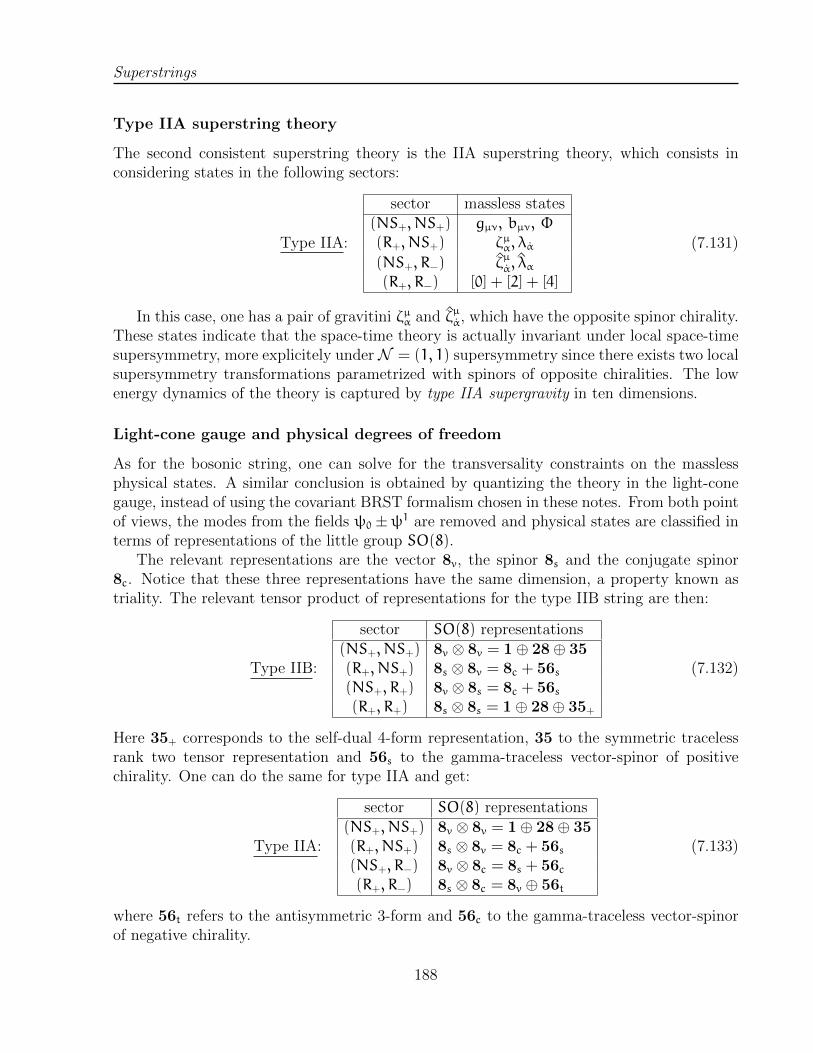
Superstrings
Type IIA superstring theory
The second consistent superstring theory is the IIA superstring theory, which consists inconsidering states in the following sectors:
Type IIA:
sector massless states(NS+, NS+) gµν, bµν, Φ
(R+, NS+) ζµα, λα(NS+, R−) ζµα, λα(R+, R−) [0] + [2] + [4]
(7.131)
In this case, one has a pair of gravitini ζµα and ζµα, which have the opposite spinor chirality.These states indicate that the space-time theory is actually invariant under local space-timesupersymmetry, more explicitely under N = (1, 1) supersymmetry since there exists two localsupersymmetry transformations parametrized with spinors of opposite chiralities. The lowenergy dynamics of the theory is captured by type IIA supergravity in ten dimensions.
Light-cone gauge and physical degrees of freedom
As for the bosonic string, one can solve for the transversality constraints on the masslessphysical states. A similar conclusion is obtained by quantizing the theory in the light-conegauge, instead of using the covariant BRST formalism chosen in these notes. From both pointof views, the modes from the fields ψ0 ±ψ1 are removed and physical states are classified interms of representations of the little group SO(8).
The relevant representations are the vector 8v, the spinor 8s and the conjugate spinor8c. Notice that these three representations have the same dimension, a property known astriality. The relevant tensor product of representations for the type IIB string are then:
Type IIB:
sector SO(8) representations(NS+, NS+) 8v ⊗ 8v = 1⊕ 28⊕ 35(R+, NS+) 8s ⊗ 8v = 8c + 56s(NS+, R+) 8v ⊗ 8s = 8c + 56s(R+, R+) 8s ⊗ 8s = 1⊕ 28⊕ 35+
(7.132)
Here 35+ corresponds to the self-dual 4-form representation, 35 to the symmetric tracelessrank two tensor representation and 56s to the gamma-traceless vector-spinor of positivechirality. One can do the same for type IIA and get:
Type IIA:
sector SO(8) representations(NS+, NS+) 8v ⊗ 8v = 1⊕ 28⊕ 35(R+, NS+) 8s ⊗ 8v = 8c + 56s(NS+, R−) 8v ⊗ 8c = 8s + 56c(R+, R−) 8s ⊗ 8c = 8v ⊕ 56t
(7.133)
where 56t refers to the antisymmetric 3-form and 56c to the gamma-traceless vector-spinorof negative chirality.
188

Superstrings
7.5 One-loop vacuum amplitudes
A strong consistency constraint for the superstring theories that we constructed, type IIAand type IIB, is provided by modular invariance of the one-loop vacuum amplitude.
The integrand of the modular integral over the torus modulus is the product of thecontribution from the xµ and (b, c) ghosts, that we computed earlier, giving (for d = 10)
Zx,g(τ, τ) =iV10
(4π2α ′)51(√
τ2η(τ)η(τ))8 (7.134)
and the contribution from the fermionic fields ψµ and from the (β, γ) superghosts that weconsider below.
The one-loop amplitude for both the fermions and the superghosts split into sectorsaccording to the boundary conditions for the fields. The Euclidean two-torus is parameterizedby a pair of coordinates σ1 and σ2 with periodicities (σ1, σ2) ∼ (σ1, σ2) + 2π(n+mτ1,mτ2).Along both of these one-cycles, one can specify whether the fields are periodic and anti-periodic.
The periodicity along the space cycle parametrized by σ1 was discussed already. It cor-responds to the choice of Ramond (periodic) or Neveu-Schwarz (anti-periodic) boundaryconditions:
ψµ(σ1 + 2π, σ2) = (−1)1−aψµ(σ1, σ2) , (7.135)
with a = 0 (resp. a = 1) in the NS (resp. R) sector.The periodicty along the Euclidean time direction was also indirectly considered in subsec-
tion 6.3.2. We have seen that, for fermionic fields the path integral with periodic boundaryconditions was corresponding to the trace of (−1)F exp−βH, while the partition functionitself, or trace over exp−βH, was given by the path integral with anti-periodic boundaryconditions. In other words, one considers the periodicity
ψµ(σ1 + 2πτ1, σ2 + 2πτ2) = (−1)1−bψµ(σ1, σ2) , (7.136)
for a path integral corresponding in the Hamiltonian formalism to an insertion of (−1)bF inthe trace.
7.5.1 Zero-modes
At a more abstract level, when one defines two-dimensional fermions on a genus zero surface,one needs to specify the spin structure, which is a four-fold choice of periodicities along bothone-cycles: (A,A), (A, P), (P,A) and (P, P) where A stands for anti-periodic and P standsfor periodic. All the first three case are called even spin structures while the last one is calledan odd spin structure (even or odd refers to the number of zero modes of the Dirac operatormod two).
In terms of super-space coordinates (z, θ), a two-torus is defined by the following identi-fications
(z, θ) ∼ (z+ 2π, εθ) ∼ (z+ 2πτ, ε ′θ) , ε, ε ′ ∈ −1, 1 . (7.137)
189

Superstrings
where ε and ε ′ define the spin structure.An important aspect of the computation of the one-loop vacuum amplitude for the bosonic
string was the presence of zero-modes for the ghosts fields, associated with the moduli andthe conformal Killing vectors on the two-torus. In the present case, there cannot be anyfermionic zero mode for the even spin structures, because of the anti-periodicity along atleast a one-cycle, while for the odd spin structure there exists a single zero-mode, whichis a constant spinor. Accordingly, there exists, for odd spin structure, a single fermionicsupermodulus ρ on the two-torus, which can be used to define a more general periodicity
(z, θ) ∼ (z+ 2π, θ) ∼ (z+ 2πτ+ θρ, θ+ ρ) (7.138)
as well as a superconformal Killing spinor, which corresponds to a spinorial shift ξ:
(z, θ) 7→ (z+ θξ, θ+ ξ) . (7.139)
This moduli and superconformal Killing spinor cannot exist for even spin structures, as θρand θξ would not have then the right periodicity properties for a bosonic coordinate.
7.5.2 Partition functions in the NS sector
Let us consider first the partition function for a single chiral fermion ψ(z). We define thefollowing partition functions for each spin structure:
Z[0b
]= Trns
[(−1)bFqL0−1/48
], (7.140a)
Z[1b
]= Trr
[(−1)bFqL0−1/48
]. (7.140b)
We start by the partition function with (A,A) boundary conditions, i.e TrnseL0−1/48, which
is easy to compute. A general state is of the form
· · ·(ψ−3/2
)N2 (ψ−1/2
)N1|0〉ns (7.146)
where Ni ∈ 0, 1. It gives the following result
Z[00
](τ) = q−1/48
(1+ q1/2
) (1+ q3/2
)· · · = q−1/48
∞∏n=0
(1+ qn+1/2
). (7.147)
In terms of the theta-functions (7.141) and the Dedekind eta-function (6.55) it can be writtenas
Z[00
](τ) =
√ϑ[00
](τ, 0)
η(τ). (7.148)
Next we consider the partition function with (A, P) boundary conditions, which meansa trace in the NS sector with (−)F inserted inside the trace. We still consider states of the
190

Superstrings
The Jacobi theta-function with characteristics is an analytic function of two complexvariables τ ∈ H and υ ∈ C, depending on two parameters α,β ∈ R and defined as
ϑ[ab
](τ, υ) = e−iπa(υ−
b2)q
a2
8
∞∏n=1
(1+ e−iπbe2iπυqn−
1+a2
)(1+ e+iπbe−2iπυqn−
1−a2
)(1− qn)
(7.141)From its definition it is obvious that
ϑ[11
](τ, 0) = 0 . (7.142)
The theta function obeys the modular transformations
ϑ[ab
](τ+ 1, υ) = e−
iπ4a(a−2)ϑ
[a
a+b−1
](τ, υ) , (7.143a)
ϑ[ab
](−1/τ, υ/τ) =
√−iτe
iπ2ab+ iπ
τυ2ϑ[b−a
](τ, υ) . (7.143b)
It has also the periodicity properties
ϑ[a+2mb+2n
](τ, υ) = eiπna ϑ
[a+2mb+2n
](τ, υ) , m, n ∈ Z . (7.144)
Finally it satifies the completely non-trivial Jacobi abstruse identity
ϑ[00
]4(τ, υ) − ϑ
[01
]4(τ, υ) − ϑ
[10
]4(τ, υ) = −ϑ
[11
]4(τ, υ) . (7.145)
We often use the notation ϑ[ab
](τ) := ϑ
[ab
](τ, 0).
form (7.146), however one gets a minus sign for each oscillator mode present. Therefore onegets
Z[01
](τ) = q−1/48
(1− q1/2
) (1− q3/2
)· · · = q−1/48
∞∏n=0
(1− qn+1/2
), (7.149)
which can be written as
Z[01
](τ) =
√ϑ[01
](τ)
η(τ). (7.150)
A partition function in the NS+ sector is then defined as
Trns
(1+ (−1)F
2qL0−c/24
). (7.151)
Then we move to the (β, γ) ghosts, which are, in the NS sector, bosons with anti-periodicboundary conditions. We consider the trace with a (−)bF insertion, where b ∈ 0, 1. Generalstates are of the form
· · · (β−3/2)M2(γ−3/2)
N2(β−1/2)M1(γ−1/2)
N1 |−〉ns . (7.152)
191

Superstrings
The NS vacuum contributes to the partition function as
q1/2−c/24(−1)b = q1/24(−1)b , (7.153)
as the vacuum as superghost charge one and dimension one-half.Since the (β, γ) fields are bosons, the path integral with anti-periodic boundary conditions
(b = 1) along Euclidean time corresponds to the trace with a (−)F insertion, while periodicboundary conditions (b = 0) corresponds to the trace without a (−)F insertion. Here F
is identified with the superghost number mod two, hence counts the number of superghostoscillator modes mod two.
We consider then, for instance, the contribution from γ−1/2 oscillators to the partitionfunction with (−1)bF inserted. One gets
1+ (−1)b+1q1/2 + q+ (−1)b+1q3/2 − · · · = 1
1+ (−1)bq1/2. (7.154)
Doing the same for all oscillators of β and γ give s
Zsg[0b
]= (−1)bq1/24
(1
1+ (−1)bq1/2
)2(1
1+ (−1)bq3/2
)2· · ·
= (−1)bq1/24∞∏n=1
(1
1+ (−1)bqn−1/2
)2. (7.155)
In terms of the theta-functions, this is
Zsg[0b
]= (−1)b
η(τ)
ϑ[0b
](τ)
. (7.156)
We can give describe the combined contribution to the partition function of the D = 10fermions and (β, γ) ghosts in the NS+ sector. Putting together the contribution (7.150),(7.147) and (7.156) one obtains
Zψ,sgns+ (τ) =1
2
(ϑ[00
](τ)
η(τ)
)5η(τ)
ϑ[0b
](τ)
−
(ϑ[01
](τ)
η(τ)
)5η(τ)
ϑ[01
](τ)
=1
2
(ϑ[00
](τ)
η(τ)
)4−1
2
(ϑ[01
](τ)
η(τ)
)4. (7.157)
We remark that this is exactly the same as the contribution of eight fermions, with theprojection 1
2(1 − (−1)F). This can be understood as follows. The superghosts (β, γ) are
actually removing the contribution of two towers of ψµ oscillators, much as the (b, c) ghostsremove two towers of xµ oscillators. If we have used the light-cone gauge, we would havefound the same result as only transverse oscillators remain, the light-cone oscillators alongψ0 ±ψ1 being removed by the gauge choice.
192

Superstrings
What remains after the projection is the tower of oscillators built out of the affine primarystates ψi−1/2|0〉ns, i = 2, . . . , 10 , containing only states with N ∈ N+ 1/2. This is precisely
the character in the vector representation of the affine SO(8) algebra, as discussed in subsec-tion 4.2.3. Indeed in this context one acts on the affine primary in the vector representationswith modes of the currents Jij, which are integer-modded.
7.5.3 Partition functions in the R sector
Let us consider the partition function in the Ramond sector, i.e. with periodic boundaryconditions along the space circle. We start by considering directly d = 10 fermions with PAspin structure, which is
Z[10
](τ) = Trrq
L0−5/24 . (7.158)
Since we haven’t performed yet the GSO projection, the ground state |a〉r is in the reducibleMajorana representation of the ten-dimensional Clifford algebra, which has dimension 25 =32; it has conformal dimension h = 5/8 (see eq. (4.140). The contribution from the groundstates to the partition function, taking into account their degeneracy is therefore 32q5/8−5/24 =(2q1/12)5.
One way to analyze this result is to consider that all the Ramond ground states areobtained from the highest weight state in the spinorial representation by acting with thelowering operators (−ψ00 +ψ
10), (ψ
20 − iψ
30), etc...
Adding the contributions from all the oscillators ψµ−n with n > 1 is easy, and we get theresult
Zψ[10
](τ) = (2q1/12)5
((1+ q)(1+ q2) · · ·
)10=
(2q1/12
∞∏n=1
(1+ qn)2
)5. (7.159)
In terms of theta-functions, this is
Zψ[10
](τ) =
(ϑ[10
](τ)
η(τ)
)5. (7.160)
For the set of ten fermions with PP spin structure, the result of the computation isdeceptively simple. One is interested in computing:
Zψ[11
](τ) = Trr(−1)
FqL0−5/24 . (7.161)
Remember that the operator (−1)F was an extension of the chirality matrix Γ 11 to the fullHilbert space of the fermionic CFT. If we focus on the 32-dimensional ground state, we knowthat for each ground state of positive chirality there exists a ground state with oppositechirality. Hence the two contributions cancel each other and we are left with
Zψ[11
](τ) = 0 . (7.162)
193

Superstrings
Another way to see this is that the explicit computation would give
Zψ[11
](τ) =
(ϑ[11
](τ)
η(τ)
)5= 0 , (7.163)
following eqn. (7.142).Finally, we have to compute the contribution of the superghosts to the Ramond sector
partition function. We focus on the PA spin structure, since the PP spin structure will notcontribute to the full partition function at the end. The superghosts being bosons, anti-periodicity in Euclidean time means that we compute the trace with (−1)F inserted.
The superghost Ramond vacuum |−〉r is defined in eq. (7.75a) and has conformal dimen-sion h = −3/8, hence contributes to the trace as q−11/24+3/8 = q−1/12. The problem in thepresent case is there there is an infinite degeneracy of the ground states, as any state of theform
(γ0)N0 |−〉r (7.164)
will have the same energy as the ground state. Taking into account the (−1)F insertion, thecontribution from all these states of conformal dimension h = 3/8 needs to be regularized,giving the result
q−1/12 (1− 1+ 1− 1+ · · · ) = limε→0+ q−1/12
(1− qε + q2ε − q3ε + · · ·
)= lim
ε→0+ q−1/12 1
1+ qε
= q−1/12 1
2. (7.165)
For the reader that doubts of this result, a more convincing argument will be given later.From there we act with the various oscillators as usual. Because of the (−1)F insertion,
the action of γ−1 for instance gives the factor
1− q+ q2 + · · · = 1
1+ q(7.166)
Adding all the contributions from the action of the oscillators β−n and γ−n with n ∈ Z>0,one reaches the result
Zsg[10
](τ) =
1
2q1/12∏∞
n=1(1+ qn)2
(7.167)
In terms of theta-functions, one obtains then
Zsg[10
](τ) =
η(τ)
ϑ[10
](τ)
. (7.168)
To conclude, the full contribution from the fermions and the superghosts (β,γ) in theR+ and R− sectors are the same, as the term with PP boundary conditions gives a vanishing
194

Superstrings
result from eq. (7.142). One gets then
Zψ,sgr± (τ) =1
2Zψ[10
](τ)Zsg
[10
](τ) (7.169)
=1
2
(ϑ[10
](τ)
η(τ)
)4. (7.170)
As before this result can be understood from the point of view of representation theoryof the SO(8) affine algebra. Zr± corresponds respectively to the characters of the spinorand conjugate spinor representations of SO(8), which are both eight-dimensional, which isreflected in the degeneracy of the ground state in (7.169).
In order to discriminate the characters for the spinor and conjugate spinor representations,it is possible, from the point of view of representation theory, to consider a character for anon-trivial group element in the Cartan sugroup of SO(8) rather than the identity. It amountsto give non-zero values to the υ argument in each theta-function. One can write then:
Zr±(τ, υ`) =1
2η(τ)4
4∏`=1
ϑ[10
](τ, υ`)±
4∏`=1
ϑ[11
](τ, υ`)
. (7.171)
7.5.4 Partition functions of type II string theories
The full partition function of type II string theories are obtained by adding the contributionsfrom the various left and right sectors that we have considered before. For the type IIBsuperstring theory, we need to consider schematically
Ziib = Zns+,ns+ − Zr+,ns+ − Zns+,r+ + Zr+,r+ . (7.172)
Minus signs have be added to the second and third terms to respect spin-statistics: space-timefermions running into the loop should contribute to the partition function with a negativesign.
For the type IIA superstring theory, we have to reverse the GSO projection in the rightRamond sector and get:
Ziia = Zns+,ns+ − Zr+,ns+ − Zns+,r− + Zr+,r− . (7.173)
The fermion and superghost contribution to the partition function completely factorizesinto its holomorphic and anti-holomorphic parts, given that the associated field theories arechiral. One has thus the following structure:
Ziib(τ, τ) = Zx,g(τ, τ)
(Zψ,sgns+ (τ) − Zψ,sgr+
(τ))(Zψ,sgns+ (τ) − Zψ,sgr+
(τ)). (7.174a)
Ziia(τ, τ) = Zx,g(τ, τ)
(Zψ,sgns+ (τ) − Zψ,sgr+
(τ))(Zψ,sgns+ (τ) − Zψ,sgr−
(τ)). (7.174b)
195
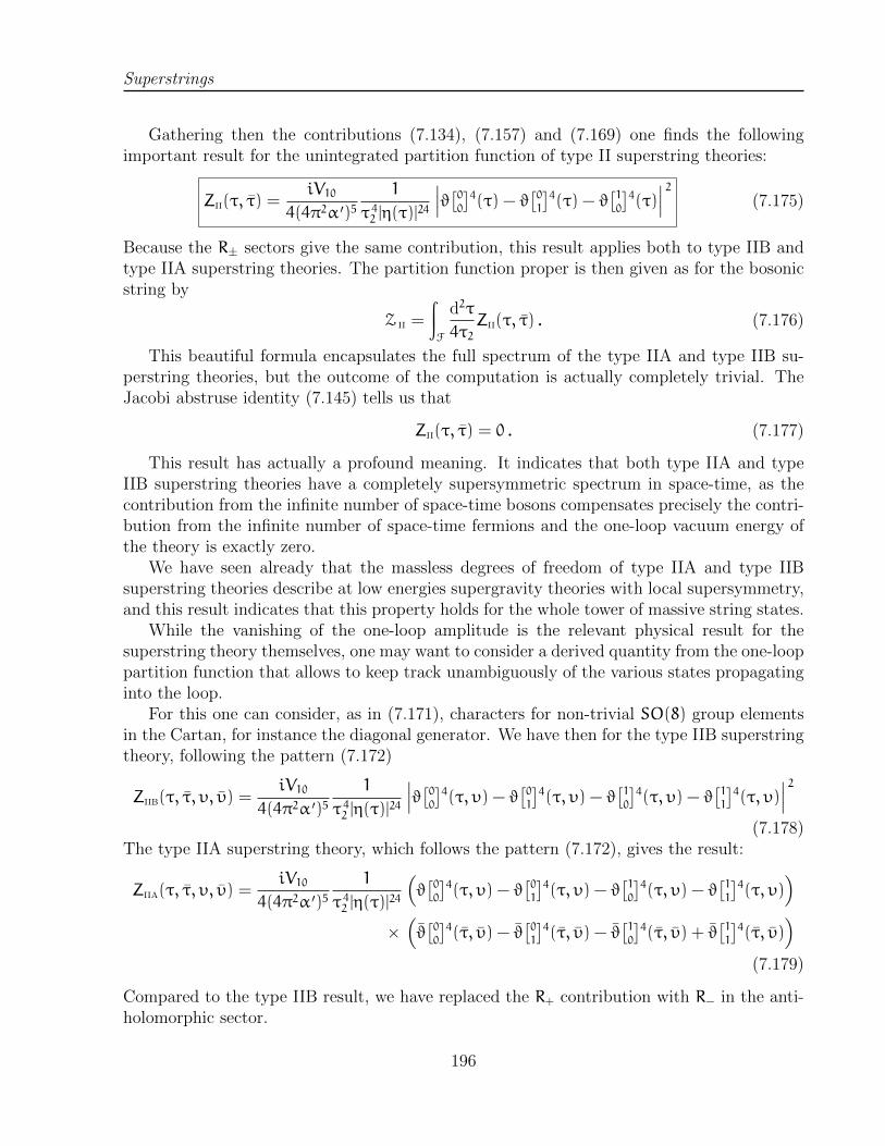
Superstrings
Gathering then the contributions (7.134), (7.157) and (7.169) one finds the followingimportant result for the unintegrated partition function of type II superstring theories:
Zii(τ, τ) =iV10
4(4π2α ′)51
τ 42 |η(τ)|24
∣∣∣ϑ[00]4(τ) − ϑ[01]4(τ) − ϑ[10]4(τ)∣∣∣ 2 (7.175)
Because the R± sectors give the same contribution, this result applies both to type IIB andtype IIA superstring theories. The partition function proper is then given as for the bosonicstring by
Z ii =
∫F
d2τ
4τ2Zii(τ, τ) . (7.176)
This beautiful formula encapsulates the full spectrum of the type IIA and type IIB su-perstring theories, but the outcome of the computation is actually completely trivial. TheJacobi abstruse identity (7.145) tells us that
Zii(τ, τ) = 0 . (7.177)
This result has actually a profound meaning. It indicates that both type IIA and typeIIB superstring theories have a completely supersymmetric spectrum in space-time, as thecontribution from the infinite number of space-time bosons compensates precisely the contri-bution from the infinite number of space-time fermions and the one-loop vacuum energy ofthe theory is exactly zero.
We have seen already that the massless degrees of freedom of type IIA and type IIBsuperstring theories describe at low energies supergravity theories with local supersymmetry,and this result indicates that this property holds for the whole tower of massive string states.
While the vanishing of the one-loop amplitude is the relevant physical result for thesuperstring theory themselves, one may want to consider a derived quantity from the one-looppartition function that allows to keep track unambiguously of the various states propagatinginto the loop.
For this one can consider, as in (7.171), characters for non-trivial SO(8) group elementsin the Cartan, for instance the diagonal generator. We have then for the type IIB superstringtheory, following the pattern (7.172)
Ziib(τ, τ, υ, υ) =iV10
4(4π2α ′)51
τ 42 |η(τ)|24
∣∣∣ϑ[00]4(τ, υ) − ϑ[01]4(τ, υ) − ϑ[10]4(τ, υ) − ϑ[11]4(τ, υ)∣∣∣ 2(7.178)
The type IIA superstring theory, which follows the pattern (7.172), gives the result:
Ziia(τ, τ, υ, υ) =iV10
4(4π2α ′)51
τ 42 |η(τ)|24
(ϑ[00
]4(τ, υ) − ϑ
[01
]4(τ, υ) − ϑ
[10
]4(τ, υ) − ϑ
[11
]4(τ, υ)
)×(ϑ[00
]4(τ, υ) − ϑ
[01
]4(τ, υ) − ϑ
[10
]4(τ, υ) + ϑ
[11
]4(τ, υ)
)(7.179)
Compared to the type IIB result, we have replaced the R+ contribution with R− in the anti-holomorphic sector.
196

Superstrings
7.5.5 Modular invariance of the superstring vacuum amplitude
An important consistency check of the validity of the construction outlined in this chapteris to show that the one-loop vacuum amplitude of the superstring theories satisfies modularinvariance. While this was done for the bosonic string, hence for the fields xµ and (b, c), wehave to understand what happens for fields ψµ and (β, γ). This is especially necessary as wehave considered a non-trivial separate GSO projection for the left-moving and right-movingdegrees of freedom.
Modular τ 7→ −1/τ transformation
We start by examining the behavior under the transformation τ 7→ −1/τ. Using equa-tions (7.143a) and (6.58) one has the following map:
ϑ[00
]4(−1/τ, υ/τ)
η4(−1/τ)= e
4iπυ2
τϑ[00
]4(τ, υ)
η4(τ)(7.180a)
ϑ[01
]4(−1/τ, υ/τ)
η4(−1/τ)= e
4iπυ2
τϑ[10
]4(τ, υ)
η4(τ)(7.180b)
ϑ[10
]4(−1/τ, υ/τ)
η4(−1/τ)= e
4iπυ2
τϑ[01
]4(τ, υ)
η4(τ)(7.180c)
ϑ[11
]4(−1/τ, υ/τ)
η4(−1/τ)= e
4iπυ2
τϑ[11
]4(τ, υ)
η4(τ)(7.180d)
Setting υ = 0, it implies that the combination of these factors that appears in the partitionfunction (7.175) is invariant under τ 7→ −1/τ as it should.
The relations (7.180) can be interpreted as follows. The transformation τ 7→ −1/τ in-terchanges the one-cycles of the two-torus, hence the spin structures. While the AA (firstequation) and PP (last equation) spin structures are invariant, the AP and PA spin struc-tures are exchanged. This is one way to see that a hypothetic string theory with only the(NS+, NS+) sector would inconsistent, as the Ramond sector would automatically appearfrom modular transformations.
One sees also that the minus sign in front of the R-NS and NS-R contributions in (7.172),that were justified by spin-statistics in space-time, are actually forced upon us by modularinvariance.
Modular τ 7→ τ+ 1 transformation
The transformation τ 7→ τ + 1 will also mix the different spin structures, as it correspondsto replacing the identification along Euclidean time z ∼ z + τ with z ∼ z + (τ + 1), therebyadding an extra twist of 2π along the spatial circle. Hence an AA spin structure will becomean AP spin structure, and an AP spin structure will become an AA spin structure. The
197

Superstrings
explicit computation gives (we removed the 1/η4 factor giving a common phase):
ϑ[00
]4(τ+ 1, υ) = ϑ
[01
]4(τ, υ) (7.181a)
ϑ[01
]4(τ+ 1, υ) = ϑ
[00
]4(τ, υ) (7.181b)
ϑ[10
]4(τ+ 1, υ) = −ϑ
[10
]4(τ, υ) (7.181c)
ϑ[11
]4(τ+ 1, υ) = −ϑ
[11
]4(τ, υ) (7.181d)
Hence
ϑ[00
]4 − ϑ
[01
]4 − ϑ
[10
]4 ± ϑ
[11
]4 7→ −
(ϑ[00
]4 − ϑ
[01
]4 − ϑ
[10
]4 ± ϑ
[11
]4)
(7.182)
and combining the holomorphic and anti-holomorphic contributions eliminates the extra mi-nus sign.
This completes the proof of the invariance of type IIA and type IIB superstring one-loopamplitudes under PSL(2,Z), the modular group of the two-torus.
198