lecture5 slides - princeton university · 5 mean field estimate for the radius of self-avoiding...
TRANSCRIPT

1
http://bioeng.princeton.edu/bioenginering-day/

MAE 545: Lecture 5 (10/1)Statistical mechanics of proteins
Dynamics of actin filaments and microtubules
(continued)

3
Stretching of worm-like chains
x
yz
F `p ⌧ kBT
~F
Small force Large forceF `p � kBT
hxi ⇡ L
2F `p
3kBThxi ⇡ L
"1�
skBT
4F `p
#
Approximate expression that interpolates between both regimes
J.F. Marko and E.D. Siggia, Macromolecules 28, 8759-8770 (1995)
F `p
kBT=
1
4
✓1� hxi
L
◆�2
� 1
4+
hxiL
~F

4
Steric interactionsSo far we ignored interactions between different chain segments, but in reality the chain cannot pass through itself due to steric interactions.
Example of forbidden configuration in 2D
Polymer chains are realizations of self-avoiding random walks!
Steric interactions are important for long polymers in the absence of pulling forces
~F
Steric interactions are not important in the presence
of pulling forces.

5
Mean field estimate for the radius of self-avoiding polymers
Paul Flory
RApproximate partition function: estimate number of self-avoiding random walks of N steps of size a that are restricted to a sphere of radius R.
Z(R,N) ⇡ gN ⇥ e�3R2/2Na2
[2⇡Na2/3]3/2⇥
1 ·
✓1� a3
R3
◆·✓1� 2a3
R3
◆· · ·
✓1� (N � 1)a3
R3
◆�
total number of random walks
reduction in entropy when constrained to sphere of radius R
}Cev
reduction in entropy due to
excluded volumeExcluded volume effect
lnCev =N�1X
k=1
ln
✓1� ka3
R3
◆⇡
N�1X
k=1
✓�ka3
R3� k2a6
2R6� · · ·
◆⇡ �N2a3
2R3� N3a6
6R6
Approximate partition function
lnZ(R,N) ⇡ N ln g � 3
2ln(2⇡Na2/3)� 3R2
2Na2� N2a3
2R3� N3a6
6R6

6
Relation between partition function and free energy
Paul Flory
R
Approximate partition function
lnZ(R,N) ⇡ N ln g � 3
2ln(2⇡Na2/3)� 3R2
2Na2� N2a3
2R3� N3a6
6R6
Statistical mechanicsZ =
X
c
e�Ec/kBT = e�G/kBT
reduction in entropy when constrained to sphere of radius R
G = �kBT lnZ
reduction in entropy due to excluded
volume interactions
}
Free energy cost for constraining polymer to sphere of radius R
�G(R,N) = Gent(R,N) +Gint(R,N)Gent(R,N) =
3kBTR2
2Na2
Gint(R,N) =kBTN2a3
2R3+
kBTN3a6
6R6
Estimate polymer radius by maximizing the partition function or equivalently by minimizing the free energy!

7
Mean field estimate for the radius of self-avoiding polymers
Paul Flory
RApproximate partition function
lnZ(R,N) ⇡ N ln g � 3
2ln(2⇡Na2/3)� 3R2
2Na2� N2a3
2R3� N3a6
6R6
Estimate polymer radius by maximizing the partition function
(higher order term can be
ignored)
R ⇠ aN⌫ ⇠ `p
✓L
`p
◆⌫
⌫ = 3/5Flory exponent
non-avoidingrandom walks
⌫ = 1/2
Exact result from more sophisticated methods
⌫ ⇡ 0.591R
lnZ
N ln g
@ lnZ(R,N)
@R⇡ � 3R
Na2+
3
2
N2a3
R4= 0

8
Self-avoiding walks in d dimensionsPaul Flory
R
Approximate partition function
Estimate R by maximizing the partition function
R ⇠ aN⌫ ⌫ =3
d+ 2
For Flory exponent is , but for non-avoiding walk .d � 4 ⌫ 1/2 ⌫ = 1/2
Z(R,N) ⇡ gN ⇥ e�dR2/2Na2
[2⇡Na2/d]d/2⇥1 ·
✓1� ad
Rd
◆·✓1� 2ad
Rd
◆· · ·
✓1� (N � 1)ad
Rd
◆�
lnZ(R,N) ⇡ N ln g � d
2ln(2⇡Na2/d)� dR2
2Na2� N2ad
2Rd
@ lnZ(R,N)
@R⇡ � dR
Na2+
d
2
N2ad
Rd+1= 0
What is then the expected scaling for radius R?

9
Self-avoiding walks in d dimensionsPaul Flory
R
Approximate partition function
Estimate free energy contributions when
lnZ(R,N) ⇡ N ln g � d
2ln(2⇡Na2/d)� dR2
2Na2� N2ad
2Rd
R ⇠ aN1/2
Gent = kBTdR2
2Na2⇠ kBT
Gint = kBTN2ad
2Rd⇠ kBTN
(4�d)/2Excluded volume interactions are only important for d < 4!
R
lnZ
N ln g
d
⌫
1 2 3 � 4
1 3/4 3/5 1/2
Note: except for d=3 these exponents are exact!
Flory estimate
R ⇠ aN⌫⌫ =
3
d+ 2
⌫ =1
2
d 4
d � 4

10
Interacting polymers
Now let us include also other interactions between polymer chains, e.g. van der Waals interactions. Interactions are typically attractive and their
magnitude can be modulated by the choice of solvent.
U(r)
0 ra
excludedvolume
good solvent(weak attraction)
bad solvent (strong attraction)

11
Interacting polymers
R
U(r)
0 ra
excludedvolume
good solvent(weak attraction)
bad solvent (strong attraction)
Mean field approximation for the total attraction energy
polymer density
Assuming uniform polymer density
Flory-Huggins parameter
Eatt =N2
2V
Z
r>ad3~r U(~r) ⌘ �kBT�N
2a3/R3
⇢(~r) = N/V ⇠ N/R3
⇢(~r)Eatt =
1
2
X
i 6=j
U(~ri � ~rj) ⇡1
2
Zd3~rd3~r0⇢(~r)⇢(~r0)U(~r � ~r0)
� = �Rr>ad
3~rU(~r)
2a3kBTExcluded volume effects will be treated separately.

12
Interacting polymersMean field approximation for the partition function
R
Z(R,N) ⇡ gN ⇥ e�3R2/2Na2
[2⇡Na2/3]3/2⇥
1 ·
✓1� a3
R3
◆·✓1� 2a3
R3
◆· · ·
✓1� (N � 1)a3
R3
◆�⇥ e�Eatt/kBT
lnZ(R,N) ⇡ N ln g � 3
2ln(2⇡Na2/3)� 3R2
2Na2� N2a3
2R3� N3a6
6R6+ �N2 a
3
R3
attraction
lnZ(R,N) ⇡ N ln g � 3
2ln(2⇡Na2/3)� 3R2
2Na2�
✓1
2� �
◆N2a3
R3� N3a6
6R6
Note: is typically a decreasing function of temperature and the coefficient in equation above changes sign at the so called temperature, where .
(1/2� �)
�(T )
�(✓) = 1/2✓
At large temperatures, where , polymers are in swollen coil state.� < 1/2
average density ⇢ ⇠ N
R3⇠ N�4/5 ! 0R ⇠ (1/2� �)1/5aN3/5
Exactly at temperature, where , attractive interactions and excluded volume are balanced.
✓ � = 1/2
R ⇠ aN1/2 average density ⇢ ⇠ N�1/2 ! 0
13
4
Good solvent – theta solventfrom Rubinstein, Colby. Data compiled by L.J. Fetters, J. Phys. Chem. 1994
polystyrene in benzene (good solvent)
59.02/1
2 ~ NRg
polystyrene in cyclohexane (theta solvent)
50.02/1
2 ~ NRg
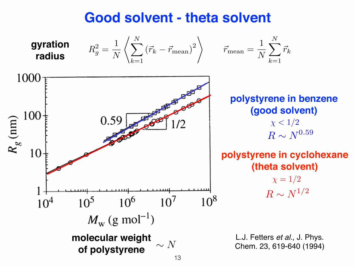
The swelling of the chain in good solvent results as a balance of the• repulsion energy between monomers and • the entropy loss due to increased end-to-end vector
Good solvent - theta solvent
polystyrene in benzene (good solvent)
� < 1/2
R ⇠ N0.59
polystyrene in cyclohexane (theta solvent)
� = 1/2
R ⇠ N1/2
molecular weight of polystyrene ⇠ N
L.J. Fetters et al., J. Phys. Chem. 23, 619-640 (1994)
R2g =
1
N
*NX
k=1
(~rk � ~rmean)2
+~rmean =
1
N
NX
k=1
~rkgyration radius

14
Swollen coil to globule transition
R
At low temperatures, where , polymersare in compact globule state with finite density
� > 1/2⇢ ⇠ N/R3
lnZ(R,N)
N⇡ ln g � 3R2
2N2a2�
✓1
2� �
◆Na3
R3� N2a6
6R6
(higher order term can be ignored)
Average density of the compact globule is obtained by maximizing entropy
lnZ(⇢, N)
N⇡ ln g +
✓�� 1
2
◆⇢a3 � ⇢2a6
6
⇢ ⇠✓�� 1
2
◆a�3
⇢a3
T
1
✓
Coil-Globule Transitionin Single Polymer Molecules.
If polymer chains are not ideal, interactions of non-neighboring monomer units (the so-called volume interactions) should be taken into account. If these interactions are repulsive, the coil swells with respect to its ideal dimensions. If monomer units attract each other, contraction leads to the “condensation” of polymer chain upon itself with the formation of a ”dense droplet” conformation, which is called a polymer globule.
the coil-globule transition
compact globule
swollencoil
lnZ/N
⇢0
ln g� > 1/2
� < 1/2� = 1/2

15
Swollen coil to globule transition
S.T. Sun et al., J. Chem. Phys. 73, 5971 (1980)
R2g =
1
N
*NX
k=1
(~rk � ~rmean)2
+
~rmean =1
N
NX
k=1
~rk
gyration radius
hydrodynamic radius
Rh =kBT
6⇡⌘D
polystyrene in cyclohexane

16
Further reading

17
Dynamics of actin filaments and microtubules
Actin filament
Microtubule

18
Cytoskeleton in cells
Actin filament
Microtubule
(wikipedia)
Cytoskeleton matrix gives the cell shape and mechanical resistance to deformation.

19
Crawling of cells
David Rogers, 1950s
Immune system:neutrophils chasing bacteria
migration of skin cells during wound healing
spread of cancer cells during metastasis of tumors
amoeba searching for foodv ⇠ 0.1µm/s

20
Movement of bacteria
Julie Theriot
Listeria monocytogenesmoving in PtK2 cells
(speeded up 150x)
Actin
L. A. Cameron et al., Nat. Rev. Mol. Cell Biol. 1, 110 (2000)
v ⇠ 0.1� 0.3µm/s

21
Molecular motors
A.B. Kolomeisky, J. Phys.: Condens. Matter 25, 463101 (2013)
Actin
Microtubule
Actin
Transport of large molecules around cells
(diffusion too slow)
Contraction of muscles
Harvard BioVisions
v ⇠ 1µm/s

22
Cell division
Segregation of chromosomesContractile ring divides
the cell in two
Microtubules Actin

23
Swimmingof sperm
cells
Jeff Guasto
Swimming of Chlamydomonas
(green alga)
Jeff Guasto
Bending is produced by motors walking on neighboring microtubule-like structures
v ⇠ 60µm/sv ⇠ 50µm/s

24
7nm
Actin filaments
Persistence length `p ⇠ 10µm
Minus end(pointed end)
Plus end(barbed end)
Typical length L . 10µm
Actin treadmilling

Dynamic fi laments423
Fig. 11.12 (a) If [ M ] c + = [ M ] c
− , both fi lament ends grow or shrink simultaneously. (b) If [ M ] c
+ ≠ [ M ] c − , there is
a region where one end grows while the other shrinks. The vertical line indicates the steady-state
concentration [ M ] ss where the fi lament length is constant.
the same time as the minus end shrinks. A special case occurs when the two
rates have the same magnitude (but opposite sign): the total fi lament length
remains the same although monomers are constantly moving through it.
Setting d n + /d t = −d n − /d t in Eqs. (11.5), this steady-state dynamics occurs at
a concentration [ M ] ss given by
[ M ] ss = ( k off + + k off
− ) / ( k on + + k on
− ). (11.7)
Here, we have assumed that there is a source of chemical energy to phos-
phorylate, as needed, the diphosphate nucleotide carried by the protein
monomeric unit; this means that the system reaches a steady state, but not
an equilibrium state.
The behavior of the fi lament in the steady-state condition is called tread-
milling, as illustrated in Fig. 11.13 . Inspection of Table 11.1 tells us that
treadmilling should not be observed for microtubules since the critical con-
centrations at the plus and minus ends of the fi lament are the same; that
is, [ M ] c + = [ M ] c
− and the situation in Fig. 11.12(a) applies. However, [ M ] c − is
noticeably larger than [ M ] c + for actin fi laments, and treadmilling should
occur. If we use the observed rate constants in Table 11.1 for ATP-actin
solutions, Eq. (11.7) predicts treadmilling is present at a steady-state actin
concentration of 0.17 µ M , with considerable uncertainty. A direct meas-
ure of the steady-state actin concentration under not dissimilar solution
conditions yields 0.16 µ M (Wegner, 1982 ). At treadmilling, the growth rate
from Eqs. (11.5) is
d n + /d t = −d n − /d t = ( k on + • k off
− – k on − • k off
+ ) / ( k on + + k on
− ), (11.8)
corresponding to d n + /d t = 0.6 monomers per second for [ M ] ss = 0.17 µ M .
25
Actin growth
k+on
k+o↵
k�o↵
k�on
dn�
dt= k�
on
[M ]� k�o↵
dn+
dt= k+
on
[M ]� k+o↵
growth of minus end growth of plus end
concentration of free actin monomers
no growth at no growth at
[M ]+c =k+o↵
k+on
[M ]�c =k�o↵
k�on
actin growsactin shrinks
Steady state regime
dn+
dt= �dn�
dt
front speeddn+
dt=
k+on
k�o↵
� k�on
k+o↵
k+on
+ k�on
⇡ 0.6s�1
[M ]ss
=k+o↵
+ k�o↵
k+on
+ k�on
⇡ 0.17µM

26
Distribution of actin filament lengths
k+on
k+o↵
k�o↵
k�on
total rate of actin monomer addition
kon
= k+on
+ k�on
ko↵
= k+o↵
+ k�o↵
total rate of actin monomer removal
Master equation@p(n, t)
@t= k
on
[M ]p(n� 1, t) + ko↵
p(n+ 1, t)� kon
[M ]p(n, t)� ko↵
p(n, t)
Continuum limit@p(n, t)
@t= �v
@p(n, t)
@n+D
@2p(n, t)
@n2
v = kon
[M ]� ko↵
D = (kon
[M ] + ko↵
)/2
drift velocitydiffusion constant
at large concentrations actin grows ( )
[M ] >ko↵
kon
= [M ]ss
v > 0
at low concentrations actin shrinks ( ) v < 0
[M ] <ko↵
kon
= [M ]ss

27
Distribution of actin filament lengths
k+on
k+o↵
k�o↵
k�on
total rate of actin monomer addition
kon
= k+on
+ k�on
ko↵
= k+o↵
+ k�o↵
total rate of actin monomer removal
What is steady state distribution of actin filament lengths at low concentration?
D = (kon
[M ] + ko↵
)/2
drift velocitydiffusion constant
@p⇤(n, t)
@t= �v
@p⇤(n, t)
@n+D
@2p⇤(n, t)
@n2= 0
v = kon
[M ]� ko↵
< 0
p⇤(n) =|v|D
e�|v|n/D =1
ne�n/n
n =D
|v| =(k
o↵
+ kon
[M ])
2(ko↵
� kon
[M ])average actin
filament length

28
Actin filament growing against the barrierwork done against the barrier for insertion of
new monomer
W = Fa
effective monomer free energy potential without barrier
away fromfilament
attachedto the tip
�
k+on
⇠ 4⇡D3
a
k+o↵
/ e��/kBT
effective monomer free energy potential with barrier
�
W
away fromfilament
attachedto the tip
k+on
(F ) ⇠ k+on
e�Fa/kBT
k+o↵
(F ) ⇠ k+o↵
F
k+on
(F )
k+o↵
(F )
2a
��W

29
Actin filament growing against the barrierwork done against the barrier for insertion of
new monomer
W = Fa
effective monomer free energy potential with barrier
�
W
away fromfilament
attachedto the tip
Growth speed of the tip
k+on
(F ) ⇠ k+on
e�Fa/kBT
k+o↵
(F ) ⇠ k+o↵
v+(F ) = k+on
[M ]e�Fa/kBT � k+o↵
Maximal force that can be balanced by growing filament
v+(Fmax
) = 0 Fmax
=kBT
aln
✓k+on
[M ]
k+o↵
◆
F
k+on
(F )
k+o↵
(F )
2a