lecture4 edges binary - department of computer … [luis von ahn et al. example using binary image...

9/10/2009

1

Edges and Binary Image Analysis

Thursday, Sept 10Kristen Grauman

UT-Austin

Previously• Filters allow local image neighborhood to influence our

description and features– Smoothing to reduce noise (before)

– Derivatives to locate contrast, gradient

• Filters have highest response on neighborhoods that g p g“look like” it; can be thought of as template matching.

• Seam carving application: – use image gradients to measure “interestingness” or “energy”

– remove 8-connected seams so as to preserve image’s energy.

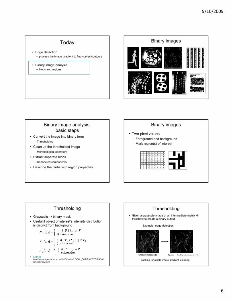
Today

• Edge detection– process the image gradient to find curves/contours

• Binary image analysis– blobs and regions

Edge detection• Goal: map image from 2d array of pixels to a set of

curves or line segments or contours.• Why?

• Main idea: look for strong gradients, post-process

Figure from J. Shotton et al., PAMI 2007

Figure from D. Lowe

Gradients -> edges

Primary edge detection steps:1. Smoothing: suppress noise2. Edge enhancement: filter for contrast3. Edge localization

Determine which local maxima from filter output are actually edges vs. noise

• Threshold, Thin

Smoothing with a GaussianRecall: parameter σ is the “scale” / “width” / “spread” of the Gaussian kernel, and controls the amount of smoothing.

…

9/10/2009

2

Effect of σ on derivatives

The apparent structures differ depending on Gaussian’s scale parameter.

Larger values: larger scale edges detectedSmaller values: finer features detected

σ = 1 pixel σ = 3 pixels

So, what scale to choose?It depends what we’re looking for.

Too fine of a scale…can’t see the forest for the trees.Too coarse of a scale…can’t tell the maple grain from the cherry.

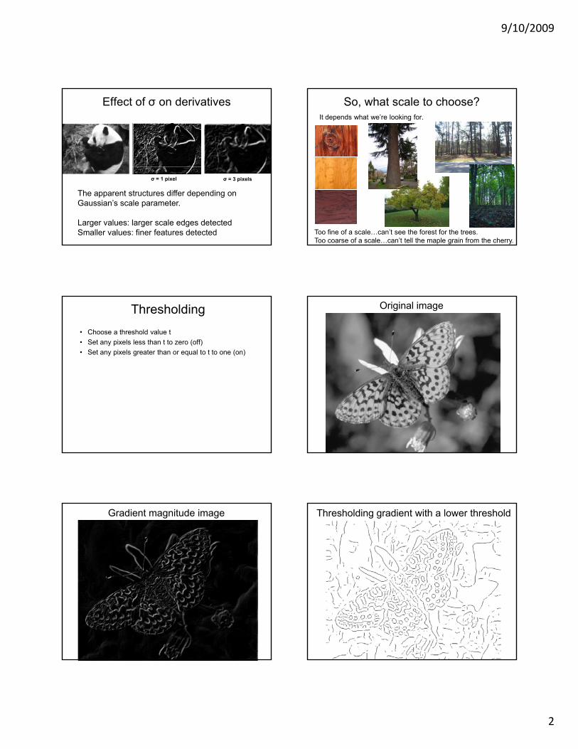
Thresholding• Choose a threshold value t• Set any pixels less than t to zero (off)• Set any pixels greater than or equal to t to one (on)

Original image

Gradient magnitude image Thresholding gradient with a lower threshold

9/10/2009

3

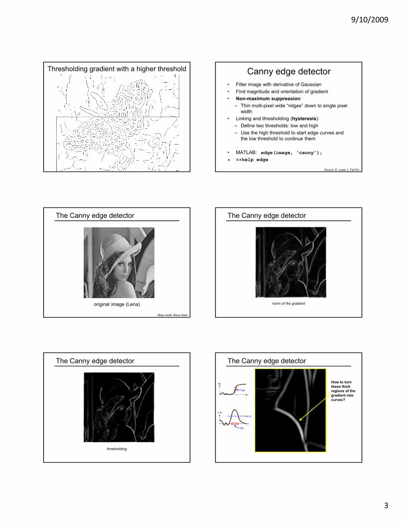
Thresholding gradient with a higher threshold Canny edge detector• Filter image with derivative of Gaussian • Find magnitude and orientation of gradient• Non-maximum suppression:

– Thin multi-pixel wide “ridges” down to single pixel width

Li ki d th h ldi (h t i )• Linking and thresholding (hysteresis):– Define two thresholds: low and high– Use the high threshold to start edge curves and

the low threshold to continue them

• MATLAB: edge(image, ‘canny’);• >>help edge

Source: D. Lowe, L. Fei-Fei

The Canny edge detector

original image (Lena)

Slide credit: Steve Seitz


norm of the gradient


thresholding


How to turn these thick regions of the gradient into curves?

thresholding

9/10/2009

4

Non-maximum suppression

Check if pixel is local maximum along gradient direction, select single max across width of the edge• requires checking interpolated pixels p and r

D. Forsyth


Problem:

thinning(non-maximum suppression)

Problem: pixels along this edge didn’t survive the thresholding

Hysteresis thresholding• Use a high threshold to start edge

curves, and a low threshold to continue them.

Source: Steve Seitz

Hysteresis thresholding

original imageoriginal image

high threshold(strong edges)

low threshold(weak edges)

hysteresis threshold

Source: L. Fei-Fei

Hysteresis thresholding

original image

high threshold(strong edges)

low threshold(weak edges)

hysteresis threshold

Object boundaries vs. edges

Background Texture Shadows

9/10/2009

5

Edges vs. human perception of contours

image human segmentation gradient magnitude

Berkeley segmentation database:http://www.eecs.berkeley.edu/Research/Projects/CS/vision/grouping/segbench/

Possible to learn from humans which combination of features is most indicative of a “good” contour?

[D. Martin et al. PAMI 2004] Human-marked segment boundaries

What features are responsible for perceived edges?

Feature profiles (oriented energy, brightness, color, and texture gradients) along the patch’s

[D. Martin et al. PAMI 2004]

the patch s horizontal diameter

What features are responsible for perceived edges?

Feature profiles (oriented energy, brightness, color, and texture gradients) along the patch’s


the patch s horizontal diameter


State-of-the-Art in Contour Detection

Prewitt, Sobel, Roberts

Canny

Canny+optthresholds

Learned with

Human agreement

Computer Vision GroupUC Berkeley Source: Jitendra Malik: http://www.cs.berkeley.edu/~malik/malik-talks-ptrs.html

combined features

9/10/2009

6

Today

• Edge detection– process the image gradient to find curves/contours

• Binary image analysis– blobs and regions

Binary images

Binary image analysis: basic steps

• Convert the image into binary form – Thresholding

• Clean up the thresholded imageM h l i l t– Morphological operators

• Extract separate blobs– Connected components

• Describe the blobs with region properties

Binary images

• Two pixel values– Foreground and background– Mark region(s) of interest

Thresholding

• Grayscale -> binary mask• Useful if object of interest’s intensity distribution

is distinct from background

• Examplehttp://homepages.inf.ed.ac.uk/rbf/CVonline/LOCAL_COPIES/FITZGIBBON/simplebinary.html

Thresholding• Given a grayscale image or an intermediate matrix

threshold to create a binary output.

Example: edge detection

Gradient magnitude

Looking for pixels where gradient is strong.

fg_pix = find(gradient_mag > t);

9/10/2009

7



Example: background subtraction

=-

Looking for pixels that differ significantly from the “empty” background.

fg_pix = find(diff > t);



Example: intensity-based detection

Looking for dark pixelsfg_pix = find(im < 65);



Example: color-based detection

Looking for pixels within a certain hue range.

fg_pix = find(hue > t1 & hue < t2);

A nice case: bimodal intensity histograms

Ideal histogram, light object on dark background

Actual observed histogram with noise

Images: http://homepages.inf.ed.ac.uk/rbf/CVonline/LOCAL_COPIES/OWENS/LECT2/node3.html

Not so nice cases

Shapiro and Stockman

Issues

• What to do with “noisy” binary outputs?– Holes– Extra small fragments

• How to demarcate multiple regions of interest? – Count objects– Compute further features per

object

9/10/2009

8

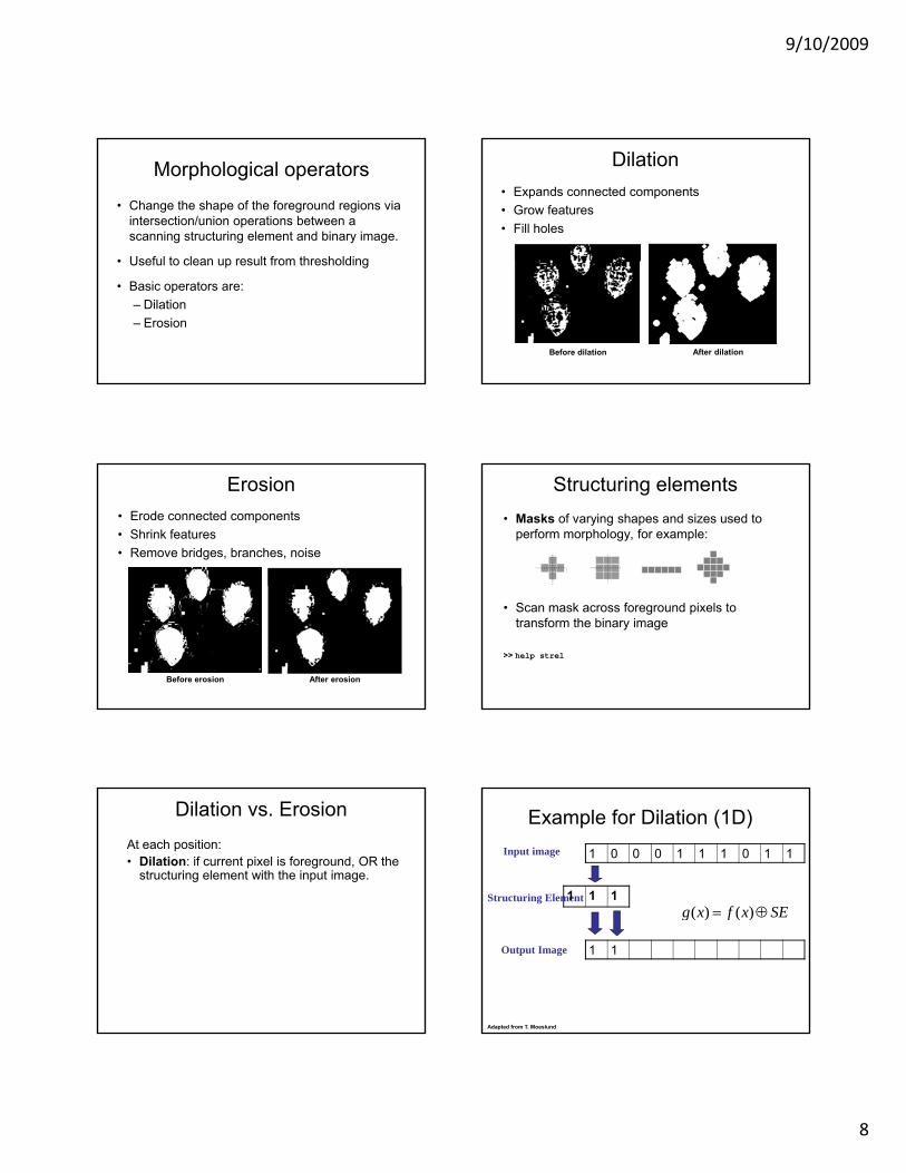
Morphological operators

• Change the shape of the foreground regions via intersection/union operations between a scanning structuring element and binary image.

• Useful to clean up result from thresholding• Useful to clean up result from thresholding

• Basic operators are:– Dilation– Erosion

Dilation• Expands connected components• Grow features• Fill holes

Before dilation After dilation

Erosion• Erode connected components• Shrink features• Remove bridges, branches, noise

Before erosion After erosion

Structuring elements• Masks of varying shapes and sizes used to

perform morphology, for example:

• Scan mask across foreground pixels to transform the binary image

>> help strel

Dilation vs. ErosionAt each position:• Dilation: if current pixel is foreground, OR the

structuring element with the input image.

Example for Dilation (1D)

SExfxg ⊕)()(

1 0 0 0 1 1 1 0 1 1Input image

Structuring Element 111SExfxg ⊕= )()(

1 1Output Image

Adapted from T. Moeslund

9/10/2009

9

Example for Dilation

1 0 0 0 1 1 1 0 1 1Input image

St t i El t 111Structuring Element

1 1Output Image

111


1 0 0 0 1 1 1 0 1 1Input image


1 1 0Output Image

111


1 0 0 0 1 1 1 0 1 1Input image


1 1 0 0Output Image

111


1 0 0 0 1 1 1 0 1 1Input image


1 1 0 1 1 1Output Image

111


1 0 0 0 1 1 1 0 1 1Input image


1 1 0 1 1 1 1Output Image

111


1 0 0 0 1 1 1 0 1 1Input image


1 1 0 1 1 1 1 1Output Image

111

9/10/2009

10


1 0 0 0 1 1 1 0 1 1Input image



111


1 0 0 0 1 1 1 0 1 1Input image


1 1 0 1 1 1 1 1 1 1Output Image

111

Note that the object gets bigger and holes are filled.>> help imdilate

2D example for dilation

Shapiro & Stockman

Dilation vs. ErosionAt each position:• Dilation: if current pixel is foreground, OR

the structuring element with the input image.• Erosion: if every pixel under the structuring

element’s nonzero entries is foreground, OR g ,the current pixel with S.

Example for Erosion (1D)

1 0 0 0 1 1 1 0 1 1Input image

St t i El t111

Structuring Element

0Output Image

SExfxg O)()( = _

Example for Erosion (1D)

1 0 0 0 1 1 1 0 1 1Input image

St t i El t111

Structuring Element

0 0Output Image

SExfxg O)()( = _

9/10/2009

11

Example for Erosion

1 0 0 0 1 1 1 0 1 1Input image


0 0 0Output Image

111

Example for Erosion

1 0 0 0 1 1 1 0 1 1Input image


0 0 0 0Output Image

111

Example for Erosion

1 0 0 0 1 1 1 0 1 1Input image


0 0 0 0 0Output Image

111

Example for Erosion

1 0 0 0 1 1 1 0 1 1Input image


0 0 0 0 0 1Output Image

111

Example for Erosion

1 0 0 0 1 1 1 0 1 1Input image


0 0 0 0 0 1 0Output Image

111

Example for Erosion

1 0 0 0 1 1 1 0 1 1Input image



111

9/10/2009

12

Example for Erosion

1 0 0 0 1 1 1 0 1 1Input image


0 0 0 0 0 1 0 0 0Output Image

111

Example for Erosion

1 0 0 0 1 1 1 0 1 1Input image


0 0 0 0 0 1 0 0 0 1Output Image

111

Note that the object gets smaller>> help imerode

2D example for erosion

Shapiro & Stockman

Opening• Erode, then dilate• Remove small objects, keep original shape

Before opening After opening

Closing• Dilate, then erode • Fill holes, but keep original shape

Before closing After closing

Applet: http://bigwww.epfl.ch/demo/jmorpho/start.php

Issues

• What to do with “noisy” binary outputs?– Holes– Extra small fragments

• How to demarcate multiple regions of interest? – Count objects– Compute further features per

object

9/10/2009

13

Connected components• Identify distinct regions of “connected pixels”

Shapiro and Stockman

Connectedness• Defining which pixels are considered neighbors

4-connected 8-connected

Source: Chaitanya Chandra

Connected components

• We’ll consider a sequential algorithm that requires only 2 passes over the image.

• Input: binary image• Input: binary image• Output: “label” image,

where pixels are numbered per their component

• Note: foreground here is denoted with black pixels.

Sequential connected components

Sequential connected components Connected components

Slide credit: Pinar Duygulu

9/10/2009

14

Region properties• Given connected components, can compute

simple features per blob, such as:– Area (num pixels in the region)– Centroid (average x and y position of pixels in the region)– Bounding box (min and max coordinates)

Circularity (ratio of mean dist to centroid over std)– Circularity (ratio of mean dist. to centroid over std)

A1=200A2=170

Circularity

Shapiro & Stockman

[Haralick]

Binary image analysis: basic steps (recap)

• Convert the image into binary form – Thresholding

• Clean up the thresholded imageM h l i l t– Morphological operators

• Extract separate blobs– Connected components

• Describe the blobs with region properties

Matlab• N = hist(Y,M)• L = bwlabel (BW,N);• STATS = regionprops(L,PROPERTIES) ;

– 'Area'– 'Centroid'

'BoundingBox'– 'BoundingBox' – 'Orientation‘, …

• IM2 = imerode(IM,SE);• IM2 = imdilate(IM,SE);• IM2 = imclose(IM, SE);• IM2 = imopen(IM, SE);

Example using binary image analysis: OCR

[Luis von Ahn et al. http://recaptcha.net/learnmore.html]

Example using binary image analysis: segmentation of a liver

Slide credit: Li Shen

9/10/2009

15

Example using binary image analysis:Bg subtraction + blob detection

…

Example using binary image analysis:Bg subtraction + blob detection

University of Southern Californiahttp://iris.usc.edu/~icohen/projects/vace/detection.htm

Binary images• Pros

– Can be fast to compute, easy to store– Simple processing techniques available– Lead to some useful compact shape descriptors

• Cons– Hard to get “clean” silhouettes– Noise common in realistic scenarios– Can be too coarse of a representation– Not 3d

Summary• Operations, tools Derivative filters

Smoothing, morphologyThresholdingConnected componentsMatched filtersHistograms

• Features, representations

Edges, gradientsBlobs/regionsColor distributionsLocal patternsTextures (next)

Histograms

Next

• Texture: read F&P Ch 9, Sections 9.1, 9.3

lecture4 edges binary - department of computer … [luis von ahn et al. example using binary image...

Documents