lecture notes series - applied mathematics · lecture notes series 1 numerical optimization...
TRANSCRIPT

Institute of Applied MathematicsMiddle East Technical University
LECTURE NOTES SERIES1
NUMERICAL OPTIMIZATIONConstrained Optimization
Bülent KarasözenGerhard-Wilhelm Weber
Design & Layout: Ömür Ugur

Preface
These are lecture notes offered to the students of the course Numerical Op-timization at the Institute of Applied Mathematics (IAM) of Middle EastTechnical University (METU) in Summer Semester 2003. In these months,this course was held for the first time at our new and for Turkey pioneeringinstitute which was founded in Autumn 2002. There has been the instituteteacher’s conviction that optimization theory is an important key technologyin many modern fields of application from science, engineering, operationalresearch and economy and, forthcoming, even in social sciences.
To be more precise, these lecture notes are prepared on the course’s sec-ond part which treated the case of constrained continuous optimization fromthe numerical viewpoint. Here, we pay attention to both the cases of lin-ear and nonlinear optimization (or: programming). In future, extensions ofthese notes are considered, especially in direction of unconstrained optimiza-tion. Herewith, our lecture notes are much more a service for the studentsthan a complete book. They essentially are a selection and a composition ofthree textbooks’ elaborations: There are the works “Lineare und Netzwerkop-timierung. Linear and Network Optimization. Ein bilinguales Lehrbuch” byH. Hamacher and K. Klamroth (2000) used in the parts about linear pro-gramming, “Linear and Nonlinear Programming” by S.G. Nash and A. Sofer(1996) and “Numerical Optimization” by J. Nocedal and S.J. Wright (1999)used for the parts about foundations and nonlinear programming.
During Summer Semester 2003, these lecture notes were given to thestudents in the handwritten form of a manuscript. We express our deepgratitude to Dr. Omur Ugur from IAM of METU for having prepared thisLATEX-typed version with so much care and devotion. Indeed, we are lookingforward that in future many of students of IAM will really enjoy these notesand benefit from them a lot. Moreover, we thank the scientific and institu-tional partners of IAM very much for the financial support which has madethe lecture notes in the present form possible.
With friendly regards and best wishes,
Bulent Karasozen and Gerhard-Wilhelm Weber,Ankara, in October 2003

ii

Contents
1 Introduction 1
1.1 Some Preparations . . . . . . . . . . . . . . . . . . . . . . . . 2
2 Linear Programming: Foundations and Simplex Method 9
3 Linear Programming: Interior-Point Methods 31
3.1 Introduction . . . . . . . . . . . . . . . . . . . . . . . . . . . . 31
3.2 Primal-Dual Methods . . . . . . . . . . . . . . . . . . . . . . . 32
3.3 A Practical Primal-Dual Algorithm . . . . . . . . . . . . . . . 40
4 Nonlinear Programming: Feasible-Point Methods 45
4.1 Linear Equality Constraints . . . . . . . . . . . . . . . . . . . 45
4.2 Computing the Lagrange Multipliers λ . . . . . . . . . . . . . 52
4.3 Linear Inequality Constraints . . . . . . . . . . . . . . . . . . 57
4.4 Sequential Quadratic Programming . . . . . . . . . . . . . . . 67
4.5 Reduced-Gradient Methods . . . . . . . . . . . . . . . . . . . 74
5 Nonlinear Programming: Penalty and Barrier Methods 81
5.1 Classical Penalty and Barrier Methods . . . . . . . . . . . . . 82

iv CONTENTS

List of Tables
2.1 Chocolate production. . . . . . . . . . . . . . . . . . . . . . . 10
2.2 Corner points and values. . . . . . . . . . . . . . . . . . . . . 12
4.1 SQP method . . . . . . . . . . . . . . . . . . . . . . . . . . . . 70
4.2 Reduced-gradient method. . . . . . . . . . . . . . . . . . . . . 78
5.1 Barrier function minimizers. . . . . . . . . . . . . . . . . . . . 87

vi LIST OF TABLES

List of Figures
2.1 Simplex algorithm, feasible region. . . . . . . . . . . . . . . . . 11
2.2 Simplex algorithm. . . . . . . . . . . . . . . . . . . . . . . . . 11
2.3 Feasible region. . . . . . . . . . . . . . . . . . . . . . . . . . . 16
2.4 Basis change. . . . . . . . . . . . . . . . . . . . . . . . . . . . 22
3.1 Central path, projected into x-space, showing a typical neigh-bourhood N . . . . . . . . . . . . . . . . . . . . . . . . . . . . 35
3.2 Iterates of Algorithm IPM2 plotted in (x, s)-space. . . . . . . . 40
3.3 Central path C, and a trajectory H from the current (noncen-tral) point (x, y, s) to the solution set Ω. . . . . . . . . . . . . 41
4.1 Sequence of movements in an active-set method. . . . . . . . . 61
4.2 Illustration of active-set algorithm. . . . . . . . . . . . . . . . 66
4.3 Zigzagging . . . . . . . . . . . . . . . . . . . . . . . . . . . . . 66
5.1 Effect of barrier term. . . . . . . . . . . . . . . . . . . . . . . 84
5.2 Contours of the logarithmic barrier function. . . . . . . . . . . 90

viii LIST OF FIGURES

Chapter 1
Introduction
In this chapter with its various aspects of consideration, we take into accountconstraints additionally to our problem of minimizing an objective functionf . Actually, we become concerned with the problem
(P)
minimize f(x)subject tohi(x) = 0 ∀i ∈ I := 1, 2, . . . , m ,gj(x) ≥ 0 ∀j ∈ J := 1, 2, . . . , s .
Here, f, hi and gj are supposed to be smooth real-valued function on Rn. By
smooth, we usually think of being one- or two-times continuously differen-tiable. The first group of constraints, where we demand . . . = 0, are calledequality constraints. The second group of constraints, where we ask . . . ≥ 0,are called inequality constraints. Denoting the feasible set, where we restrictthe objective function f on, by
M :=x ∈ R
n∣∣ hi(x) = 0 (i ∈ I), gj(x) ≥ 0 (j ∈ J)
,
our constrained optimization problem can be written as follows:
(P) minimize f(x) subject to x ∈M
or equivalently,
(P) minx∈M
f(x).

2 CHAPTER 1. INTRODUCTION
Depending on the context, namely on the various assumptions on f, h, g, Iand J we make, we shall sometimes denote the functions, the problem andits feasible set a bit differently or specific. For example, this will be the casewhen f, h, g are linear (to be more precise: linearly affine). In fact, we aregoing to distinguish the linear and the nonlinear case, speak about linearoptimization and nonlinear optimization. As in our course, the practicalcharacter and aspect of optimization is more emphasized than the analyticalor topological ones, we also talk about (non-)linear programming. This mayremind us of both the motivation of optimization by concrete applications,and the numerical solution algorithms. Because of the priority we gave to thenumerical-algorithmical aspect, we make the following introductory Sectionnot so long.
1.1 Some Preparations
By the following definition we extend corresponding notions from uncon-strained optimization almost straightforwardly:
Definition 1.1. Let a vector (or, point) x∗ ∈ Rn be given.
(i) We call x∗ a local solution of (P), if x∗ ∈ M and there is a neighbour-hood N (x∗) of x∗ such that
f(x∗) ≤ f(x) ∀x ∈M ∩N (x∗).
(ii) We call x∗ a strict local solution of (P), x∗ ∈ M and there is a neigh-bourhood N (x∗) of x∗ such that
f(x∗) < f(x) ∀x ∈(M ∩ N (x∗)
)\ x∗ .
(iii) We call x∗ an isolated local solution of (P), x∗ ∈ M and there is aneighbourhood N (x∗) of x∗ such that x∗ is the only local solution of(P) in M ∩ N (x∗).
Sometimes, we also say (strict or isolated) local minimizer for a (strict orlocal) local solution.
Do you understand and geometrically distinguish these three conditions?We shall deepen our understanding in the exercises and in the followingsections.

1.1. SOME PREPARATIONS 3
Example 1.1. Let us consider the problem
(P)
minimize
(f(x) :=
)x1 + x2
subject to x21 + x2
2 − 2 = 0(i.e., h(x) := x2
1 + x22 − 2
),
Here, | I | = 1 (h1 = h) and J = ∅. We see by inspection that the feasibleset M is the circle of radius
√2 centered at the origin (just the boundary
of the corresponding disc, not its interior). The solution x∗ is obviously(−1,−1)T , this is the global solution of (P): From any other point on thecircle, it is easy to find a way to move that stays feasible (i.e., remains on thecircle) while decreasing f . For instance, from the point (
√2, 0)T any move in
the clockwise direction around the circle has the desired effect. Would youplease illustrate this and the following graphically? Indeed, we see that atx∗, the gradient ∇h(x∗) is parallel to the gradient ∇f(x∗):
(
(11
)= ) ∇f(x∗) = λ∗∇h(x∗)
where λ∗ = λ∗1 = −12.
The condition found in the previous example to be necessary for a (local)minimizer (or, local minimum) can be expressed as follows:
∇xL(x∗, λ∗) = 0,
where L : Rn × R
m −→ R is defined by L(x, λ) := f(x) − λh(x) and calledthe Lagrange function. The value λ∗ is called the Lagrange multiplier (at x∗).This Lagrange multiplier rule is a first-order necessary optimality condition1 (NOC) which can be extended to cases where I is of some other cardi-nality m ≤ n. in fact, provided that the Linear Independence ConstraintQualification (a regularity condition) holds at x∗, saying that the gradients
∇h1(x∗),∇h2(x
∗), . . . ,∇hm(x∗),
regarded as a family (i.e., counted by multiplicity), are linearly independent,then there exist so-called Lagrange multipliers λ∗
1, λ∗2, . . . , λ
∗m such that
∇f(x∗) =
m∑
i=1
λ∗i∇h(x∗).
1In the next sections, we also consider feasibility to be a part of it.

4 CHAPTER 1. INTRODUCTION
The latter equation is just
∇xL(x∗, λ∗) = 0,
where L : Rn × R
m −→ R is the so-called Lagrange function L(x, λ) :=f(x) − λTh(x), with λ := (λ1, λ2, . . . , λm)T and h := (h1, h2, . . . , hm)T .
Next, we slightly modify Example 1.1. We replace the equality constraintby an inequality.
Example 1.2. Let us consider the problem
(P)
minimize
(f(x) :=
)x1 + x2
subject to 2 − x21 − x2
2 ≥ 0(i.e., g(x) := 2 − x2
1 − x22
),
here, I = ∅ and |J | = 1 (g = g1). The feasible set consists of the cir-cle considered in Example 1.1 and its interior. We note that the gradient∇g(x) = (−2x1,−2x2)
T points from the circle in direction of the interior.For example, inserting the point x = (
√2, 0)T gives ∇g(x) = (−2
√2, 0)T ,
pointing in the direction of the negative x1− axis, i.e., inwardly (regardedfrom x). By inspection, we see that the solution of (P) is still x∗ = (−1,−1)T ,and we have now
∇f(x∗) = µ∗∇g(x),where µ∗ = µ∗
1 = 12≥ 0.
Again, we can write our necessary equation by using a Lagrange function,namely, L(x, µ) := f(x) − µg(x):
∇xL(x∗, µ∗) = 0, where µ∗ ≥ 0.
Again, our necessary optimality condition can be generalized by admittinganother finite cardinality s of J , andm = | I | possibly to be positive (m ≤ n).For this purpose, we need a regularity condition (constraint qualification) atour local minimizer x∗, once again. In the presence of both equality andinequality constraints, we can again formulate LICQ. For this purpose, weintroduce the set of active inequality constraints at some feasible point x:
J0(x) :=j ∈ J
∣∣gj(x) = 0.
Then, LICQ at x∗ means the linear independence of the vectors (togetherregarded as a family)
1.1. SOME PREPARATIONS 5
∇hi(x∗) (i ∈ I), ∇gj(x
∗)(j ∈ J0(x
∗))
(so that the gradients of the active inequalities are taken into account to thegradients of the equality constraints, additionally). Another famous regular-ity condition is somewhat weaker than LICQ and called MFCQ (Mangasarian-Fromovitz Constraint Qualification). The geometrical meaning of MFCQ isthe following: At each point ofM we have an inwardly pointing direction (rel-ative to the surface given by the zero set of h). In the sequel, we refer to LICQfor simplicity. Now, our first-order necessary optimality conditions (NOC)are called Karush-Kuhn-Tucker conditions: There exist λ∗ = (λ∗1, . . . , λ
∗m)T
and µ∗ =(µ∗
j
)j∈J0(x∗)
such that
∇f(x∗) =m∑
i=1
λ∗i∇hi(x∗) +
∑
j∈J0(x∗)
µ∗j∇gj(x
∗),
µ∗j ≥ 0 ∀j ∈ J0(x
∗).
The second ones of the Lagrange multipliers, namely µ∗j (j ∈ J0(x
∗)), neces-sarily are nonnegative. Here, we may interpret this as by the existence of (rel-atively) inwardly pointing direction along which f does not decrease, whenstarting from our local minimizer x∗. Let us summarize our considerationby referring to the Lagrange function L(x, λ, µ) := f(x) − λTh(x) − µTg(x),where
(µ∗
j
)j∈J0(x∗)
is filled up by additional parameters µj (j 6∈ J0(x∗)) (at
x = x∗, we have µ∗j = 0, j 6∈ J0(x
∗)).
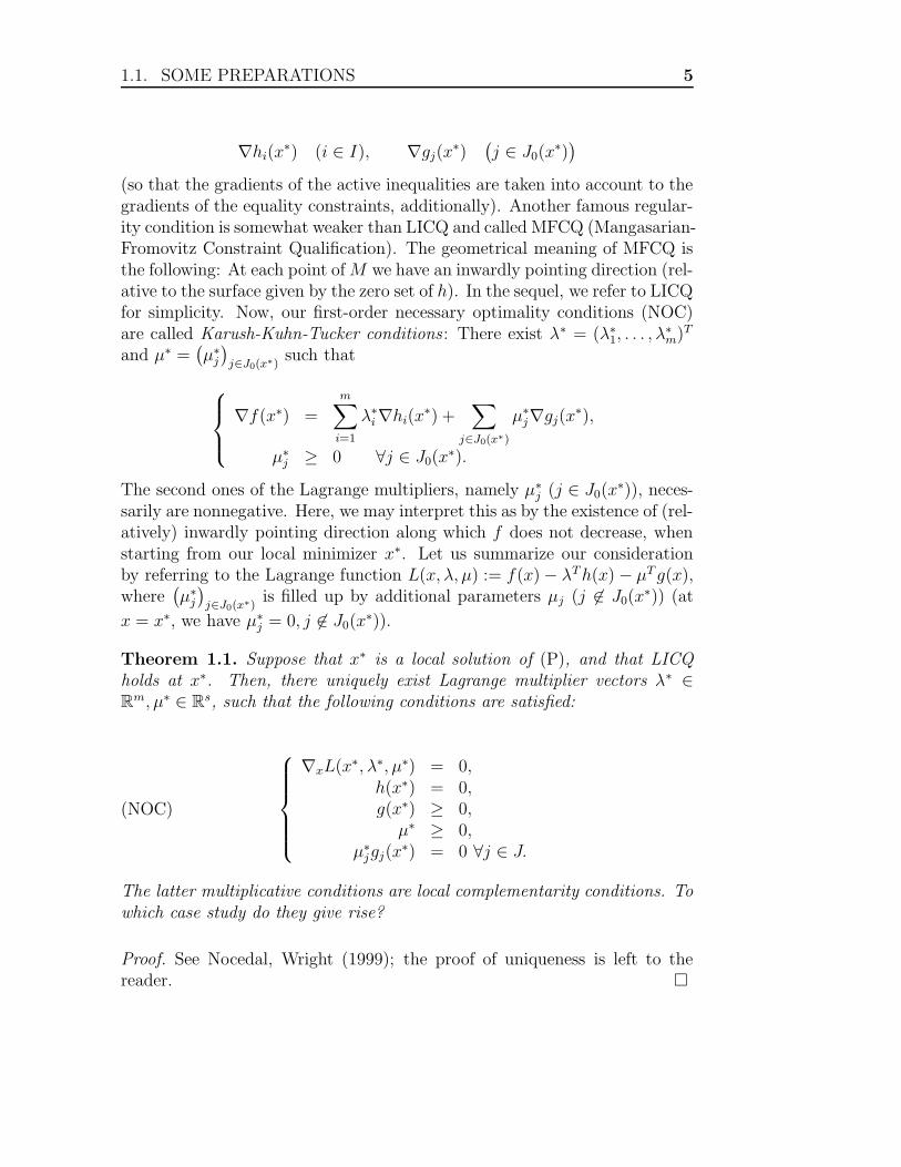
Theorem 1.1. Suppose that x∗ is a local solution of (P), and that LICQholds at x∗. Then, there uniquely exist Lagrange multiplier vectors λ∗ ∈R
m, µ∗ ∈ Rs, such that the following conditions are satisfied:
(NOC)
∇xL(x∗, λ∗, µ∗) = 0,h(x∗) = 0,g(x∗) ≥ 0,µ∗ ≥ 0,
µ∗jgj(x
∗) = 0 ∀j ∈ J.
The latter multiplicative conditions are local complementarity conditions. Towhich case study do they give rise?
Proof. See Nocedal, Wright (1999); the proof of uniqueness is left to thereader.

6 CHAPTER 1. INTRODUCTION
Often, the compact form of (NOC), where we do not explicitly refer tothe active inequalities j ∈ J0(x
∗), is more convenient. In other times, a directreference to J0(x
∗) is better for us. We note that our first-order necessaryoptimality conditions are not the only ones. In the subsequent sections and inthe presentation given in lectures, we shall briefly indicate them sometimes.These conditions are, more or less, generalization of the condition (taught tous in the unconstrained case) that the gradient vanishes at a local solution:∇f(x∗) = 0, if I = J = ∅. Provided that all the defining functions aretwice continuously differentiable, then we know the second-order optimalitycondition saying that the Hessian matrix has to be positive semi-definite:
ρT∇2xxf(x∗)ρ ≥ 0 ∀ρ ∈ R
n.
But how does this condition look like in our case of constrained optimization?Let us define the tangent space of M at x∗ as follows:
Tx∗ :=ρ ∈ R
n∣∣∇Thi(x
∗)ρ = 0 ∀i ∈ I, ∇Tgj(x∗)ρ = 0 ∀j ∈ J0(x
∗).
Then, our second-order condition states that the Hessian of the Lagrangefunction L at x∗ is positive semi-definite over Tx∗. Here, we take the vectorsρ ∈ R
n for left- or right-multiplication from Tx∗. This can also be expressedas the positive semi-definiteness of this Hessian, when firstly left- and right-multiplied by BT and B, respectively, over R
n. Here, B is any matrix whosecolumns constitute a basis of the linear space Tx∗. Herewith, we can expressour second-order optimality condition so, where n = n− m, m = |J0(x
∗) |:
(NOC)s.o. ρTBT∇2xxL(x∗, λ∗, µ∗)Bρ ≥ 0 ∀ρ ∈ R
bn.
In literature, we also find some refined condition, where in the statementof positive-definiteness the reference space Tx∗ is replaced by the set C•
x∗
which is a (tangent) cone. Namely, C•x∗ comes from substituting the gradient
conditions on the active inequalities by
∇Tgj(x∗)ρ = 0 ∀j ∈ J0(x
∗) with µ∗j > 0,
∇Tgj(x∗)ρ ≥ 0 ∀j ∈ J0(x
∗) with µ∗j = 0.

1.1. SOME PREPARATIONS 7
Theorem 1.2. Suppose that x∗ is a local solution of (P), and that LICQis satisfied at x∗. Let λ∗ and µ∗ be the corresponding Lagrange multipliervectors so that (NOC) is (necessarily) fulfilled.
Then, the Hessian ∇2xxL(x∗, λ∗, µ∗) is positive semi-definite over Tx∗, or
(refined version) over C•x∗.
Proof. See, e.g., Nash, Sofer (1996) and Nocedal, Wright (1999).
This theorem plays an important role for detecting that some found orsubmitted stationary point x∗ (i.e., x∗ fulfills our first-order necessary opti-mality conditions) is not a local solution, but a local minimizer or a saddlepoint. How can we use Theorem 1.2 for this purpose? A saddle point is inbetween of a local minimizer and a local maximizer: there are feasible direc-tions of both an increasing and a decreasing behaviour of f . But how can wedetect that a stationary point, i.e., a candidate for being a local minimizerreally is such a one? what we know from the unconstrained case gives rise toassume that we should turn from positive semi-definiteness (over Tx∗ or C•
x∗)to positive definiteness (over Tx∗ \ 0 or C•
x∗ \ 0). In fact, by this sharp-ening of (NOC)s.o. we obtain a condition which together with our first-order(NOC) is sufficient for x∗ to become a local solution. In particular, we arriveat
(SOC)s.o. ρTBT∇2xxL(x∗, λ∗, µ∗)Bρ > 0 ∀ρ ∈ R
bn \ 0 .
We state the following theorem on second-order sufficient optimality condi-tions:
Theorem 1.3. Suppose that for some point x∗ ∈M there are Lagrange mul-tiplier vectors λ∗, µ∗ such that the conditions (NOC) (of first-order) are satis-fied and µ∗
j > 0 (j ∈ J0(x∗)). Suppose also that the Hessian ∇2
xxL(x∗, λ∗, µ∗)is positive definite over Tx∗, or over C•
x∗ (i.e., over Tx∗ \ 0, or C•x∗ \ 0).
Then, x∗ is a strict local solution for (P).
Proof. See, e.g., Nash, Sofer (1996) and Nocedal, Wright (1999).
In our exercises, we shall consider a few examples on finding local orglobal solutions for nonlinear optimization problem, where the utilization ofnumerical-algorithmical methods is still not necessary. Let us also concludeour Section 1.1 with another such example.
Example 1.3. Let us consider the problem (P) from Example 1.2:

8 CHAPTER 1. INTRODUCTION
(P)
minimize
(f(x) :=
)x1 + x2
subject to 2 − x21 − x2
2 ≥ 0(i.e., g(x) := 2 − x2
1 − x22
).
We want to check the second-order conditions. The Lagrangian is
L(x, µ) := (x1 + x2) − µ(2 − x1 − x2),
and it is easy to show that the Karush-Kuhn-Tucker conditions (NOC) aresatisfied by x∗ = (−1,−1)T , with µ∗ = 1
2. The Hessian of L (with respect to
x) is
∇2xxL(x∗, µ∗) =
(2µ∗ 00 2µ∗
)=
(1 00 1
).
This matrix is positive definite, i.e., it satisfies ρT∇2xxL(x∗, µ∗)ρ > 0 for all
ρ ∈ Rn \ 0 (in particular, for all elements of Tx∗, C•
x∗, except 0). So, itcertainly satisfies the conditions of Theorem 1.3.
We conclude that x∗ = (−1,−1)T is a strict local solution for (P). Let usremark that x∗ is a even a global solution, since (P) is a convex programmingproblem.
In this course, we do not pay much attention to stability aspects which,however, can be well analyzed by LICQ and (SOC)s.o. Next, we concentrateof the linear case of (P).

Chapter 2
Linear Programming:Foundations and SimplexMethod
In this chapter, based on the book of Hamacher, Klamroth (2000), we con-sider easy examples which lead to optimization (“programming”) problems:Linear programs play a central role in modelling of optimization problems.
Example 2.1. The manufacturer “Chocolate & Co.” is in the process ofreorganizing its production. Several chocolate products which have beenproduced up to now are taken out off production and are replaced by twonew products. The first product P1 is fine cocoa, and the second one P2 isdark chocolate. The company uses three production facilities F1, F2, and F3for the production of the two products. In the central facility F1 the cocoabeans are cleaned, roasted and cracked. In F2, the fine cocoa and in F3 thedark chocolate are produced from the preprocessed cocoa beans. Since thechocolate products of the company are known for their high quality, it canbe assumed that the complete output of the company can be sold on themarket. The profit per sold production unit of P1 (50kg of cocoa) is 3 (¤),whereas it is 5 per sold production unit of P2 (100kg of chocolate). However,the capacities of F1–F3 are limited as specified in Table 2.1.
(For example, the row corresponding to F1 implies that the per unit P1 andP2, 3% and 2%, respectively, of the daily capacity of production facility F1are needed, and that 18% of the daily capacity of F1 is available for theproduction of P1 and P2.)
The problem to be solved is to find out how many units x1 of productsP1 and x2 of product P2 should be produced per day in order to maximize

10CHAPTER 2. LINEAR PROGRAMMING: FOUNDATIONS AND
SIMPLEX METHOD
P1 P2 available capacity(in % of the daily capacity)
F1 3 2 18F2 1 0 4F3 0 2 12
Table 2.1: Chocolate production.
the profit (while satisfying the capacity constraints.) This problem can beformulated as a linear program (LP):
(LP)
maximize 3x1 + 5x2 =: cTxsubject to the constraints
3x1 + 2x2 ≤ 18 (I)x1 ≤ 4 (II)
2x2 ≤ 12 (III)x1, x2 ≥ 0 (IV), (V)
The function cTx is the (linear) objective function of the LP. The constraintsare partitioned into functional constraints ((I)–(III)) and nonnegativity con-straints ((IV),(V)). Each x which satisfies all the constraints, is called a fea-sible solution of the LP and cTx is its objective (function) value. Instead ofmaximizing the function, it is often minimized. In this case, the coefficientsci of the objective function can be interpreted as unit costs. The functionalconstraints can also be equations (“=”) or inequalities with “≥”.
Let us continue by introducing a graphical procedure for the solution of(LP). In a first step, we draw the set of feasible solutions (the feasible regionP) of (LP), that is the set of all points (vectors) (x1, x2), in matrix notation:(x1
x2
), satisfying all the constraints; see Figure 2.1.
If Aix ≤ bi is one of the constraints (e.g., Ai = (3, 2), b1 = 18) we draw theline corresponding to the equation
Aix = bi.
This space separates the space R2 into two half-spaces
Aix ≤ bi, and Aix ≥ bi
The set P of feasible solutions is a subset of the half-space Aix ≤ bi. Weobtain P by taking the intersection of all these half-spaces including the half-

11
Figure 2.1: Simplex algorithm, feasible region.
spaces x1 ≥ 0 and x2 ≥ 0. A set of points in R2, which is obtained in such a
way is called a convex polyhedron.
In a second step, we draw the objective function z := cTx = 3x1 + 5x2.For any given value of z we obtain a line, and for any two different valuesof z we obtain two parallel lines for which z is as large as possible. Thefollowing Figure 2.2 shows the feasible region P and, additionally, the linecorresponding to the objective function 3x1 +5x2, i.e., the line correspondingto the objective value z = 15. The arrow perpendicular to this line indicates,in which direction the line should be shifted in order to increase z.
Figure 2.2: Simplex algorithm.
The intersection of any line cTx = z with P in some x ∈ P corresponds
to a feasible solution x =
(x1
x2
)with objective value z. Hence, in order to
maximize the objective function, the line is shifted parallel as far as possiblewithout violating the condition

12CHAPTER 2. LINEAR PROGRAMMING: FOUNDATIONS AND
SIMPLEX METHOD
x ∈ R
2∣∣cTx = z
∩ P 6= ∅.
This just gives the line which passes through the point x∗ =
(26
). Hence,
z∗ = cTx∗ = 3 · 2 + 5 · 6 = 36 is the maximum possible profit.
As a consequence, the company “Chocolate & Co.” will produce 2 pro-duction units of cocoa and 6 production units of the dark chocolate per day.
In this example, we observe an important property of linear programs:There is always an optimal solution (i.e., a feasible solution for which cTx ismaximal) which is a corner point of P –or there is no optimal solution at all.This general property of LPs is a fundamental for the method introducedbelow as a general solution for LPs: the simplex method :
Imagine to move from corner point to corner point of P (a corner pointis an element of P which is an intersection of two or more of its facets)using a procedure which guarantees that the objective value is improved inevery step. As soon as we have reached a corner point in which no furtherimprovement of the objective value is possible, the algorithm stops and thecorner point corresponds to an optimal solution of the LP. In Example 2.1,such a sequence of corner points is, e.g., as stated in Table 2.2.
corner point objective value 3x1 + 5x2
1.
(00
)0
2.
(40
)12
3.
(43
)27
4.
(26
)36 (STOP), no further improvement possible.
Table 2.2: Corner points and values.
This is exactly the idea on which the simplex method is based, which wasdeveloped by G. Dantzig in 1947. It yields an optimal solution (whenever itexists) for only LP. An important step in the development of the precedingidea for arbitrary LPs is the application of methods from linear algebra.
Definition 2.1. A given LP is said to be in standard form if and only if itis given as

13
(LP)st
minimize cT
subject to Ax = bx ≥ 0 (i.e., xi ≥ 0 ∀i ∈ 1, . . . , n),
where A in an m × n matrix, m ≤ n, and rank(A) := dim(ImT ) = m (Tbeing the linear transformation represented by A relative to standard bases).
If m ≤ n or rank(A) = m are not the case, then we can reintroducem ≤ n, rank(A) =: m by omitting redundant (i.e., linearly on other m onesdepending) constraints. In the following, we show how any given LP can betransformed into standard form.
Assume that an LP in general form is given:
(LP)gf
minimize c1x1 + · · · + cnxn
subject to ai1x1 + · · ·+ ainxn = bi (i ∈ 1, . . . , p)ai1x1 + · · ·+ ainxn ≤ bi (i ∈ p+ 1, . . . , q)ai1x1 + · · ·+ ainxn ≥ bi (i ∈ q + 1, . . . , m)
xj ≥ 0 (j ∈ 1, . . . , r)xj ≤ 0 (j ∈ r + 1, . . . , n)
(a) The “≤” constraints can be transformed into equality constraints byintroducing slack variables
xn+i−p := bi − ai1x1 − · · · − ainxn (i ∈ p+ 1, . . . , q).We obtain
ai1x1 + · · ·+ ainxn + xn+i−p = bixn+i−p ≥ 0
(i ∈ p+ 1, . . . , q).
(b) Analogously, the “≥” constraints can be transformed into equality con-straints by introducing surplus variables
xn+i−p := ai1x1 + · · ·+ ainxn − bi (i ∈ q + 1, . . . , m).We obtain
ai1x1 + · · ·+ ainxn − xn+i−p = bixn+i−p ≥ 0
(i ∈ q + 1, . . . , m).

14CHAPTER 2. LINEAR PROGRAMMING: FOUNDATIONS AND
SIMPLEX METHOD
(c) An LP in which the objective function is to be maximized can be trans-formed into standard form by using the identity
maxcTx∣∣ · · ·
= −min
(−c)Tx
∣∣ · · ·,
where “· · · ” stand for properties required for x, and by solving an LPwith the coefficients −cj in standard form.
(d) If a variable xj is not sign constrained (denoted by xj ≷ 0), then wereplace it by
xj =: x+j − x−j with x+
j , x−j ≥ 0,
in order to transform the problem into standard form.
in connection with LPs, we will usually denote as follows (see (LP)st):
A =(aij
)i∈1,...,mj∈1,...,n
=(aij
): m ≤ n, rank(A) = m,
Aj =
a1j
...amj
, Ai = (ai1 . . . ain),
c =
c1...cn
, b =
b1...bm
,
P =x ∈ R
n∣∣ Ax = b, x ≥ 0
.
Basic Solutions: Optimality Test and Basic Exchange
Definition 2.2. A basis of A is a set B :=AB(1), . . . , AB(m)
of m linear
independent columns of A. The index set is given in an arbitrary but fixedorder: B :=
(B(1), . . . , B(m)
).
Often, we call (somewhat inexact) the index set B itself a basis of A.
By AB :=(AB(1), . . . , AB(m)
)we denote the regular m × m sub-matrix
of A corresponding to B. The corresponding variables xj are called basicvariables, and they are collected in the vector
15
xB :=
xB(1)...
xB(m)
.
The remaining indices are contained in a set which is again in arbitrary butfixed order: N :=
(N(1), . . . , N(n −m)
). The variables xj with j ∈ N are
called non-basic variables.
We immediately obtain
x is a solution of Ax = b⇔(xB, xN) is a solution of ABxB + ANxN = b
(i.e.,
(xB
xN
)is a solution of (AB, AN)
(xB
xN
)= b).
(This can easily be seen by changing the order of the columns Aj suitably.)By multiplying the latter equation by A−1
B we obtain:
x is a solution of Ax = b⇔(xB, xN) is a solution of xB = A−1
B xB − A−1B ANxN ; (∗)
(∗) is called the basic representation of x (with respect to B).
Definition 2.3. For any choice of the non-basic variables xN(j) (j ∈ 1, . . . , n−m)we obtain, according to (∗), uniquely defined values of the basic variablexB(j) (j ∈ 1, . . . , m). The basic solution (with respect to B) is the solutionof Ax = b with xN = 0 and, xB = A−1
B b.
A basic solution is called a basic feasible solution if and only if xB ≥ 0.
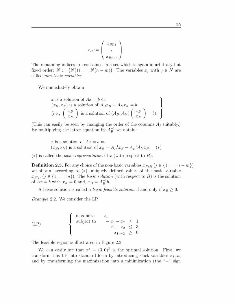
Example 2.2. We consider the LP
(LP)
maximize x1
subject to − x1 + x2 ≤ 1x1 + x2 ≤ 3x1, x2 ≥ 0.
The feasible region is illustrated in Figure 2.3.
We can easily see that x∗ = (3, 0)T is the optimal solution. First, wetransform this LP into standard form by introducing slack variables x3, x4
and by transforming the maximization into a minimization (the “−” sign

16CHAPTER 2. LINEAR PROGRAMMING: FOUNDATIONS AND
SIMPLEX METHOD
Figure 2.3: Feasible region.
in front of “min” can be dropped, but we must not forget this “−” wheninterpreting the final result). Hence we obtain
(LP)st
minimize − x1
subject to − x1 + x2 + x3 = 1x1 + x2 + x4 = 3x1, x2, x3, x4 ≥ 0,
i.e., c = (−1, 0, 0, 0)T , b = (1, 3)T and
A =
(−1 1 1 01 1 0 1
).
(i) For B = (B(1), B(2)) = (3, 4) we obtain the basic solution
xB =
(xB(1)
xB(2)
)=
(x3
x4
)= A−1
B b =
(1 00 1
)−1
b = b =
(13
),
xN =
(xN(1)
xN(2)
)=
(x1
x2
)= 0,
hence, x = (0, 0, 1, 3)T .
(ii) For B = (1, 2) we get by a proposition from linear algebra
AB =
(−1 11 1
)=⇒ A−1
B =1
2
(−1 11 1
),

17
therefore,
xB =
(xB(1)
xB(2)
)=
(x1
x2
)= A−1
B b =1
2
(−1 11 1
)(13
)=
(12
),
xN =
(xN(1)
xN(2)
)=
(x3
x4
)= 0,
hence, x = (1, 2, 0, 0)T .
(iii) For B = (4, 1) we get (exercise)
xB =
(x4
x1
)= A−1
B b =
(0 −11 1
)−1(13
)=
(4−1
),
xN =
(x2
x3
)= 0,
hence, x = (−1, 0, 0, 4)T .
Evaluation: In the cases (i), (ii), the basic solutions correspond to cornerpoints of P, namely, (i): x corresponds to the corner point (0, 0), and (ii): xcorresponds to the corner point (1, 2). Since xB ≥ 0 in both cases, (i) and(ii) yield basic feasible solutions.
In the case (iii) however, xB ≥ 0 is not satisfied. So, (xB, xN) is a basicsolution which is not feasible. In Figure 2.3, it can be easily seen that thecorresponding point (x1, x2) = (−1, 0) is not contained in P.
Now, we consider a basic feasible solution (xB, xN ) and use the basicrepresentation with respect to B to derive an optimality criterion. First, wepartition the coefficients of c into
cB := (cB(1), . . . , cB(m))T and
cN := (cN(1), . . . , cN(n−m))T .
Then, the objective value cTx can be written as

18CHAPTER 2. LINEAR PROGRAMMING: FOUNDATIONS AND
SIMPLEX METHOD
cTx = cTBxB + cTNxN
= cTB(A−1
B b− A−1B ANxN
)+ cTNxN
= cTBA−1B b+
(cTN − cTBA
−1B AN
)xN .
In the current basic feasible solution we have that xN = 0 and, therefore, itsobjective value is
cTBxB = cTBA−1B b.
For all other solutions the objective value differs from this value by(cTN −
cTBA−1B AN
)xN . If we increase the value of xN(j) = 0 to xN(j) = δ, δ > 0, then
the objective value is changed by
δ(cN(j) −
=:zN(j)︷ ︸︸ ︷cTBA
−1B︸ ︷︷ ︸
=:Π
AN(j)
).
Therefore, the objective value of the given basic feasible solution increases ifcN(j) − zN(j) > 0, and it decreases if cN(j) − zN(j) < 0. The values
cN(j) := cN(j) − zN(j),
called the reduced or relative costs of the non-basic variable xN(j), thus con-tain the information whether it is useful to increase the value of the non-basicvariable xN(j) from 0 to a value δ > 0. In particular, we obtain
Theorem 2.1 (Optimality Condition for Basic Feasible Solutions).If x is a basic feasible solution with respect to B and if
cN(j) = cN(j) − zN(j) = cN(j) − cTBA−1B AN(j) ≥ 0 ∀j ∈ 1, . . . , n−m ,
then x is an optimal solution of the LP
(LP)st
minimize cT
subject to Ax = bx ≥ 0.
As we have seen in Example 2.2, basic feasible solutions of Ax = b cor-respond to extreme points of the feasible region Ax ≤ b. Here, A is derivedfrom A by deleting those columns of A which correspond to a unit matrix,

19
and x are the components of x which correspond to the columns of A. Ac-cording to the idea mentioned at the beginning of this chapter, we will moveto a new basic feasible solution if the optimality condition is not satisfied forthe current basic feasible solution.
Example 2.3 (Continuation of Example 2.2). We apply our optimality testto two basic feasible solutions of Example 2.2:
(a) B = (1, 2): In (ii) we computed that
A−1B =
1
2
(−1 11 1
).
Thus, we obtain:
zN(1) =(cB(1), cB(2)
)A−1
B AN(1)
= (c1, c2)A−1B A3
= (−1, 0)12
(−1 11 1
)(10
)
= 12(1,−1)
(10
)
= 12
(i.e., Π = 12(1,−1)), N(1) = 3
=⇒ cN(1) = c3 − z3 = 0 − 12< 0.
So, the optimality condition is violated. Note that, using Theorem 2.1one cannot conclude that the corresponding basic feasible solution isnot optimal, since our theorem gives only a sufficient optimality condi-tion.
(b) B = (1, 3):
AB =
(−1 11 0
)=⇒ A−1
B =
(0 11 1
).
We check the optimality condition by computing c := cN − zN withzT
N := cTBA−1B AN , and check whether cN ≥ 0.

20CHAPTER 2. LINEAR PROGRAMMING: FOUNDATIONS AND
SIMPLEX METHOD
zTN = cTBA
−1B AN
= (c1, c3)A−1B (A1, A4)
= (−1, 0)
(0 11 1
)(1 01 1
)
= (−1, 0)
(1 12 1
)
= (−1,−1)=⇒ cN = (0, 0)T − (−1,−1)T = (1, 1)T ≥ 0.
Hence, the basic feasible solution
xB =
(x1
x3
)= A−1
B b =
(0 11 1
)(13
)=
(34
),
xN =
(x2
x4
)=
(00
)
corresponding to B is optimal. This basic feasible solution correspondsto the corner point
x∗ =
(x1
x2
)=
(30
),
which we have already identified in Example 2.2 as optimal using thegraphical-geometrical procedure.
In the following, we show how to obtain a new feasible solution if thecurrent one does not satisfy the optimality condition.
Suppose that cN(s) = cN(s) − zN(s) < 0 for some s ∈ N . Since
cTx = cTBA−1B b + (cTN − CT
BA−1B AN)xN
increasing xN(s) by one unit will decrease cTx by cN(s). Since our goal is tominimize the objective function cTx, we want to increase xN(s) by as manyunits as possible.
How large can xN(s) be chosen? This question is answered by the basicrepresentation (∗) and the requirement xB ≥ 0. If we keep xN(j), j 6= s,equal to 0 and increase xN(s) from 0 to δ ≥ 0, then we obtain for the resultingsolution of Ax = b

21
xB = A−1B b− A−1
B AN(s)δ.
Denoting the ith component of A−1B b and A−1
B AN(s) by bi and aiN(s), respec-tively, we have to choose δ such that
xB(i) = bi − aiN(s)δ ≥ 0. (⊗)
In order to choose δ as large as possible, we thus compute δ as
δ = xN(s) := min
bi
aiN(s)
∣∣ aiN(s) > 0
. (min ratio rule)
While computing δ with respect to the min ratio rule, two cases may occur:
Case 1: aiN(s) ≤ 0 ∀i ∈ 1, . . . , m.Then, δ can be chosen arbitrarily large without violating any of the nonneg-ativity of constraints. As a consequence, cTx can be made arbitrarily smalland the LP is unbounded. Thus we obtain:
Theorem 2.2 (Criterion on Unbounded LPs). If x is a basic feasiblesolution with respect to B and if
cN(s) < 0 and A−1B AN(s) ≤ 0
for some s ∈ N , then the LP
(LP)st
minimize cT
subject to Ax = bx ≥ 0
is unbounded.
Case 2: ∃i ∈ 1, . . . , m : aiN(s) > 0.In this case, the minimum in the computation of xN(s) by the min ratio rule
is attained. Suppose that we get δ = xN(s) =br
arN(s)
. (If the index r is not
uniquely determined, then we choose any of the indices such thatbr
arN(s)
= δ.)
According to (⊗) and the min ratio rule, the new solution is

22CHAPTER 2. LINEAR PROGRAMMING: FOUNDATIONS AND
SIMPLEX METHOD
xN(s) =br
arN(s)
, xN(j) = 0 ∀j 6= s,
xB(i) = bi − aiN(s)xN(s) = bi − aiN(s)br
arN(s)
∀i.
In particular, xB(r) = 0. It is easy to check that
B′ =(B′(1), . . . , B′(r − 1), B′(r), B′(r + 1), . . . , B′(m)
)
with
B′(i) :=
B(i) if i 6= rN(s) if i = r
defines a new basis for A (argument: arN(s) 6= 0). Thus, the computation ofxN(s) has induced a basis change. The variable xB(r) has left the basis, andxN(s) has entered the basis. The new index set of non-basic variables is
N ′ =(N ′(1), . . . , N ′(s− 1), N ′(s), N ′(s+ 1), . . . , N ′(n−m)
)
with
N ′(j) :=
N(j) if j 6= sB(r) if j = s.
Our basis change is indicated by Figure 2.4.
Figure 2.4: Basis change.
Example 2.4 (Continuation of Example 2.3). In (a), we saw that the opti-mality condition is violated for B = (1, 2). Since c3 < 0, we want to letxN(1) = x3 enter into the basis. We compute (cf. Example 2.3):
23
(a1N(1)
a2N(1)
)= A−1
B AN(1) =1
2
(−1 11 1
)(10
)=
1
2
(−11
),
b =
(b1b2
)= A−1
B b =1
2
(−1 11 1
)(13
)=
(12
)
=⇒ xN(1) = x3 =b2
a2N(1)
= 4.
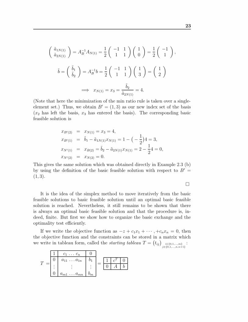
(Note that here the minimization of the min ratio rule is taken over a single-element set.) Thus, we obtain B ′ = (1, 3) as our new index set of the basis(x2 has left the basis, x3 has entered the basis). The corresponding basicfeasible solution is
xB′(2) = xN(1) = x3 = 4,
xB′(1) = b1 − a1N(1)xN(1) = 1 −(− 1
2
)4 = 3,
xN ′(1) = xB(2) = b2 − a2N(1)xN(1) = 2 − 1
24 = 0,
xN ′(2) = xN(2) = 0.
This gives the same solution which was obtained directly in Example 2.3 (b)by using the definition of the basic feasible solution with respect to B ′ =(1, 3).
It is the idea of the simplex method to move iteratively from the basicfeasible solutions to basic feasible solution until an optimal basic feasiblesolution is reached. Nevertheless, it still remains to be shown that thereis always an optimal basic feasible solution and that the procedure is, in-deed, finite. But first we show how to organize the basic exchange and theoptimality test efficiently.
If we write the objective function as −z + c1x1 + · · · ,+cnxn = 0, thenthe objective function and the constraints can be stored in a matrix whichwe write in tableau form, called the starting tableau T =
(tij)
i∈0,1,...,mj∈0,1,...,n,n+1
:
T =
1 c1 . . . cn 00 a11 . . . a1n b1...
......
0 am1 . . . amn bm
=1 cT 00 A b

24CHAPTER 2. LINEAR PROGRAMMING: FOUNDATIONS AND
SIMPLEX METHOD
Here, T represents a system of linear equations with m + 1 equations.The (n + 1)-st column contains the information about the right-hand sidesof the equations. If B is a basis, then we denote by TB the nonsingular(m+ 1) × (m+ 1) matrix
TB :=
(1 cTB0 AB
).
It is easy to verify that
T−1B :=
(1 −cTBA−1
B
0 A−1B
),
T−1B T =
(1 cT − cTBA
−1B A −cTBA−1
B b0 A−1
B A A−1B b
)=: T (B).
We call T (B) the simplex tableau associated with the basis B. Since T −1B
is nonsingular, T (B) represents the same system of linear equations as thestarting tableau T . The entries of T (B) can be interpreted as follows:
(i) The first column is always the first standard vector ET1 . It emphasizes
the character of the 0th row as an equation. Later on, we will omit thiscolumn.
(ii) For j = B(i) we have:
A−1B Aj = ET
i (being a column).
Furthermore,
cj − cTBA−1B Aj = cj − cj = 0 then
T (B) contains in the column corresponding to the ith basic variablexB(i) the value 0 in row 0 and, then, the ith unit vector ET
i with mcomponents.
(iii) For j = N(i) we have:
A−1B Aj = (a1j , ..., amj)
T .
25
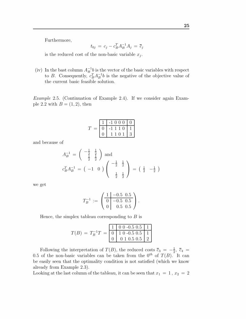
Furthermore,t0j = cj − cTBA
−1B Aj = cj
is the reduced cost of the non-basic variable xj.
(iv) In the bast column A−1B b is the vector of the basic variables with respect
to B. Consequently, cTBA−1B b is the negative of the objective value of
the current basic feasible solution.
Example 2.5. (Continuation of Example 2.4). If we consider again Exam-ple 2.2 with B = (1, 2), then
T =1 -1 0 0 0 00 -1 1 1 0 10 1 1 0 1 3
and because of
A−1B =
(−1
212
12
12
)and
cTBA−1B =
(−1 0
)
−12
12
12
12
=
(12
−12
)
we get
T−1B :=
1 −0.5 0.50 −0.5 0.50 0.5 0.5
.
Hence, the simplex tableau corresponding to B is
T (B) = T−1B T =
1 0 0 -0.5 0.5 10 1 0 -0.5 0.5 10 0 1 0.5 0.5 2
Following the interpretation of T (B), the reduced costs c3 = −12, c4 =
0.5 of the non-basic variables can be taken from the 0th of T (B). It canbe easily seen that the optimality condition is not satisfied (which we knowalready from Example 2.3).Looking at the last column of the tableau, it can be seen that x1 = 1 , x2 = 2

26CHAPTER 2. LINEAR PROGRAMMING: FOUNDATIONS AND
SIMPLEX METHOD
are the values of the basic variables in the basic feasible solution, yielding anobjective value of −t0n+1 = −1.
If ∃j ∈ 1, ..., n : t0j < 0, then we try to more the non-basic variablexnj into the basis. Since the entries of the tableau are
t1j = a1j , ..., tmj = amj ,
andt1n+1 = b1, ..., tmn+1 = bm,
we can perform the min ratio test using the simplex tableau in a very simpleway:
δ = xj := min
ti n+1
ti j
∣∣∣ ti j > 0
.
Thus, an unbounded objective function can be recognized by the fact thatthe column corresponding to one of the non - basic variables xj with t0j < 0contains only entries ≤ 0 (cf. Theorem 2.2).
If δ = tr n+1
tr j, a pivot operation is carried out with the element tr j > 0,
i.e., we transform the jth column of T (B) into the jth standard (column)vector ET
j using only elementary row operations. The resulting tableau isthe simplex tableau T (B ′) with respect to the new basis B ′.
Example 2.6. (Continuation of Example 2.5). Let us come back to Exam-ple 2.5:Since t03 = −1
2, we try to move x3 into the basis. The min ratio rule yields
δ = x3 =t25t23
=2
0.5= 4.
Hence, we pivot the last tableau (see above) with the element t23 = 0.5.
T (B) =1 0 0 -0.5 0.5 10 1 0 -0.5 0.5 10 0 1 0.5 0.5 2
∼
1 0 1 0 1 30 1 1 0 1 30 0 2 1 1 4
= T (B′).

27
In T (B′), all reduced cost values (= t0j , j ∈ 1, ..., m are ≥ 0: Thecorresponding basic solution with
x1 = 3, x3 = 4 , x2 = x4 = 0
is optimal.
If t0j ≥ 0, ∀j ∈ 1, ..., n and tin+1 ≥ 0, ∀i ∈ 1, ..., m , then T (B) iscalled an optimal (simplex) tableau. We summarize:
Algorithm (Simplex Method for the Solution of LPs of the type min cTx :Ax = b, x ≥ 0)
(Input) Basic feasible solution (xB, xN ) with respect to basis B.(1) Compute the simples tableau T (B).(2) If t0j ≥ 0 ∀j = 1, . . . , n,
(STOP) (xB, xN ) with xB(i) = tin+1 (i = 1, . . . , m) xN = 0and with the objective value−t0n+1 is an optimal solution of LP.
(3) Choose j with t0j < 0.(4) If tij ≤ 0 ∀i = 1, . . . , m (STOP) The LP is unbounded.(5) Determine r ∈ 1, . . . , m with
trn+1
tij= min
trn+1
tij
∣∣ tij > 0
and pivot with trj.Goto (2).
For the well-definiteness of (1) we state:
Theorem 2.3 (Fundamental Theorem of LPs). Suppose that an LP
(LP)st
minimize cTxsubject to Ax = b
x ≥ 0
is given and that P := x ∈ Rn |Ax = b, x ≥ 0 6= ∅ . Then, there exists
a basic feasible solution.
Proof. cf., e.g., Hamacher, Klamroth, (2000).

28CHAPTER 2. LINEAR PROGRAMMING: FOUNDATIONS AND
SIMPLEX METHOD
We conclude our first chapter by an example:
Example 2.7. Solve the LP
(LP)
maximize 3x1 + x2
subject to −x1 + x2 ≤ 1x1 − x2 ≤ 1
x2 ≤ 2x1 , x2 ≥ 0
by the Simplex Method.
Solution:First we transform LP into standard form:
(LP)st
(-) minimize −3x1 − x2
subject to −x1 + x2 +x3 = 1x1 − x2 + x4 = 1
x2 + x5 = 2x1 , x2 , x3 , x4 , x5 ≥ 0
(The ”-” in front of ”min” will be omitted in the following.) As a conse-quence, the objective function value of the current basic feasible solution is−(−t06) = t06 in the following tableaus (and not −t06).
A basic feasible starting solution is given by B = (3, 4, 5), i.e., the slackvariables are the basic variables. The first simplex tableau is therefore (with-out the Oth column):
T (B) =
-3 -1 0 0 0 0-1 1 1 0 0 11 -1 0 1 0 10 1 0 0 1 2
While applying the Simplex Method, we indicate the pivot column (i.e.,the column corresponding to a non-basic variable xj with t0j < 0) and thepivot row (i.e., the row r determined by (5)) by representing the pivot ele-ment in boldface.

29
T (B) ∼0 -4 0 3 0 30 0 1 1 0 21 -1 0 1 0 10 1 0 0 1 2
∼0 0 0 3 4 110 0 1 1 0 21 0 0 1 1 30 1 0 0 1 2
optimal tableau
(STOP) (xB , xN) with
xB =
x3
x1
x2
=
232
and xN =
(x4
x5
)=
(00
),
hence,
x∗ :=
x1
x2
x3
x4
x5
=
23200
is optimal with objective value 11.
With our next chapter we remain in the field of LP, but follow a basicallydifferent approach in solving the linear program.

30CHAPTER 2. LINEAR PROGRAMMING: FOUNDATIONS AND
SIMPLEX METHOD

Chapter 3
Linear Programming:Interior-Point Methods
3.1 Introduction
In the 80s of 20th century, it was discovered that many large linear pro-grams could be solved efficiently by formulating them as nonlinear problemsand solving them with various modifications of nonlinear algorithms such asNewton’s method. One characteristic of these methods was that they re-quired to satisfy inequality constraints strictly. So, they soon became calledinterior-point methods. By the early 90s of last century, one class —so-calledprimal-dual methods— had distinguished itself as the most efficient practicalapproach and proved to be a strong competitor to the simplex method onlarge problems. These methods are the focus of this chapter.
The simplex method can be quite inefficient on certain problems: Thetime required to solve a linear program may be exponential in the problem’ssize, as measured by the number of unknowns and the amount of storageneeded for the problem data. In practice, the simplex method is much moreefficient than this bound would suggest, but its poor worst-case complexitymotivated the development of new algorithms with better guaranteed perfor-mance. Among them is the ellipsoid method proposed by Khachiyan (1979),which finds a solution in time that is at worst polynomial in the problem size.Unfortunately, this method approaches its worst-case bound on all problemsas is not competitive with the simplex method. Karmarkar (1984) announceda projective algorithm which also has polynomial complexity, but it camewith the added inducement of a good practical behaviour. The initial claimsof excellent performance on large linear programs were never fully borne out,

32CHAPTER 3. LINEAR PROGRAMMING: INTERIOR-POINT
METHODS
but the announcement prompted a great deal of research activity and a widearray of methods described by such labels as “affine-scaling ”, “logarithmic-barrier”, “potential-reduction”, “path-following”, “primal-dual”, and “infea-sible interior point”. Many of the approaches can be motivated and describedindependently of the earlier ones of Karmarkar or of so-called log-barrier, etc..
Interior-point methods share common features that distinguish them fromthe simplex method. Each interior-point iteration is expensive to computeand can make a significant progress towards the solution, while the simplexmethod usually requires a large number of inexpensive iterations. The sim-plex method works its way around the boundary of the feasible polytope,testing a sequence of vertices in turn until it finds the optimal one. Interior-point methods approach the boundary of the feasible set in the limit. Theymay approach the solution either from the interior or from the exterior of thefeasible region, but they never actually lie on the boundary of this region.
3.2 Primal-Dual Methods
Outline: Let our LP be given in standard form:
(LP)st
minimize cTxsubject to Ax = b
x ≥ 0;
cf. Chapter 2. The dual (linear) problem, LDP, is defined by
(DP)
maximize bTysubject to ATy + s = c,
s ≥ 0,
where y ∈ Rm (dual variable) and s ∈ R
n (slack variable). “Primal-dual”solutions of (LP)st, (DP) fulfill the (first-order) necessary optimality condi-tions from general optimization theory which are called Karush-Kuhn-Tuckerconditions (cf. Section 1.1). We state them here as follows (exercise):
(NOC)
ATy + s = c,Ax = b,xjsj = 0 ∀j ∈ 1, 2, . . . , n ,
(x, s) ≥ 0.1
1Please consider the following Lagrange function: L(x, y, s) := cT x−yT (Ax− b)−sTx.
The condition (x, s) ≥ 0 just means nonnegativity of all xj , sj .

3.2. PRIMAL-DUAL METHODS 33
Primal-dual methods find solutions (x∗, y∗, s∗) of (NOC) by applying vari-ants of Newton’s method to the three groups of equalities, and modifyingthe search directions and step lengths so that the inequalities (x, s) ≥ 0are satisfied strictly at every iteration. The equations in (NOC) are onlymildly nonlinear and so are not difficult to solve by themselves. However, theproblem becomes more difficult when we add the nonnegativity requirement(x, s) ≥ 0. The nonnegativity condition is the source of all the complicationsin the design and analysis of interior-point methods.
To derive primal-dual interior-point methods, we restate (NOC) in aslightly different form by a mapping F : R
2n+m −→ R2n+m:
(NOC)
F (x, y, s) :=
AT y + s− cAx− bXS 1
!
= 0,
(x, s) ≥ 0,
where
X := diag(x1, x2, . . . , xn),
S := diag(s1, s2, . . . , sn), and
1 := (1, 1, . . . , 1)T .
Primal-dual methods generate iterates (xk, yk, sk) that satisfy the bounds(x, s) ≥ 0 strictly, i.e., xk > 0 and sk > 0. By respecting these bounds,the interior-point methods avoid spurious solutions, i.e., points that sat-isfy F (x, y, s) = 0 but not (x, s) ≥ 0. Spurious solutions abound and donot provide useful information about solutions of (LP)st and (DP). So, itis reasonable to exclude them altogether from the region of search. Manyinterior-point methods actually require (xk, yk, sk) to be strictly feasible, i.e.,to satisfy the linear equality constraints for the primal and dual problems.We put
M :=(x, y, s)
∣∣ Ax = b, ATy + s = c, (x, s) ≥ 0,
M0 :=(x, y, s)
∣∣ Ax = b, AT y + s = c, (x, s) > 0
;

34CHAPTER 3. LINEAR PROGRAMMING: INTERIOR-POINT
METHODS
so, M0 is some relative interior of M. Herewith, the strict feasibility condi-tion can be written concisely as
(SF) (xk, yk, sk) ∈ M0 ∀k ∈ N0.
Primal-dual interior point methods consist of both
(a) a procedure for determining the step,
(b) a measure of desirability of each point in search space.
The search direction procedure has its origins in Newton’s method, here,
applied to nonlinear equations F!= 0 in (NOC). Newton’s method forms a
linear model for F around the current point and obtains the search direction(∆x,∆y,∆s) by solving the following system of linear equations (exercise):
DF (x, y, s)
∆x∆y∆s
= −F (x, y, s).
If (x, y, s) ∈ M0 (strict feasibility!), then the Newton step equations become
(ASD)sf
0 AT IA 0 0S 0 X
∆x∆y∆s
=
00
−XS 1
.
Usually, a full step along this direction is not permissible, since it wouldviolate the bound (x.s) ≥ 0. To avoid this difficulty, we perform a linesearch along the Newton direction so that the new iterate is
(x, y, s) + α(∆x,∆y,∆s)
for some line search parameter α ∈ (0, 1]. Unfortunately, we often can takeonly a small step along the direction (i.e., α << 1) before violating thecondition (x, s) > 0. Hence, the pure Newton iteration (ASD), which isknown as the affine scaling direction, often does not allow us to make muchprogress towards a solution. Primal-dual methods modify the basic Newtonprocedure in two ways:

3.2. PRIMAL-DUAL METHODS 35
(i) They bias the search direction towards the interior of the “nonnegativeorthant” (x, s) ≥ 0, so that we can move further along the directionbefore one of the components of (x, s) becomes negative.
(ii) They keep the components of (x, s) from moving “too close” to theboundary of the nonnegative orthant.
We consider these modifications in turn.
The Central Path (embedding our framework): The central path Cconsists of strictly feasible points (xτ , yτ , sτ ) ∈ C parametrized by a scalarτ > 0, where each point solves the following system:
(NOC)τsf
ATy + s = c,Ax = b,xjsj = τ ∀j ∈ 1, 2, . . . , n ,
(x, s) > 0.
From (NOC)τsf we can define the central path as C :=
(xτ , yτ , sτ )
∣∣ τ > 0.
In fact, it can be shown that (xτ , yτ , sτ ) is uniquely defined for each τ > 0if and only if M0 6= ∅. A plot of C for a typical problem, projected into thespace of primal variables x, is shown in Figure 3.1:
Figure 3.1: Central path, projected into x-space, showing a typical neigh-bourhood N .

36CHAPTER 3. LINEAR PROGRAMMING: INTERIOR-POINT
METHODS
Another way of defining C is to use our mapping F (see (NOC)) and write
(NOC)τsf F (xτ , yτ , sτ ) =
00τ1
, (xτ , sτ ) > 0.
The equations (NOC)τsf approximate the ones in (NOC) more and more as
τ → 0. If C converges to anything as τ → 0, then it must converge to aprimal-dual solution of the linear problem. The central path thus guides usto a solution along a route that steers clear of spurious solutions by keeping allx- and s- components strictly positive and decreasing the pairwise productsxjsj to 0 at roughly the same rate.
Primal-dual algorithms take Newton steps towards points on C for whichτ > 0, rather that pure Newton steps for F . Since these steps are biasedtowards the interior of the nonnegative orthant (x, s) ≥ 0, it usually is pos-sible to take longer steps along them than along the pure Newton steps forF , before violating the positivity condition.
To describe the biased search direction, we introduce a centering param-eter σ ∈ [0, 1] and a duality measure µ defined by the average
µ :=1
n
n∑
j=1
xjsj =1
nxT s.
By writing τ := σµ and applying Newton’s method to (NOC)τsf , we obtain
(ASD)σµsf
0 AT IA 0 0S 0 X
∆x∆y∆s
=
00
−XS 1 + σµ1
.
The step (∆x,∆y,∆s) is a Newton step towards the point (xσµ, yσµ, sσµ) ∈ C,at which the pairwise products xjsj are equals to σµ.
If σ = 1, then (ASD)τsf defines a centering direction, a Newton step
towards the point (xµ, yµ, sµ) ∈ C, at which xjsj = µ for all j. Centeringdirections are usually biased strongly towards the interior of the nonnegativeorthant and make little progress in reducing the duality measure µ. Bymoving closer to C, however, they set the scene for substantial progress onthe next iteration.
If σ = 0, then we get the standard Newton step (ASD)sf . many algo-rithms use intermediate values of σ ∈ (0, 1) to trade off between the twin

3.2. PRIMAL-DUAL METHODS 37
goals of reducing µ and improving centrality.
A Primal-Dual Framework: With our concepts from above, we candefine a general framework for primal-dual algorithms:
Framework IPM1 Primal-Dual
Given (x0, y0, s0) ∈ M0
for k = 0, 1, 2, . . .Solve
(ASD)σkµk
sf
0 AT IA 0 0Sk 0 Xk
∆xk
∆yk
∆sk
=
00
−XkSk1 + σkµk1
,
where σk ∈ [0, 1] and µk = (xk)T sk/n;Set
(xk+1, yk+1, sk+1) = (xk, yk, sk) + αk(∆xk,∆yk,∆sk),
choosing αk such that (xk+1, sk+1) > 0.end(for).
The choices of centering parameter σk and step length αk are crucial tothe performance of the method. Techniques for controlling these parametersgive rise to a wide variety of methods with varying theoretical properties.
So far, we have assumed that the starting point (x0, y0, s0) is strictlyfeasible and, in particular, that it satisfies the linear equations Ax0 = b,ATy0+s0 = c. All subsequent iterates also respect these constraints, becauseof the zero right-hand-side terms in (ASD)σkµk
sf . However, for most problems,a strictly feasible starting point is difficult to find! Infeasible-interior-pointmethods require only that the components of x0 and s0 be strictly positive.The search direction needs to be modified so that it improves feasibility aswell as centrality at each iteration, but this requirement entails only a slightchange to the step equation (ASD)σµ
sf .
If we define the residuals for the two linear equations as
rb := Ax− b, rc := ATy + s− c,
then the modified step equation is
(ASD)σµinf
0 AT IA 0 0S 0 X
∆x∆y∆s
=
−rc
−rb
−XS 1 + σµ1
.
38CHAPTER 3. LINEAR PROGRAMMING: INTERIOR-POINT
METHODS
The search direction is still a Newton step towards the point (xσµ, yσµ, sσµ) ∈C. It tries to correct all the infeasibility in the equality constraints in a singlestep. If a full step is taken at any iteration (i.e., ∃k : αk = 1), the residualsrb and rc become 0, and all subsequent iterates remain strictly feasible.
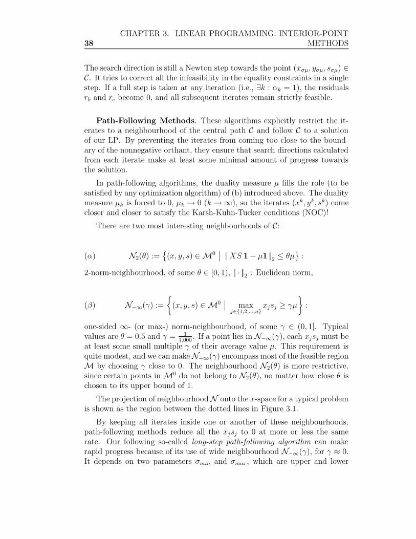
Path-Following Methods: These algorithms explicitly restrict the it-erates to a neighbourhood of the central path C and follow C to a solutionof our LP. By preventing the iterates from coming too close to the bound-ary of the nonnegative orthant, they ensure that search directions calculatedfrom each iterate make at least some minimal amount of progress towardsthe solution.
In path-following algorithms, the duality measure µ fills the role (to besatisfied by any optimization algorithm) of (b) introduced above. The dualitymeasure µk is forced to 0, µk → 0 (k → ∞), so the iterates (xk, yk, sk) comecloser and closer to satisfy the Karsh-Kuhn-Tucker conditions (NOC)!
There are two most interesting neighbourhoods of C:
(α) N2(θ) :=(x, y, s) ∈ M0
∣∣ ||XS 1 − µ1 ||2 ≤ θµ
:
2-norm-neighbourhood, of some θ ∈ [0, 1), || · ||2 : Euclidean norm,
(β) N−∞(γ) :=
(x, y, s) ∈ M0
∣∣ maxj∈1,2,...,n
xjsj ≥ γµ
:
one-sided ∞- (or max-) norm-neighbourhood, of some γ ∈ (0, 1]. Typicalvalues are θ = 0.5 and γ = 1
1,000. If a point lies in N−∞(γ), each xjsj must be
at least some small multiple γ of their average value µ. This requirement isquite modest, and we can make N−∞(γ) encompass most of the feasible regionM by choosing γ close to 0. The neighbourhood N2(θ) is more restrictive,since certain points in M0 do not belong to N2(θ), no matter how close θ ischosen to its upper bound of 1.
The projection of neighbourhood N onto the x-space for a typical problemis shown as the region between the dotted lines in Figure 3.1.
By keeping all iterates inside one or another of these neighbourhoods,path-following methods reduce all the xjsj to 0 at more or less the samerate. Our following so-called long-step path-following algorithm can makerapid progress because of its use of wide neighbourhood N−∞(γ), for γ ≈ 0.It depends on two parameters σmin and σmax, which are upper and lower

3.2. PRIMAL-DUAL METHODS 39
bounds on the centering parameter σk. As usual, the search direction isobtained by solving (ASD)σkµk
sf , and we choose the step length αk to be aslarge as possible, subject to staying inside N−∞(γ).
Here and later on, we use the notation
(xk(α), yk(α), sk(α)) := (xk, yk, sk) + α(∆xk,∆yk,∆sk),µk(α) := 1
nxk(α)sk(α)
(cf. our corresponding definitions from above).
Algorithm IPM2 (Long-Step Path-Following)
Given γ, σmin, σmax with γ ∈ (0, 1), 0 < σmin < σmax < 1,and (x0, y0, s0) ∈ N−∞(γ);
for k = 0, 1, 2, . . .Choose σk ∈ [σmin, σmax];Solve (ASD)σkµk
sf to obtain (∆xk,∆yk,∆sk);
Choose αk as the largest value of α in [0, 1] such that
(xk(α), yk(α), sk(α)) ∈ N−∞(γ);
Set (xk+1, yk+1, sk+1) = (xk(αk), yk(αk), s
k(αk));end(for).
The typical behaviour of our algorithm is illustrated in Figure 3.2 for thecase of n = 2. The horizontal and vertical axes in this figure represent thepairwise product x1s1 and x2s2; so the central path C is the line emanatingfrom the origin at an angle of 45o. (Here, a point at the origin is a primal-dual solution if it also satisfies the feasibility conditions from (NOC) differentfrom xjsj = 0.) In the usual geometry of Figure 3.2, the search directions(∆xk,∆yk,∆sk) transform to curves rather than lines. As Figure 3.2 shows,the bound σmin ensures that each search direction stands out by movingaway from the boundary of N−∞(γ) and into the relative interior of thisneighbourhood. That is, small steps along the search direction improve thecentrality.
Larger values of α take us outside the neighbourhood again, since the errorin approximating the nonlinear system (NOC)τ
sf by the linear step equations(ASD)σµ
sf becomes more pronounced as α increases. Still, we are guaranteedthat a certain minimum step can be taken before we reach the boundary ofN−∞(γ). A complete analysis of Algorithm IPM2 can be found in Nocedal,

40CHAPTER 3. LINEAR PROGRAMMING: INTERIOR-POINT
METHODS
Figure 3.2: Iterates of Algorithm IPM2 plotted in (x, s)-space.
Wright (1999). It shows that the primal-dual methods can be understoodwithout recourse to profound mathematics. This algorithm is fairly efficientin practice, but with a few more changes it becames the basis of a trulycompetitive method.
An infeasible-interior-point variant of Algorithm IPM2 can be constructedby generalizing the definition of N−∞(γ) to allow violation of the feasibilityconditions. In this extended neighbourhood, the residual norms || rb || and|| rc || are bounded by a constant multiple of the duality measure µ. Bysqueezing µ to 0, we also force rb and rc to 0, so that the iterates approachcomplementarity and feasibility simultaneously.
3.3 A Practical Primal-Dual Algorithm
Most existing interior-point codes are based on a predictor-corrector algo-rithm proposed by Mehrotra (1992). The two key features of this algorithmare:
(I) addition of a corrector step to the search direction of Framework IPM1,

3.3. A PRACTICAL PRIMAL-DUAL ALGORITHM 41
so that the algorithm more closely follows a trajectory to the primal-dual solution set;
(II) adaptive choice of the centring parameter σ.
In (I), we shift the central path C so that it starts at our current iterate(x, y, s) and ends at the set Ω of solution points. Let us denote this modifiedtrajectory by H and parametrize it by the parameter τ ∈ [0, 1], so that
H =(x(τ), y(τ), s(τ))
∣∣ τ ∈ [0, 1),
with x(0), y(0), s(0)) = (x, y, s) and
limτ→1−
(x(τ), y(τ), s(τ)) ∈ Ω
(see Figure 3.3).
Figure 3.3: Central path C, and a trajectory H from the current (noncentral)point (x, y, s) to the solution set Ω.
Algorithms from Framework IPM1 are first-order methods, in that theyfind the tangent to a trajectory like H and perform line search along it.This tangent is knows as the predictor step. Mehrotra’s algorithm takes thenext step of calculating the curvature of H at the current point, therebyobtaining a second-order approximation of this trajectory. The curvature isused to define the corrector step. It can be obtained at a low marginal cost,since it reuses the matrix factors from the calculation of the predictor step.

42CHAPTER 3. LINEAR PROGRAMMING: INTERIOR-POINT
METHODS
In (II), we chose the centering parameter σ adaptively, in contrast to algo-rithms from Framework IPM1, which assign a value to σk prior to calculatingthe search direction. At each iteration, Mehrotra’s algorithm first calculatesthe affine-scaling direction (the predictor step) and assesses its usefulness asa search direction. If this direction yields a large reduction in µ withoutviolating the positivity condition (x, s) > 0, then the algorithm concludesthat little centering is needed. So, it chooses σ close to zero and calculates acentered search direction with this small value. If the affine-scaling directionis not so productive the algorithm enforces a larger amount of centering bychoosing a value of σ closer to 1.
The algorithm thus combines three steps to form the research direction:a predictor step which allows us to determine the centering parameter σk, acorrector step using second-order information of the path H leading towardsthe solution, and centering step in which the chosen value of σk is substitutedin (ASD)σµ
inf . Hereby, the computation of the centered direction and thecorrector step can be combined, so that adaptive centering does not addfurther to the cost of each iteration.
For the computation of the search direction (∆x,∆y,∆s) we proceed asfollows:
First, we calculate the predictor step (∆xaff ,∆yaff ,∆saff ) by settingσ = 0 in (ASD)σµ
inf , i.e.,
(ASD)0,affinf
0 AT IA 0 0S 0 X
∆xaff
∆yaff
∆saff
=
−rc
−rb
−XS 1
.
To measure the effectiveness of this direction, we find αpriaff and αdual
aff to thelargest length that can be taken along this direction before violating thenonnegativity conditions (x, s) ≥ 0, and an upper bound of 1:
αpriaff := min
1, min
j:∆xaffj <0
− xj
∆xaffj
,
αdualaff := min
1, min
j:∆saffj <0
− sj
∆saffj
.
Furthermore, we define µaff to be the value of µ that would be obtained bya full step to the boundary, i.e.,

3.3. A PRACTICAL PRIMAL-DUAL ALGORITHM 43
µaff :=1
n
(x + αpri
aff∆xaff) (s + αpri
aff∆saff),
and set the damping parameter σ to be
σ :=
(µaff
µ
)3
.
When good progress is made along the predictor direction, then we haveµaff << µ, so this σ is small; and conversely.
The corrector step is obtained by replacing the right-hand-side of (ASD)0,affinf
by (0, 0,−∆Xaff ,∆Saff1), while the centering step requires a right-hand-side of (0, 0, σµ1). So we can obtain the complete Mehrotra step, whichincludes the predictor, corrector and centering step components, by addingthe right-hand-sides of these three components and solving the following sys-tem:
(⊕)
0 AT IA 0 0S 0 X
∆x∆y∆s
=
−rc
−rb
−XS 1 − ∆Xaff∆Saff1 + σµ1
.
We calculate the maximum steps that can be taken along these directionsbefore violating the nonnegativity condition (x, s) > 0 by formulae similarto the ones for αpri
aff and αdualaff ; namely,
αprimax := min
1, min
j:∆xj<0− xk
j
∆xj
,
αdualmax := min
1, min
j:∆sj<0− sk
j
∆sj
,
and then choose the primal and dual step lengths as follows
αprik := min
1, ηαpri
max
,
αdualk := min
1, ηαdual
max
,
where η ∈ [0.9, 1.0) is chosen so that η → 1 near the solution, to acceleratethe asymptotic convergence.

44CHAPTER 3. LINEAR PROGRAMMING: INTERIOR-POINT
METHODS
We summarize this discussion by specifying Mehrotra’s algorithm in theusual format.
Algorithm IPM3 (Mehrotra Predictor-Corrector Algorithm)
Given (x0, y0, s0) with (x0, s0) > 0;for k = 0, 1, . . .
Set (x, y, s) = (xk, yk, sk) and
solve (ASD)0,affinf for (∆xaff ,∆yaff ,∆saff );
Calculate αpriaff , α
dualaff , and µaff ;
Set centering parameter to σ = (µaff/µ)3;Solve (⊕) for (∆x,∆y,∆s);
Calculate αprik and αdual
k ;Set
xk+1 = xk + αprik ∆x,
(yk+1, sk+1) = (yk, sk) + αdualk (∆y,∆s);
end(for).
It is important to note that no convergence theory is available for Mehro-tra’s algorithm in its previous form. In fact, there are examples for whichthe algorithm diverges. Simple safeguards could be incorporated into themethod to force it into the convergence framework of existing methods. How-ever, most programs do not implement these safeguards, because the goodpractical performance of Mehrotra’s algorithm makes them unnecessary.
For more information about primal-dual interior-point methods we referto Nocedal, Wright (1999) and to Nash, Sofer (1996).

Chapter 4
Nonlinear Programming:Feasible-Point Methods
In this chapter, we examine methods which solve constrained (nonlinear) op-timization problems by attempting to remain feasible at every iteration. Ifall the constraints are linear, maintaining feasibility is straightforward. Wediscuss this case first. When nonlinear constraints are present, then moreelaborate procedures are required. We discuss two such approaches: se-quential quadratic programming and reduced-gradient methods. Both theseapproaches generalize the techniques for linear constraints. Although theyare motivated by the idea of maintaining feasibility at every iteration, the donot always achieve this.
4.1 Linear Equality Constraints
The majority of methods for solving problems with linear equality constraintsare feasible-point methods: They start from a feasible point and move alongfeasible descent directions to consecutively better feasible points. There aretwo features making this approach particularly attractive:
(i) It is practically advantageous that all iterates are feasible. Even if thealgorithm fails to solve the problem to the desired accuracy, it mightstill provide a feasible solution that is usable.
(ii) By restricting movement to feasible directions, the equality-constrainedproblem is transformed to an unconstrained one in the null space of the

46CHAPTER 4. NONLINEAR PROGRAMMING: FEASIBLE-POINT
METHODS
constraints. This new problem may then be solved using unconstrainedminimization techniques.
Let us write our problem as follows:
(NLP)
minimize f(x)subject to Ax = b,
where f is twice-continuously differentiable: f ∈ C2, and A is anm×nmatrixof full row rank, where m ≤ n. As in the constrained case, the methods wedescribe are only guaranteed to find a stationary point of the problem. Inthe special case where f is convex, this point will be a global minimizer of f .
Let x be a feasible point, i.e., Ax = b. Since any other feasible point canbe reached from x by moving in a feasible direction, the solution to (NLP)can be written as x∗ = x+ p, where p solves the problem
minimize f(x+ p)subject to Ap = 0,
(Note: Ap = A(x∗ − x) = Ax∗ − Ax = b− b = 0).
Let Z denote an n × (n −m) basis matrix for the null-space (kernel) ofA. Then, p = Zv for some (n − m)-dimensional vector v. This problem isequivalent to the unconstrained problem
minimize ϕ(v) := f(x+ Zv).
So, we have reduced the problem of finding the best n-dimensional vector pto the unconstrained problem of finding the best (n−m)-dimensional vectorv.
Conceptually, it is possible to minimize the reduced function ϕ using anyof the unconstrained methods. In practice it is not necessary to provide anexplicit expression for ϕ(v). Instead, it is possible to work directly with theoriginal variable x, using
(∗) ∇ϕ(v) = ZT∇f(x), and
(∗∗) ∇2ϕ(v) = ZT∇2f(x)Z,

4.1. LINEAR EQUALITY CONSTRAINTS 47
where x = x + Zv. Let us shortly demonstrate this:
ϕ(v) = f(x+ Zv) = f(x) + vTZT∇f(x) +1
2vTZT∇2f(x)Zv + · · · .
Ideally, we would like to use the Newton direction; it is obtained by mini-mizing the quadratic approximation to ϕ(v) obtained from the Taylor series.Setting the gradient of the quadratic approximation to 0 gives the followinglinear system in v:
(ZT∇2f(x)Z
)v = −ZT∇f(x),
called the reduced Newton (or null-space) equation. Its solution is just
v = −(ZT∇2f(x)Z
)−1ZT∇f(x),
being an estimate of the best. In turn, it provides an estimate of the best p:
p = Zv = −Z(ZT∇2f(x)Z
)−1ZT∇f(x),
called the reduced Newton direction at x. Now, we can derive the equality-constrained analog of the classical Newton method. The method sets
xk+1 := xk + pk,
where pk = −Z(ZT∇2f(xk)Z
)−1ZT∇f(xk) is the reduced Newton direction
at xk. This is just the mathematical formulation of the method, and inpractice, explicit inverses are not normally computed. The method does notrequire that the reduced function be formed explicitly.
Example 4.1. We consider the problem:
(NLP)=
minimize f(x) = 12x2
1 − 12x2
3 + 4x1x2 + 3x1x3 − 2x2x3
subject to x1 − x2 − x3 = −1(i.e., A := (1,−1,−1), b = (−1)).
As a basis matrix for the null-space of A we choose
Z =
1 11 00 1
.

48CHAPTER 4. NONLINEAR PROGRAMMING: FEASIBLE-POINT
METHODS
The reduced gradient at x := (1, 1, 1)T , being the feasible point which weconsider, is
ZT∇f(x) =
(1 1 01 0 1
)
820
=
(108
),
and the reduced Hessian matrix at x is
ZT∇2f(x)Z =
(1 1 01 0 1
)
1 4 34 0 −23 −2 −1
1 11 00 1
=
(9 66 6
).
The reduced Newton equation yields
v =
(−2
3
−23
);
hence, the reduced Newton direction is
p = Zv =
−43
−23
−23
.
Since the objective function is quadratic and the reduced Hessian matrixis positive definite, a step length of α = 1 leads to the optimum x∗ =(−1
3, 1
3, 1
3
)T. At x∗, the reduced gradient is ZT∇f(x∗) = ZT (2,−2, 2)T = 0
as expected. The corresponding Lagrange multiplier is λ∗ = 2, because
∇f(x∗) = 2AT .
The reduced Newton direction is invariant with respect to the null-spacematrix Z: Any choice of the basis matrix Z will yield the same search di-rection p. Numerically, however, the choice of Z can have dramatic effect onthe computation.
The classical reduced Newton method has all the properties of the clas-sical Newton method. In particular, if the reduced Hessian matrix at thesolution is positive definite, and if the starting point is sufficiently close to

4.1. LINEAR EQUALITY CONSTRAINTS 49
the solution, then the iterates will converge quadratically. In the more gen-eral case, however, the method may diverge or fail. Then, some globalizationstrategy should be used.
If xk is not a local solution and if the reduced Hessian matrix is positivedefinite, then the reduced Newton direction is a descent direction, since
pT∇f(xk) = −∇f(xk)Z(ZT∇2f(xk)Z
)−1ZT∇f(xk),
< 0.
If the Hessian matrix is not positive definite, then the search directionmay not be a descent direction, and worse still, it may not be defined. Then,the modified factorizations can be applied to the reduced Hessian matrix toprovide a descent direction; see Nash, Sofer (1996).
Other compromises on Newton’s method may be made to obtain cheaperiterations. The simplest of all methods is of course the steepest-descentmethod. For the reduced function, this strategy gives the direction
v = −ZT∇f(xk)
in the reduced space, which yields the reduced steepest-descent direction
p = −ZZT∇f(xk)
in the original space. Here, Z may be any null-space matrix for A. However,the direction will vary with the particular choice of Z, unlike the reducedNewton direction!
Example 4.2. The reduced gradient at the initial point of Example 4.1 isZT∇f(x) = (10, 8)T ; hence, the reduced steepest-descent direction is p =−ZZT∇f(x) = (−18,−10,−8)T . Had we chosen
Z =
2 01 41 −4
as the null-space matrix for A, the reduced gradient would be ZT∇f(x) =
ZT (8, 2, 0)T = (18, 8)T , and the reduced steepest-descent direction would be
p = −ZZT∇f(x) = (−36,−50, 14)T .
The reduced steepest-descent method has the same properties as that ofits classical unconstrained counterpart. The iterations are cheap, but con-vergence may be very slow. Quasi-Newton methods are a more sophisticated

50CHAPTER 4. NONLINEAR PROGRAMMING: FEASIBLE-POINT
METHODS
compromise. A common approach is to construct an approximation Bk tothe reduced Hessian matrix at xk. Let Z be a basis matrix for the null-spaceof A. The search direction is computed as p = Zv, where v is obtained bysolving
Bkv = −ZT∇f(xk).
The approximation Bk is updated in much the same way as in the un-constrained case, except that all quantities are in the reduced space. Forexample, the symmetric rank-one update formula becomes
Bk+1 = Bk +(yk − Bksk)(yk − Bksk)
T
(yk − Bksk)T sk
,
where yk = ZT(∇f(xk+1) −∇f(xk)
)and sk = ZT (xk+1 − xk).
In principle, it is possible to solve an equality-constrained problem usingany classical technique from the unconstrained case. In practice, the nu-merical difficulties encountered when solving equality-constrained problemsare not quite the same as those encountered when solving unconstrainedproblems, and it is not always possible to solve a large equality-constrainedproblem by simple applying general-purpose software for unconstrained op-timization. One reason is that the reduced Hessian matrix in a constrainedproblem is often different in structure from the Hessian matrix in an uncon-strained minimization problem:
Example 4.3. Consider the quadratic problem
(NLP)=
minimize f(x) = 1
2x2
1 + x22 + 2x2
3 + 4x24
subject to x1 + x2 + x3 + x4 = 1.
Taking
Z =
12
12
12
12
−12
−12
−12
12
−12
−12
−12
12
as a basis for the null-space of the constrained matrix A = (1 1 1 1), weobtain

4.1. LINEAR EQUALITY CONSTRAINTS 51
∇2f(x) =
1 0 0 00 2 0 00 0 4 00 0 0 8
, and
ZT∇2f(x)Z =
154
34
−54
34
154
−94
−54
−94
154
.
Thus, the reduced matrix ZT∇2f(x)Z is dense, even though the matrix∇2f(x) is sparse. The special diagonal structure of the Hessian matrix isdestroyed by the reduction!
To overcome these problems, special implementations that are tailoredto the equality-constrained problem may be needed. For example, if aconjugate-gradient method is used to solve the reduced Newton equation,then it is not necessary to form the reduced Hessian matrix explicitly.
Once an optimal solution to the equality-constrained problem is obtained,the associated vector of Lagrange multipliers is computed. There are severalreasons for this.
(i) The Lagrange multipliers measure the sensitivity of the solution tochanges in the constraints.
(ii) The equality-constrained problem could be one of the sequence of prob-lems generated by an algorithm for solving a problem with inequalityconstraints. In this case, the Lagrange multipliers indicate how to im-prove the current solution.
The optimality conditions for (NLP)= can be used directly to derive al-gorithms. The conditions are (see Section 1.1):
(NOC)=
∇f(x) − ATλ = 0, andb− Ax = 0,
where λ is the vector of Lagrange multipliers. If Newton’s method is appliedto this nonlinear system, then
xk+1 = xk + pk,

52CHAPTER 4. NONLINEAR PROGRAMMING: FEASIBLE-POINT
METHODS
λk+1 = λk + νk,
where updates pk and νk are the solutions to the Newton equations
(∇2f(xk) −AT
−A 0
)(pν
)(ATλk −∇f(xk)
Axk − b
).
Some algorithms for constrained optimization work directly with this lin-ear system, although some care must be taken to ensure that descent di-rections are obtained. This linear system is closely related to the reducedNewton equation derived above.
4.2 Computing the Lagrange Multipliers λ
We still consider the linear equality-constrained problem (NLP)= from Sec-tion 4.1. Assume, that the linear independence constraint qualification holds,i.e., the regularity condition saying that the rows of A are linearly indepen-dent. Consider now the optimality condition
∇f(x∗) = ATλ∗ (cf. (NOC)=).
This is a system of n equations in m ≤ n unknowns, so it cannot always beexpected to have a solution. At most feasible points x∗, this over-determinedsystem will be inconsistent, but if x∗ is a local solution of the optimizationproblem, then the system will have a solution. How can such a solution λ∗
be computed?
A useful tool is a matrix known as the right inverse. We define an n×mmatrix Ar to be a right inverse for the m× n matrix A, if
AAr = Im.
It is easy to see that a matrix A has a right inverse only if it has fullrow rank. In this case, and if m = n, then the right inverse is unique, andAr = A−1. If m < n, the right inverse is generally not unique. For example,the matrices

4.2. COMPUTING THE LAGRANGE MULTIPLIERS λ 53
0.75 0−0.25 0
0 0.50 0.5
and
1 00 00 10 0
are both right inverses for the matrix
A =
(1 −1 0 00 0 1 1
).
To see how right inverses are of use in solving the system ∇f(x∗) = ATλ∗,suppose that a solution to this system exists. If both sides of the equationare multiplied by AT
r , then we obtain
λ∗ = ATr ∇f(x∗).
If the system ∇f(x∗) = ATλ is consistent, its solution λ∗ = ATr ∇f(x∗)
is unique, even though the right inverse may not be unique. (Note, that∇f(x∗) = ATλ implies that AATλ = A∇f(x∗), so the unique solution isλ∗ = (AAT )−1A∇f(x∗). In fact, if A has full row rank, then AAT is positivedefinite and, hence, its inverse exists.)
The linear system ∇f(x∗) = ATλ is consistent if and only if ∇f(x∗) isa linear combination of the rows of A. Hence, λ∗ = AT
r ∇f(x∗) will be asolution to the system if and only if
(I − AAT
r
)∇f(x∗) = 0.
In practice, we will almost never find a point x∗ that satisfies the optimal-ity conditions to within some specified tolerance. The point xk will be an es-timate of the optimal solution. Correspondingly, the vector λk = AT
r ∇f(xk)will only be an estimate of the vector of Lagrange multipliers at the solu-tion. It is sometimes called a first-order estimate, because for sufficientlysmall ε, if ||xk − x∗ || = O(ε) (i.e., || xk−x∗ ||
εis bounded under ε → 0) then
||λk − λ∗ || = O(ε) also.
The rest of this section is an excursion about computing a right inversematrix.
Variable Reduction Method: Here, the variables are partitioned intom basic and n−m nonbasic variables. The matrix A is partitioned into basicand nonbasic columns correspondingly. Assuming that the first m columnsare basic, then,

54CHAPTER 4. NONLINEAR PROGRAMMING: FEASIBLE-POINT
METHODS
A = (B N ),
where B is an m× n nonsingular matrix, and the n× (n−m) matrix
Z :=
(−B−1N
I
)
is a basis matrix for the null space of A. The matrix
Ar :=
(B−1
0
)
is a right-inverse matrix for A that is available with no additional computa-tion.
Orthogonal Projection Matrix: Let the n× n matrix
P := I − AT (AAT )−1A
be the orthogonal projection matrix into the null space of A. A right inversefor A associated with the orthogonal projection is the matrix
Ar := AT (AAT )−1.
This matrix, which we will denote by A+, is a special right inverse. It satisfiesthe following four conditions:
AA+A = A, (AA+)T = AA+,
A+AA+ = A+, (A+A)T = A+A.
It can be shown that, for any m × n matrix A, there is a unique n × mmatrix A+ that satisfies these conditions. We call A+ be the Penrose-Mooregeneralized inverse of A. If A has full row rank, then,
A+ = AT (AAT )−1,
and if A has full columns rank, then,
A+ = (ATA)−1AT .
Formulas for A+ can also be developed when A does not have full row orcolumn rank; cf. Golub, Van Loan (1989).

4.2. COMPUTING THE LAGRANGE MULTIPLIERS λ 55
Given a point xk, the vector of Lagrange multipliers estimates (A+)T∇f(xk)obtained from the Penrose-Moore generalized inverse has the appealing prop-erty that it solves the problem
minimizeλ∈Rm
∣∣∣∣∇f(xk) − ATλ∣∣∣∣
2.
For this reason it is called the least-squares Lagrange multiplier estimate atxk.
As the condition number of AAT is the square of the condition number ofA, the computation of (AAT )−1 is potentially unstable. The QR factorizationprovides a stable approach to computing this matrix that is practical forsmaller problems.
Non-Orthogonal Projection: Let D be a positive n×n matrix. Then,the n× n projection matrix
PD := I −DAT (ADAT )−1A
is a null space matrix for A. A right inverse for A associated with thisprojection is
Ar := DAT (ADAT )−1.
QR Factorization (known from numerical mathematics): The QR fac-torization represents AT as a product of an orthogonal matrix Q and anupper triangular matrix R. Denoting the first m columns of Q by Q1 andthe last n−m columns by Q2, we have
AT = QR = (Q1 Q2)
(R1
0
),
where R1 is an m×m triangular matrix. The n× (n−m) matrix
Z := Q2
is an orthogonal basis for the null space of A. The matrix
Ar := Q1R−T1 ,
(R−T
1 := (R−11 )T
)
is a right inverse for A available from the QR factorization at little additionalcost. In fact, this matrix need not be formed explicitly: A computation ofthe form λk = AT
r ∇f(xk) may be done by first computing y1 = QT1 ∇f(xk)

56CHAPTER 4. NONLINEAR PROGRAMMING: FEASIBLE-POINT
METHODS
and then solving the triangular system R1λ = y1. It is easy to show thatAr = AT (AAT )−1; hence, this right-inverse is in fact the Penrose-Mooregeneralized inverse of A.
Example 4.4. Let us construct two right inverses for
A :=
(1 −1 0 00 0 1 1
).
If variable reduction is used, with columns 2 and 3 of A being selected asthe basic columns, then
B =
(−1 00 1
), N =
(1 00 1
).
From these we determine that
Z =
1 01 00 −10 1
and Ar =
0 0−1 00 10 0
.
If a QR factorization of AT is used, then (exercise)
Q =
− 1√2
0 −12
−12
1√2
0 −12
−12
0 − 1√2
12
−12
0 − 1√2
−12
12
and
R =
−√
2 0
0 −√
20 00 0
.
The matrix Z consists of the last two columns of Q:
Z =
−12
−12
−12
−12
12
−12
−12
12
.
The right inverse is obtained from the formula

4.3. LINEAR INEQUALITY CONSTRAINTS 57
Ar = Q1R−T1 ,
where Q1 consists of the first two columns of Q:
Q1 =
− 1√2
01√2
0
0 − 1√2
0 − 1√2
and R1 consists of the first two rows of R:
R1 =
(−√
2 0
0 −√
2
).
Hence,
Ar =
12
0−1
20
0 12
0 12
.
If
∇f(x) = (7,−7,−2,−2)T ,
then, for the above right inverses
λ = ATr ∇f(x) =
(7−2
).
No matter which right inverse has been used, the same values of the Lagrangemultipliers are obtained.
4.3 Linear Inequality Constraints
In this section, we discuss methods for solving problems with linear inequal-ities. The problem is now written in the following form:
(NLP)A>
minimize f(x)subject to Ax ≥ b,

58CHAPTER 4. NONLINEAR PROGRAMMING: FEASIBLE-POINT
METHODS
where f is still a C2 function. For simplicity, we assume that the problemhas only inequality constraints. (The extension to the case with equalityconstraints additionally is easy, and mentioned later on).
Suppose that the point x∗ is a local solution to this problem. Let A bea matrix whose rows are the coefficients of the active constraints at x∗, andlet Z be a null-space matrix for A. The first-order optimality condition ofKarush-Kuhn-Tucker state that there exists a vector µ∗ such that
(NOC)≥
∇f(x∗) = ATµ∗ (⇔ ZT∇f(x∗) = 0),
µ∗ ≥ 0 (and Ax∗ ≥ b).
Problems that have inequality constraints are significantly more difficultto solve than problems in which all constraints are equations. The reasonis that it is not known in advance which inequality constraints are activeat the solution. If we know a priori the correct active set, then we couldignore the inactive constraints and minimize the objective function with allactive inequalities (i.e., where “=” holds) treated as equalities. In practice,unfortunately, we do not know what the active set is.
How can we resolve this combinatorial issue? A brute force approachwould be to solve the equality constrained problem for all possible selectionsof active constraints, and then choose the best solution. Even for a smallproblem, however, the number of such subproblems is enormous, and theamount of work could be prohibitive!
Active-set methods attempt to overcome this difficulty by moving se-quentially from one choice of active constraints to another choice that isguaranteed to produce at least a good solution. The hope is that only afraction of the potential subproblems will be considered.
The most commonly used active-set methods are feasible-point methods.An initial feasible point, if none is provided, can be obtained much as inlinear programming; see Section 1.1 and Nash, Sofer (1996).
At each iteration of the active set method, we select a working set Jw ofconstraints that are assumed to be active at the optimum. We attempt tominimize f with all constraints in the working set as equalities. All otherconstraints are considered inactive and temporarily ignored.
In general, the working set at the current point x is a subset of theconstraints that are active at x, so that x is a feasible point for the workingset. There may also be constraints that are active at x but that are notincluded in the working set; hence, the working set is not necessarily equal

4.3. LINEAR INEQUALITY CONSTRAINTS 59
to the active set.
Example 4.5.
(NLP)A>
minimize f(x)subject to x1 + x2 + x3 ≥ 1
x1 ≥ 0x2 ≥ 0
x3 ≥ 0.
At xa = (0, 12, 1
2)T , the first two inequalities are active. If both constraints
are chosen for the working set, i.e., Jw := 1, 2, then we will attempt tominimize f on the set
x ∈ R
3∣∣ x1 + x2 + x3 = 1, x1 = 0
.
If only the first constraint is selected to be in the working set, then, we willattempt to minimize f on the set
x ∈ R
3∣∣ x1 + x2 + x3 = 1
.
The problem of minimizing f subject to the constraints defined by aworking set is an equality-constrained problem. Therefore, we can use anyof the techniques describe in Section 4.1 to obtain a feasible direction p. Wecould then use this search direction within a line search method, and find anappropriate step length α. However, in our problem (NLP)A
> with inequalityconstraints, an acceptable step might lead to a point that is infeasible, i.e.,a point that violates one or more of the constraints that we have ignored.Geometrically, as we move from x along p, we may encounter the boundaryof some constraint for some step length α. The value α represents the largestpossible step that may be taken without violating feasibility. The step lengthmust never exceed α.
It is possible, that the best acceptable step length that does not exceedα is α itself. This step leads to a point on the boundary of the constraint.The constraint encountered is now satisfied exactly at the new point, andit is added to the working set. With the step length determined, and anynecessary adjustments made to the working set, the entire process is repeated.
It is also possible, that the best acceptable step length is 0. This is anexceptional case, and occurs when α = 0. If this occurs, no step is taken anda constraint is added to the working set (since α = α = 0).

60CHAPTER 4. NONLINEAR PROGRAMMING: FEASIBLE-POINT
METHODS
Suppose, now, that we have found a point x that minimizes f on a givenworking set. Then, the first-order optimality conditions for the equality-constrained problem are satisfied at x, and we can compute the Lagrangemultipliers corresponding to the constraints in the working set. (The La-grange multipliers for all other constraints are assumed to be 0.) If theLagrange multipliers are just all nonnegative, then x is also a solution to theoriginal inequality-constrained problem and the problem is solved. However,if some Lagrange multiplier is negative, then x is not an optimal solution.The negative multiplier indicates that the function can be decreased if wemove away from the corresponding constraint into the interior of the feasibleregion. Hence, we can drop this constraint from the working set. Now, wehave a new working set, and the process is repeated. (For simplicity, we al-low only one constraint to enter or leave the working set at a time, althoughalternatives are possible.)
Example 4.6. Figure 4.1 illustrates a possible sequence of movements in anactive-set method for minimizing a convex function f on the box
[0, 1]3
(=
3∏
j=1
[0, 1] ⊆ R3
).
The directions of movement in this example are arbitrary feasible descentdirections and do not correspond to any specific method.
Let A be the starting point. The initial working set is chosen as the activeconstraints at A. It consists of the upper bound constraint on x3, which isthe single constraint that is active at A. Suppose that the first search endswith B. If B is still not a minimizer of f on x3 = 1, then another searchis made, starting from B; etc.. Assume, finally, that E is a local minimizerof f along the constraints x1 = 1 and x2 = 1. if the Lagrange multiplierscorresponding to these constraints are both nonnegative, then, E is a localminimizer for the original problem, and the algorithm is terminated.
Now, let us discuss some of the above ideas in further detail. We as-sume that we have a point x which is feasible for the inequality constrainedproblem. Denote the working set at x by J := Jw. Furthermore, denote thecoefficient matrix for the constraints in J by A (= Aw) and the correspondingright-hand-side vector by b (= bw). Let Z be a null-space matrix for A. Theequality constrained problem for J reads as follows:
(NLP)A
>
minimize f(x)
subject to Ax ≥ b.

4.3. LINEAR INEQUALITY CONSTRAINTS 61
Figure 4.1: Sequence of movements in an active-set method.
This problem is commonly solved using some feasible direction method.Thus, if p is in the search direction at x, p satisfies Ap = 0. The step-size procedure will attempt to find an acceptable step length, while retainingfeasibility with respect to all constraints.
It is easy to compute the maximum feasible step length that can be takenalong a direction p using a min ratio rule (see Chapter 2):
α = maxα∣∣ x + αp is feasible
= min
aT
i x− bi−aT
i p
∣∣ aTi p < 0, i 6∈ J
.
Now, we outlet a simple active-set method. Assume, that a feasible start-ing point x0 is given and let J still be the index set of the active constraintsat x0, now. Let A be the corresponding constraint matrix, and let Z be anull-space matrix for A. Set k = 0.
1. Optimality Test: If ZT∇f(xk) = 0, then:
(a) If no constraints are active, then the current point is a local (un-constrained) stationary point—STOP.
(b) Else, compute Lagrange multipliers:

62CHAPTER 4. NONLINEAR PROGRAMMING: FEASIBLE-POINT
METHODS
µ = AT
r ∇f(xk).
(c) If µ ≥ 0, then, STOP: a local stationary point has been reached.
Otherwise, drop a constraint corresponding to a negative multi-plier from the active set, update J,A, Z and Ar.
2. Search Direction: Compute a descent direction p that is feasible withrespect to the constraints in J .
3. Step: Compute a step length satisfying
f(xk + αp) < f(xk)
and
α ≤ α,
where α is the maximum feasible step along p.
4. Update: Find the new point
xk+1 = xk + αp.
If a new constraint boundary is encountered (α = α), then, add it tothe working set and update J,A, Z and Ar accordingly.
(if more than one constraint boundary is encountered, then, pick oneof the constraints to enter the working set; this is a degenerate case.)
Set k = k + 1 and return to 1.
Example 4.7. Consider the problem
(NLP)A>
minimize f(x) := 12(x1 − 3)2 + (x2 − 2)2
subject to 2x1 − x2 ≥ 0−x1 − x2 ≥ −4
x2 ≥ 0.
We use an active-set method to solve this problem. The equality constrainedsubproblems will be solved using a reduced Newton method. Since the ob-jective function is quadratic, we use a step α = 1 whenever it is feasible, i.e.,whenever α ≥ 1. Otherwise, we shall take the step α = α.

4.3. LINEAR INEQUALITY CONSTRAINTS 63
Furthermore, we use the variable reduction method to compute the null-space matrix for the active constraints, and for simplicity always use theleft-hand submatrix of A as the basis matrix. This gives:
A = (B N), Z =
(−B−1N
I
), Ar =
(B−1
0
).
Let x0 = (0, 0)T be our feasible starting point. Since the constraints j = 1and j = 3 are active, we let J = 1, 3, so
A =
(2 −10 1
), Ar =
(12
12
0 1
).
The matrix Z is empty, hence the reduced gradient ZT∇f(x0) vanishes triv-ially. We therefore compute Lagrange multipliers (for simplicity, suppressingindex k)
µ =
(µ1
µ3
)= A
T
r ∇f(x0) =
(12
012
0
)(−3−4
)=
(−3
2
−112
).
Both multipliers are negative, thus, we should drop one of the constraintsfrom J . We drop j = 3, because its multiplier is more negative. Updatingthe working set J := 1 gives
A = (2, 1), Z =
(12
1
), Ar =
(12
0
),
so that the new reduced gradient is ZT∇f(x0) = −112. We now compute the
reduced Newton search direction to obtain
p = −Z(ZT∇2f(x0)Z
)−1ZT∇f(x0)
= −(
12
1
)(94
)−1 (−112
)
=
(119229
).
The maximum step to the boundary of the constraints is α = 1211
; hence,a step length of 1 is feasible (α = 1). The full Newton step is taken to reachthe point
x1 =
(00
)+ 1
(119229
)=
(119229
).

64CHAPTER 4. NONLINEAR PROGRAMMING: FEASIBLE-POINT
METHODS
The next iteration begins with the optimality test:
ZT∇f(x1) = (1
21)
(−16
989
)= 0.
Thus, the reduced gradient vanishes at x1, as expected. Since a local mini-mum of f with respect to the working set has been found, we compute theLagrange multiplier corresponding to the active constraint:
µ = (µ1) = AT
r ∇f(x1) = (1
20)
(−16
989
)= −8
9.
As this multiplier is negative, we drop the constraint from J . Now, we areleft with J = ∅, which means that the problem is locally unconstrained.The reduced gradient is simply the gradient itself (Z = I), and the searchdirection is simply the unconstrained Newton direction:
p = − (∇2f(x1))−1 ∇f(x1)
= −(
1 00 1
2
)(−16
989
)
=
(169
−49
).
Since the largest feasible step to the boundary is
α = min
1
4,11
2
=
1
4,
we use α = 14, and at the new point
x2 =
(119229
)+
1
4
(169
−49
)=
(5373
),
the constraint j = 2 is active. We now update J = 2,
A = (−1 1), Z =
(−11
), Ar =
(−10
).
Again testing for optimality, we find that the reduced gradient at the newpoint
ZT∇f(x2) = (−1 1)
(−4
323
)= 2.

4.3. LINEAR INEQUALITY CONSTRAINTS 65
Since it is not zero, we continue with a search in the Newton direction. Thisgives
p = −Z(ZT∇2f(x2)Z
)−1ZT∇f(x2)
= −(
−11
)(3)−12
=
(23
−23
).
The maximum step to the boundary is α = 72, hence, the step length is
α = 1. This gives
x3 =
(5373
)+ 1
(23
−23
)=
(7353
).
At the new point, the reduced gradient is
ZT∇f(x3) = (−1 1)
(−2
3
−23
)= 0.
Since
µ = (µ2)
= AT
r ∇f(x3)
= (−1 0)
(−2
3
−23
)
= 23> 0,
the point x3 satisfies the first-order optimality conditions from (NOC)>, andwe terminate. Since the objective function f is strictly convex, the solutionx∗ = (7
3, 5
3)T is a strict global minimizer. The Lagrange multipliers corre-
sponding to the three constraints are µ∗1 = 0, µ∗
2 = 23, µ∗
3 = 0.
The progress of the algorithm is shown in Figure 4.2.
One possible modification is to solve the equality constrained subprob-lems inexactly, whenever there is reason to believe that the working set isnot the optimal active set. The rationale is that faster progress may be madeby obtaining a better working set than by getting a few extra digits of accu-racy on an incorrect set. This idea requires care in implementation, however.The reason is that as the solution to a problem becomes less accurate, the

66CHAPTER 4. NONLINEAR PROGRAMMING: FEASIBLE-POINT
METHODS
Figure 4.2: Illustration of active-set algorithm.
computed Lagrange multipliers also become less accurate. These inaccura-cies can effect the sign of a computed Lagrange multiplier. Consequently, aconstraint may erroneously be deleted from the working set, thereby out anypotential savings.
Another possible danger is zigzagging. This phenomenon can occur ifthe iterated cycle repeatedly between two working sets. This situation isdepicted in Figure 4.3. Zigzagging can not occur if the equality-constrainedproblems are solved sufficiently accurately before constraints are droppedfrom the working set.
Figure 4.3: Zigzagging

4.4. SEQUENTIAL QUADRATIC PROGRAMMING 67
Finally, we conclude by indicating how the active-set method can beadopted to solve a problem of the form
(NLP)A1,2
=>
minimize f(x)subject to A1x = b1,
A2x ≥ b2,
where equality constraints arise in addition to the inequality constraints. Inthis case, the equality constraints are kept permanently in the working set Jsince they must be kept satisfied at every iteration. The Lagrange multipliersfor equality constraints can be positive or negative, so they do not play a rolein the optimality test. The equality constraints also do not play a role inthe selection of the maximum allowable step length α. These are the onlychanges that need be made to the active-set method!
At the present stage of our considerations, we could consider linear pro-gramming (cf. Chapter 2) to a great extent as special case of the methodsconsidered in the present Chapter 4. We recall that (LP) is just (NLP)=
>with f(x) := cTx, A1 := A, b1 := b, A2 := I and b2 := 0. This is (by somehints) left as an exercise.
4.4 Sequential Quadratic Programming
Sequential quadratic programming is a popular and successful technique forsolving nonlinear constrained problems. The main idea is to obtain a searchdirection by solving a quadratic program, i.e., a problem with a quadraticobjective function and linear constraints. This approach is a generalizationof Newton’s method for unconstrained minimization.
Methods for solving our problem
(NLP)=
minimize f(x)subject to h(x) = 0
can be derived by applying Newton’s method to the corresponding optimalityconditions. Here, f and h := (h1, h2, . . . , hm)T are assumed to be of class C2.The Lagrangian for (NLP)=, arising in these Karush-Kuhn-Tucker conditions(here, Lagrange multiplier rule) is
L(x, λ) := f(x) − λTh(x),

68CHAPTER 4. NONLINEAR PROGRAMMING: FEASIBLE-POINT
METHODS
and this first-order optimality condition is
(NOC)= ∇L(x, λ) = 0.
Then, the formula for Newton’s method is
(xk+1
λk+1
)=
(xk
λk
)+
(pk
νk
),
where pk and νk are obtained as the solution to the linear system
∇2L(xk, λk)
(pk
νk
)= −∇L(xk, λk).
This system has the form (exercise)
(⊕)
∇2xxL(xk, λk) −∇h(xk)
− (∇h(xk))T
︸ ︷︷ ︸=:∇T h(xk)
0
(pk
νk
)=
(−∇xL(xk, λk)
h(xk)
),
and it represents the first-order optimality conditions for the (auxiliary) op-timization problem
(QP)k
minimize 1
2pT(∇2
xxL(xk, λk))p+ pT
(∇xL(xk, λk)
)
subject to(∇Th(xk)
)p+ h(xk) = 0,
with νk being the vector of Lagrange multipliers. This optimization problemis a quadratic program; i.e., it is the minimization of a quadratic functionsubject to linear constraints. The quadratic function is a Taylor series ap-proximation to the Lagrangian at (xk, λk), and the constraints are a linearapproximation to h(xk + p) = 0.
In a sequential quadratic programming (SQP) method, at each iterationa quadratic problem is solved to obtain (pk, νk). These are used to update(xk, λk), and the process repeats at the new point. Each of the quadraticprograms is solved using the technique described in Chapter 2.
Example 4.8. We apply the SQP method to the problem
(NLP)=
minimize f(x) := e3x1+4x2
subject to h(x) := x21 + x2
2 − 1 = 0.

4.4. SEQUENTIAL QUADRATIC PROGRAMMING 69
The solution to this problem is x∗ = (−35,−4
5)T with λ∗ = −5
2e−5 ≈ −.016845.
We use the initial guess x0 = (−7,−7)T and λ0 = −.01. At this point
∇f = e3x1+4x2
(34
)=
(.02234.02979
),
∇2f = e3x1+4x2
(9 1212 16
)=
(.06702 .08936.08936 .11915
);
= x21 + x2
2 − 1 = −.02,
∇h =
(2x1
2x2
)=
(1.41.4
), ∇2h =
(2 00 2
);
∇xL = ∇f − λ∇h =
(.008340.015786
),
∇2xxL = ∇2f − λ∇2h =
(.08702 .08936.08936 .13915
).
The corresponding quadratic program is
(QP)0
minimize 1
2pT(∇2
xxL)p+ pT
(∇xL
)
subject to(∇Th
)p+ h = 0,
Its solution can be found using
(∇2
xxL −∇h−∇Th 0
)(pν
)=
(−∇xLh
)
or
.08702 .08936 1.4
.08936 .13915 1.41.4 1.4 0
p1
p2
ν
=
−.008340−.015786−.020000
.
The solution of the quadratic program is
p0 =
(.14196−.15624
), ν0 = −.004808,
and the new estimates of the solutions are
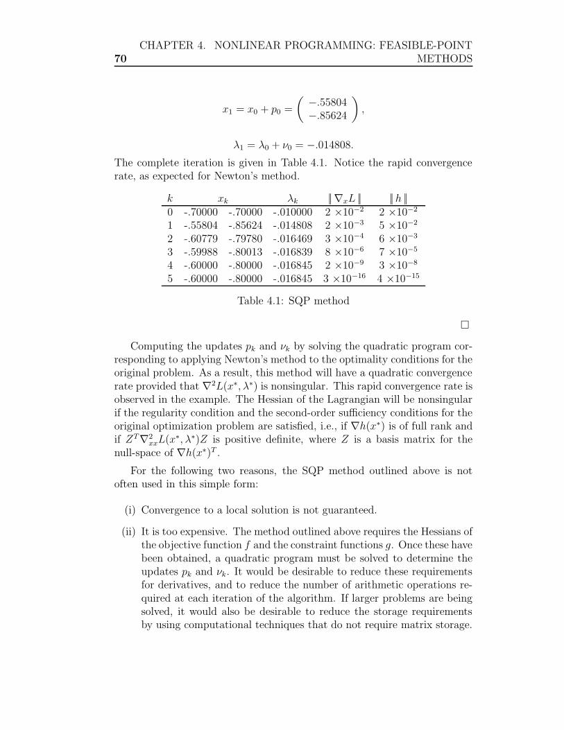
70CHAPTER 4. NONLINEAR PROGRAMMING: FEASIBLE-POINT
METHODS
x1 = x0 + p0 =
(−.55804−.85624
),
λ1 = λ0 + ν0 = −.014808.
The complete iteration is given in Table 4.1. Notice the rapid convergencerate, as expected for Newton’s method.
k xk λk ||∇xL || ||h ||0 -.70000 -.70000 -.010000 2 ×10⁻² 2 ×10⁻²
1 -.55804 -.85624 -.014808 2 ×10⁻³ 5 ×10⁻²
2 -.60779 -.79780 -.016469 3 ×10⁻⁴ 6 ×10⁻³
3 -.59988 -.80013 -.016839 8 ×10⁻⁶ 7 ×10⁻⁵
4 -.60000 -.80000 -.016845 2 ×10⁻⁹ 3 ×10⁻⁸
5 -.60000 -.80000 -.016845 3 ×10⁻¹⁶ 4 ×10⁻¹⁵
Table 4.1: SQP method
Computing the updates pk and νk by solving the quadratic program cor-responding to applying Newton’s method to the optimality conditions for theoriginal problem. As a result, this method will have a quadratic convergencerate provided that ∇2L(x∗, λ∗) is nonsingular. This rapid convergence rate isobserved in the example. The Hessian of the Lagrangian will be nonsingularif the regularity condition and the second-order sufficiency conditions for theoriginal optimization problem are satisfied, i.e., if ∇h(x∗) is of full rank andif ZT∇2
xxL(x∗, λ∗)Z is positive definite, where Z is a basis matrix for thenull-space of ∇h(x∗)T .
For the following two reasons, the SQP method outlined above is notoften used in this simple form:
(i) Convergence to a local solution is not guaranteed.
(ii) It is too expensive. The method outlined above requires the Hessians ofthe objective function f and the constraint functions g. Once these havebeen obtained, a quadratic program must be solved to determine theupdates pk and νk. It would be desirable to reduce these requirementsfor derivatives, and to reduce the number of arithmetic operations re-quired at each iteration of the algorithm. If larger problems are beingsolved, it would also be desirable to reduce the storage requirementsby using computational techniques that do not require matrix storage.

4.4. SEQUENTIAL QUADRATIC PROGRAMMING 71
One way to reduce this expense is to use a quasi-Newton approximation tothe Hessian of the Lagrangian. If this is done, then, second derivatives neednot be computed. in addition, the quasi-Newton matrix can be maintainedin the form of a factorization, and in this way the arithmetic costs of themethod can also be reduced.
Choosing an update formula for the quasi-Newton approximation can bea more complicated decision than in the unconstrained case.
Let us come back to (ii): Convergence results for the SQP programmingmethod are obtained by insisting that (xk+1, λk+1) be a better estimate ofthe solution than (xk, λk). In the unconstrained case, progress is measured interms of the objective function. In our constrained case, progress is measuredin terms of an auxiliary merit function. Usually, a merit function is in the sumof terms that include the objective function and the amount of infeasibility ofthe constraints. If the new point reduces the objective function and reducesinfeasibility, then the value of the merit function will decrease. In manyinstances, however, improvements in the objective value come at the expenseof feasibility, and vice versa, so the merit function must balance these twoaims. One example of a merit function is the quadratic penalty function
M(x) := f(x) + ρ
=:hT (x)︷ ︸︸ ︷(h(x))T h(x)
(= f(x) + ρ
m∑
i=1
h2i (x)
),
where ρ is some positive number (ρ > 0). The grater the value of ρ, thegrater the penalty for infeasibility. This merit function is a function of xonly; other examples of merit functions may be functions of both x and λ.
Example 4.9. Let us use the merit function
M(x) := f(x) + 10hT (x)h(x)
to measure the progress of the SQP method in the previous example. At thefirst iteration
x0 = (−.7000,−.7000)T ,f(x0) = .007447,h(x0) = −.02,
M(x0) = .011447,
and
72CHAPTER 4. NONLINEAR PROGRAMMING: FEASIBLE-POINT
METHODS
x1 = (−.55804,−.85624)T ,f(x1) = .006102,h(x1) = .044563,
M(x1) = .025961,
so, in terms of this merit function, the point x1 is worse than the point x0.At the next iteration, though,
x2 = (−.60779,−.79780)T ,f(x1) = .006641,h(x1) = .005890,
M(x1) = .006988,
indicating that x2 is better than both x1 and x0 for this merit function.
Ideally, the merit function would be chosen so that (x∗, λ∗) would be alocal minimizer of the merit function if and only if it were a local solution ofthe optimization problem. If this were true then a line search with respectto the merit function could be performed:
(xk+1
λk+1
)=
(xk
λk
)+ α
(pk
νk
),
where α is chosen so that
M(xk+1, λk+1) <M(xk, λk).
For this to be successful, the search direction from the quadratic programwould have to be descent direction for the merit function. Unfortunately, itis rarely possible to guarantee that the local minimizers of the merit functionand the local solutions of the optimization problem coincide. For the meritfunction M(x) := f(x) + ρ hT (x)h(x) (quadratic penalty) some of the localminimizers of M approach local solutions of the constrained problem in thelimit as ρ → ∞. In addition, M may have local minima at points whereh(x) 6= 0, i.e., at infeasible points. Other merit functions have analogousdeficiencies that can limit the applicability of convergence theorems, or cancomplicate the development of SQP methods.
In the unconstrained case we assume that search directions are descentdirections with respect to the objective function. Here, we assume thateither pk or the combined vector (pk, νk) is a descent direction with respectto the merit function. A common way to guarantee this is to insist that thereduced Hessian for the quadratic program be positive definite. Come back

4.4. SEQUENTIAL QUADRATIC PROGRAMMING 73
to the constraints. If a quasi-Newton approximation to the Hessian is usedto define the quadratic program, then, positive definiteness of the reducedHessian is often guaranteed by the choice of quasi-Newton update formula.If Newton’s method is used so that the Hessian in the quadratic program is∇2
xxL(xk, λk), then, it is necessary to test if the reduced Hessian is positivedefinite, and to modify if it is not. This testing is more complicated than inthe unconstrained case, particularly if the quadratic program is solved viathe linear system (⊕). In this case, the reduced Hessian may not available.and more elaborate tests for positive definiteness must be used.
Near the solution of the constrained problem, we would normally like totake a step of α = 1 in the line search, so that the quadratic convergence rateof Newton’s method could be achieved. Hence, the merit function should bechosen so that a step of α = 1 is guaranteed to be accepted in the limit as thesolution is approached. For certain merit functions this is not true. In suchcases it is possible to give examples where a step of α = 1 is unacceptable atevery iteration, no matter how close the current point is to the solution.
We will ignore many of these difficulties and only state that pk is a descentdirection for the quadratic penalty merit function. Even more, we will makethe simplifying assumption that the full Hessian of the Lagrangian (or someapproximation to it) is positive definite. If a quasi-Newton approximationto the Hessian is used, this assumption is not reasonable, but for Newton’smethod it is restrictive. The lemma stated subsequently can be used to showthat
limk→∞
∇M(xk) = 0.
For large values of ρ, local solutions of the constrained problem are ap-proximative local minimizers of M(xk) to within O(1/ρ), so this argumentprovides a rough outline of a convergence theorem.
Lemma 4.1. Assume that (pk, νk) is computed as the solution to the quadraticproblem
(QP)kapprox
minimize 1
2pT Hp+ pT
(∇xL(xk, λk)
)
subject to(∇Th(xk)
)p+ h(xk) = 0,
where H is some positive-definite approximation to ∇2xxL(xk, λk). If pk 6= 0,
then
pTk ∇M(xk) < 0

74CHAPTER 4. NONLINEAR PROGRAMMING: FEASIBLE-POINT
METHODS
for all sufficiently large values of ρ, where
M(x) := f(x) + ρhT (x)h(x);
i.e., pk is a descent direction with respect to this merit function.
Proof. See Nash, Sofer (1996).
Finally, let us consider the following problem with inequality constraintsadditionally:
(NLP)
minimize f(x)subject to h(x) = 0,
g(x) ≥ 0.
Here, we can develop an SQP method for this problem as well. Our earlierquadratic program (QP)k was based on a quadratic approximation to theLagrangian function and a linear approximation to the constraints. If thesame approximation is used here, we obtain:
(QP)k
minimize 12pT (∇2
xxL(xk, λk)) p+ pT∇xL(xk, λk)subject to ∇Th(xk)p+ h(xk) = 0,
∇Tg(xk)p+ g(xk) ≥ 0.
The solution (pk, νk)to this quadratic program provide the step to the nextestimate of the solution of the original constrained problem. This problemcan be solved using the active-set method discussed in Section 4.3.
4.5 Reduced-Gradient Methods
Reduced-gradient methods try to maintain feasibility at every iteration. Thisapproach has several advantages:
(i) If each estimate of the solution is feasible, the algorithm can be stoppedbefore it converges and the approximate solution may still be useful.
(ii) Guaranteeing convergence is simpler because progress can be measureddirectly using the value of the objective function, rather than with anauxiliary merit function.

4.5. REDUCED-GRADIENT METHODS 75
The disadvantage of reduced-gradient methods is the computational ex-pense of ensuring that nonlinear constraints remain satisfied at every itera-tion.
We apply a version of the reduced-gradient method to our problem
(NLP)=
minimize f(x)subject to h(x) = 0.
Our derivation begins in the same way as for SQP. The Lagrangian is
L(x, λ) := f(x) − λTh(x),
and, if Newton’s method is applied to the first-order optimality condition,
(xk+1
λk+1
)=
(xk
λk
)+
(pk
νk
),
where pk and νk are obtained as the solution to the linear system
∇2L(xk, λk)
(pk
νk
)= −∇L(xk, λk).
This linear system has the form (cf. Section 4.4):
(⊕)
(∇2
xxL(xk, λk) −∇h(xk)−∇Th(xk) 0
)(pk
νk
)=
(−∇xL(xk, λk)
h(xk)
).
At this point, the derivations for the two methods diverge. In the reduced-gradient method, we use these formulas to derive a portion of the searchdirection, the portion that lies in the null-space of the constraint gradients.If Zk is a basis matrix for the null-space of ∇Th(xk), and Yk is a basis matrixfor the range-space of ∇h(xk), then
pk = ZkpZ + YkpY ,
where pZ is the solution to the reduced problem
ZTk
(∇2
xxL(xk, λk))ZkpZ = −ZT
k ∇xL(xk, λk).
This formula determines pZ in the reduced-gradient method. If all constraintsare linear, then the formula is equivalent to the formula for the reduced

76CHAPTER 4. NONLINEAR PROGRAMMING: FEASIBLE-POINT
METHODS
Newton method derived in Section 4.1. In that case, the matrix Zk will bethe same at every iteration, and
∇2xxL(xk, λk) = ∇2f(xk),
ZTk ∇xL(xk, λk) = ZT
k ∇f(xk).
Hence, the reduced-gradient method is a generalization of the reduced New-ton method for linearly constrained problems. Come back to the generalnonlinear case.
The remaining portion of the search direction is determined from thecondition that the new estimate of the solution must be feasible: h(xk+1) = 0.Since xk+1 = xk + pk, this condition has the form
h(xk + ZkpZ + YkpY ) = 0.
This is a system of m nonlinear equations in the m variables pY . (We assumethat ∇h(xk) is a matrix of null rank.) If the constraints are linear, thenpY = 0. If they are nonlinear, some auxiliary algorithm must be applied tothis nonlinear system to determine pY . For example, Newton’s method couldbe used.
Example 4.10. Let again be given (cf. Example 4.8):
(NLP)=
minimize f(x) := e3x1+4x2
subject to h(x) := x21 + x2
2 − 1 = 0.
The solution being x∗ = (−35,−4
5)T with λ∗ = −5
2e−5 ≈ −.016845. Again, let
x0 = (−.7,−.7)T , even though this point is infeasible. There, ∇f,∇2f, h,∇hand ∇2h were computed in Example 4.8. An estimate of the Lagrange mul-tiplier is needed to determine the gradients and Hessians of the Lagrangian.We compute a multiplier estimate λk by solving
minimizeλ
||∇f(xk) − λ∇h(xk) ||22 .
At x0 the multiplier estimate is λ0 = −.018616. Using this value, we obtain
∇xL = ∇f − λ∇h =
(.008340.015786
),

4.5. REDUCED-GRADIENT METHODS 77
∇2xxL = ∇2f − λ∇2h =
(.08702 .08936.08936 .13915
).
We use variable-reduction to compute the null-space matrix Zk and the range-space matrix Yk based on
∇Th = (2x1, 2x2) = (B,N).
Then,
Zk =
(−B−1N
I
)=
( −x2
x1
1
),
Yk =1√
x21 + x2
2
(x1
x2
).
At this iteration
Z0 =
(−11
).
The null-space portion of the search direction is obtained by solving
ZTk
(∇2
xxL)Zkpk = −ZT
k ∇xL,
or
(.081912)pk = −.0074466,
so that pZ = −.090909.
The remaining portion of the search direction, YkpY , is determined bysolving
h(xk + ZkpZ + YkpY ) = 0.
using Newton’s method. In this example,
YkpY =
(y1
y2
)γ
for some unknown γ, where y1 and y2 are the components of Yk. If we definexk := xk + ZkpZ , then the condition for YkpY has the form

78CHAPTER 4. NONLINEAR PROGRAMMING: FEASIBLE-POINT
METHODS
ϕ(γ) := (x1 + γy1)2 + (x2 + γy2)
2 − 1 = 0.
Applying Newton’s method to this equation gives the iteration
γi+1 = γi −ϕ(γi)
ϕ′(γi)
= γi −(x1 + γiy1)
2 + (x2 + γiy2)2 − 1
2y1(x1 + γiy1) + 2y2(x2 + γiy2).
In this example, we initialize the iteration with γ0 = 0. Then,
γ0 = 0, ϕ(γ0) = −3 × 10⁻³,γ1 = .001753157308727014, ϕ(γ1) = 3 × 10⁻⁶,γ2 = .001751607670563711, ϕ(γ2) = 2 × 10⁻¹²,γ3 = .001751607669352957, ϕ(γ0) = −2 × 10⁻¹⁶.
The overall search direction is
p0 = Z0pZ + Y0pY
=
(−11
)(−.090909) +
(−.70711−.70711
)(.001752)
=
(.089671−.092148
)
and
x1 = x0 + p0 =
(−.61033−.79215
).
The complete iteration is given in Table 4.2. The initial guess of the solutionis not feasible, but all later estimate of the solution are feasible (to 16 digits).The method converges rapidly, as expected for Newton’s method.
k xk λk ||∇xL || ||h ||0 -.70000 -.70000 -.018616 5 ×10⁻³ 2 ×10⁻²
1 -.61033 -.79215 -.016851 4 ×10⁻⁴ 02 -.60001 -.79999 -.016845 3 ×10⁻⁷ 03 -.60000 -.80000 -.016845 1 ×10⁻¹⁶ 1 ×10⁻¹⁶
Table 4.2: Reduced-gradient method.
The reduced-gradient method corresponds to using Newton’s method inthe null-space of the constraints, so it can be expected to converge quadrat-ically in nondegenerate cases. (This quadratic convergence rate is observed

4.5. REDUCED-GRADIENT METHODS 79
in the example above.) As before, Newton’s method is not guaranteed toconverge, and even if it does converge, it may converge to a maximum orstationary point and not a minimum. Hence, some globalization strategymust be employed to ensure convergence to a local solution of (NLP)=.
A line search can be used to guarantee convergence, as was done with theSQP method. If all the solution estimates xk are feasible points, then thevalue of the quadratic penalty merit function is
M(xk) = f(xk) + ρhT (xk)h(xk) = f(xk),
so a line search can be performed using the objective function f itself as amerit function.
The line search for a reduced-gradient method is more complicated thanin the unconstrained case. for each trial value of α, the trial point mustsatisfy
h(xk + αZkpZ + YkpY ) = 0.
Hence, pY depends on α, and must be computed by solving a nonlinearsystem of equations. For large value of α there may not be pY that satisfiesthe constraints, further complicating the line search algorithm. For thesereasons, it is not entirely correct to say that the reduced-gradient methodproduces a search direction, since in fact the method must search along anarc defined by pZ and α.
Concerning descent, we state:
Lemma 4.2. Assume that the reduced-gradient method is applied to the prob-lem (NLP)=. Let xk be the kth estimate of the solution, with h(xk) = 0. Let∇h(x) be of full rank for all x in a neigbourhood of Nk of xk. Also assumethat the null-space portion pZ of the search direction is computed from
ZTk
(∇2
xxL(xk, λk))Zkpk = −ZT
k ∇xL(xk, λk),
where λk is an estimate of the Lagrange multipliers, and where
ZTk
(∇2
xxL(xk, λk))Zk
is positive definite. Define pY (ε) as the solution to
h(xk + εZkpZ + YkpY (ε)) = 0.

80CHAPTER 4. NONLINEAR PROGRAMMING: FEASIBLE-POINT
METHODS
If ZTk ∇xL(xk, λk) 6= 0, then
f(xk + εZkpZ + YkpY (ε)) < f(xk),
for all sufficiently small positive values of ε.
Proof. See Nash, Sofer (1996).
Variants of the reduced-gradient method have been developed that aremore flexible in that they allow some violation of the constraints. such meth-ods might be considered a compromise between reduced-gradient and SQPmethods with their different advantages and disadvantages.

Chapter 5
Nonlinear Programming:Penalty and Barrier Methods
For the feasible-point methods, considered in the previous chapter, there aresome major disadvantages:
(i) As the number of constraints increases, the number of potential sub-problems increases exponentially. While the hope is that the algorithmwill consider only a small proportion of these subproblems, there is noknown method to guarantee that this indeed will be the case.
(ii) The idea of keeping the constraints satisfied exactly, although easilyachieved in the case of linear constraints, is much more difficult toaccomplish in the case of nonlinear constraints, and in some cases maynot be desirable.
In this chapter, we discuss a group of methods, referred to as penalizingmethods, that remove some of these difficulties. Namely, these methods solvea constrained optimization problem by solving a sequence of unconstrainedoptimization problems. The hope is that in the limit, the latter solutionswill converge to the solution of the constrained problem. The unconstrainedproblems involve an auxiliary function that incorporates the objective func-tion or the Lagrangian function, together with penalty terms that measureviolations of the constraints. The auxiliary function also includes one or moreparameters that determine the relative importance of the constraints in theauxiliary function. By changing these parameters appropriately, a sequenceof problems is generated where the effect of the constraints becomes increas-ingly pronounced. In contrast to active-set methods, the auxiliary function

82CHAPTER 5. NONLINEAR PROGRAMMING: PENALTY AND
BARRIER METHODS
takes into account all constraints, even when inequalities are present; thus thecombinatorial difficulties of guessing a correct active set are avoided. Further,since they do not attempt to keep the constraints satisfied exactly, penaliza-tion techniques can be more suitable for handling nonlinear constraints.
5.1 Classical Penalty and Barrier Methods
Here, we have two groups of methods:
(α) one group imposes a penalty for violating a constraint,
(β) the other group imposes a penalty for reaching the boundary of aninequality constraint.
We call (α) penalty methods, and (β) barrier methods.
We start with a geometrical motivation. Let us consider
(P)con
minimize f(x)subject to x ∈M,
where M is the set of feasible points. Define
σ(x) :=
0, if x ∈M,+∞, if x 6∈M,
being such to say, an infinite penalty for violating feasibility. Hence, theproblem (P)con with its constraint can be transformed into an equivalentunconstrained problem
(P)uncon minimize f(x) + σ(x).
Conceptually, if we could solve (P)uncon, we would be done: a point x∗ solves(P)con if and only if it solves (P)uncon. Unfortunately, this is not a practicalidea, since the objective function of the unconstrained minimization is notdefined outside of the feasible region. Even if we were to replace the “∞”by a large number, the resulting unconstrained problem would be difficult tosolve because of its discontinuities.

5.1. CLASSICAL PENALTY AND BARRIER METHODS 83
Instead, barrier and penalty methods solve a sequence of unconstrainedsubproblems that are more manageable, and that gradually approximate theproblem (P)uncon. This is achieved by replacing the ideal penalty σ by acontinuous function which gradually approaches σ.
In barrier methods, this function (called barrier term) approaches σ fromthe interior of the feasible region. It creates a barrier that prevents the iter-ates from reaching the boundary of the feasible region. in penalty methods,this function (called a penalty term) approach σ from the exterior of thefeasible region. It serves as a penalty for being infeasible.
Barrier methods generate a sequence of strictly feasible iterates which con-verge to a solution of the problem from the interior of the feasible region. Forthis reason, they are called interior-point methods; in Chapter 3 we studiedthem in the special case of linear programming! Since these methods requirethe interior of the feasible region to be 6= ∅, they are not more appropriatefor problems without equality constraints (see, however, our discussion in thelinear case, including infeasibility, in Chapter 3).
In contrast, penalty methods permit the iterates to be infeasible. A gradu-ally increasing penalty is imposed for violation of feasibility, however. Penaltymethods usually generate a sequence of points that that converge to a solu-tion of the problem from the exterior of the feasible region. These methodsare usually more convenient on problems with equality constraints.
Despite their apparent differences, barrier and penalty methods havemuch in common. Their convergence theories are similar, and the underly-ing structure of their unconstrained problems is similar. Much of the theoryfor barrier methods can be replicated for penalty methods and vice versa.It is common to use the generic name “penalty methods” to describe bothmethods, with interior penalty methods referring to (β) (barrier methods),and exterior penalty methods referring to (α) (penalty methods).
Barrier Methods:Consider the problem
(NLP)≥
minimize f(x)subject to g(x) ≥ 0,
where g := (g1, g2, . . . , gs)T ; f and g being of class C2. Barrier methods are
strictly feasible methods, i.e., the iterates lie in the interior of the feasible re-gion. We assume, therefore, that the feasible set M has a nonempty interior:
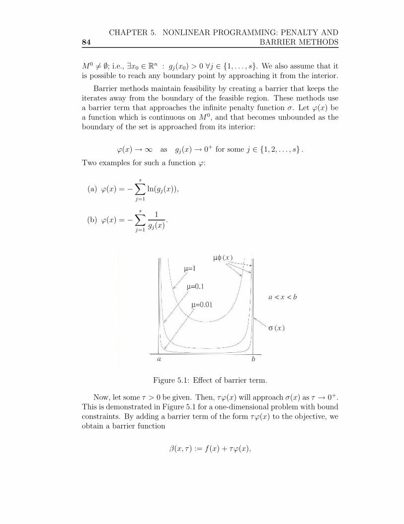
84CHAPTER 5. NONLINEAR PROGRAMMING: PENALTY AND
BARRIER METHODS
M0 6= ∅; i.e., ∃x0 ∈ Rn : gj(x0) > 0 ∀j ∈ 1, . . . , s. We also assume that it
is possible to reach any boundary point by approaching it from the interior.
Barrier methods maintain feasibility by creating a barrier that keeps theiterates away from the boundary of the feasible region. These methods usea barrier term that approaches the infinite penalty function σ. Let ϕ(x) bea function which is continuous on M 0, and that becomes unbounded as theboundary of the set is approached from its interior:
ϕ(x) → ∞ as gj(x) → 0+ for some j ∈ 1, 2, . . . , s .Two examples for such a function ϕ:
(a) ϕ(x) = −s∑
j=1
ln(gj(x)),
(b) ϕ(x) = −s∑
j=1
1
gj(x).
Figure 5.1: Effect of barrier term.
Now, let some τ > 0 be given. Then, τϕ(x) will approach σ(x) as τ → 0+.This is demonstrated in Figure 5.1 for a one-dimensional problem with boundconstraints. By adding a barrier term of the form τϕ(x) to the objective, weobtain a barrier function
β(x, τ) := f(x) + τϕ(x),

5.1. CLASSICAL PENALTY AND BARRIER METHODS 85
where τ is referred to as the barrier parameter. The best known barrierfunction is the logarithmic barrier function
β(x, τ) := f(x) + τ
s∑
j=1
ln(gj(x)),
but the inverse barrier function
β(x, τ) := f(x) + τ
s∑
j=1
1
gj(x),
is also widely used. Barrier methods solve a sequence of unconstrained prob-lems:
(NLP)kuncon minimize
xβ(x, τk)
for a sequence(τk)
k∈N0of barrier parameters τk > 0 that decrease monoton-
ically to zero: τk+1 ≤ τk ∀k ∈ N0, τk → 0+ (k → ∞).
As the barrier term is ∞ at the boundary ∂M of the feasible set M , itacts as a repelling force which derives the minimizers of the barrier functionaway from the boundary into the interior M 0 of the feasible region. Thus,any minimizer of the barrier function will be strictly feasible. As the barrierparameter is decreased, however, the effect of the barrier term is diminished,so that the iterates can gradually approach the boundary ∂M .
Why do we solve a sequence of problems? It might seem better to solve asingle unconstrained problem using a small µ –but this is usually not practi-cal: When τ is small, the problems are difficult to solve (τϕ is close in shapeto the infinite penalty σ). If τ is decreased gradually, and if the solution ofone unconstrained problem is used as the starting point of the next problem,these unconstrained problems tend to be much easier to solve.
Example 5.1. Consider the nonlinear program
(NLP)≥
minimize f(x) := x1 − 2x2
subject to 1 + x1 − x22 ≥ 0,x2
2 ≥ 0.
Then, the logarithmic barrier function gives the unconstrained problems

86CHAPTER 5. NONLINEAR PROGRAMMING: PENALTY AND
BARRIER METHODS
(NLP)kuncon minimize
xβ(x, τk) := x1 − 2x2 − τk ln(1 + x1 − x2
2) − τk ln x2
for a sequence of decreasing µk. For a specific µk, the first-order necessaryoptimality conditions are:
(NOC)k
1 − τk1 + x1 − x2
2
= 0,
−2 − 2τkx2
1 + x1 − x22
− τkx2
= 0.
If the constraints are strictly satisfied, then, the denominators are positive.We obtain an equation for x2:
x22 − x2 −
1
2τ = 0,
giving
x2(τ) :=1 +
√1 + 2τ
2(τ := τk)
(why is the positive root taken?). Since x1 = x22 − 1 + τ , we get
x1(τ) :=
√1 + 2τ + 3τ
2.
The unconstrained objective is strictly convex, hence, this solution is theunique local minimizer in the feasible region. As µ approaches 0 (i.e., whenk → ∞), we obtain
limτ→0+
(x1(τ)x2(τ)
)=
√1+2(0)+3(0)−1
21+√
1+2(0)
2
=
(01
)=: x∗.
It is easy to verify that this point x∗ is indeed the solution of (NLP)≥.
Table 5.1 shows the values of x1(τ) and x2(τ) for a sequence of barrierparameters τ = τk. The initial parameter is related to be τ0 := 1, andconsecutive parameters are decreased by a factor of 10. Observe that x(τ) =(x1(τ), x2(τ))
T exhibits a linear rate of convergence to the optimal solution.

5.1. CLASSICAL PENALTY AND BARRIER METHODS 87
τ x1(τ) x2(τ)100 1.8660254 1.366025410−1 0.1977226 1.047722610−2 0.0199752 1.004975210−3 0.0019998 1.000499810−4 0.0002000 1.000050010−5 0.0000200 1.000005010−6 0.0000020 1.0000005
Table 5.1: Barrier function minimizers.
The previous examples illustrates a number of features that typicallyoccur in a barrier method:
(i)(x(τk)
)k∈N0
converges to a optimal solution x∗. (It is possible to prove
convergence for barrier methods under mild conditions.)
(ii) τ 7→ x(τ) (τ > 0) is a differentiable function, called the barrier tra-jectory. If the logarithmic or inverse barrier method are used, it ex-ists, provided x∗ is a regular point of the constraints that satisfies thesecond-order sufficiency conditions. As well as the strict complemen-tarity conditions. The existence of a trajectory can be used to developalgorithms such as path-following algorithms for LP (similar to Chap-ter 3). It can also be used to develop techniques that accelerate theconvergence of a barrier method.
(iii) Under a regularity condition again, for both the logarithmic and theinverse barrier functions, we find estimates µ(τ) of the Lagrange mul-tiplier µ∗ at the optimal point x∗. We explain this subsequently.
To (iii): We discuss it for the case of the logarithmic barrier function. Con-sider a point x = x(τ) which is a minimizer of the logarithmic barrier functionfor a specific parameter τ . Setting the gradient of the barrier function (withrespect to x) to zero, we obtain
∇f(x) − τ
s∑
j=1
1
gj(x)∇gj(x) = 0
if and only if
∇f(x) −s∑
j=1
τ
gj(x)︸ ︷︷ ︸=:µj(τ)
∇gj(x) = 0

88CHAPTER 5. NONLINEAR PROGRAMMING: PENALTY AND
BARRIER METHODS
(at x = x(τ)). We therefore have a feasible point x(τ) and a vector µ(τ)satisfying the first-order necessary optimality conditions, except τ (insteadof 0) on the right-hand side of (cf. (NOC)τ
sf in Section 3.2.):
(NOC)τsf
∇f(x(τ)) −∑sj=1 µj(τ)∇gj(x(τ)) = 0
µj(τ)gj(x(τ)) = τ
µj(τ)≥
(>)0
∀j ∈ 1, 2, . . . , s
and (strict) feasibility.
As τ → 0+, µ(τ) can be viewed as an estimate of µ∗, the Lagrangemultiplier at x∗. (Indeed, if x∗ is a regular point, then: x(τ) → x∗ (τ →0) =⇒ µ(τ) → µ∗ (τ → 0).)
Example 5.2. Consider the nonlinear problem
(NLP)≥
minimize f(x) := x21 + x2
2
subject to x1 − 1 ≥ 0,x2 + 1 ≥ 0,
the solution being x∗ = (1, 0)T . The inequality j = 1 is active at x∗, and thecorresponding Lagrange multiplier is µ∗
1 = 2. Suppose the problem is solvedvia a logarithmic barrier method. Then, this method solves
(NLP)kuncon minimize
xβ(x, τ) = x2
1 + x22 − τ ln(x1 − 1) − τ ln(x2 + 1)
for a decreasing sequence of barrier parameters τ = τk which converge to 0.Now, (NOC)τ
sf gives
2x1 −τ
x1 − 1= 0,
2x2 −τ
x2 + 1= 0,
yielding
x1(τ) =1 +
√1 + 2τ
2, x2(τ) =
−1 −√
1 + 2τ
2.

5.1. CLASSICAL PENALTY AND BARRIER METHODS 89
The corresponding Lagrange multiplier estimates are:
µ1(τ) =τ
x1(τ) − 1=
√1 + 2τ + 1,
µ2(τ) =τ
x2(τ) + 1=
√1 + 2τ − 1,
When τ → 0, we obtain
limτ→0
(x1(τ)x2(τ)
)
︸ ︷︷ ︸=x(τ)
=
(10
)
︸ ︷︷ ︸=:x∗
and limτ→0
(µ1(τ)µ2(τ)
)
︸ ︷︷ ︸=µ(τ)
=
(20
)
︸ ︷︷ ︸=:µ∗
.
Despite their attractive features, barrier methods also have potential dif-ficulties; we mention the most important one: The unconstrained problemsbecome increasingly difficult to solve as the barrier parameter decreases. Thereason is that (with the exception of some special cases) the condition numberof the Hessian matrix of the barrier function at its minimum point becomesincreasingly large, tending to ∞ as τ → 0.
Example 5.3. We come back to our Example 5.2. There,
∇2xxβ(x, τ) =
2 +τ
(x1 − 1)20
0 2 +τ
(x2 + 1)2
.
Suppose now, that x(τ) is a minimizer of β(·, τ) for some τ > 0. Recall fromExample 5.2 that
µ1(τ) =τ
x1(τ) − 1and µ2(τ) =
τ
x2(τ) + 1.
When τ ≈ 0, then, µ1(τ) ≈ 0. Therefore,
∇2xxβ(x(τ), τ) =
2 +µ2
1(τ)
τ0
0 2 +µ2
2(τ)
τ
≈
(2 +
4
τ0
0 2
).
The condition number of this matrix (i.e., the product of both its matrixnorm and the one of its inverse; exercise) is approximately equal to

90CHAPTER 5. NONLINEAR PROGRAMMING: PENALTY AND
BARRIER METHODS
2 + 4τ
2= 1 +
2
τ= O(
1
τ),
hence, the matrix is ill conditioned (highly sensitive against smallest per-turbations). Although the calculations were performed for a point on thebarrier trajectory, the same will hold at all points in a neighbourhood of thesolution.
The contours of the barrier function in this example are shown in Fig-ure 5.2 for τ = 1 and τ = 0.1. We see that for the smaller τ , the contours(level sets, i.e., the “finger print” of β(·, τ)) are almost parallel to the linex1 = 1. More precisely, the contours are almost parallel to the null-space ofthe gradient of the active constraint at the solution. This is characteristic ofbarrier functions.
Figure 5.2: Contours of the logarithmic barrier function.
The ill conditioning of the Hessian matrix of β(·, τ) has several ramnifi-cations. It rules out the use of an unconstrained method whose convergencerate depends on the condition number of the Hessian matrix at the solution.Therefore, Newton-type methods are usually the method of choice. The so-lution to the Newton equations is also sensitive to the ill condition of theHessian matrix, however. The numerical errors can result in a poor searchdirection.
In the early 1970s, the ill conditioning of the barrier functions led totheir abandonment. Interest in barrier methods was renewed in 1984, withthe announcement of Karmarkar’s method for LP and the discovery shortlythereafter that this method is just a special case of a barrier method (cf. ourdiscussions above, and Chapter 3)!

5.1. CLASSICAL PENALTY AND BARRIER METHODS 91
Recently, special attention has been given to the development of special-ized linear algebra techniques that compute a numerically stable, approxi-mate solution to the Newton equations for a barrier function. We discussedthem in Section 3.2 (path-following methods).
Penalty Methods:In contrast to barrier methods, penalty methods solve a sequence of un-constrained optimization problem whose solution is usually infeasible to theoriginal constrained problem. A penalty for violation of the constraints isincurred, however. As this penalty is increased, the iterates are forced to-wards the feasible region. An advantage of penalty methods is that they donot require the iterates to be strictly feasible. Thus, unlike barrier methods,they are suitable for problems with equality constraints.
Consider first the equality-constrained problem
(NLP)=
minimize f(x)subject to h(x) = 0,
where f and h := (h1, h2, . . . , hm)T are assumed to be of class C2. Thepenalty for constraint violation will be a continuous function ψ with thefollowing property:
< ∗ > ψ(x) = 0, if x ∈ M (feasibility),ψ(x) > 0, otherwise.
The best-known such penalty is the quadratic-loss function
(a) ψ(x) =1
2
m∑
i=1
h2i (x) =
1
2hT (x)h(x).
Also possible is a penalty of the form
(b) ψ(x) =1
γ
m∑
i=1
|hγi (x) | , where γ ≥ 1.
The wight of the penalty is controlled by a penalty parameter ρ. As ρ in-creases, ρψ approaches the “ideal penalty” σ: ρψ(x) → σ(x) (ρ → ∞). Byadding ρψ to f we obtain the penalty function
92CHAPTER 5. NONLINEAR PROGRAMMING: PENALTY AND
BARRIER METHODS
π(x, ρ) := f(x) + ρψ(x).
The penalty method consists in solving a sequence of unconstrained problemsof the form
(NLP)kuncon minimize
xπ(x, ρk)
for an increasing sequence(ρk
)k∈N0
of ρk > 0 tending to infinity:
ρk ≤ ρk+1 ∀k ∈ N0,
ρk → ∞ (k → ∞).
In general, the minimizers of the penalty function violate the constraintsh(x) = 0. The growing penalty gradually forces these minimizers towardsthe feasible region.
Penalty methods share many of the advantages of the barrier methods:
(i) Under mild conditions, it is possible to guarantee convergence.
(ii) Under mild conditions, the sequence of penalty function minimizersdefines a continuous trajectory.
(iii) In the latter case, it is possible to get estimates of the Lagrange mul-tipliers at the solution.
For example, consider the quadratic-loss penalty function
π(x, ρ) = f(x) +1
2ρ
m∑
i=1
h2i (x).
Its minimizer x(ρ) satisfies
∇xπ(x(ρ), ρ) = ∇f(x(ρ)) + ρm∑
i=1
∇hi(x(ρ))hi(x(ρ))
= 0,
that is,

5.1. CLASSICAL PENALTY AND BARRIER METHODS 93
∇f(x(ρ)) −m∑
i=1
(− ρhi(x(ρ))
)
︸ ︷︷ ︸=:λi(ρ)
∇hi(x(ρ)) = 0.
If x(ρ) converges to x∗ being a solution and regular with respect to theconstraints, then, λ(ρ) converges to the Lagrange multiplier λ∗ associatedwith x∗:
x(ρ) → x∗ (ρ→ ∞) =⇒ λ(ρ) → λ∗ (ρ→ ∞).
Penalty functions suffer from the same problems of the ill conditioningas do barrier functions! As ρ increases, the condition number of the Hes-sian matrix of π(x(ρ), ρ) increases, tending to ∞ as ρ → ∞. Therefore theunconstrained minimization can become increasingly difficult to solve.
It is possible to apply penalty methods to problems with inequality con-straints. Consider in class C2, e.g.,
(NLP)≥
minimize f(x)subject to g(x) ≥ 0,
where g := (g1, g2, . . . , gs)T . Any continuous function which satisfies < ∗ >
can serve as a penalty. Thus, for example, the quadratic-loss penalty in thiscase is
ψ(x) =1
2
s∑
j=1
(min gj(x), 0
)2.
This function has continuous first derivatives
∇ψ(x) =
s∑
j=1
(min gj(x), 0
)∇gj(x),
but its second derivatives can be discontinuous at points where some con-straint gj is satisfied exactly. The same observation holds for other simpleforms of the penalty function. Thus, we cannot safely use Newton’s methodto minimize the function. For this reason, straightforward penalty methodshave not been widely used for solving general inequality-constrained prob-lems.

94CHAPTER 5. NONLINEAR PROGRAMMING: PENALTY AND
BARRIER METHODS
Convergence of Penalization Methods:Let us focus on the convergence of barrier methods when applied to theinequality-constrained problem
(NLP)≥
minimize f(x)subject to g(x) ≥ 0.
We denote the feasible set by M again, and write
Msf :=x ∈ R
n∣∣ gj(x) > 0 (j ∈ 1, 2, . . . , s)
;
generically, under some regularity condition: Msf = M0.
In preparing our convergence theorem, we make the following assump-tions:
(A1) f and g are continuous.
(A2) ∀α ∈ R :x ∈ R
n∣∣ x ∈M, f(x) ≤ α
(A3) Msf 6= ∅.
(A4) M = Msf (topological closure).
Assumptions (A1-2) imply that f has a minimum value on the set M (why?).Assumption (A3) is necessary to define the barrier subproblems. Assumption(A4) is necessary to avoid situations where the minimum point is isolated,and does not have neighbouring interior points.
For example, consider f(x) := x to be minimized subject to the con-straints x2 − 1 ≥ 0 and x+ 1 ≥ 0. Then
M = [1,∞) ∪ −1,where the isolated point x∗ = −1 is the minimizer, but because it is isolatedit is not possible to approach it from the interior of the feasible region, anda barrier method could not converge to this solution.
The barrier function will be of the form
β(x, τ) = f(x) + τϕ(x),
where ϕ can be any function that is continuous on M 0, and that satisfies

5.1. CLASSICAL PENALTY AND BARRIER METHODS 95
ϕ(x) → ∞ as gj(x) → 0+.
We will state that under mild conditions, the sequence of barrier mini-mizers has a convergent subsequence, and the limit of any such convergentsubsequence is a solution to the problem. Although in practice convergenceof the entire sequence of minimizers is observed, from a theoretical point ofview it is not always possible to guarantee convergence of the entire sequence,but only convergence of some subsequence:
Example 5.4. Consider the one-variable problem
(NLP)≥
minimize − x2
subject to 1 − x2 ≥ 0.
The logarithmic barrier function is β(x, τ) = −x2 − τ ln(1 − x2). It has asingle minimizer x∗ = 0 if τ = 1, and two minimizers x∗ = ∓
√1 − τ if τ < 1.
(The point x∗ = 0 is a local minimizer if τ < 1) Suppose that τ0, τ1, τ2, . . . isa sequence of decreasing barrier parameters < 1. Then, a possible sequenceof minimizers of β(·, τk) is
xk = (−1)k√
1 − τk.
This sequence oscillates between neighbourhoods of −1 and +1, and, hence,nonconvergent! However, the subsequences
(x2ν
)ν∈N0
and(x2ν+1
)ν∈N0
both
converge to solutions of (NLP)≥!
Theorem 5.1. Suppose that our given problem (NLP)≥ satisfies Assump-tions (A1-4), and that a sequence of unconstrained minimization problems
(NLP)kuncon minimize
xβ(x, τk) = f(x) + τkϕ(x)
is solved for 0 < τk+1 < τk ∀k ∈ N0, limk→∞
τk = 0. Furthermore, suppose
that the functions β(·, τk) have a minimum in Msf ∀k ∈ N0. Let this globalminimizers be called xk.
Then,
(a) f(xk+1) ≤ f(xk) ∀k ∈ N0 (descent);

96CHAPTER 5. NONLINEAR PROGRAMMING: PENALTY AND
BARRIER METHODS
(b) ϕ(xk+1) ≥ ϕ(xk) ∀k ∈ N0;
(c)(xk
)k∈N0
has a convergent subsequence;
(d) if(xκν
)ν∈N0
is any convergent subsequence of unconstrained minimizers
of β(·, τκν), then, its limit point is a global solution x∗ of (NLP)≥.
Proof. See Nash, Sofer (1996).
A key assumption in this theorem is that the barrier functions have aminimizer. We now state a condition which guarantees this:
Lemma 5.1. Assume that M is compact. Then, for any fixed positive valueτ , there exists a point x(τ) ∈Msf which minimizes β(·, τ).
Proof. See Nash, Sofer (1996), or exercise.
Another case where the barrier minimizers always exist, is when the prob-lem is convex, even when M is unbounded.
Convergence results for penalty methods can be developed in a similarmanner.

Bibliography
[1] G. Golub and C.V. Loan, Matrix Computations. The Johns Hopkins Uni-versity Press, Baltimore, 1989.
[2] N.I.M. Gould and S. Lyffer, An introduction to algorithms for nonlinearoptimization, RAL-TR-2002-031, Computational Science and Engineer-ing Department, Atlas Centre, Rutherford Appleton Laboratory, Oxford-shire, 2003.
[3] H. Hamacher and K. Klamroth, Lineare und Netzwerkoptimierung. Lin-ear and Network Optimization. Ein bilinguales Lehrbuch, Viewegs Ver-lagsgesellschaft, 2000.
[4] H.Th. Jongen, K. Meer and E. Triesch, Optimization Theory, Kluwer,forthcoming.
[5] S. G. Nash and A. Sofer, Linear and Nonlinear Programming, McGraw-Hill, 1996.
[6] J. Nocedal and S. J. Wright. Numerical Optimization, Springer Series inOperations Research. Springer, 1999.
[7] P. Spellucci, Numerische Verfahren der nichtlinearen Optimierung, ISNMLehrbuch, Birkhauser Verlag, 1993.