Perturbation — 1

Lecture Notes: Perturbation and Large Scale Structure

Sep/Oct, 2016

So far, we’ve studied homogeneous cosmology. Our universes have had the same density at all

points in space and have merely evolved in time. This has allowed us to make statements

about the thermal history and fate of the universe. However, if we want to study objects

like galaxies, we have to consider departures from homogeneity.

Galaxies and clusters of galaxies are complex systems, but the aim of cosmologist is not to

explain all their details - that’s the goal of galaxy class, astrophysicist. Here we week

to explain the origin of large scale structure of the universe, and how does it develop in

later universe. We define the density enhancement δρ, and the density contrast ∆ = δρ/ρ.

When δ << 1, these perturbations grow linearly (actually it is linearly with scale factor

in standard models). However, when these amplitude approaches unity, their subsequent

development becomes non-linaer and they rapidly evolve into bound objects, such as galaxies

and clusters of galaxies, when many non-linear astrophysical effects become important, such

as star formation and feedback. Our second part of this course is to deal with mostly small,

linear perturbations and the observations of large scale structure, and how to use them

to probe our cosmological model. Here our objectives are twofold, (1) to understand how

density perturbations evolve in an expanding universe, and (2) to derive and account for the

initial conditions necessary for the formation of the structures we observe.

In the first few lectures of this part of the course, we will mostly due with the first question. We

will go over how density and velocity perturbations grow in the universe, and then introduce

statistics of large scale structure and the means to observe them at low redshift. Then we

will treat the fluctuations of the CMB as a special case, which is especially important in

understanding some of the initial condition issues and its impact in our understanding of the

early universe.

Before diving into the math, some back-of-the-envelop considerations of the scale that we are

talking about. You can simply calculate the mass density of a galaxy (∼ 10 kpc), a cluster

of galaxy (∼ 1 Mpc), and then a supercluster, or large scale structure you see in redshift

surveys (∼ 10 Mpc). Comparing that to the mass density of the universe, e.g, for Ω = 0.3.

Turns out that ∆ = δρ/ρ is 106, 103 and a few, respectively. Note that for a bound object,

such as a galaxy, δρ, its density will not change with the expansion of the universe: it is

a bound object, which means that the local gravitational field has already overcome the

expansion and it is viralized and doesn’t grow or collapse anymore (to the zeroth order, it

doesn’t change subtly). Since ρ ∼ (1+z)3, that means that for galaxies, we will reach ∆ ∼ 1

Perturbation — 2

at z ∼ 100 or so if nothing else happens. This immediately gives you that we should begin

to consider galaxy formation from redshift of a hundred or lower, and clusters at z < 10.

Turns out that most galaxies started to form at lower redshift but not by more than an order

of magnitude. So this gives you the basic scale of the redshift range that we care about.

1 Growth of small perturbations in the expanding universe

The universe is obviously lumpy on small scales, and we have argued that it gets smoother

on large scales. This is the justification for considering the inhomogeneity as a perturbation

to the homogeneous solution.

We have already done this kind of analysis once in the case of the ISM. We found a Jeans

instability, in which perturbations grew exponentially if they had a longer wavelength than

the Jeans wavelength and were stabilized by pressure otherwise.

Now we’ll repeat this analysis in the case of an expanding universe.

We again begin from the basic hydro equations

dcρ

dct+ ρ∇x · v = 0

dcv

dct= −1

ρ∇xp−∇xΦ

∇2xΦ = 4πGρ

where the dc/dct notation indicates a Lagrangian derivative and the ∇x are derivatives

with respect to the physical coordinate x. This is the notation in fluid dynamics with a

coordinate system that motion of a particular fluid element is followed. The first equation

is the continuity equation, the second is the equation of motion, or Euler equation, and the

third describes the gravitational potential, the Poission equation.

You might be more familiar with the other coordinate system in fluid dynamics, the Euler

system, in which we apply partial derivatives to qualities as a function of a fixed grid of

coordnates,dcdct

=∂

∂t+ (v · ∇x).

So in real calculations, such as when you carry out cosmological simulations, there are advan-

tages and disadvantages of using either Euler or Lagrangian systems when setting up your

calculations. We are dealing with cosmology, and with particles that are almost fixed in

Perturbation — 3

Hubble flow, so one more complication is that we want to express things in comoving coordi-

nate. In particular, we define x = Rr where R(t) is the usual expansion factor. This means

∇r = R∇x.

We then split the velocity into a Hubble expansion term and a peculiar velocity term, v =

Hx + δv = Hx + Ru. u is the comoving peculiar velocity, i.e. how far a particle moves in

comoving coordinates per unit time.

δv is called a peculiar velocity. It’s the velocity difference relative to the expectation of the

Hubble law.

We will then switch from a Lagrangian derivative to a derivative in the comoving frame. This

means that

dcdct

=∂

∂t+ (v · ∇x) =

∂

∂t+ (Hx · ∇x) + (δv · ∇x) =

d

dt+ (u · ∇r),

where d/dt is differential over the comoving grids.

Finally, we will find it convenient to measure densities in fractional units relative to the back-

ground density ρh(t). So ρ = (1 + δ)ρh.

We now can insert these substitutions and remove the homogeneous part of the solution.

For the continuity equation, we get

dρ

dt+ (u · ∇r)ρ+ ρ∇x · (Hx +Ru) = 0

ρhdδ

dt+ (1 + δ)

dρhdt

+ ρh(u · ∇r)δ + (1 + δ)ρh(3H +∇r · u) = 0

dρhdt

=d(ρ(0)R−3)

dt= −3ρ0R

−4dR/dr = −3Hρh

Note that ∇x · x = 3. This means that the homogeneous terms cancel, leaving us with

dδ

dt+ (u · ∇r)δ + (1 + δ)∇r · u = 0

This looks very much like a continuity equation, but now it’s on perturbed quantities.

We can play similar games with the Euler and Poisson equation. We get

dv

dt+ (u · ∇r)v = −1

ρ∇xp−∇xΦ

The first term becomes dv/dt = d(Hx)/dt+ (dR/dt)u +R(du/dt), and the first term of this

cancels the homogeneous part of the potential. The second term here generates two terms,

the first of which is (u · ∇r)Hx = RuH. This will have important consequences.

du

dt+ 2Hu + (u · ∇r)u = − c

2s

R2

∇rδ

1 + δ− 1

R2∇rφ

Perturbation — 4

Here we consider the universe is expanding adiabatically, and the perturbation in energy and

density are related to the adiabatic sound speed:

∂p/∂ρ = c2s

, and Poisson equation becomes:

∇2rφ = 4πGR2ρhδ

Here Φ = φ0 + φ

These are the full equations for gravitational perturbations in comoving coordinates. They are

non-linear.

Now let’s consider small perturbations. We keep only linear terms.

dδ

dt= −∇r · u

du

dt+ 2Hu = − c

2s

R2∇rδ −

1

R2∇rφ

∇2rφ = 4πGR2ρhδ

We take the negative divergence of the Euler equation

−d∇r · udt

− 2H∇r · u =c2sR2∇2rδ +

1

R2∇2rφ

d2δ

dt2+ 2H

dδ

dt=

c2sR2∇2rδ + 4πGρhδ

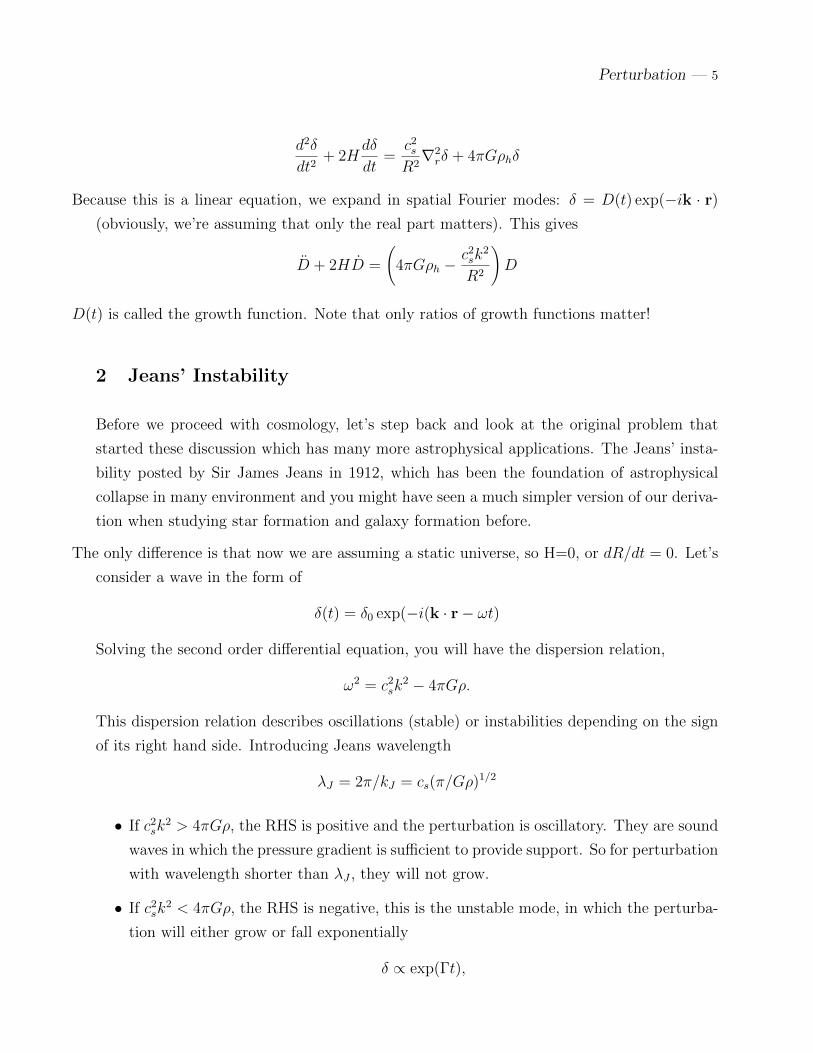
Because this is a linear equation, we expand in spatial Fourier modes: δ = D(t) exp(−ik · r)

(obviously, we’re assuming that only the real part matters). This gives

D + 2HD =

(4πGρh −

c2sk2

R2

)D

D(t) is called the growth function. Note that only ratios of growth functions matter!

So far, we discussed the evolution of perturbations in an expanding universe. We started from

the standard fluid dynamics equations, then we transformed it into co-moving units to care

of the expansion of the universe. We then introduced perturbative terms, density contrast δ

and peculiar velocity u. We derived the full continuity equation, Euler equation and Poission

equation in an expanding universe, expressed in comoving units, in perturbative quantities.

Finally, we assume the perturbation is small and neglect high order terms, and arrived at:

Perturbation — 5

d2δ

dt2+ 2H

dδ

dt=

c2sR2∇2rδ + 4πGρhδ

Because this is a linear equation, we expand in spatial Fourier modes: δ = D(t) exp(−ik · r)

(obviously, we’re assuming that only the real part matters). This gives

D + 2HD =

(4πGρh −

c2sk2

R2

)D

D(t) is called the growth function. Note that only ratios of growth functions matter!

2 Jeans’ Instability

Before we proceed with cosmology, let’s step back and look at the original problem that

started these discussion which has many more astrophysical applications. The Jeans’ insta-

bility posted by Sir James Jeans in 1912, which has been the foundation of astrophysical

collapse in many environment and you might have seen a much simpler version of our deriva-

tion when studying star formation and galaxy formation before.

The only difference is that now we are assuming a static universe, so H=0, or dR/dt = 0. Let’s

consider a wave in the form of

δ(t) = δ0 exp(−i(k · r− ωt)

Solving the second order differential equation, you will have the dispersion relation,

ω2 = c2sk2 − 4πGρ.

This dispersion relation describes oscillations (stable) or instabilities depending on the sign

of its right hand side. Introducing Jeans wavelength

λJ = 2π/kJ = cs(π/Gρ)1/2

• If c2sk2 > 4πGρ, the RHS is positive and the perturbation is oscillatory. They are sound

waves in which the pressure gradient is sufficient to provide support. So for perturbation

with wavelength shorter than λJ , they will not grow.

• If c2sk2 < 4πGρ, the RHS is negative, this is the unstable mode, in which the perturba-

tion will either grow or fall exponentially

δ ∝ exp(Γt),

Perturbation — 6

Where Γ = ±[4πρG(1−λ2J/λ2)]−1/2. The positive sign corresponds to growing mode. For

very long wavelength, the growth rate Γ ∼ (Gρ)1/2, or the growth time τ ∼ (Gρ)−1/2.

This is your dynamical timescale for a spherical collapse.

The physics for Jeans instability is simple. We have hydrostatic pressure support:

dp/dr = −GM(< r)/r2,

The region becomes unstable when gravity overwhelms pressure support. So dp/dr ∼ p/r ∼c2sρ/r and M ∼ ρr3, then we will have for r > rJ ∼ cs/(Gρ)1/2, it becomes Jeans un-

stable. The other way to put it is sound crossing time r/cs is less than dynamical time

1/(G/rho)1/2, then it becomes unstable. We will see Jeans instability again when discussing

galaxy formation.

3 Jeans’ instability in an expanding universe

Before, we had an equation with time-independent coefficients, so we could use time expo-

nentials. This led to a dispersion relation that indicated that k < kJ grew exponentially.

Now, H and ρh both depend on time, so exponentials aren’t the correct solution. Since we are

worrying out large scale structure, we will only consider long wavelength λ >> λJ , in which

case we neglect the pressure term.

D + 2HD = 4πGρhD

Let’s consider a matter-dominated universe (Ω = 1) in which cs = 0. This means that H = 23t

and 8πGρh = 3H2 = 43t2

. Hence, we have

D +4

3tD − 2

3t2D = 0

This has a form that can be solved by power-laws, so let’s try D = tn. This gives

n(n− 1) +4n

3− 2

3= 0

which has solutions 2/3 and −1. This means that we have one mode that grows in time,

and another that decays.

Next, we remember that R = t2/3. So our growing mode has its amplitude growing as R, while

the decaying mode decreases as R−3/2.

We no longer have exponential growth! The expansion of the universe slows the growth to

a power-law! In particular, since the perturbation growth with the exact same dependent

Perturbation — 7

on t as R, this means perturbation growth self-similarly as the expansion of the universe,

δ ∝ (1 + z)−1, so in a critical universe, new structure is always forming because the universe

is self-similar.

We can also work out the case in which the universe is empty, R = constant, and ρ = 0, i.e.,

the Milne model, in this case,

D + 2HD = 0,

and H = 1/t. Seeking power law solution, we find n = 0 or n = −1, so there is a constant

mode and a decay mode. Perturbation won’t grow in an empty universe.

In general, one can write down the solution for the growing mode as

∆(R) = 5/2Ωm0H∫ R

0dR′/(dR′/dt)3

where R is the scale factor. And for a low density universe, it goes through two stages, at

z >> 1, the density parameter Ωm ∼ 1, so the perturbation grows linearly. At low redshift,

Ωm ∼ 0, so the grow freezes out, with the transition happens at Ω0z ∼ 1. This gives us yet

another way to probe cosmological parameters: by looking at the density of objects in the

universe, or the abundance of structures in the universe, if the universe is of critical density,

then the number density will decline rapidly towards high-z; if it is low density, then the

number density will be roughly constant to Ω0z ∼ 1 and then decline towards high redshift.

The dN/dz test is a very powerful test since the growth factor depends both on Ωm and Λ

through the evolution of scale factor. It is another important way to probe dark energy.

This means that structure grows relatively slowly in the universe. Between z = 1000 and today,

the amplitude of perturbations has grown only by a factor of ∼ 1000. That’s a problem

because the ratio of the fluctuations today to those in the fluctuations in the CMB is more

than this!

4 Peculiar Velocity

The development of velocity perturbations in the expanding universe can be derived from

the Euler equation we derived before:

du

dt+ 2Hu = − c

2s

R2∇rδ −

1

R2∇rφ

and ignore pressure term. Note that this is the comoving peculiar velocity. Let’s split the velocity

vector into components parallel and perpendicular to the gravitational potential gradient.

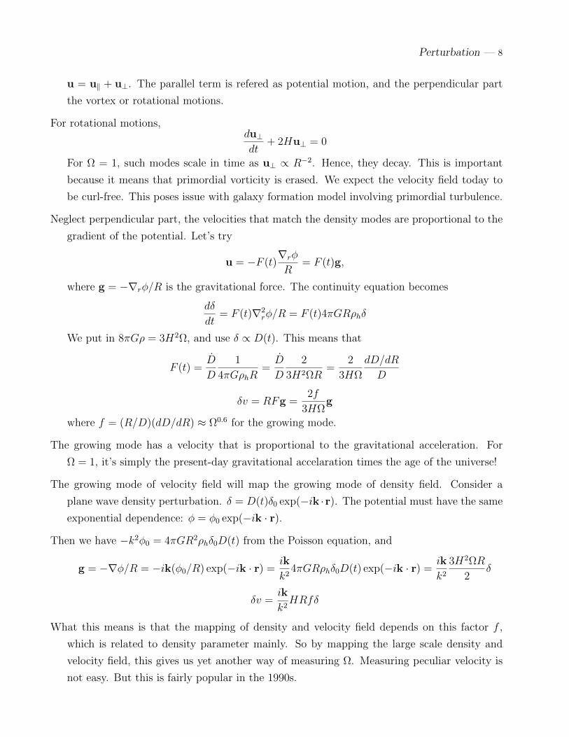
Perturbation — 8

u = u‖ + u⊥. The parallel term is refered as potential motion, and the perpendicular part

the vortex or rotational motions.

For rotational motions,du⊥dt

+ 2Hu⊥ = 0

For Ω = 1, such modes scale in time as u⊥ ∝ R−2. Hence, they decay. This is important

because it means that primordial vorticity is erased. We expect the velocity field today to

be curl-free. This poses issue with galaxy formation model involving primordial turbulence.

Neglect perpendicular part, the velocities that match the density modes are proportional to the

gradient of the potential. Let’s try

u = −F (t)∇rφ

R= F (t)g,

where g = −∇rφ/R is the gravitational force. The continuity equation becomes

dδ

dt= F (t)∇2

rφ/R = F (t)4πGRρhδ

We put in 8πGρ = 3H2Ω, and use δ ∝ D(t). This means that

F (t) =D

D

1

4πGρhR=D

D

2

3H2ΩR=

2

3HΩ

dD/dR

D

δv = RFg =2f

3HΩg

where f = (R/D)(dD/dR) ≈ Ω0.6 for the growing mode.

The growing mode has a velocity that is proportional to the gravitational acceleration. For

Ω = 1, it’s simply the present-day gravitational accelaration times the age of the universe!

The growing mode of velocity field will map the growing mode of density field. Consider a

plane wave density perturbation. δ = D(t)δ0 exp(−ik ·r). The potential must have the same

exponential dependence: φ = φ0 exp(−ik · r).

Then we have −k2φ0 = 4πGR2ρhδ0D(t) from the Poisson equation, and

g = −∇φ/R = −ik(φ0/R) exp(−ik · r) =ik

k24πGRρhδ0D(t) exp(−ik · r) =

ik

k23H2ΩR

2δ

δv =ik

k2HRfδ

What this means is that the mapping of density and velocity field depends on this factor f ,

which is related to density parameter mainly. So by mapping the large scale density and

velocity field, this gives us yet another way of measuring Ω. Measuring peculiar velocity is

not easy. But this is fairly popular in the 1990s.

Perturbation — 9

5 Non-linear perturbations

So far we’ve described the evolution of small perturbations. However, this is certainly not

the whole story.

When overdensities become non-linear (δ ≈ 1), the linear approximation does not break grace-

fully. Gravity is an attractive force, and the overdensities quickly run away to very large

density!

Higher-order perturbation theory is generally a very poor approximation in cosmology. We

quickly reach a regime of δ 1.

Numerical simulations show that the matter accumulates in dense regions. We call these regions

halos, because of our expectation that they correspond to the dark matter halos of galaxies

and clusters.

What stops the density from going to infinity? Random motions of the particles. As the particles

enter the dense region from various directions, they interpenetrate (the gas shocks). This

produces an effective pressure term that opposes further collapse.

Simulations and analytic models suggest that collapse is halted at an average overdensity of

about 200. The interior of the halos have higher densities, but it’s not because of cosmological

infall.

An important aspect of gravitational collapse is that non-linear collapse on small scales does

not spoil the linear evolution of large-scale perturbations. These perturbations don’t care

whether the matter on small scales is lumpy or not. Credit Gauss’s law!

Hence, in the non-linear regime, halos become our standard description.

Halos have different sizes and masses. They can merge together. There are models and simula-

tion results (that agree) to describe the mass functions and the merger rates.

Halos are viewed as the sites of galaxy and cluster formation. Hence, the formation of galaxy-

mass-sized halo is the precursor to the formation of luminous galaxies, while the merging of

those halos is the precursor to galaxy merging and cluster formation. We’ll talk more about

this later on.

One cannot solve the gravitational collapse problem from arbitrary initial conditions in the non-

linear regime. There are some analytic models (some of which have been remarkably useful),

but the primary workhorse here are numerical simulations.

Perturbation — 10

In the simplest form, one represents the cosmological density field by millions of particles and

then follows the motions of these particles according to their self-gravity. At the initial time,

the particles are nearly on a grid, but have been either displaced in position or in mass

to install some small perturbations, randomly generated to mimic the linear regime power

spectrum of the chosen cosmological model.

The particles generically clump into halos and one can study the inner properties and the

external correlations of these halos.

However, comparing to the real world requires building some statistics, so this is what we’ll talk

about next!

We wrote down hydro equations in our homogeneous comoving units, and rewrote it in perturba-

tive quantities. Then we linearlized it for small perturbations, which is appropriate for large

scale structure studies, and studied the properties of waves in this framework. We found

that for a non-expansing universe, we rediscovered Jeans instability, that is, when at long

wavelength or large scale, the pressure support can no longer balance gravity, or when free-

fall timescale is faster than sound-crossing timescale, gas will collapse and perturbation will

grow exponentially. Then we discussed that in an expanding universe, these perturbations

will not grow exponentially because the density of the universe is decreasing; they will grow

or decay as a power law. In a critical universe, the growth will be proportional to the overall

universe growth factor. We also briefly discussed the growth of peculiar velocities. The goal

of our studies is to (1) describe the large scale non-uniformity, or LSS, of the universe; (2)

understand the initial conditions, and the evolution of LSS, which teach us about cosmology.

In order to do that, we need to: (1) develop the statistical tools; (2) to study how different

initial condition will result in different statistical properties of LSS.

6 Non-linear perturbations

So far we’ve described the evolution of small perturbations. However, this is certainly not

the whole story.

When overdensities become non-linear (δ ≈ 1), the linear approximation does not break grace-

fully. Gravity is an attractive force, and the overdensities quickly run away to very large

density!

Higher-order perturbation theory is generally a very poor approximation in cosmology. We

quickly reach a regime of δ 1.

Perturbation — 11

Numerical simulations show that the matter accumulates in dense regions. We call these regions

halos, because of our expectation that they correspond to the dark matter halos of galaxies

and clusters.

What stops the density from going to infinity? Random motions of the particles. As the particles

enter the dense region from various directions, they interpenetrate (the gas shocks). This

produces an effective pressure term that opposes further collapse.

Simulations and analytic models suggest that collapse is halted at an average overdensity of

about 200. The interior of the halos have higher densities, but it’s not because of cosmological

infall.

An important aspect of gravitational collapse is that non-linear collapse on small scales does

not spoil the linear evolution of large-scale perturbations. These perturbations don’t care

whether the matter on small scales is lumpy or not. Credit Gauss’s law!

Hence, in the non-linear regime, halos become our standard description.

Halos have different sizes and masses. They can merge together. There are models and simula-

tion results (that agree) to describe the mass functions and the merger rates.

Halos are viewed as the sites of galaxy and cluster formation. Hence, the formation of galaxy-

mass-sized halo is the precursor to the formation of luminous galaxies, while the merging of

those halos is the precursor to galaxy merging and cluster formation. We’ll talk more about

this later on.

One cannot solve the gravitational collapse problem from arbitrary initial conditions in the non-

linear regime. There are some analytic models (some of which have been remarkably useful),

but the primary workhorse here are numerical simulations.

In the simplest form, one represents the cosmological density field by millions of particles and

then follows the motions of these particles according to their self-gravity. At the initial time,

the particles are nearly on a grid, but have been either displaced in position or in mass

to install some small perturbations, randomly generated to mimic the linear regime power

spectrum of the chosen cosmological model.

The particles generically clump into halos and one can study the inner properties and the

external correlations of these halos.

However, comparing to the real world requires building some statistics, so this is what we’ll talk

about next!

Perturbation — 12

Lets first develop statistical tools.

CfA redshift survey and SDSS survey plots.

7 Correlation Function

From these redshift surveys we know that galaxies are clustered. So how do we describe

the clustering mathematically. Here I am going to introduce two very important statistics.

Correlation function, and power spectrum.

One way to describe the tendency that galaxies like to stay together is the two point correlation

function ξ(r). Correlation functions ξ(r) is the excess probability that a galaxy is found at

a distance r from a known one. Hence,

ξ(r) =

⟨ρ(x + r)ρ(x)

ρ20

⟩− 1 = 〈δ(x + r)δ(x)〉

Here δ(r) is the density fluctuation field of galaxies in the universe

δ(x) =ρ(x)− ρ0

ρ0.

It is the density contrast to the random density. You might have thought the argument

should be a vector, but the claim is that the universe is statistically isotropic.

This idea of a correlation function can be extended to triplets and so forth. These are called

higher-order correlation functions. Note that these depend on the geometry of the locations,

so the vector directions of the separations now matter.

The other way to put it: let us have two small volumes ∆V1 and ∆V2, separated by distance

of r. The average spatial density of galaxies is ρ. Then the number of galaxies in ∆V1 is

ρ∆V1. Since ρ and ∆V are small numbers, it means that the chance of finding a galaxy in

∆V1 is ∆P1 = ρ∆V1. Now if galaxies are truly randomly distributed, then the chance of find

a galaxy in ∆V2 is ∆P2 = ρ∆V2. So the chance of finding a galaxy in both ∆V1 and ∆V2 is

∆P = ρ2∆V1∆V2.

In this case, galaxy distribution is uncorrelated. If galaxies are clustered, or correlated, then

the chance of finding a galaxy in ∆V1 and at the same time in ∆V2 is bigger than random:

∆P = ρ2∆V1∆V2(1 + ξ(r)).

So ξ(r) describes how much the two volumes, separated by r, are correlated, or how strong

the galaxies are clustered. If ξ(r) > 0, they are clustered. If ξ(r) < 0, they are anti-clustered,

Perturbation — 13

in other words, they tend to avoid each other. Clearly, in order to compute ξ(r), we need to

measure redshift in order to derive the real space distance. Also clear is that ξ is a function

of distance separation. At very large distance separation, the galaxy distribution will have

nothing to do with each other, so ξ(r) → 0 when r → ∞. On the other hand, if galaxies

are clustered, then the closer the separation is, the higher the possibility of finding a galaxy

next to a known galaxy is, comparing to the random field. When r → 0, this probability is

going to go to 1, or ξ(r)→∞. From observations, people find that it is a very good power

law:

ξ(r) = (r/r0)−γ.

Here r0 is called the correlation length, the scale at which the correlation function is 1, or

the probability of finding a galaxy from a known galaxy at a distance r is twice as high as

finding a galaxy in the random field. It is a very important parameter to measure in galaxy

surveys. At a few times r0, the galaxy distribution becomes to be very close to random.

Most galaxy redshift survey shows that r0 ∼ 5/hMpc and γ ∼ 1.8.

8 Power Spectrum

A common reformulation of these ideas is to study the density field in Fourier space. First,

we Fourier transform

δk =∫d3x δ(x)eik·x

and then we consider the statistical properties of the Fourier coefficients (which are complex

numbers).

The translational invariance of the statistical distribution gives useful properties. In particular,⟨δk⟩

= 0.

The most common statistic in Fourier space is the power spectrum. This is the two-point

correlations of the Fourier coefficients. In particular, we have⟨δkδ∗k′

⟩= (2π)3δ3D(k− k′)P (k)

δ3D(k− k′)is the Dirac delta function.

The power spectrum and correlation function are really just two representations of the same

information. In fact, the two functions are 3-d Fourier transforms of one another.

δ(x) =∫ d3k

(2π)3δke−ik·x

Perturbation — 14

ξ(r) = 〈δ(r)δ(0)〉 = 〈δ(r)δ(0)∗〉 =

⟨∫ d3k

(2π)3δke−ik·x

∫ d3k′

(2π)3δ∗k′

⟩

=∫ d3k

(2π)3

∫ d3k′

(2π)3e−ik·x 〈δkδ∗k′〉 =

∫ d3k

(2π)3

∫ d3k′

(2π)3e−ik·x(2π)3δ3D(k−k′)P (k) =

∫ d3k

(2π)3e−ik·xP (k)

While power spectrum and correlation function are basically the same thing, they are measured

in quite different ways, one by counting galaxy pairs, the other by deriving the density field

and its Fourier transform. They have different error properties and can have pros and cons

each in real life measurements.

What is a power spectrum, really? It’s the mean square amplitude of perturbations of a given

wavenumber. Since we found that each Fourier mode evolves independently in linear theory,

power spectra are particularly useful on linear scales.

A useful quantity to compute is the rms density fluctuation in a sphere of radius R. To do this,

first write that the density fluctuation in the sphere is

∆R =3

4πR3

∫sphere

d3r δ(r)

This has

〈∆R〉 =3

4πR3

∫sphere

d3r 〈δ(r)〉 = 0

The rms is then σ(R) = 〈∆2R〉

1/2.

For notational simplicity, let W (r) = 1 if the point is inside the sphere and W (r) = 0 otherwise.

W is called the window function. This special case is called a top-hat window. Then

σ2(R) =⟨∆2R

⟩=⟨

1

V

∫d3r δ(r)W (r)

1

V

∫d3r′ δ(r′)∗W (r′)

⟩=

1

V 2

∫d3r d3r′ W (r)W (r′)ξ(|r−r′|))

Without going through a few lines of simple but long math that deal with changing integrals

in Fourier transformation, we will get a simple one dimensional integral

σ2(R) =∫ d3k

(2π)3P (k)

|Wk|2

V 2

where Wk is the Fourier transform of our window function.

For our spherical window, the Fourier transform is also spherical. In detail, we have

Wk =∫d3r W (r)e−ik·r = V

3kR cos(kR)− 3 sin(kR)

(kR)3= V 3j1(kR)/(kR)

So, all together we have a simple one dimensional integral

σ2(R) =∫ ∞0

k2 dk

2π2P (k)

(3kR cos(kR)− 3 sin(kR)

(kR)3

)2

=∫ dk

k

k3P (k)

2π2w2(kR)

Perturbation — 15

Today, the rms fluctuation in spheres of 8h−1 Mpc radius is roughly 1. This corresponds to

masses of about 2× 1014h−1 M, which not coincidentally is the typical cluster mass. This

is yet another fundamental cosmological parameter: σ8.

Note that transforming between power spectrum, which tells you the amplitude of fluctuations

in different Fourier modes, and measured density fluctuation, involves details of your window

function. In observations, this window function is the geometry of your survey, including

both angular shape and vertical completeness as a function of redshift. Deriving power spec-

trum, which is what we really care as a physical quantity to be compared with theoretical

predications from the real observations requires one to understand the survey window func-

tion and model it carefully. And ideally, you want to design your survey to have as simple

window function as possible. But it is almost never possible to have a volume limited survey

with a top-hat window function.

It is important to note that the contribution to σ goes as∫ dk

kk3P (k). This means that P (k)

is not the appropriate quantity to base one’s intuition on where fluctuation power is coming

from. Rather, it is useful to think in terms of logarithmic intervals, in which case k3P (k) is

the relevant quantity. Basically, P is the fluctuation per point in k space, but the number

of points in k that contribute to the fluctuations scales as k3.

Indeed, it is increasingly popular to define ∆2(k) = k3P (k)/2π2 as the power spectrum (I call

it the dimensionless power spectrum). We then have σ2 =∫ dk

k∆2(k)|Wk|2.

Window functions are defined to have Wk=0 = 1, and they then usually cut off at some par-

ticular k. For most power spectra of interest, ∆2 is increasing with k, and so it is a rough

approximation that σ2 ≈ ∆2 where the latter is evaluated at the the cutoff scale of W , or

σ2 ≈ ∆2(1/R).

But one important issue in cosmology is that galaxies may or may not trace mass because of

the presence of dark matter. And in cosmology we mostly care about matter. So the real

parameter we concern about, and the parameter that theory is going to tell us, the the mass

fluctuation σ8(mass). It may or may not be one. And the ratio of the fluctuation in the

counts of galaxies to the fluctuation of underlying mass distribution is called the bias factor:

b =σ8(galaxies)

σ8(mass).

Since we know σ8(gal) = 1, to determine bias factor is the same as to determine σ8(mass), or

to determine the normalization of the mass power spectrum. A lot of effort in galaxy survey

business is to determine both the shape and the normalization of galaxy power spectrum,

and compare them with simulations, to constrain both cosmological parameters, as well as

Perturbation — 16

different flavors of dark matter models, in particular the thermal properties of dark matter

particles.

9 Types of dark matter

We know that most matter in the universe is dark matter. Let us first recall the reasons for

talking about dark matter, in particular non-baryonic dark matter, seriously in the context

of galaxy formation.

There are mostly three lines of evidence:

(1) the mass to light ratio in the MW, in galaxies, and in cluster of galaxies is much to high

for normal stellar population, in other words, the dynamical mass of a stellar system bigger

than globular cluster is always much bigger than stellar mass. So there must be missing, or

dark, matter.

(2) the determination of cosmological parameters should that Ωm ∼ 0.3, and from BBN, Ωb <

0.05, so there must be non-baryonic dark matter.

(3) a purely baryonic model of galaxy formation could not fit CMB data, nor could it generate

the structure that we see today.

So most people believe that the mass of the universe is dominated by non-baryonic dark matter,

i.e. mass in forms other than quarks, which makes protons and neutrons.

There are two flavors of DM people are still considering:

1. Hot dark matter. These are particles that decouple from the rest of the universe when it was

relativistic, and which have a number density roughly equal to that of photons. In this case,

there rest energy is a few eV, particular, few ev-mass neutrinos. Why we call them ”hot”?

For neutrinos with T = 1.95K today (neutrino background), their velocity is going to be:

v = 158(m/eV )−1km s−1. So the thermal velocity is very high, and it is even higher at high

redshift, this leads major effects on the development of self-gravitating structures.

2. Cold dark matter. It the particles decouple while they are nonrelativistic, there thermal

velocity today is effectively zero, and thus ”cold”. The typical candidates are WIMPS, or

weak-interacting massive particles, with possible mass of a few GeV.

One of the key considerations for theories of structure formation in which non-baryonic dark

matter dominant, is the damping of density perturbation by free-streaming. So long as the

DM particles are strongly coupled, they behave no different from ordinary particles. At later

Perturbation — 17

epochs, however, DM particles no longer interact with other particles. If the particle were

relativistic at the froze-out tome, they would continue to travel in straight lines at the speed

of light. Thus, if the particles belonged to some density perturbation, as they continue to

travel freely, they are going to damped out, or reduce the density fluctutation. The masses

which are damped out depend upon how far the free-streaming particles can traevel at a

given epoch. The comoving distance which a free-streaming particle can travel by epoch t is

just:

rFS =∫ t

0v(t)/R(t)dt.

Note that before the decoupling, the particle has the speed of light; however, after the

decoupling the particle will start to cool down as its speed will slow down with 1/(1 + z).

Taking this into account, one find that the mass scale of free-streaming damping is:

MFS = 4× 1015(m/30eV )−2M.

Therefore, if the hot dark matter neutrino mass is 30 eV, all density perturbations on mass

scale less than this will be damped out as soon as they come through the horizon. Since

these masses are of the order of massive clusters, in this picture, then, only structures at

larger scales can survive. There will be no or little power in the mass power spectrum at

smaller scales. So in hot dark matter cosmology, you have to make very large structure, the

so-called ”zeldovich pancake” first, and then the pancake will break down to make small

structure. This scenario is called the ”top-down” structure formation.

On the other hand, in the cold dark matter scenario, the CDM particles decoupled early in

the universe, after they had become non-relativistic. Free-streaming is unimportant. So in

CDM model, all the initial perturbations are preserved. THe CDM model is the popular,

and working model of structure formation.

The CDM model can be studied using computer simulations in great detail, once the initial

power spectrum of fluctuation is given. As I will show you in a moment, these spectra are

such that there is most power on the small scale, so the lowest mass objects form first. These

then undergo hierarchical clustering under the influence of perturbations on large scales and

so the larger scale, which has smaller initial perturbation, and therefore takes longer time to

grow, are built-up later. This bottom-up, or hierarchical structure formation is the base of

all the galaxy formation theory today.

Perturbation — 18

10 Primordial power spectrum

The density fluctuation power spectrum of the universe consists of two parts: the primordial

power spectrum, which is power spectrum the universe began with, and the effect that

happens on top of that after the scale in question has entered the horizon as the universe

is expanding. The function that describes the changes to the input initial spectrum of the

perturbation is called the transfer function.

The initial power spectrum is typically described as having a power-law form:

P (k) ∼ kn.

Let’s call the density fluctuation at mass scale M to be σ(M), one can show (find proof in

Longair) that: σ(M) ∼ M−(n+3)/6, so as long as n > −3, the mass fluctuation decreases to

large mass scales. This is good. We want the universe to be uniform on large scales.

The n = 1 case is of special interests. This spectrum has the property that the density fluctuation

σ(M) had the same amplitude on all scales when the perturbations came through the horizon.

It is useful to look at the density perturbation of a certain size/mass scale at the time it

enters the particle horizon r = rH = ct where t is the age of the universe at a certain time.

We mentioned before that in radiation dominated era, the perturbation grows as δ ∼ R2.

So the fluctuation grows and changes with horizon mass scale as:

σ(MH) ∼ R2M−(n+3)/6H .

And the horizon mass scale is MH ∼ ρDt3. In radiation dominated era: R ∼ t1/2, ρ ∼ R−3,

so MH ∼ R3. Plug all these things in, you will find:

σ(MH) ∼M2/3M−(n+3)/6.

And if n = 1, the amplitudes of the density perturbation were all the same when the came

through their particle horizons during the radiation dominated era.

This particular form of primordial power spectrum is called the Harrison-Zeldovich spectrum,

first suggested by Harrison and Zeldovich, independently, in early 1970s. It has a number of

very appealing features. In particular, if n = 1, then the universe is fractal, or self-similar,

in the sense that every perturbation came through the horizon with the same amplitude,

and as the universe expands, we always find perturbations of the same amplitude appearing

on the horizon; the universe looks the same when viewed on the scale of the horizon. It is

simple, and it occurs very naturally in inflationary models. It is sometimes also called the

scale-invariant spectrum. Deviations of the power-law exponent from this special value are

Perturbation — 19

known as ‘tilts’. Modern measurements find that n is rather close to 1, e.g., WMAP finds

that n = 0.99 ∼ 0.04.

Transfer function, or the effect on the perturbation power spectrum after it has entered horizon.

The transfer function T(k) describes how the shape of the initial power spectrum in the dark

matter is modified by different physical processes:

∆k(z = 0) = T (z)D(z)∆k(z)

Here D(z) is the growth function we discussed before D(t) ∝ 1/(1 + z) for critical universe.

There are two effects that I want to mention:

(1) the free-streaming effect that we just talked about. This will reduce the small scale power in

hot DM models because the gravitationally important neutrinos are free-streaming around

and damped the fluctuation.

(2) effect related to pressure in radiation dominated era. In the matter-dominated era, all scales

grow equally. However, in the radiation-dominated era, things behave differently. Here,

pressure is important; indeed, the sound speed is c/√

3! Remember that in the previous

derivation of growth function, we ignored the sound speed and pressure term by assuming

CDM. But it does matter in early times due to coupling. On scales smaller than the horizon,

the growth is stalled by the presence of the radiation pressure. Basically, the universe expands

too quickly for the dark matter to collapse. So on small scales the radiation remains smooth,

but on large scales it has to cluster. So, scales that enter the horizon (i.e. suffer from smooth

radiation) during the radiation-dominated epoch grow less than those that enter the horizon

during the matter-dominated epoch. As soon as the perturbations came through the horizon,

they cease to grow until the epoch of equality, after which they grow as described in the

growth function.

One thing we didn’t do is to work out the growth of perturbation in radiation dominated era.

Going through the same process as we did before, one can show that in radiation dominated

era,

∆ ∝ t ∝ (1 + z)−2.

Thus, for the small scale (large k) which enters horizon early, ∆ will not grow and suppressed

by a factor of (RH/Req)2, or by a factor of k2. Therefore, the power spectrum itself will be

suppressed by a factor of k4 on small scale or large k. The transition happens at the horizon

size of matter/radiation equality, which is about 100 Mpc co-moving.

This effect results in that the density fluctuation σ(M) ∼ M−(n+3)/6 is roughly flat on small

scales. So the processed power spectrum will have P (k) ∼ k−3 on small scales, P ∝ k on

Perturbation — 20

large scales, the scale of the horizon at matter-radiation equality, which is about 100 Mpc

for LCDM model in comoving units.

11 Power spectra in different cosmologies

Figure.

I want to draw your attention to five particular models: cold dark matter, hot dark matter,

and mixed, or C+H dark matter, LCDM, and TCDM, or titled CDM model. CDM refers to

models with massive DM, such as WIMPs or weak interacting massive particles. They are

typically very massive, like GeV level, and have practically zero velocity. They are the kind

of model whose power spectra fits the data. SCDM model is the most standard, self-similar

model, with Ω = 1, and a CDM power spectrum with initial H-Z spectrum. We know that

observations have more or less ruled it out. TCDM model is the CDM model with a tilted,

or n 6= 1 power spectrum. This model sometimes produces a better fit than SCDM when

choosing proper tilt. But it still has Ω = 1, so out. LCDM model is the working hypothesis

in cosmology. HDM refers to models with relatively light DM particles, in particular with

mass around 100 eV, possible for mass of neutrinos. They could have mass dominating the

universe, and they are light weighted, and therefore have relativistic speed. So you can think

of them as free streaming. Because of the free streaming and their dominance in mass, they

will tend to wash out any perturbation on scales comparable to the horizon size when first

galaxy formed, or at small scales. So these models all have very strong cut off on power

spectra on large k, or small R. They are totally inconsistent with observations now, and

nobody discussed them seriously anymore. Some version of mixed dark matter model, in

which both cold, WIMPS, and hot, neutrinos, contribute the DM, were still popular until

recently, although they appear to be as very ugly.

One of the important goals of redshift survey is to use the power spectrum to constrain these

DM models, as we see, it is certainly very useful and successful. But now, if we all buy the

LCDM model, as indicated by WMAP, then what exactly galaxy power spectrum tells you?

In my view, it now tells you more about galaxies than about cosmology. In other words,

our key assumption, which I didn’t quite make explicit, is that galaxies trace mass, except

for a constant bias factor. This is a big assumption. To the first order, it is true because

at very large scale that we care about, baryonic process in addition to pure gravity is not

important. But it is not completely negligible, otherwise, we won’t have our morphology-

density relation, which says that galaxies do care about the environment they live in. So

Perturbation — 21

now by studying the LSS, we will actually learn a lot about how galaxy form and evolve, if

we assume we know the underlying cosmology, by looking at how bias factor change with

scale or galaxy type.

12 Observations of large scale structure

As we look out into the sky, it is quite clear that galaxies are not spread uniformly through

space. They are clumped into groups, which consist of tens of galaxies, clusters, with hun-

dreds of galaxies, and superclusters etc. Galaxies are clustered, in order words, galaxies

like to stay together. The possibility of finding a galaxy next to another galaxy is much

higher than the possbility of finding a galaxy next to an empty spot on the sky. We call this

non-uniform distribution of galaxies in space the large scale structure of the universe. Large,

here, refers to scales of at least 10Mpc, i.e., larger than the scale of a cluster of galaxy, which

is few Mpc.

The primary observational tool to study the large scale structure of galaxies is galaxy redshift

survey. The goal of galaxy redshift survey is to study the statistical properties of galaxy

population over a large volume. Therefore, to carry out statistical studies, we need a well-

defined survey, such as a flux-limited survey, simply getting a lot of galaxy redshift is not

enough, statistical completeness is the key; of course, to sample a large volume, we need to

measure the redshift of many, many galaxies, over a large fraction of the sky.

There are different flavors of redshift surveys: one-dimensional, or pencil-beam survey, which

goes deep over a very small area of the sky. This is especially useful to study galaxy evolution.

two-dimensional, or slice survey, in which a long, thin strip on the sky is covered.

three-dimensional survey, in which a substantial solid angle on the sky is covered. This is the

best way, but also the most expensive way to do it.

A bit of history. Large scale structure was recognized from two-D maps of the galaxy distribution

very early on, from the time of Hubble or even earlier. de Vaucouleurs recognized the

existence of the local Supercluster in the 1940s. One important event in large scale structure

was the publication of the deep galaxy count map based on photographic plates from Lick

Observatory in late 1960s, which enabled the first generation of statistical studies of galaxy

distribution. But this is still only two-D, in other words, it is the angular distribution, of

galaxies, not the spatial distribution. In order to get the radial direction, we need redshift.

Here obviously we are assuming that redshift is really proportional to distance. We will see

that it is not always true in just a little bit.

Perturbation — 22

To get redshift of course requires you to get spectrum, which is very time consuming. It was

very difficult to do until about 20 years ago. There were various attempts in late 1970s and

early 1980s. But the major breakthrough came in 1960s, when a team of astronomers at

CfA published the first slice of their redshift survey (figure). This striking figure shows that

the distribution of galaxies in space is obviously not random. In fact, it is very organized,

structured. This kind of figure is sometime called wedge diagram, or pie diagram, with

position (1-D) in one direction and redshift (distance) in the other. Ignoring peculiar velocity,

the velocity component deviates from uniform Hubble flow, then this figure takes us to 14,000

km/s, or if we assume H of 70, 200 Mpc in distance.

This is one of the most important figures in extragalactic astronomy. The CfA survey made all

the headlines, and really put the study of large scale structure of galaxies at the center of

astronomical research for more than a decade. In late 80s to early 90s, when I was a undergrad

and beginning grad student, everything people talked about was redshift surveys. Because,

as we will see, the distribution of galaxies contains important clues to the properties of the

universe, in particular it is related to the mass density, and to the nature of dark matter.

Now we can probably measure these better with CMB, and the maybe we are nearing to the

end of the golden age of redshift survey. But it is still one of the most important areas in

cosmology.

From this figure, we can learn a number of terms that people uses in LSS. Great wall. It

originally refers to this particular structure at about 7000 km/s, or 70/h Mpc away in the

CfA survey. Void, between filaments we find large regions that are almost empty of bright

galaxies; these voids are typically 50Mpc or larger. Finger of God. This particular structure

here is in the direction of Coma cluster, the nearest rich cluster of galaxies. Coma in this

redshift figure is not shown as a roundish structure, but a very elongated finger, covering

about 3000 km/s, or about 30/h Mpc. But we just said that cluster is few Mpc across. What

went wrong?

The key is that we were assuming that the universe was expanding uniformly, that the redshift is

exactly proportional to distance and there no peculiar velocity. This is not true, in particular

for a rich cluster of galaxies, where the velocity dispersion is of the order 1000 km/s. So the

redshift of the galaxy here that belongs to Coma is a combination of cosmological redshift and

peculiar velocity due to the gravitational pull from Coma itself. This particular pheonomenon

that peculiar velocity increases near a massive object, resulting in this kind of elongated

structure in redshift dimension is called the finger of God.

As I said, redshift survey, and the studies of LSS, have been the center of extragalactic astronomy

Perturbation — 23

for the past 30 years. Especially after the CfA survey, a great amount of efforts have been put

into carrying out even larger, deeper, and better redshift surveys, using new technology and

larger telescopes. Just to mention a few, the original CfA survey has 2417 galaxies down to

14.5 mag, the Las Campanas redshift survey in mid 1990s had about 80000 galaxies, the 2dF

survey recently finished has 250,000 galaxies, and the ongoing SDSS will have one million

galaxies. These are currently the largest redshift survey. People are also pushing towards

higher redshift, with 8-10m class telescope. The earliest one was one carried out at Keck,

which will produce about 15,000 redshifts at z ∼ 0.7 − 1.3. These are very faint galaxies,

and the whole survey used 120 Keck nights.

The measurement of power spectra from galaxies and other cosmic structures have provided a

powerful probe to cosmology.

(1) the overall shape of power spectrum provide information on the initial power spectrum,

whether it is Harrison-Zeldovich, or tilted.

(2) The small scale shape shows that the perturbation is mostly from CDM. HDM has very

different shapes.

(3) The peak of power spectrum corresponds to the horizon scale of equality of mater and

radiation. This wave number is related to both the redshift of equality, and the size of the

universe at that time which is related to the expansion history. Turns out teq = 7.3×10−2Ω0h2

Mpc−1. Therefore, measurement of power spectrum directly measures Ω0h – the other factor

of h is absorbed in the distance dependence of Hubble constant.

(4) There are detailed difference between open and Λ dominated models, but they are subtle.

The power to determine Λ from LSS comes from combining with CMB which shows that the

universe is flat.

Tegmark plot. We will discuss the next generation of redshift surveys, including BOSS, eBOSS,

DESI, PFS, LSST, EUCLID and WFIRST, after talking about BAO in CMB lecture.