Lecture notes on Regression: Markov

Chain Monte Carlo (MCMC)

Dr. Veselina Kalinova, Max Planck Institute for Radioastronomy, Bonn

“Machine Learning course: the elegant way to extract

information from data”, 13-23 Ferbruary, 2017

March 1, 2017

1 Overview

Supervised Machine Learning (SML): having input variables (X) and outputvariables (Y), adopt an algorithm to understand the mapping function: Y=f(X).

Goal of SML: to find a function f(X), which can predict well the new outputvalues (Y’) for a given set of input values (X’).

• Regression problem: the output value is a real value, i.e., ”height” or”weight”

• Classification problem: the output value is a category, i.e., ”red” or ”blue”

2 Regression Analysis

2.1 Linear regression

Example: a) line-fitting

yi = �0 + �1xi + ✏i, (1)

where i=1,...,n is the particular observation; �0 and �1 - linear parameters,✏i - error.

b) parabola-fitting

yi = �0 + �1xi + �2x2i + ✏i, (2)

where i=1,...,n is the particular observation; �0, �1 and �2 - linear parame-ters, ✏i - error (still linear regression, because the coe�cients �0, �1 and �2 arelinear, although there is a quadratic expression of xi).

1

Figure 1: Linear Regression for a given data set x. left: line-fitting. Right:

parabola-fitting.

2.2 Ordinary least squares

We define the residual ei as the di↵erence between the value of the dependentvariables, predicted by the model yMOD

i and the true value of the dependentvariables, yOBS

i , i.e.,

ei = yOBSi � yMOD

i (3)

One way to estimate the residuals is through ”ordinary least squares” method,which minimaze the sum of the squared residuals (SSE):

SSE =X

i=1

ne2i (4)

The the mean square error of regression is calculated as

�2✏ = SSE/dof, (5)

where dof = (n � p) with n-number of observations, and p-number of pa-rameters or dof = (n� p� 1) if intersept is used.

2.3 Best fit of function

The best fit of a function is defined by the value of the ”chi-square”:

�2 =NX

i=1

[yOBSi � yMOD

i ]2

✏2yi

, (6)

where our data/observations are presented by yOBSi with error estimation

✏yi

, and model function yMODi .

It is aslo necessary to know the number of degrees of freedom of our model⌫ when we derive the �2 , where for n data points and p fit parameters, thenumber of degrees of freedom is ⌫ = n � p. Therefore, we define a reducedchi-square �2

⌫ as a chi-square per degree of freedom ⌫:

2

Figure 2: The minimum chi-square method aims to find the best fit of a function.left: for one parameter, right: for two parameters

�2⌫ = �2/⌫, (7)

where ⌫ = (n�m) with n - number of measurements, and p - number of fittedparameters.

• �2⌫ < 1 ! over-fitting of the data

• �2⌫ > 1 ! poor model fit

• �2⌫ ' 1 ! good match between data and model in accordance with the

data error

2.4 The minimum chi-squared method

Here the optimum model is the satisfactory fit with several degrees of freedom,and corresponds to the minimusation of the function (see Fig.2, left). It isoften used in astronomy when we do not have realistic estimations of the datauncertainties.

�2 =NX

i=1

(Oi � Ei)2

E2i

, (8)

where Oi - observed value, and Ei - expected value.If we have the �2 for two parameters, the best fit of the model can be

represented as a contour plot (see Fig.2, right):

3

3 Markov Chain Monte Carlo

3.1 Monte Carlo method (MC):

• Definition:”MC methods are computational algorithms that rely on repeated ran-dom sampling to obtain numerical results, i.e., using randomness to solveproblems that might be deterministic in principle”.

• History of MC:First ideas: G. Bu↵on (the ”needle experiment”, 18th century) and E.Fermi (neutron di↵usion, 1930 year)Modern application: Stanislaw Ulam and John von Neumann (1940),working on nuclear weapons projects at the Los Alamos National Labo-ratoryThe name ”Monte Carlo”: chosen as a secret name for the nuclearweapons projects of Ulam and Neumann; it is named after the casino”Monte Carlo” in Monaco, where the Ulam’s uncle used to play gamble.MC reflects the randomness of the sampling in obtaining results.

• Steps of MC:a) define a domain of possible inputsb) generate inputs randomly from a probability function over the domainc) perform deterministic computation on the inputs (one input - one out-put)d) aggregate (compile) the results

• Perfoming Monte Carlo simulation (see Fig.3):

Area of the triangle, At =12x

2

Area of the square, Abox = x2

Therefore, 12 = A

t

Abox

) Abox = 12At.

We can define the ratio between any figure inside the square box

by random sampling of values.

1630 ⇠ 1

2 by counting the randomly seeded points

12 ⇠ counts in triangle

counts in box

Monte Carlo algorithm is random - more random points we take,

better approximation we will get for the area of the triangle (or

for any other area imbeded in the square) !

4

Figure 3: Example for Monte Carlo simulation - random sampling of points(right) to find the surface of a triangle inside a square (left), i.e., the ratiobetween the counts of the points wihin the two regions will give us the ratio oftheir surfaces. Our estimation will be more accurate if we increase the numbersof the points for our simulation.

Figure 4: Representation of a Markov Chain.

3.1.1 Markov Chain

• First idea: Andrey Markov, 1877

• Definition: If a sequence of numbers follows the graphical model in Fig.4, it is a ”Markov Chain”. That is, the probability pi for a given value xi

for each step ”i”:

p(x5|x4, x3, x2, x1) = p(x5|x4) (9)

The probability of a certain state being reached depends only on the previ-

ous state of the chain!

• A descrete example for Markov Chain:We construct the Transition matrix T of the Markov Chain based on theprobabilities between the di↵erent state Xi, where i is the number of thechain state: 2

40 1 00 0.1 0.90.6 0.4 0

3

5

5

Figure 5: Markov Chain Monte Carlo analysis for one fitting parameter. Thereare two phases for each walker with an initial state: a) burn-in chain and b)posterior chain.

Let’s take a starting point X0 with initial probabilities X0 = (0.5, 0.2, 0.3).The next step X1 will evolve as X1 = X0 ⇥ T = (0.2, 0.6, 0.2) and thesystem will converge to Xconverged = (0.2, 0.4, 0.4).

Additional two conditions have to be applied in the evolution of the sys-tem, the chains have to be:a) Irreducible - for every state Xi, there is a positive probability of movingto any other state.b) Aperiodic - the chain must not get trapped in cycles.

• Phases of the Markov Chain (see Fig.5):

a) ”burn-in” chain - throwing some initial steps from our sampling, whichare not relevant and not close to the converging phase (e.g., we will removesome stuck walkers or remove ”bad” starting point, which may over-sampleregions with very low probabilities)

b) posterior chain - the distribution of unknown quantities treated as arandom variables conditional on the evidence obtain from an experiment,i.e. this is the chain after the burn-in phase, where the solution settles inan equalibrium distribution (the walkers oscillate around a certain value)

4 Bayes’ theorem

• First idea: Thomas Bayes, 1701-1761

6

• Importance: Bayes’s theorem is fundamental for Theory of Probabilityas the Pythagorean theorem for the Geometry.

• Definition: it can be expressed as the following equation of probabilityfunctions

P (A|B) =P (B|A)P (A)

P (B), (10)

where A and B are events, P (B) 6= 0.

- P (A) and P (B) are probabilities of observing event A and event B with-out regard to each other; P (A) is also called ”prior” probability, whileP (B) - ”evidence” or ”normalisation” probability- P (A|B) is a conditional probability, i.e., the probability of observingevent A given that the event B is true (or ”posterior” probability)- P (B|A) is a conditional probability, i.e., the probability of observingevent B given that the event A is true (or ”likelihood” probability)

• Example:We examine a group of people. The individual probability P (C) for eachmember of the group to have cancer is 1 %, i.e., P (C)=0.01. This is a”base rate” or ”prior” probability (before being inform for the particularcase). On the other hand, the probability of being 75 years old is 0.2 %.What is the probability as a 75 years old to have a cancer, i.e.,

P (C|75)=?

a) C - event ”having cancer” =) probability of having cancer is P (C) =0.01b) 75 - event ”being 75 years old” =) probability to be 75 years old isP (75) = 0.002c) the probability 75 years old to be diagnosed with cancer is 0.5 %, i.e.,P (75|C) = 0.005

P (C|75) = P (75|C)P (C)

P (75)=

0.005⇥ 0.01

0.002= 2.5%, (11)

(This can be interpreted as: in a sample of 100 000 people, 1000 will havecancer and 200 people will be 75 years old. From these 1000 people - only5 people will be 75 years old. Thus, of the 200 people, who are 75 yearsold, only 5 can be expected to have cancer.)

7

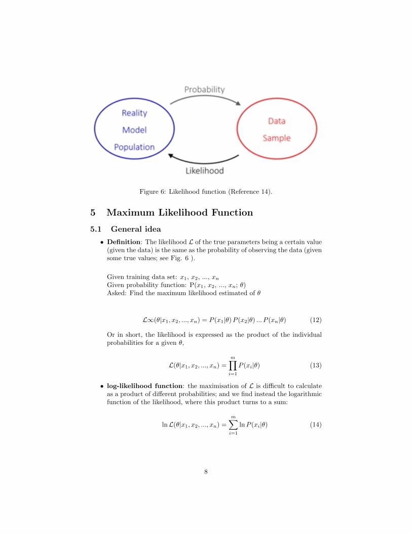
Figure 6: Likelihood function (Reference 14).

5 Maximum Likelihood Function

5.1 General idea

• Definition: The likelihood L of the true parameters being a certain value(given the data) is the same as the probability of observing the data (givensome true values; see Fig. 6 ).

Given training data set: x1, x2, ..., xn

Given probability function: P(x1, x2, ..., xn; ✓)Asked: Find the maximum likelihood estimated of ✓

L1(✓|x1, x2, ..., xn) = P (x1|✓)P (x2|✓) ... P (xn|✓) (12)

Or in short, the likelihood is expressed as the product of the individualprobabilities for a given ✓,

L(✓|x1, x2, ..., xn) =mY

i=1

P (xi|✓) (13)

• log-likelihood function: the maximisation of L is di�cult to calculateas a product of di↵erent probabilities; and we find instead the logarithmicfunction of the likelihood, where this product turns to a sum:

lnL(✓|x1, x2, ..., xn) =mX

i=1

lnP (xi|✓) (14)

8

Figure 7: Maximazing log-probability function.

a) maximaze log-probability functionWe need to find the maximum value of the log-probability function, correspond-ing to the optimum best-fit value of the function for a given parameter ✓. Thisis exactly the derivative of the lnL with repect to ✓ made equal to zero:

@ lnL(✓|x1, x2, ..., xn)

@✓= 0 (15)

b) verify log-probability function (see Fig. 7)To find the global maximum of the log-probability function,

@2 lnL(✓|x1, x2, ..., xn)

@✓< 0 (16)

5.2 Example 1:

Given samples 0,1,0,0,1 from a binomial distributionTheir probabilities are expressed as:P(x=0)=1-µP(x=0)=µ

Requested: What is the maximum likelihood estimated of µ?

Therefore, we define the likelihood as product of the individual probabilities:

L(µ|x1, x2, ..., xn) = P (x = 0)P (x = 1)P (x = 0)P (x = 0)P (x = 1) =

(1� µ)µ (1� µ) (1� µ)µ = µ2(1� µ)3 .(17)

Further, we find the log-likelihood function as

lnL = 3 ln(1� µ) + 2 lnµ. (18)

9

We find the maximum value of the log-probability function:

@ lnL@µ

= 0 (19)

) �3µ+ 2(1� µ) = 0 (20)

) µ =2

5(21)

Finally, we verify if we find the global maximum of the log-probability func-tion by the second order derivative:

@2 lnL@µ

=3(�1)

(1� µ)2� 2

µ2 0 (22)

Therefore, the value µ = 25 is indeed our maximum estimate of the log-

likelihood function.

5.3 Example 2:

Let’s find the likelihood function of data represented by a line in the formy = f(x) = mx + b, where any reason for the data to deviate from a linearrelation is an added o↵set in the y-direction. The error yi was drawn from aGaussian distribution with a zero mean and known variance �2

y.In this model, given an independent position xi, an uncertainty �y

i

, a slopem, an intercept b, the frequence distribution p is:

p(yi|xi,�yi

,m, b) =1q2⇡�2

yi

e� |y

i

�mx

i

�b|2

2�2y

i . (23)

Therefore, the likelihood will be expressed as:

L =NY

i=1

p(yi|xi,�yi

,m, b) ) (24)

lnL = K �NX

i=1

|yi �mxi � b|2

2�2yi

= K � 1

2�2, (25)

where K is some constant.Thus, the likelihood maximization is identical to �2

minimization !

10

6 Bayesian generalization

The Bayesian generalization of the frequency distribution p, described in equa-tion 23, have the following expression:

p(m, b|{yi}Ni=1, I) =p({yi}Ni=1|m, b, I) p(m, b|I)

p({yi}Ni=1|I), (26)

where m, b � model parameters{yi}Ni=1 � short-hand for all of the data yiI� short-hand for all the prior knowledge of the xi and �y

i

.

Further, we can read the contributors in equation 26 as the fol-

lowing:

p(m, b|{yi}Ni=1, I) ! Posterior distributionp({yi}Ni=1|m, b, I) ! Likelihood L distributionp(m, b|I) ! Prior distributionp({yi}Ni=1|I) ! Normalization constant

Or,

Posterior =Likelihood⇥ Prior

Normalization(27)

7 The Metropolis algorithm

• First ideas (in the modern time):

The algorithm is origially invented by Nicholas Metropolis (1915-1999),but generalized byWilfred Hastings (1930-2016), later it is called Metropolis-Hastings algorithm.

• Basic assumptions in the Metropolis algorithm:

- assumes a symmetric random walk for the proposed distribution, i.e.,q(x|y) = q(y|x)

- the posterior distribution is approximated to the Bayesian probabilitiessince the dominator term in equation 27 is di�cult to calculate in practice,but at the same time possible to ignore due to its normalization nature

- the walkers are keep jumping to explore the parameter space even if theyalready found the local minimum

- to improve the e�ciency in the MCMC algorithm, the burn-in chainsare removed

11

Figure 8: Burn-in and post burn-in steps (credit: Reference 12)

• Metropolis rules:

General Case Ignoring Priors Ignoring Priors& assuming Gaussian errors

if Ptrial > Pi if Ltrial > Li �2trial < �2

i

accept the jump, so accept the jump, so accept the jump, so✓i+1 = ✓trial ✓i+1 = ✓trial ✓i+1 = ✓trialif Ptrial < Pi if Ltrial < Li �2

trial > �2i

accept the jump with accept the jump with accept the jump withprobability Ptrial/Pi probability Ltrial/Li �2

trial/�2i

where P , L and �2 are the probability, likelihood and chi-squared distri-butions, repectively. Additionaly, with ✓ are expressed the positions ofthe walkers.

References

(1) Kalinova et al., 2017, MNRAS, 464, 1903 (http://adsabs.harvard.edu/abs/2017MNRAS.464.1903K)(2) http://vcla.stat.ucla.edu/old/MCMC/MCMC_tutorial.htm(3) http://www.mcmchandbook.net/HandbookChapter1.pdf(4) http://physics.ucsc.edu/~drip/133/ch4.pdf(5) https://ned.ipac.caltech.edu/level5/Wall2/Wal3_4.html(6) https://en.wikipedia.org/wiki/Regression_analysis

12

(7) https://en.wikipedia.org/wiki/Reduced_chi-squared_statistic(8) https://en.wikipedia.org/wiki/Markov_chain_Monte_Carlo(9) https://en.wikipedia.org/wiki/Bayes’_theorem(10) https://en.wikipedia.org/wiki/Maximum_likelihood_estimation(11) https://en.wikipedia.org/wiki/Metropolis%E2%80%93Hastings_algorithm

Videos:

(12) https://www.youtube.com/watch?v=vTUwEu53uzs(13) https://www.youtube.com/watch?v=h1NOS_wxgGg(14) https://www.youtube.com/watch?v=2vh98ful3_M(15) https://www.youtube.com/watch?v=BFHGIE-nwME(16) https://www.youtube.com/watch?v=AyBNnkYrSWY

13