lecture notes on propositional and predicate logic
TRANSCRIPT

Lecture Notes onPropositional andPredicate Logic
Martin PilátBased on lecture by Petr Gregor
january 2, 2019


Introduction
Generally, logic is a study of arguments and inferences. While it startedas philosophical discipline in ancient times, it is now widely studied inmathematics and computer science. As such, logic provides the basiclanguage and tools for most of mathematics. It studies different provesystems and discusses whether they are sound (everything they proveis valid) and complete (everything that is valid can be proven).
While logic provides rather low-level tools for mathematics andcomputer science, it still has rather wide applications. For example,in some areas of artificial intelligence, logic is used to represent theknowledge of the intelligent agents and reason about it. The agentsthen use logical reasoning (theorem proving) to decide what to donext, or prove that a certain action is safe in a given environment.Another important area is formal software verification, where logic(and, again, theorem proving) can be used to formally verify, that aprogram indeed does what it should according to a specification. Thisis essential while implementing e.g. cryptographic protocols. Formalverification is also used while designing digital circuits.
There are also attempts to formalize the whole mathematics in logicand use computers to check that all the proofs are correct. For example,Mizar1 is a system that aims to re-create most of the mathematics with 1 http://www.mizar.org/library/
formal and verified proofs. The verification starts from the basicmathematical axioms – in the case of the Mizar system, authors of socalled Mizar articles can use only axioms of set-theory and theoremsfrom previously verified articles. Therefore, everything published inthe Mizar mathematical library is verified to be a correct consequenceof the base axioms.
Logic serves as the formal language of mathematics, and thereforelogic also needs to formally specify the syntax of the language. Thesyntax defines, what is a valid logical formula and what is not, how-ever the meaning and validity of a formula is given by the semanticsof the language. Logic itself prescribes the meaning of only a handfulof symbols – namely the logical connectives (∧,∨,→,↔,¬) and thequantifiers (∀, ∃). Additionally, in languages with equality, the mean-ing of “=” is also given. All other symbols used in logical formulascan have arbitrary meaning, which is given by the semantics. So, forexample, if we write a formula (∀x)(∀y)(x + y = y + x), we cannotdiscuss its validity before defining the meaning of “+”. The formulais valid if we are talking about the real numbers and “+” denotestheir addition, however, the symbol “+” can also represent (quite un-

4 LECTURE NOTES ON PROPOSITIONAL AND PREDICATE LOGIC
usually) the multiplication of square matrices, and in such a case, theformula is not valid.
There are different levels of the language of logic. In propositionallogic, only propositional variables (those that are either true or false)and the logical connectives can be used. In first order logic, we canadditionally use functions, relations and quantifiers for variables thatrange objects from some universe. In second order logic, there areadditionally quantifiers for sets of objects in the universe (and, morespecifically, for functions and relations). In higher order logic, we alsohave variables for sets of sets of objects. For example, a formula inpropositional logic
(d ∧ c)→ s
can express that if it is dark and clear outside, the stars are visible. In afirst order language, we can have a more complex formula
(∀x)(∀y)(S(x) ∧ E(y)→ (L(x, y)→ P(x, y)))
that expresses that if x is a student (S(x)) and y is an exam (E(y)), if xlearns for y (L(x, y)) then x passes y (P(x, y)). As an example of secondorder language, we can write the axiom of induction:
(∀P)(P(0) ∧ (∀n)(P(n)→ P(n + 1))→ (∀n)P(n)) .
In the lecture, we will deal mostly with propositional and first-orderlogic, however there are also other extension of logic. For example, inmulti-agent systems, so called modal logic is often used to representthe knowledge. In modal logic, there are special modalities, that canfurther qualify a statement. For example, there is a modality that saysthat a statement may be true, or must be true. Other types of modallogic contain modalities that express knowledge of other agents (e.g.“agent A knows that statement S is true” can be written as KA.S, oreven “agent A knows that agent B knows that statement S is true”(KA.KB.S)). Another interesting type of modal logic is temporal logic,which contain modalities about time and can express e.g. “statementS will be true sometimes in the future”.
About these lecture notes
In these lecture notes, logic is presented for students of computer sci-ence. Therefore, focus is given to areas most needed for computerscientists. For example, we use the more intuitive tableau method in-stead of the Hilbert-style prove systems. We also explain the resolutionmethod in logic as a background to Prolog and logical programming.The more advanced topics on decidability and incompleteness areexplained in a more informal way.
You are currently reading the first version of the lecture notes, whichcan, and most probably will, contain some errors. If you find an error,or if something is not clear, do not hesitate to contact the author bye-mail2, or, alternatively, create an issue in the GitHub repository of 2 [email protected]
the book3. 3 https://github.com/martinpilat/
logic-book

INTRODUCTION 5
There are also other resources you may want to check. One of themare the presentations created by Petr Gregor for his version of thelecture4, that serve as a base for these lecture notes. 4 http://ktiml.mff.cuni.cz/~gregor/
logics/index.htmlInformal! The author of these notes sometimes likes to explainthings in a more intuitive way with some not-so-formal examplesand metaphors. While he believes these can help to get better un-derstanding of the given concept, they sometimes (read “often”) arerather informal and have some limitations. Therefore, in these notes,they will be set in boxes like the one you are reading just now with abold “Informal!” warning. The information contained in these boxesis always non-essential to the rest of the text and can be (some wouldeven argue that should be) skipped.
Preliminaries
Like many mathematical texts, these lecture notes also assume thatthe reader has some basic knowledge. The most important concepts(many of which should sound familiar) are briefly introduced in thisshort section, both to provide a single place where these can be foundand to introduce the notation used in these lecture notes.
We will start with the basic set-theoretic notions. The most basic ofthese is the class. Each property of sets φ(x) defines a class {x|φ(x)}.Some classes are also sets, those that are not are called proper classes.The distinction between sets and classes is probably new for most ofthe readers. Why would we need any other collections of objects thansets? How is it possible, that there is a collection of objects, which is nota set? The reason to distinguish between these two is that if everythingwas considered a set, we could find paradoxes in the set theory. Forexample, if we had a set of all sets that do not contain themselves,does this set contain itself, or not? Let us assume, it does, but then, bydefinition, it does not. If we instead assume it does not contain itself,then, again, by definition, it does. This so called Russel’s paradoxcan be avoided by using a notion of classes, that cannot contain otherclasses.
Informal! A class can be understood as any collection of sets thatcan be described by the language of set theory. However, some ofthese collections do not make much sense and can lead to paradoxes.Therefore, any collection, that would lead to some paradox is denotedas a proper class instead of a set and the paradoxes can thus beavoided.
The other set-theoretic notions should be much more familiar. Weuse x ∈ y to denote that x is a member of set y, x /∈ y and x = yare shortcuts for ¬(x ∈ y) and ¬(x = y). A set containing exactlyelements x0, x1, . . . , xn is denoted as {x0, x1, . . . , xn}. A set with onlyone element {x} is called a singleton and a set with two elements{x0, x1} is called an unordered pair. We will also use the commonnotation for set operations: ∅ denotes an empty set, ∪ and ∩ denoteunion and intersection of sets. The \ is the set difference operator and△

6 LECTURE NOTES ON PROPOSITIONAL AND PREDICATE LOGIC
is the symetric set difference operator
x△ y = (x \ y) ∪ (y \ x) .
Two sets are disjoint, if their intersection is an empty set, and x ⊆ ydenotes that x is a subset of y (all elements of x are also elements of y).The set of all subsets of a set x – the power set of x – is denoted as P(x).The union of set x,
⋃x, is the union of all sets contained in x. A cover
of a set x is a set y ⊆ P(x) \∅, such that⋃
y = x, if all the sets in thecover y are mutually disjoint, than y is a partition of x.
The definition of an unordered pair can be used to define the or-dered pair (a, b) = {a, {a, b}} and an ordered n-tuple (x0, . . . , xn−1) =
((x0, . . . , xn−2), xn−1) for n > 2. A Cartesian product of two sets a andb is a× b = {(x, y)|x ∈ a, y ∈ b} and the Cartesian power of a set xis x0 = {∅}, xn = xn−1 × x. A binary relation R is a set of orderedpairs. The domain of R is defined as dom(R) = {x|(∃y)(x, y) ∈ R}, therange of R is similarly rng(R) = {y|(∃x)(x, y) ∈ R}. The extension ofx in R is the set R[x] = {y|(x, y) ∈ R}. The symbol R−1 denotes theinverse relation R−1 = {(y, x)|(x, y) ∈ R}. The restriction of R to a setz is defined as R ↾ z = {(x, y) ∈ R|x ∈ z}. Two relations can also becomposed into one, R ◦ S = {(x, z)|(∃y)((x, y) ∈ R ∧ (y, z) ∈ S}. Theidentity relation on set z, Idz = {(x, x)|x ∈ z}.
A binary function f is a special type of binary relation where forevery x ∈ dom( f ) there is exactly one y such that (x, y) ∈ f , then, y isthe value of f in x denoted as f (x). f : X → Y denotes a function fwith dom( f ) = X and rng( f ) ⊆ Y. The set of all such functions is YX.A function f : X → Y is a surjection (onto) if rng( f ) = Y, and it is aninjection (one-to-one) if for any x, y ∈ dom( f ), x = y → f (x) = f (y).A function that is both a surjection and injection is called a bijection.Similarly to relation, we can define the inverse function f−1, and thecomposition of functions f : X → Y and g : Y → Z as a function f ◦ gwith ( f ◦ g)(x) = g( f (x)). The image of a set A, denoted as f [A] is theset of function values for all elements of A, f [A] = {y|(x, y) ∈ f , x ∈A}.
There are also two special types of relations which will be importantlater: equivalences and orders. An equivalence on a set X is relationthat is reflexive (R(x, x) for all x ∈ X), symmetric (R(x, y) → R(y, x)for x, y ∈ X) and transitive ((R(x, y) ∧ R(y, z)) → R(x, z)) for allx, y, z ∈ X). The extension of x in R is called the equivalence class of xand is also denoted as [x]R. X/R = {R[x]|x ∈ X} is the quotient set ofX by R. The quotient set is always a partition of X and every partitionof X also defines an equivalence on X (two elements are equivalent ifthey are in the same set in the partition).
The other important types of the relations are the orders, usually anorder is denoted as ≤. Such a relation is a partial order of a set X, if itis reflexive (x ≤ x for x ∈ X), antisymmetric (x ≤ y ∧ y ≤ x → x = yfor x, y ∈ X) and transitive (x ≤ y ∧ y ≤ z → x ≤ z for x, y, z ∈ X).If, additionally, for every two elements x, y ∈ X it holds that x ≤ yor y ≤ x (dichotomy) than ≤ is a total (linear) order. It is a well-order if additionally every non-empty subset of X has a least element.

INTRODUCTION 7
Finally, an order of X is dense, if X is not a singleton and for every twoelements x, y ∈ X, there is another element z ∈ X between these two(x < y→ (∃z)(x < z ∧ z < y)), where a < b means that a ≤ b ∧ a = b.
For example, the common ordering of natural numbers (≤ on N) isa linear well-order (as every two natural numbers are comparable andevery subset of natural numbers has a least element under this order),however, it is not a dense order, as for example there is no naturalnumber between 0 and 1. On the other hand, the common orderingof rational numbers is a dense linear order (there is a rational numberbetween any pair of distinct rational numbers), however it is not awell-order, as e.g. the set {x ∈ Q |x ≤ 0} has no least element.
The natural numbers can be defined using the empty set in an induc-tive way – 0 = ∅ , 1 = {0} = {∅} , 2 = {0, 1} = {∅, {∅}} , . . . , n =
{0, . . . , n − 1}, . . . . The set of all natural numbers N is the small-est set containing ∅ and closed under the operation of successorS(x) = x ∪ {x}. The other common sets of numbers are the integers,which can be defined as the Z = (N×N)/ ∼ , with (a, b) ∼ (c, d)if and only if a + d = b + c . Similarly, the set of rational numbers Q
can be defined as Q = (Z× (Z \ {0}))/ ∼ , with (a, b) ∼ (c, d) if andonly if ad = bc. The definition of real numbers R is more complex.These are usually defined as cuts of the rational numbers Q, wherea cut is a partition of Q into two sets A and B, where all numbers inB are greater than all numbers of A, and A has no greatest element.For example, the cut corresponding to the irrational number
√2 is
A = {a ∈ Q|a2 < 2∨ a < 0} , B = {b ∈ Q|b2 > 2∧ b > 0} .Another important notion for the rest of the lecture deals with the
cardinality (“size”) of sets. A set X has a cardinality smaller or equalto the cardinality of a set Y (X ⪯ Y) if there is an injective functionf : X → Y. If there is a bijection f : X → Y then we say that X andY have the same cardinality (X ≈ Y), finally X has strictly smallercardinality than Y (X ≺ Y) if (X ⪯ Y ∧ ¬(X ≈ Y)). For each set x,there is a cardinal number κ ≈ x, denoted as |x| = κ. A set X is finite if|X| = n for some n ∈N. It is countable, if it is finite or if |x| = |N| = ω.Otherwise, it is uncountable. The cardinality of P(N) is called thecontinuum.
It is interesting to know the cardinality of the common sets ofnumbers. Obviously, the set of natural numbers N is countable.A less obvious fact is that the sets of integers and rational num-bers also have the same cardinality and are therefore also count-able. For the integers, we can create an infinite sequence of inte-gers s = ⟨0, 1,−1, 2,−2, 3,−3, . . . ⟩, then a function f (i) = si is aninjective function N → Z, therefore Z ⪯ N. The other inequality(N ⪯ Z) is obvious (use identity as the injective function). In orderto show that the set of rational numbers Q is also countable, we cancreate a function f ( p
q ) = 2|p|3q5sign(p) (we consider only cases wherep ∈ Z, q ∈N \ {0}, which clearly covers all the rationals), this is againan injective mapping Q → N and therefore Q ⪯ N. As before, theother inequality is trivial. Finally, we can show that the set of realnumbers R has bigger cardinality than the set of natural numbers N.

8 LECTURE NOTES ON PROPOSITIONAL AND PREDICATE LOGIC
Obviously N ⪯ R as N ⊆ R. Let us assume both the sets have thesame cardinality, in such a case there is bijection f : N→ R. We willnow define a new real number r in the following way. The integerpart of the number is 0, the first digit after the decimal point is differ-ent from the first digit after decimal point in f (0), the second digit isdifferent from the second digit in f (1), and so on5. This real number 5 If we write the decimal value of the
number r as r = 0.r0r1r2 . . . , where riis the i-th decimal digit, we can defineri = ( f (i)i + 1)mod 10, where f (i)i isthe i-th decimal digit of f (i).
is different from all the numbers in { f (0), f (1), . . . } as it differs fromthe number f (i) in the i-th digit after the decimal point. This is acontradiction with the assumption that f is a bijection between N andR and therefore N ≺ R.
We will conclude the discussion of cardinalities by showing theCantor’s theorem.
Theorem 1 (Cantor). For every set x, x ≺ P(x).
Proof. First, f (x) = {x} is an injection X → P(x) and therefore x ⪯P(x). Suppose there is also an injective g : P(x)→ x. We can definea set y = {g(z)|z ⊆ x ∧ g(z) /∈ z}. Now, similarly to the Russel’sparadox, g(y) ∈ y if and only if g(y) /∈ y, which is a contradiction,and therefore there cannot be any such injective g and so x ≺ P(x).Note, that because g is injective, the element g(y) could get to the set yonly because if fulfilled the condition (and not because it is the sameas some g(x) for x = y).
As the tableau method used in this lecture relies on trees, we willconclude this preliminary section by a brief discussion on trees. Mostof the readers are probably familiar with finite trees, however, we willsometimes need to work with infinite trees and therefore we definea tree as a set T with a partial order <T (called the tree order) with aunique least element (the root) and in which the set of predecessorsof any element is well-ordered by <T . In this definition a branch isa maximal linearly ordered subset of T. Apart from this differencein definition, we will use the common terminology on trees from thegraph theory. For simplicity, we will only consider finitely branchingtrees, where each node except the root has an immediate predecessor6. 6 This means, we will not deal, for exam-
ple, with trees where the nodes wouldbe set of rational numbers Q and the treeorder <T would be the common orderon Q.
In such trees we can define the levels of the tree. The root is on the level0, the sons of the nodes on the (n − 1)-th level are on level n. Thedepth of tree is maximal n ∈N of a non-empty level. In case the treehas an infinite branch it has an infinite depth ω. In an n-ary tree, eachnode has at most n sons and a tree is finitely branching if each nodehas a finite number of sons.
Lemma 1 (König). Every infinite, finitely branching tree contains an infi-nite branch.
Proof. The root of the tree has only finitely many sons, therefore thereis a son of the root that is infinite. We choose this son and continue inthe same way with his sons, thus constructing an infinite branch.
Apart from the tree order <T we sometimes need to work withordered trees where the sons of each node are additionally ordered from

INTRODUCTION 9
left to right with a left-to-right order <L. In a labeled tree each node alsocontains an additional information. For example, the formula
(p ∧ q)→ q
can be represented as the labeled ordered tree on the right.
(p ∧ q)→ q
p ∧ q
p q
q
Figure 1: The labeled ordered tree repre-senting the formula (p ∧ q)→ q.


Part I
Propositional Logic


Propositional Formulas and Models
In this chapter, we start the discussion of propositional logic. Wewill define, how propositional formulas look, what is a model inpropositional logic and we will also discuss some special forms offormulas.
Propositional logic is the more basic type of logic (and predicatelogic is an extension of propositional logic in a sense). Propositionalformulas (propositions) are created from so called propositional vari-ables that represent an atomic fact which can either be true or false.These propositional variables can only be connected by common logicconnectives (→,↔, ∧, ∨, ¬). Logical formulas can additionally useparentheses to indicate the order of application of connectives. Whilethe propositional formulas are simple compared to formulas in othertypes of logic, they are still useful. One of the most important problemsin propositional logic and in computer science in general is the sat-isfiability of propositional formulas (SAT). Many other NP-completeproblems are often solved by transformation to the SAT problem andusing one of the existing SAT solvers.
Syntax of Propositional Logic
The set of propositional variables is often called P and the variablesthemselves are usually named p, q, r, s or p0, p1, . . . , q0, q1, or similarly.Now, we can formally define the propositional formula (over P).
Definition 1. Let P is the set of propositional variables, then
1. Every propositional variable from P is a propositional formula.
2. If φ and ψ are propositional formulas, then (φ→ ψ), (φ ∧ ψ), (φ ∨ψ), (φ↔ ψ), and (¬φ) are propositional formulas.
3. Every propositional formula is created by finite application of thetwo rules above.
The last part of the definition ensures that every formula is finite,this also means that each formula can contain only a finite numberof distinct variables. The set of propositional variables used in aformula φ will be denoted as var(φ). On the other hand, the set ofall propositional formulas using only variables from a set P will bedenoted as VFP.
Formulas are thus strings created from propositional variables, log-ical connectives, and parentheses, that fulfill the conditions in the

14 LECTURE NOTES ON PROPOSITIONAL AND PREDICATE LOGIC
definition above. A substring of such a string that also fulfills theconditions is called a sub-formula.
The formal definition of formula dictates the use of parenthesesaround every sub-formula, which can be rather cumbersome. There-fore, we define priorities of the logical connectives and can thus omitsome of the parentheses. The standard priorities are such, that thenegation (¬) has the highest priority (therefore parentheses around(¬φ) can always be omitted), conjunction and disjunction (∨,∧) have“middle” priority, and implication and equivalence (→,↔) have thelowest priority. Therefore, we can write φ ∧ ψ → ¬φ ∨ ξ instead of((φ ∧ ψ)→ ((¬φ) ∨ ξ)).
Each formula can be also represented by a so called formation tree,which is a finite ordered tree, whose nodes are labeled with proposi-tions – the leaves are labeled with propositional variables, if a nodehas label (¬φ), it has a single son labeled with φ, and if a node haslabel (φ → ψ), (φ ∧ ψ), (φ ∨ ψ), or (φ ↔ ψ), it has two sons, the leftone has label φ, and the right one has label ψ. For example, a formulap ∧ q→ ¬(p ∨ s) is represented by the formation tree on the right.
p ∧ q→ ¬(p ∨ s)
p ∧ q
p q
¬(p ∨ s)
p ∨ s
p s
Figure 2: The formation tree represent-ing the formula p ∧ q→ ¬(p ∨ s).
It is simple to show (by the induction on the number of nestedparentheses) that each formula is associated with a unique formationtree.
Semantics of Propositional Logic
Once we have the formal definition of the formula (the syntax ofpropositional logic), we can define its semantics (what the formulameans). The propositional variables represent atomic statements, thatcan have one of two truth values – either 0 (false) or 1 (true). The truthvalue of the whole proposition is then given by the truth values ofthe variables and by the semantics of the logical connectives, which isgiven in Table 1 bellow.
p q ¬p p ∨ q p ∧ q p→ q p↔ q
0 0 1 0 0 1 10 1 1 1 0 1 01 0 0 1 0 0 01 1 0 1 1 1 1
Table 1: The semantics of logical connec-tives
We can also consider the table above as a definition of Booleanfunctions ∨1,∧1,→1,↔1, and −1, that implement the logical connec-tives. We will use these functions in cases where it is needed (e.g.while talking about truth values of propositions). More generally, anypropositional formula with n variables defines a Boolean functionf : {0, 1}n → {0, 1} (later, we will also see that any Boolean functioncan be expressed using a propositional formula).
We also define two special logical formulas. The formula ⊤ ≡p ∨ ¬p, which is always true, and the formula ⊥ ≡ p ∧ ¬p which isalways false.
We can now define the truth assignment and the truth value of

PROPOSITIONAL FORMULAS AND MODELS 15
formula more formally.
Definition 2. A truth assignment is a function v : P → {0, 1}, that isv ∈ 2P .
A truth value v(φ) of a propositional formula φ for a truth assign-ment v is defined inductively as:
• v(p) = v(p) if p ∈ P
• v(¬φ) = −1(v(φ))
• v(φ ∨ ψ) = ∨1(v(φ), v(ψ))
• v(φ ∧ ψ) = ∧1(v(φ), v(ψ))
• v(φ→ ψ) =→1 (v(φ), v(ψ))
• v(φ↔ ψ) =↔1 (v(φ), v(ψ))
We can easily show (by the induction on the structure of the for-mula) that the truth value of a formula φ depends only on the truthassignment of variables from var(φ).
A proposition φ over P is true in (satisfied by) an assignment v ∈ 2P ,if v(φ) = 1. In such a case, v is called a satisfying assignment for φ, wedenote this fact v ⊨ φ. If the formula is true for all assignments v ∈ 2P ,we say that it is valid (a tautology) and denote the fact as ⊨ φ. On theother hand, if there is no assignment for which the formula is true,it is called unsatisfiable (a contradiction). A formula φ is independent (acontingency) if it is neither a tautology nor a contradiction, i.e. thereare two assignments v1, v2 ∈ 2P , such that v1(φ) = 1 and v2(φ) = 0.Finally, a formula is satisfiable if there is a truth assignment in which itis true.
A truth assignment of P is also called a model of the languageP. The set of all models of P is denoted as M(P), and, obviouslyM(P) = 2P . A proposition φ over P is valid in a model v ∈ M(P),if v(φ) = 1. Then we also say that v is a model of φ, denoted asv ⊨ φ. MP(φ) = {v ∈ M(P)|v ⊨ φ} is the class of all models of φ.A formula is valid, if it is true in every model of the language, it isunsatisfiable if it does not have a model, and satisfiable if it has a model.It is independent if it is true in a model of the language and false inanother one. Formulas φ and ψ are logically equivalent (φ ∼ ψ), ifMP(φ) = MP(ψ).
The last two paragraphs say basically the same, the difference isthat in the latter one, we use the notion of model, which is central tologic. The notion of models, and sets of models will be important later,and “model” is one of the key terms in logic.
In the definition of propositions, we used 5 different logical connec-tives. However, if we take a look at the table with their semantics, wemay notice, that, for example, p→ q is equivalent ¬p ∨ q. Therefore,even without using the implication (→) we can still express everythingwe could with them. More formally, for every formula φ ∈ VFP, thereis an equivalent formula φ′ that does not use the implication. More-over, we can notice, that p ↔ q is equivalent to (p → q) ∧ (q → p),therefore we even do not need the equivalence, and every formula canbe written using only negation, conjunction, and disjunction (¬,∧,∨).This feature of the set can be defined more formally.
Definition 3. A set of connectives is adequate if they can express anyBoolean function by some proposition from them.

16 LECTURE NOTES ON PROPOSITIONAL AND PREDICATE LOGIC
We have already discussed that the set {¬,∧,∨} is adequate. Wecan also show, that the set {→,¬} is adequate, the easiest way to dothat is to realize, that (p ∧ q) ∼ ¬(p→ ¬q) and (p ∨ q) ∼ (¬p→ q).
Generally, we can also define custom connectives, for example, theso called Shaffer stroke (NAND) is defined as p ↑ q ∼ ¬(p ∧ q), orthe Pierce arrow (NOR) is defined as p ↓ q ∼ ¬(p ∨ q). Interestingly,both {↑} and {↓} are adequate sets. This is an important fact for theconstruction of logical circuits as we can use a logical gate of only onekind (either NAND or NOR) to express any Boolean function.
Normal Forms
There are also special forms of formulas, which are often used. Amongthe most common ones are so called conjunctive and disjunctive nor-mal forms. In order to define these two forms, we first need to definea literal. A literal is a propositional variable or its negation, for ex-ample, if P = {p, q} then all the literals we can construct over P are{p,¬p, q,¬q}. A formula is in conjunctive normal form (CNF) if it isa conjunction of disjunctions of literals. Disjunctions of literals arealso called clauses, therefore we can also say, that a CNF formula is aconjunction of clauses. On the other hand, a formula is in disjunctivenormal form (DNF) if it is a disjunction of conjunctions of literals. So,for example, (p ∨ ¬q ∨ r) ∧ (p ∨ q) ∧ (¬p ∨ q ∨ r) is a formula in CNFand(¬p ∧ q ∧ ¬r) ∨ (¬p ∧ ¬q) ∨ (p ∧ ¬q ∧ ¬r) is a formula in DNF(and, moreover a negation of the previous one in CNF).
Now, we would like to show, that for every formula, there is anequivalent formula in CNF and another equivalent formula in DNF. Tothis end, we will need the following set of rules, which can be provenby checking the truth table of the propositional connectives:
1. (φ→ ψ) ∼ (¬φ ∨ ψ), (φ↔ ψ) ∼ ((¬φ ∨ ψ) ∧ (¬ψ ∨ φ))
2. ¬¬φ ∼ φ,¬(φ ∧ ψ) ∼ (¬φ ∨ ¬ψ),¬(φ ∨ ψ) ∼ (¬φ ∧ ¬ψ)
3. (φ ∨ (ψ ∧ χ)) ∼ ((ψ ∧ χ) ∨ φ) ∼ ((φ ∨ ψ) ∧ (φ ∨ χ))
4. (φ ∧ (ψ ∨ χ)) ∼ ((ψ ∨ χ) ∧ φ) ∼ ((φ ∧ ψ) ∨ (φ ∧ χ))
We can also easily show (again by induction on the structure of theformula) that if we have a formula φ′ which is obtained from φ byreplacing some occurrences of its sub-formula ψ with an equivalentsub-formula ψ′, then φ ∼ φ′.
And finally, we can show the following theorem.
Theorem 2. For every formula φ over P, there are formulas φC and φD,such that φC is in CNF, φD is in DNF and φ ∼ φC and φ ∼ φD.
Proof. The propositions φC and φD can be obtained from φ by apply-ing the rules 1 to 4 mentioned above.
The discussion above shows one of the ways to obtain equivalentformulas in CNF and DNF to a given formula. We can in fact apply

PROPOSITIONAL FORMULAS AND MODELS 17
the rules in the order, in which they are presented. First, we remove allthe implications and equivalences by using the rules no. 1. Then, wemove all negations to the literals (i.e. there are no negations outsideof parentheses), using the rule no. 2 and, finally, we repeatedly applyrules no. 3 and 4 to obtain the CNF and DNF.
This syntactic approach is not the only one to obtain CNF/DNFfrom a given formula. We can also construct the truth table of theformula and then read the CNF/DNF almost directly from the table.We will show a more general approach here, we will construct a CNFand DNF formulas φC and φD such that MP(φC) = MP(φD) = K ⊆M(P), for a given finite set of truth assignments K over a finite P.
Before we show the construction, we will define the notion of pt fora variable p and a truth value t as
pt =
{p if t = 1¬p if t = 0
.
Now, we can easily see that for a single assignment v ∈ K, theset of models of the formula
⋀p∈P pv(p) contains only v. For a set of
assignments K, we can just make a disjunction over all assignments inK (remember K is a finite set). Therefore,
M(⋁
v∈K
⋀p∈P
pv(p)) = K .
Thus we constructed a formula in DNF whose models are exactly theset K.
Constructing a formula φ in CNF such that M(φ) = K for somegiven finite K is slightly more complex. However, we can use the factthat the negation of a formula in DNF is a formula in CNF. Negating aformula in CNF/DNF means changing all the conjunctions to disjunc-tions and vice versa and changing all literals to the complementaryones (i.e. changing p to ¬p and vice versa). So, we start by creatinga formula ¬φ in DNF for the set 2P \ K according to the approachabove. Then, we negate the formula, thus obtaining φ in CNF suchthat M(φ) = K. Following these two steps we obtain the CNF formula
φ =⋀
v∈ 2P \K
⋁p−1v(p)
such that M(φ) = K.If we want to use this approach to create a formula in CNF or
DNF equivalent to a formula φ, we simply choose K = M(φ). Thisdescription also shows that any Boolean function f (i.e. functionf : {0, 1}n → {0, 1}) can be expressed as a proposition. We can chooseK = {v| f (v) = 1}.
Both the techniques described above lead to an equivalent formulain CNF/DNF, the table-based method is typically used only for for-mulas with lower number of variables, as the size of the table for aformula with n variables is 2n.

18 LECTURE NOTES ON PROPOSITIONAL AND PREDICATE LOGIC
Logical theories
In mathematics, we often need to work in theories – we assume thatsome facts are true (the axioms of the theory) and are interested inwhich other facts are true. Therefore, in logic, we define a propositionaltheory over the language P as a set of propositions from VFP. Thesepropositions are called axioms. An assignments v ∈ M(P) is a modelof theory T (v ⊨ T), if all axioms of T are true in v. Similarly to for-mulas, we define the class of models of T as M(T) = {v ∈ M(P)|v ⊨φ for all φ ∈ T}. A finite theory is equivalent to a conjunction of itsaxioms. We will also write M(T, φ) as a shortcut for M(T ∪ {φ}).
We can now re-define the semantics concepts with respect to atheory. Let T be a theory over P and φ a proposition over P. We saythat φ is true (valid) in T (T ⊨ φ) it if is true in every model of T. Insuch a case, we also say that φ is a (semantic) consequence of T. Aformula φ is unsatisfiable (contradictory) in T (inconsistent with T), if it isfalse in every model of T. It is independent (a contingency) in T, if it istrue is some model of T and false in another model of T and satisfiablein T, if it is true in some model of T. Two propositions φ and ψ areequivalent in T (T-equivalent) (φ ∼T ψ), if for every model v ∈ M(T),v ⊨ φ if and only if v ⊨ ψ. For an empty theory (T = ∅), or for a theorywhere all axioms are tautologies, the re-definitions in this paragraphare equivalent to the definitions mentioned earlier.
The concepts defined above can also be expressed using the sets ofmodels. For example T ⊨ φ is the same as M(T) ⊆ M(φ), and φ ∼T ψ
is equivalent to M(T, φ) = M(T, ψ).For each theory, we define its consequence as the set of all proposi-
tions that are true in the theory – θP(T) = {φ |φ ∈ VFP, T ⊨ φ}. Now,if we have two theories T and T′, such that T ⊆ T′ over P, we canprove that T ⊆ θP(T) = θP(θP(T)) ⊆ θP(T′). The first part says, thateach axiom of T is always a consequence of T. This makes sense, asan axiom of T is by definition true in all models of T. The next partsays, that the consequences of consequences of T are still the origi-nal consequences. However, this is also simple to show. Obviously,MP(T) = MP(θ(T)) and therefore also θP(T) = θP(θP(T)) by defini-tion of the consequence. Finally, if we have a formula φ which is validin all models of T then φ is also valid in all models of T′ (T ⊆ T′) aseach model of T′ also must be a model of T. Therefore θP(T) ⊆ θP(T′).
Similarly, if we have propositions φ, φ1, φ2, . . . φn over P, we canshow that φ ∈ θP({φ1, . . . , φn}) if and only if ⊨ (φ1 ∧ · · · ∧ φn)→ φ.
A theory T over P is inconsistent (unsatisfiable), if T ⊨ ⊥, otherwiseT is consistent (satisfiable). A theory is consistent if and only if it has amodel. A theory is complete, if it is consistent and T ⊨ φ or T ⊨ ¬φ forevery φ ∈ VFP, i.e. there are no independent propositions in T. Thisis also equivalent to the fact that T has exactly one model (if T hadtwo models v1 and v2, then there would be a propositional variablep, such that v1(p) = v2(p) and therefore the formula p is true in oneof the models and false in the other one, thus p is independent). Inmathematics, we very often create new theories by adding axioms to

PROPOSITIONAL FORMULAS AND MODELS 19
other theories. Such new theories are called extensions of the originaltheories. More formally, a theory T over P is an extension of T′ over P′,if P′ ⊆ P and θP′(T′) ⊆ θP(T), an extension is simple, if P = P′, andit is conservative if θP′(T′) = θP(T) ∩VFP′ . Two theories T and T′ areequivalent, if T is an extension of T′ and vice versa.
Although we motivated the notion of extension by adding newaxioms, it is defined more generally using the sets of consequences ofthe theory. This abstracts from the particular axioms and considersall equivalent theories the same. The notion of extension can alsobe expressed with the sets of models, if both theories T and T′ areover the same language P. In such a case T is an extension of T′, ifand only if MP(T) ⊆ MP(T′) and the two theories are equivalent ifMP(T) = MP(T′).
We will conclude this section with the discussion about the numberof nonequivalent propositions and theories over a finite language P.We defined two formulas or theories equivalent, if they have the samesets of models. Therefore, if we want to compute the number of non-equivalent theories/formulas, we can instead compute the numberof sets of models. So, if |P| = n, then there are 22n
non-equivalentformulas (theories) over P, as there are 2n different assignments, andevery set of assignments represents a formula (remember, we knowhow to write that formula in CNF/DNF) or a theory.
Using a similar reasoning, we can show how many nonequivalentvalid (or contradictory – the number is the same) propositions are therein a theory. A valid proposition is true in all models of T, thereforethere are 2n − |M(T)| assignments where a valid proposition can be(but does not have to be) true. This means there are 22n−|M(T)| valid(and contradictory) propositions in T. Every proposition is either valid,contradictory or independent, therefore there are 22n − 2× 22n−|M(T)|
nonequivalent independent propositions in T. A theory has 2|M(T)|
simple extensions, one of these is contradictory (the set of models ofan extension is a subset of the models of the original theory), and thesame theory has |M(T)| simple complete extensions (those correspondto single-element subsets of M(T)).
Instead of talking about nonequivalent propositions, we can also dis-cuss T-nonequivalent propositions. There are 2|M(T)| T-nonequivalentpropositions (we now consider only subsets of M(T) as the possiblesets of models for the proposition), one of them is valid and one iscontradictory in T, thus the number of T-nonequivalent propositionsindependent in T is 2|M(T)| − 2.
The fact, that we can use the number of subsets of models whilecomputing the number of nonequivalent theories or formulas is moreformally explained by so called Lindenbaum-Tarski algebra. For aconsistent theory T over P, we can define operations ¬,∧,∨,⊥,⊤on the quotient set VFP / ∼T by use of representatives, e.g. [φ]∼T ∧[ψ]∼T = [φ ∧ ψ]∼T . Then AVP(T) = ⟨VFP / ∼T ,¬,∧,∨,⊥,⊤⟩ isLindenbaum-Tarski algebra for T. Since φ ∼T ψ if and only if M(T, φ) =
M(T, ψ) then h([h]∼T ) = M(T, φ) is an injective function h : VFP →P(M(T)). If M(T) is finite then, h is additionally surjective, and

20 LECTURE NOTES ON PROPOSITIONAL AND PREDICATE LOGIC
therefore AV is isomorphic to the algebra of sets P(M(T)).
Satisfiability of Propositional Formulas
The problem of satisfiability of logical formulas is one of the centralproblems in computer science. The general question posed by theproblem is, whether a given formula in CNF is satisfiable. In general,this problem is NP-complete7, which means that we do not know 7 A problem c is NP-complete, if it is NP
and if any other NP problem is reducibleto c in polynomial time. A problem isNP if given a candidate solution, we cancheck in polynomial time that it is indeeda solution. A problem p is reducible to cin polynomial time, if we can transformeach instance of c into an instance of p inpolynomial time.
any polynomial-time algorithm to solve it. However, there are somespecial types of formulas, for which SAT can be solved in polynomialtime. In this section, we will discuss such formulas and show thealgorithms that solve SAT for these, we will also briefly discuss localsearch algorithms for SAT, and describe the complete (but generallyexponential) DPLL 8 procedure.
8 The name of the procedure is derivedfrom the names of its authors – it wasintroduced in 1962 by Martin Davis,George Logemann and Donald W. Love-land as an extension of an earlier pro-cedure by Martin Davis and Hilary Put-nam.
The first class of formulas are so called 2-CNF. A formula is in k-CNFif it is a conjunction of clauses and each of the clauses contains at mostk literals. The SAT problem for k-CNF formulas is called the k-SAT.The k-SAT problem is NP-complete for k > 2, however for k = 2 it canbe solved in polynomial time using the so called implication graph ofthe formula.
Definition 4. Let φ is a formula over P in 2-CNF, φ ≡ ⋀ji=1(li1 ∨ li2)∧⋀k
i=j+1 li. The implication graph of φ is an oriented graph Gφ = (V, E),where the set of vertices is
V = {p|p ∈ P} ∪ {¬p|p ∈ P}
and the set of edges is
E = {(li1, li2)|1 ≤ i ≤ j}∪{(li2, li1)|1 ≤ i ≤ j}∪{(li, li)|j+ 1 ≤ i ≤ k} .
In the implication graph, the set of vertices corresponds to all literalsfrom variables in var(φ) and each clause in the formula is representedas one or two edges. For a clause l1 ∨ l2, we include two edges (im-plications) l1 → l2 and l2 → l1. These two implications are logicallyequivalent to the clause. For a unit clause l (a clause with only a singleliteral), we include a single edge l → l, this is also equivalent to l.The implication graph thus contains the 2-CNF formula written asimplications between its literals. The implication graph of a formulacan be constructed in a time linear in the length of the formula.
Let us now assume that a truth assignment v ∈ 2P satisfies a for-mula φ. In such a case, in every strongly connected component9 in Gφ, 9 In a strongly connected component,
there is an oriented path between everypair of vertices.
all the literals have the same truth value. Otherwise there would be animplication which is not true in the assignment which is a contradic-tion with the fact that the whole formula is true in the assignment10. 10 Assume that literals l1 and ln are in
the same strongly connected componentand that v(l1) = 1 and v(ln) = 0. Thereis a chain of implications l1 → l2, l2 →l3, . . . , ln−1 → ln, at least one of thesemust be 1→ 0 and therefore false.
This also means that if we have a satisfying assignment for φ, noneof the strongly connected components contain both a literal and itsnegation.
Can we use the implication graph of a formula to obtain a satisfyingtruth assignment? We indeed can, but only if none of the stronglyconnected components contain a pair of complementary literals. In

PROPOSITIONAL FORMULAS AND MODELS 21
such a case, we can contract each of the strongly connected componentsinto a single vertex (thus obtaining a graph G∗φ). Such a graph wouldbe acyclic and therefore has a topological ordering <. We create anassignment v in a few steps: for every unassigned component inincreasing order of <, we assign 0 to all its literals and 1 to all thecomplementary literals in the graph (they would in fact also form anstrongly connected component). Such an assignment is satisfying forφ. If not, G∗φ would contain edges p→ q and q→ p with v(p) = 1 andv(q) = 0, but that contradicts the order of assignments as p < q andq < p.
The discussion above can be summarized in the theorem bellow.
Theorem 3. Proposition φ in 2-CNF is satisfiable if and only if no stronglyconnected component of its implication graph Gφ contains a pair of comple-mentary literals.
As the implication graph can be constructed in linear time and thestrongly connected components can also be found in linear time, the2-SAT problem can be solved in linear time.
Another class of formulas where SAT can be solved in polynomialtime are conjunctions of clauses with at most one positive literal. Suchclauses are called Horn clauses, and such formulas are called Hornformulas. The problem of satisfiability of Horn formulas is calledHorn-SAT.
The Horn clauses can also be interpreted as implications. The Hornclause (¬p1 ∨ ¬p2 ∨ · · · ∨ ¬pn ∨ q) is equivalent to the implication(p1 ∧ p2 ∧ · · · ∧ pn)→ q.
Deciding whether a Horn formula φ is satisfiable or not is simple,and can be done using the following algorithm:
1. If φ contains a pair of unit clauses l and l (a pair of complementaryliterals) it is not satisfiable.
2. If φ contains a unit clause l, assign 1 to l, remove all clauses con-taining l, remove l from all clauses, and continue from the start.
3. If φ does not contain a unit clause, it is satisfied by assigning 0 toall remaining propositional variables.
The first step of the algorithm is obviously correct, as p ∧ ¬p is acontradiction, and the last step follows from the form of Horn formulas,as each of the remaining clauses contains at least one negative literal.It remains to show that the second step (also called unit propagation) isalso correct. The formula φ can be satisfied only if each of its clauses istrue, and therefore the unit clause l must also be true. Once we assign1 to l, we can remove all the clauses that contain l (these are alreadysatisfied) and we can also remove l from all the remaining clauses as lis 0, and therefore the clauses need to be satisfied by other literals.
This shows, that Horn-SAT can be solved in polynomial time. Thedirect implementation of the algorithm described above is quadratic,however there are even linear implementations.

22 LECTURE NOTES ON PROPOSITIONAL AND PREDICATE LOGIC
We already mentioned that there are no polynomial algorithmsfor the SAT problem in general, but we can use some local searchalgorithms to attempt to solve the problem. For example, the GSATalgorithm starts with a random truth assignment. If this assignmentsatisfies the formula, the algorithm ends. Otherwise it flips the truthvalue for one of the variables – it chooses the variable whose changeleads to the smallest number of unsatisfied clauses in the new assign-ment. There is a small chance to change a random variable (this allowsthe algorithm to escape local minima in the number of unsatisfiedclauses). The WalkSAT algorithm works in a similar way, but insteadof picking a variable from the whole formula, it first selects a randomclause and picks a variable from it which minimizes the number ofpreviously satisfied clauses that become unsatisfied by the change. Italso has a small chance to pick a variable at random.
While none of these algorithms can guarantee that they find thesatisfying assignment if it exists, they are very fast, and very often canindeed find the satisfying assignment.
A complete algorithm (such that always finds the assignment, if itexists) can be implemented using backtracking and testing all possibleassignments, however, such an algorithm is generally exponential.
The DPLL procedure implements such a backtracking with someimprovements. It first removes all clauses that are tautologies, then ifa clause becomes empty during the run of the algorithm, it indicatesthat the current partial assignment cannot satisfy the formula and theDPLL procedure fails. After these simple steps, the DPPL proceduresimplifies the formula using unit propagation and so called pure literalelimination11. If none of the previous step can be applied, the DPLL 11 if a literal l is only positive or only neg-
ative in the formula, it can be assignedsuch value v(l) = 1 and all the clausescontaining it can be removed
procedure uses a splitting rule – it selects a literal and tries to call theDPLL procedure twice. Once for each possible truth assignment of thatliteral. If at least one of these calls succeeds, the formula is satisfiable.
Formal Proof Systems
Up to now, we mostly discussed the semantics of the propositionallogic, and also defined many different terms semantically using thenotion of truth assignments and models. We have defined a conse-quence of a theory as a formula that is true in all models of the theory.However, in mathematics, we usually do not check all possible modelsof a theory in order to tell whether a given formula is a consequenceor not. Instead, we prove the formula from the axioms of the theory.
In this chapter, we will formalize the notion of proof as a syntacticalmethod that can be used to prove formulas in propositional logic. Theformalization will be called a proof system, and, informally, a proofsystem is a collection of syntactical rules that provide a proof of a givenformula in a given theory. The proof is then a finite object that can bebuilt from the axioms of the theory, and if a formula has a proof, it canbe found algorithmically.
There are many different proof systems, among them are the tableaumethod, the Hilbert systems and Gentzen systems. We will discussthe tableau method in detail later and we will also briefly mention theHilbert systems. However, a proof system can only be useful, if anyformula proved by the system is also valid, and vice versa, if everyvalid formula can be proven. These two features of a proof system arecalled soundness and completeness.
Tableau Method
The tableau method is a proof system, where the proof (tableau) of aformula φ in a theory T is a binary labeled tree representing searchfor a model of T, where φ is not true (a counterexample). If the searchfails, the formula is proved and in such a case the tableau is finite. Incase there is a counterexample of φ, the tableau can be infinite andthere is a branch in the tree that provides the counterexample.
In tableau methods, we assume a fixed and countable language P,in this case, also every theory over P is countable.
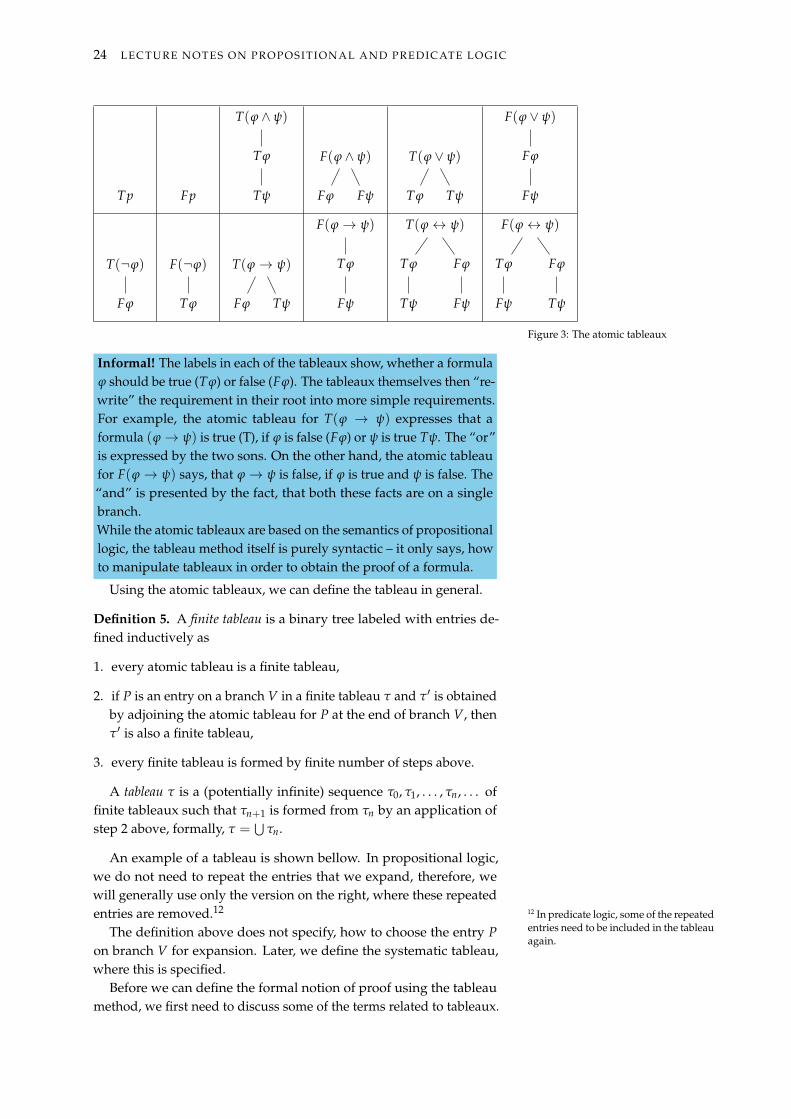
We already mentioned, that every tableau is a labeled binary tree.The nodes in the tree are labeled by entries, which are formulas with asign T/F that represent the assumption the formula is true (T) or false(F). The tree will be constructed using the atomic tableaux and a set ofrules. For a propositional variable p and propositions φ, ψ, the atomictableaux are given in the figure bellow.
24 LECTURE NOTES ON PROPOSITIONAL AND PREDICATE LOGIC
Tp Fp
T(φ ∧ ψ)
Tφ
Tψ
F(φ ∧ ψ)
Fφ Fψ
T(φ ∨ ψ)
Tφ Tψ
F(φ ∨ ψ)
Fφ
Fψ
T(¬φ)
Fφ
F(¬φ)
Tφ
T(φ→ ψ)
Fφ Tψ
F(φ→ ψ)
Tφ
Fψ
T(φ↔ ψ)
Tφ
Tψ
Fφ
Fψ
F(φ↔ ψ)
Tφ
Fψ
Fφ
Tψ
Figure 3: The atomic tableaux
Informal! The labels in each of the tableaux show, whether a formulaφ should be true (Tφ) or false (Fφ). The tableaux themselves then “re-write” the requirement in their root into more simple requirements.For example, the atomic tableau for T(φ → ψ) expresses that aformula (φ→ ψ) is true (T), if φ is false (Fφ) or ψ is true Tψ. The “or”is expressed by the two sons. On the other hand, the atomic tableaufor F(φ→ ψ) says, that φ→ ψ is false, if φ is true and ψ is false. The“and” is presented by the fact, that both these facts are on a singlebranch.While the atomic tableaux are based on the semantics of propositionallogic, the tableau method itself is purely syntactic – it only says, howto manipulate tableaux in order to obtain the proof of a formula.
Using the atomic tableaux, we can define the tableau in general.
Definition 5. A finite tableau is a binary tree labeled with entries de-fined inductively as
1. every atomic tableau is a finite tableau,
2. if P is an entry on a branch V in a finite tableau τ and τ′ is obtainedby adjoining the atomic tableau for P at the end of branch V, thenτ′ is also a finite tableau,
3. every finite tableau is formed by finite number of steps above.
A tableau τ is a (potentially infinite) sequence τ0, τ1, . . . , τn, . . . offinite tableaux such that τn+1 is formed from τn by an application ofstep 2 above, formally, τ =
⋃τn.
An example of a tableau is shown bellow. In propositional logic,we do not need to repeat the entries that we expand, therefore, wewill generally use only the version on the right, where these repeatedentries are removed.12 12 In predicate logic, some of the repeated
entries need to be included in the tableauagain.
The definition above does not specify, how to choose the entry Pon branch V for expansion. Later, we define the systematic tableau,where this is specified.
Before we can define the formal notion of proof using the tableaumethod, we first need to discuss some of the terms related to tableaux.

FORMAL PROOF SYSTEMS 25
F(((p→ q)→ p)→ p)
T((p→ q)→ p)
Fp
T((p→ q)→ p)
F(p→ q)
F(p→ q)
Tp
Fq
⊗
Tp
⊗
F(((p→ q)→ p)→ p)
T((p→ q)→ p)
Fp
F(p→ q)
Tp
Fq
⊗
Tp
⊗
Figure 4: Example tableau. The rectan-gles on the left show the atomic tableauxused. The version on the right removesthe repeated entries. The symbol ⊗ de-notes a contradictory branch.
For an entry P on a branch V in a tableau τ, we say that P is reducedon V if it occurs on V as a root of an atomic tableau. A branch V iscontradictory if it contains entries Tφ and Fφ for some propositionφ, otherwise it is noncontradictory. A branch V is finished, if it iscontradictory, or every entry on V is reduced on V, and finally, a tableauτ is finished if every branch in τ is finished and τ is contradictory, ifevery branch in τ is contradictory.
A tableau proof of φ is a contradictory tableau with the root entryFφ. A formula φ is tableau provable (⊢ φ) if it has tableau proof. On theother hand, a refutation of φ by tableau is a contradictory tableau withthe root entry Tφ, and φ is tableau refutable it it has a tableau refutation,in this case we write ⊢ ¬φ.
Informal! Why does a tableau proof of φ start with Fφ? Tableauxin fact represent systematic searches for assignments that fulfill thecondition expressed by the entry in the root. Therefore, if we cannotfind a truth assignment in which φ is false (the tableau for Fφ iscontradictory), then φ must be true in all assignments, and thereforevalid. The formal proof of the soundness and completeness of thetableau methods will be discussed shortly.
Figure 5 shows a tableau with the root entry F(((¬p ∧ ¬q) ∨ p)→(¬p ∧ ¬q)). The tableau has three branches, the leftmost one is con-tradictory, as it contains both F(¬p ∧ ¬q) and T(¬p ∧ ¬q), the middleone is finished and noncontradictory, as every entry on that branchis expanded on it, and the rightmost one is unfinished, as the entryF(¬q) is not expanded on that branch.
On the other hand, the tableau in Figure 4 is a tableau proof ofthe proposition (((p → q) → p) → p), as it starts with the entryF(((p→ q)→ p)→ p) and all its branches are contradictory.

26 LECTURE NOTES ON PROPOSITIONAL AND PREDICATE LOGIC
F(((¬p ∧ ¬q) ∨ p)→ (¬p ∧ ¬q))
T((¬p ∧ ¬q) ∨ p)
F(¬p ∧ ¬q)
T(¬p ∧ ¬q)
⊗
Tp
F(¬p)
Tp
F(¬q)
Figure 5: Example tableau. Both left andmiddle branches are finished. The leftone is also contradictory, while the mid-dle one is noncontradictory. The rightbranch is not finished.
We often need to work with theories, and also prove propositionsin a theory. Therefore, the notion of tableau needs to be generalized tothe notion of tableau from a theory. Theories provide axioms, theseare assumed to be true, and therefore the tableau from a theory T canadditionally contain entries of the from Tφ for an axiom φ ∈ T. Moreformally, a finite tableau from a theory T is a generalized tableau with anadditional rule – if V is a branch of finite tableau (from T) and φ ∈ T,then by adjoining Tφ at the end of V we obtain a finite tableau fromT. The rest of the definitions related to tableaux can be generalized inthe same way. A tableau from T is a sequence τ0, τ1, . . . , τn, . . . of finitetableaux from T such that τn+1 is formed from τn applying the rule 2(from the definition of tableaux), or the additional rule above, formallyτ =
⋃τn. A tableau proof of φ from T is a contradictory tableau from
T with Fφ in the root. T ⊢ φ denotes that φ is tableau provable fromT. A refutation of φ by a tableau from T is a contradictory tableau fromT with Tφ in the root. A branch V of a tableau from T is finished, ifit is contradictory, or every entry on V is already reduced on V and,additionally, V contains Tφ for each φ ∈ T.
While the current definition of tableaux is enough for proving propo-sitions in theories, here we provide a stricter definition of so calledsystematic tableau. We will see later, that a systematic tableau is al-ways finished and, in case the tableau is a proof of a proposition, it isalso finite. The definition prescribes the precise order of steps to usewhile constructing tableaux from theories – it specifies which entry inthe tableau should be expanded next and also which axiom from thetheory should be added next.
Definition 6. Let R be an entry and T = {φ0, φ1, . . . } a theory. Thenthe systematic tableau τ from T for the entry R is the result of thefollowing construction, i.e. τ =
⋃τn
1. t0 is the atomic tableau for R, then proceed with the following stepsuntil possible
2. Let P be the leftmost entry in the smallest possible level of thetableau τn, such that P is not reduced on some noncontradictorybranch through P.
FORMAL PROOF SYSTEMS 27
3. Let τ′n be the tableau obtained from τn by adjoining the atomictableau for P to every noncontradictory branch through P (τ′n = τn
if no such P exists).
4. Let τn+1 be the tableau obtained from τ′n by adjoining Tφn to everynoncontradictory branch that does not contain Tφn (if φn does notexist, τn+1 = τ′n).
The first thing to notice is that every systematic tableau is finished.Assume we have a tableau τ =
⋃τn. If there is a noncontradictory
branch in τ, the prefix of this branch is noncontradictory in each τn.Therefore, the branch must contain Tφn for each φn in T. Let us nowassume, there is an entry R, such that R is not reduced on a branch.However, there are only finitely many levels above R in τ and thereforeonly finitely many entries above R, thus R will be eventually selectedin step 2 and reduced in step 3, which is a contradiction with R notbeing reduced. So, every noncontradictory branch in the tableau isfinished (it contains Tφn for each φn ∈ T, and every entry on thebranch is reduced).
Interestingly, if tableau is used as a proof, it is not only finished, it isalso finite. More specifically – for every contradictory tableau τ =
⋃tn,
there is some n such that τn is contradictory finite tableau. Why? Let Sbe the set of nodes in τ that have no pair of contradictory entries Tφ,Fφ amongst their predecessors. We can imagine this set as a “top part”of the tableau – the root is definitely in this set. If there is a node in theset, all of its predecessors are also there. Such a set S must be finite,because otherwise, by König’s lemma, the subtree of τ induced by theset S would have an infinite branch (it is a finitely branching infinitetree), and therefore the tableau τ would not be contradictory. Now,since S is finite, all of the nodes in S belong to levels up to m for somem. Thus every node in level m + 1 has a pair of contradictory entriesamong its predecessors. We can now choose n such that the top m + 1levels of τ are a subtree of τn. Every branch in τn now contains a pairof contradictory entries and is thus contradictory.
In the construction of systematic tableaux, we extend only noncon-tradictory branches, therefore if a systematic tableau (from a theory) isa proof, it is finite (remember that a proof is a contradictory tableauwith Fφ in its root). This is an important results, it shows that if aformula has a proof, we have an algorithm (the construction of sys-tematic tableau) that can find the proof in finite amount of time. It alsoshows that any proof from a theory depends only on a finite numberof axioms from the theory.
Soundness and Completeness
Now, we want to show the soundness and completeness of the tableaumethod. We start with the soundness and show, that if a formulahas a tableau proof from a theory, the formula is also valid in thetheory. However, before we get to the proof, we need a definition anda lemma. We say that an entry P agrees with an assignment v, if P is Tφ

28 LECTURE NOTES ON PROPOSITIONAL AND PREDICATE LOGIC
and v(φ) = 1, or if P is Fφ and v(φ) = 0. A branch V agrees with v ifevery entry on V agrees with v.
Lemma 2. Let v be a model of a theory T that agrees with the root entry of atableau τ =
⋃τn. Then τ contains a branch that agrees with v.
Proof. We will find a sequence V0, V1, . . . for every n, such that Vn is abranch in τn, Vn ⊆ Vn+1 and Vn agrees with n. We start by verifying thelemma for all atomic tableaux, thus verifying the base of the induction.For example, if we have v(p) = 1, v(q) = 0 and the atomic tableauwith root entry T(p ∨ q), then v agrees with the root entry, and thebranch of the tableau containing Tp also agrees with v. We can checkthe other atomic tableaux similarly. Now, if τn+1 is obtained from τn
without extending Vn, we take Vn+1 = Vn. If τn+1 is obtained fromτn by adjoining Tφ to Vn for some φ ∈ T, let Vn+1 be this branch, vagrees with Vn+1 as v is a model of T (and therefore all axioms of Tare true in v). Finally, if τn+1 is obtained from τn by adjoining theatomic tableau for some entry P on Vn to the end of Vn, we can extendVn to Vn+1 as required as P agrees with v and all atomic tableaux areverified (for example, if P = T(p∨ q), and v is as in example on atomictableaux above, we obtain Vn+1 by adding T(p ∨ q) and Tp to the endof Vn).
Using the lemma, we can now easily proof the soundness of thetableau method in propositional logic.
Theorem 4 (Soundness of tableau method in propositional logic). Forevery theory T and proposition φ, if φ is tableau provable from T, then φ isvalid in T, i.e. T ⊢ φ⇒ T ⊨ φ.
Proof. If the proposition φ is tableau provable from T, there is a con-tradictory tableau τ from T with the root entry Fφ. Suppose φ is notvalid in T. In such a case, there is a model v of the theory T in whichφ is false. Therefore, the root entry of the proof (Fφ) agrees with vand by the previous lemma, there is a branch in τ that agrees withv. However, that leads to contradiction as τ is the proof of φ from T,and therefore every branch of τ is contradictory and cannot agree withv.
The soundness theorem says that whenever we have a tableau proofof a formula in a theory, the formula is valid. However, can we alsoprove any valid formula using the tableau method? We indeed can,as the completeness theorem states. Again, before we get to the proofof the completeness theorem, we prove a helper lemma, that formallyshows that a noncontradictory branch in a finished tableau provides acounterexample.
Lemma 3. Let V be a noncontradictory branch of a finished tableau τ. ThenV agrees with the following assignment v:
v(p) =
{1 if Tp occurs on V0 otherwise

FORMAL PROOF SYSTEMS 29
Proof. We prove the lemma by induction on the structure of formulasin entries on V.
• For entry Tp on V, where p is a propositional variable, we havev(p) = 1 by definition.
• For entry Fp on V, the entry Tp is not on V as V is noncontradictory,and thus we have v(p) = 0 by definition.
• For entry T(φ ∧ ψ), we have both Tφ and Tψ on V as τ is finished,and by induction, we know v(φ) = v(ψ) = 1, therefore v(φ ∧ ψ) =
1 and v agrees with T(φ ∧ ψ).
• For entry F(φ∧ψ), we have Fφ or Fψ on V as τ is finished, thereforewe have v(φ) = 0, or v(ψ) = 0, which leads to v(φ ∧ ψ) = 0 andthus v agrees with F(φ ∧ ψ).
The lemma can be proven for the other possible types of entries(with ∨,→,↔,¬) similarly to the last two steps for entries with ∧.
Using this lemma, it is simple to prove the completeness theorem.
Theorem 5. For every theory T and proposition φ, if φ is valid in T, then φ
is tableau provable from T, i.e. T ⊨ φ⇒ T ⊢ φ.
Proof. We will show that an arbitrary finished tableau τ from theoryT with root entry Fφ is contradictory, if φ is valid in T.
Assume (for contradiction), there is a noncontradictory branch Vin τ. The previous lemma provides an assignment v, such that Vagrees with v, therefore also the root entry Fφ agrees with v and thusv(φ) = 0. Since V is finished, it contains Tψ for every ψ ∈ T, but thatmeans that v is a model of T (V agrees with v, therefore v(ψ) = 1 forall ψ ∈ T). However, this is contradiction with the assumption thatφ is valid in T, therefore every branch in τ is contradictory and τ is aproof of φ from T.
We can now introduce syntactic definition of the semantic termsdefined earlier and discuss the relation between the syntactic andsemantic notions. First of all, we define the set of propositions provablefrom T
ThmP(T) = {φ|φ ∈ VFP, T ⊢ φ} .
We say that a theory T is inconsistent, if T ⊢ ⊥, otherwise T is consistent.A theory T is complete, if it is consistent and every proposition isprovable or refutable from T, i.e. if T ⊢ ¬φ or T ⊢ φ for everyφ ∈ VFP. A theory T over P is an extension of T′ over P′, if P′ ⊆ P
and ThmP′(T′) ⊆ ThmP(T), the extension is simple, if P = P′, and itis conservative if ThmP′(T′) = ThmP(T) ∩VFP′ . Two theories T and T′
are equivalent, if T is an extension of T′ and vice versa.There are strong relations between the syntactic terms introduced
above and the semantic terms introduced in the previous chapter. Mostof these are corollaries of the soundness and completeness of tableaumethod. For each theory T and propositions φ, ψ over P

30 LECTURE NOTES ON PROPOSITIONAL AND PREDICATE LOGIC
1. T ⊢ φ if and only if T ⊨ φ ,
2. ThmP(T) = θP(T) ,
3. T is inconsistent if and only if T is unsatisfiable, i.e. it has no model,
4. T is complete if and only if T is semantically complete, i.e. it has asingle model,
5. (deduction theorem) T ∪ {φ} ⊢ ψ if and only if T ⊢ φ→ ψ .
Another important corollary of the theorems is the compactnesstheorem.
Theorem 6. A theory T has a model if and only if every finite subset of Thas a model.
Proof. The implication to the right (if a theory has a model, every finitesubset has a model) is trivial. In order to prove the other implication,we first realize that if T has no model, it is inconsistent, thus T ⊢ ⊥ and⊥ is provable by a systematic tableau τ from T. The tableau is finite,therefore τ is also provable from a finite subset of T′ ⊆ T (T′ containsthe axioms from T that were used in the proof), T′ is inconsistent and,therefore, has no model.
While the compactness theorem is interesting itself, it is also avery strong theorem that can be used to prove other theorems indifferent parts of mathematics. Consider for example the theorem oninfinite k-colorable graphs13: a countably infinite graph G = (V, E) is 13 A graph is k-colorable if there is a func-
tion c : V → k, such that c(u) = c(v) forevery edge {u, v} ∈ E.
k-colorable if and only if each finite subgraph of G is k-colorable. Again,if the infinite graph is colorable, every finite subgraph is obviously alsocolorable. The other implication is more interesting. Consider a set ofpropositional variables P = {pu,i|u ∈ V, i ∈ k}, where pu,i means thatvertex u has color i. We can create a theory T with axioms pu,0 ∨ pu,1 ∨· · · ∨ pu,k−1 for each u ∈ V (every vertex has a color), ¬(pu,i ∧ pu,j)
for every u ∈ V, i < j < k (every vertex has only one color), and¬(pu,i ∧ pv,i) for each {u, v} ∈ E, i < k (two vertices connected withan edge do not have the same color). Obviously, G is colorable if andonly if T has a model. We only need to show, that every finite T′ ⊆ Thas a model (and use the compactness theorem). Let G′ be a subgraphof G induced by vertices u such that pu,i appears in T′ for some i. Byassumption, G′ is k-colorable, and therefore T′ has a model.
Hilbert systems
A (more traditional) alternative to the tableau method is the Hilbertcalculus. In this proof system, formulas are defined using only implica-tion (→) and negation (¬), and all other logical connectives are definedusing these two (we already know, that the set {→,¬} is adequate, sothis can be done). The Hilbert proof system then defines the followingset of schemas of axioms (for two proposition φ, ψ ∈ VFP):
1. φ→ (ψ→ φ)

FORMAL PROOF SYSTEMS 31
2. (φ→ (ψ→ χ))→ ((φ→ ψ)→ (φ→ χ))
3. (¬φ→ ¬ψ)→ (ψ→ φ)
Apart from the axioms, there is also a single inference rule: modusponens, which can be expressed as
φ, φ→ ψ
ψ.
That means that if φ and φ → ψ are true we can infer that also ψ istrue.
A proof of formula φ from a theory T in the Hilbert-style is definedas a finite sequence of formulas φ0, φ1, . . . φn = φ such that for everyi ≤ n, φi is a logical axiom, or an axiom from the theory (φn ∈ T), orφi is inferred from φj and φk (j, k < i) using the modus ponens rule.As with tableau method, a formula φ is provable from T (T ⊢H φ), if ithas a proof.
For example, we can show, that φ→ ψ is provable from T = {¬φ}for every ψ.
1. ¬φ
2. ¬φ→ (¬ψ→ ¬φ)
3. ¬ψ→ ¬φ
4. (¬ψ→ ¬φ)→ (φ→ ψ)
5. φ→ ψ
The first two steps are axiom of a theory and logical axiom (theschema number 2). The third formula is obtained from the previoustwo by modus ponens, the fourth one is again an axiom (by schemanumber 3), and the last one is obtained from formulas number 3 and 4using modus ponens.
It is easy to prove the soundness of the Hilbert calculus (T ⊢H φ⇒T ⊨ φ). Logical axioms are tautologies, and axioms from T hold in allmodels of T, therefore the soundness holds for axioms of any kind,and the modus ponens rule is sound (as can be easily checked usingthe truth tables of φ, φ → ψ, and ψ). Thus, the soundness is proved.The Hilbert calculus is also complete, but we will not show the proofhere.
Resolution method
The resolution method is the base of many automated systems – SATsolvers, automated deduction or verification systems and Prolog14 14 Prolog is a programming language
based on the specification of programsas sets of Horn formulas.
interpreters. The method assumes the input formulas are given inCNF and it works with a set representation of the formulas (a CNFformula is represented as a set of sets of literals). The method has noexplicit axioms, but some of the axioms are implicitly included. It usesa single inferences rule (the resolution rule). Similarly to the tableau

32 LECTURE NOTES ON PROPOSITIONAL AND PREDICATE LOGIC
method, the resolution method is also a refutation procedure, i.e. ittries to show that a given formula or theory is unsatisfiable. There areseveral variants of the resolution method that gives more specific ruleson when the resolution rule can be applied (e.g. the LI resolution, orthe SLD resolution).
Before we describe the resolution method formally, we must definethe set representation of CNF formulas. Similarly to our discussion onCNF formulas, a literal is either a propositional variable or its negation.The complementary literal to l is still denoted as l. A clause C is a finiteset of literals, and an empty clause, denoted as □ , is never satisfied. Aformula S is then a (possibly infinite) set of clauses. An empty formula∅ is always satisfied. Infinite formulas represent infinite theories. A(partial) assignment V is a consistent set of literals (i.e. the set does notcontain a complementary pair of literals). An assignment is total, if itcontains a positive or negative literal for each propositional variable.An assignment V satisfies a formula S (denoted as V ⊨ S), if C∩V = ∅for each clause C ∈ S.
For example, the CNF-formula ((¬p ∨ q) ∧ (¬p ∨ ¬q ∨ r) ∧ (¬r ∨¬s) ∧ s) is represented as S = {{¬p, q}, {¬p,¬q, r}, {¬r,¬s}, {s}}and V = {s,¬r,¬p} is a satisfying assignment for S.
Informal! While the definitions above are different from those weused previously, they are in fact equivalent. The only reason whythey are worded differently is the set representation of the CNFformulas. We know that a formula in CNF is a conjunction of clauses,therefore, we can only represent them as a set of clauses. A clause isa disjunction of literals, and therefore it is again natural to representeach clause as a set of literals. The definition of assignment may seemstrange, but the set of literals only says which literals are true andwhich are false.
There is only one inference rule in resolution – the resolution rule:let C1 and C2 are clauses such that l ∈ C1 and l ∈ C2, then infer aclause C (called a resolvent) such that C = (C1 \ {l}) ∪ (C2 \ {l}). Theresolution rule is a special case of the cut rule:
φ ∨ ψ ¬φ ∨ χ
ψ ∨ χ,
for any formulas φ, ψ, χ.It is easy to realize that the resolution rule is sound, i.e. if V ⊨ C1
and V ⊨ C2, then V ⊨ C – the assignment V cannot contain a pairof complementary literals (by definition), therefore at least one ofthe intersections V ∩ (C1 \ {l}) or V ∩ (C2 \ {l}) must be non-empty,therefore V ∩ C is also non-empty.
A resolution proof (deduction) of a clause C from formula S is a finitesequence of clauses C0, C1, . . . , Cn = C such that for each i ≤ n, Ci ∈ S,or Ci is a resolvent of some previous clauses. As usual, a clause C isprovable from formula S (S ⊢R C), if it has a resolution proof from S. Wealready mentioned that resolution is used as a refutation procedure.A resolution refutation of formula S is a resolution proof S ⊢R □, and aformula is resolution refutable, if there is such a proof.
FORMAL PROOF SYSTEMS 33
Let us now show, that resolution is also a sound and completemethod. The soundness is simple, and follows from the soundness ofthe resolution rule.
Theorem 7 (Soundness of resolution). If a formula S is resolution refutable,it is unsatisfiable.
Proof. Let S ⊢R □ and assume (for contradiction) there is an assign-ment V such that V ⊨ S. Because the resolution rule is sound, alsoV ⊨ □, but that is not possible (□ is never satisfied).
The proof of completeness is a bit more involved. To this end, wefirst define resolution trees, which in fact show, how we obtained aproof of a clause. A resolution tree of clause C from formula S is a finitebinary tree with nodes labeled by clauses such that the root is labeledby C, the leaves are labeled by clauses from S, and every inner nodeis labeled by the resolvent of its sons. Obviously, there is a resolutiontree for C from S if and only if S ⊢R C.
Another important notion is the resolution closure of a formula S,denoted asR(S) and defined as the smallest set containing all clausesof S and closed under the resolution rule, i.e. if C1, C2 ∈ R(S) and C isthe resolvent of C1 and C2, then also C ∈ R(S). Obviously, C ∈ R(S)if and only if S ⊢R C, and all the notions on resolution proofs can bealso defined using the resolution trees and closures.
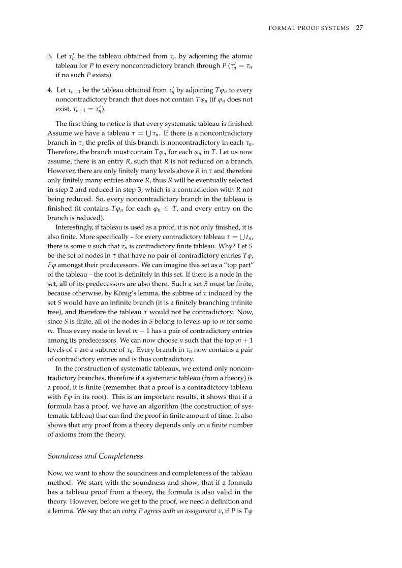
As a simple example of the resolution method, we can show that for-mula S = {{p, r}, {q,¬r}, {¬q}, {¬p, t}, {¬s}, {s,¬t}} is unsatisfiableas S ⊢R □.
□
{p}
{p, q}
{p, r} {q,¬r}
{¬q}
{¬p}
{¬p, s}
{¬p, t} {s,¬t}
{¬s}
Figure 6: The resolution proof of S ⊢R □.
We can also compute the resolution closure
R(S) = {{p, r}, {q,¬r}, {¬q}, {¬p, t}, {¬s}, {s,¬t}, {p, q},{¬r}, {r, t}, {q, t}, {¬t}, {¬p, s}, {r, s}, {t}, {q},{q, s},□, {¬p}, {p}, {r}, {s}} ,
and as □ ∈ R(S), we also know that S in unsatisfiable.In the proof of completeness, we will use the notion of reduction by
substitution. Let S be a formula and l a literal, we define
Sl = {C \ {l}|l /∈ C ∈ S} .
The new formula Sl is in fact equivalent to a formula, where the literall was assigned a true value (⊤) and l was assigned false value (⊥). In

34 LECTURE NOTES ON PROPOSITIONAL AND PREDICATE LOGIC
such a case, any clause containing l can be removed (as it is satisfied),and l is removed from all other clauses. The formula Sl does notcontain any of the literals l and l, and if S contained a clause {l}, thenSl contains □.
In the proof of completeness of the resolution method, we will needthe following lemma.
Lemma 4. A formula S is satisfiable if and only if Sl or Sl is satisfiable.
Proof. Let V ⊨ S and (without loss of generality) l ∈ V . Then, V ⊨ Sl ,as for clauses C such that l /∈ C ∈ S, V ⊨ C \ {l}, as V does not contain{l} and it is satisfying for each clause C ∈ S.
On the other hand, assume (without loss of generality) V ⊨ Sl forsome V . Since neither l nor l occur in Sl , V ′ = (V \ {l) ∪ {l}} ⊨ Sl .Then, V ′ ⊨ S, as for C ∈ S, such that l ∈ C, also l ∈ V and for C ∈ Snot containing l, we have V ′ ⊨ (C \ {l}) ∈ Sl .
The reductions of literals can be represented in a binary tree – socalled reduction tree. The root of the tree is the formula S and eachnode N has two sons – Nl and N l . With the reduction tree, formula Sis unsatisfiable if and only if every branch contains □.
S = {{p}, {¬q}, {¬p,¬q}}
Sp = {{¬q}}
Spq = {□} Spq = ∅
S p = {□, {¬q}}
Figure 7: An example of a reduction tree.
Interestingly, since S can be infinite over countable language, thetree can also be infinite. However, if S is unsatisfiable, accordingto the compactness theorem, there is a finite S′ ⊆ S such that S′ isunsatisfiable. Therefore, after the reduction of all literals from S′, therewill be □ on every branch after finitely many steps.
Finally, we can prove the completeness of the resolution. The the-orem bellow shows the completeness for finite formulas, the generalversion is obtained from that theorem by using the compactness, simi-larly to the discussion on the reduction trees above.
Theorem 8 (completeness of resolution). If a finite S is unsatisfiable, it isresolution refutable, i.e. S ⊢R □.
Proof. We will prove the theorem by induction on the number ofvariables in S. There is only one unsatisfiable S without variables – {□}and therefore S ⊢R □ (the proof is the single step □).
Let us now assume, that S is unsatisfiable and contains a literal l.Then, by the previous lemma, Sl and Sl are unsatisfiable. These containless literals than S and therefore by induction there are resolution treesTl and T l for derivation of □ from Sl and Sl respectively. Now, if everyleaf of Tl is in S, then Tl is a resolution tree of □ from S and thereforeS ⊢R □. Otherwise, we can append the literal l to each leaf of Tl whichis not in S and to all of its predecessors, thus obtaining the resolution

FORMAL PROOF SYSTEMS 35
tree for {l} from S (if the original leaf was not in S, the one with addedl will be, as the only difference between Sl and S is the removal of l).Similarly, by appending {l} to leaves in T l we obtain resolution treefor {l} from S. Resolving the roots of these trees yields the resolutiontree of □ from S.
We already mentioned that resolution is widely used in differentautomated systems – SAT solvers, formal verification systems etc.One of the important examples is the Prolog interpreter. Prolog is aprogramming language, where programs are sets of Horn clauses. Theprogram can then answer queries (goals). As the Prolog programs arelimited to Horn formulas, the resolution method can be improved. TheProlog interpreter uses so called SLD resolution which is based on LDresolution and that is in turn based on LI resolution, which is a specialcase of linear resolution. Therefore, we will now define the linearresolution, show that LI resolution is complete for Horn formulas andfinally define the LD and SLD resolution as simple improvements ofthe LI resolution.
Linear resolution
The general resolution procedure can be further simplified withoutlosing the completeness. We define a linear proof of a clause C from aformula S as a finite sequence of pairs (C0, B0), . . . , (Cn, Bn), such thatC0 ∈ S and for every i ≤ n, Bi ∈ S or Bi = Cj for some j < i, and Ci+1
is a resolvent of Ci and Bi, where Cn+1 = C. In the linear proof C0 iscalled the starting clause, Ci a central clause, and Bi a side clause. Again,we say that C is linearly provable from S (S ⊢L C), if it has a linear prooffrom S. A linear proof of □ from S is a linear refutation of S and S islinearly refutable if S ⊢ □.
Obviously, every linear proof can be transformed into a general reso-lution proof and therefore the linear resolution is also sound. Moreover,is is also complete (we omit the proof of completeness here).
LI-resolution
If we deal with Horn formulas, we can use an even more refinedresolution procedure called linear input (LI) resolution. A LI-resolutionfrom a formula S is a linear resolution from S where each side clauseBi is from the input formula S (i.e. Bi cannot be a previously resolvedcentral clause). We write S ⊢LI C to denote that C is provable byLI-resolution from S.
We already defined Horn formulas while discussing the satisfiabilityproblem. The definition from the resolution point of view is similar,the only difference is that we again use the set representation insteadof the general one (and also formulas in this case can be infinite, asthere is no distinction between theories and formulas in resolution).So, a Horn clause is a finite set of literals containing at most one positiveliteral. A Horn formula is then a (potentially infinite) set of Hornclauses. A clause {p}, where p is a positive literal is called a fact, and a

36 LECTURE NOTES ON PROPOSITIONAL AND PREDICATE LOGIC
clause with exactly one positive literal is called a rule. Rules and factsare also called program clauses. A non-empty Horn clause without anypositive literal is called a goal.
We can easily see that if a Horn formula S is unsatisfiable and it doesnot contain □, it must contain some fact and some goal. Why? If Sdoes not contain any fact, it is satisfied by setting all the propositionalvariables to 0. if it does not contain any goal, it is satisfied by settingall variables to 1.
The LI-resolution is complete for Horn formulas, as the followingtheorem says. The proof of the theorem is similar to the proof ofcompleteness of general resolution.
Theorem 9 (completeness of LI-resolution). If T is satisfiable Horn for-mula but T ∪ {G} is unsatisfiable for some goal G, then □ a LI-resolutionfrom T ∪ {G} with starting clause G.
Proof. As in the proof of completeness of general resolution, we useinduction on the number of variables, this time in T. By the observationabove, T must contain a fact {p} for some variable p (T ∪ {G}) isunsatisfiable, therefore it must contain a goal and a fact, G is a goal,so the fact must be in T). By the lemma we used in the proof ofcompleteness of general resolution, T′ = (T ∪ {G})p = Tp ∪ {Gp} isunsatisfiable and Gp = G \ {¬p}. Now, if Gp = □, we have G = {¬p}and thus □ is a resolvent of G and {p} ∈ T. Otherwise, since Tp issatisfiable (by the satisfying assignment for T) and has less variables,by induction assumption, there is an LI-resolution of □ form T′ startingwith Gp. If we now append the literal ¬p to all leaves that are notin T ∪ {G} (and their predecessors), we have an LI-resolution proofof {¬p} from T, we can resolve it with {p} from T to obtain the LI-resolution proof of □ from T.
Resolution in Prolog
A program in Prolog is a set of program clauses (i.e. rules or facts),an example program is shown bellow (the program contains sevenclauses, the numbers indicate line numbers and are not a part of theprogram):
1: p:-q,r. 5: r.
2: p:-s. 6: s:-t.
3: q. 7: s.
4: q:-s.
The formulas on lines 3, 5, and 7 are facts, the rest are rules. Thesymbol :- can be interpreted as an implication from right to left (←).So, the meaning of the clauses is as given bellow:
1. q ∧ r → p
2. s→ p
3. q
4. s→ q

FORMAL PROOF SYSTEMS 37
5. r
6. t→ s
7. s
In Prolog, we want to know whether a query is a consequence ofa given program. A query is a conjuction of goals (positive literals),e.g. p ∧ q. That means, the question is, whether for a program Pand query (q1 ∧ · · · ∧ qn), it holds that P ⊨ (q1 ∧ · · · ∧ qn). However,such a question is equivalent to the fact that P ∪ {¬q1, . . . ,¬qn} isunsatisfiable, which is equivalent to □ having LI-resolution from P ∪{G} starting with goal G = {¬q1, . . . ,¬qn}.
In the Prolog interpreter, the clauses are represented as sequencesof literals (as opposed to sets of literals as in LI resolution). Therefore,Prolog uses a slightly different version of LI-resolution called the LD-resolution (linear definite). In LD resolution, the resolvent of a goal(¬p1, . . . ,¬pi−1,¬pi,¬pi+1, . . . ,¬pn) and a rule (pi,¬q1, . . . ,¬qm) isa new goal (¬p1, . . . ,¬pi−1,¬q1, . . . ,¬qm,¬pi+1, . . . ,¬pn), i.e. one ofthe negative literals in the current goal is replaced by the negativeliterals from the rule.
The LD resolution does not specify, which of the negative literalsin the goal should be resolved next. This would make programmingin Prolog hard, therefore it extends the LD resolution with a selectionruleR. Typically, the rule is “select the first literal”. More formally, anSLD-resolution via R is an LD-resolution in which each step (Ci, Bi)
we resolve throughR(Ci).Obviously, any LI-resolution can be expressed as LD-resolution
(just use the sequences of literals instead of the sets of literals), andany LD-resolution can be expressed as an SLD-resolution with thecorrect selection rule (select the literal that was selected in the LDresolution). Therefore, we can see that SLD resolution is complete forProlog programs.
Further discussion on Prolog is out of the scope of this lecture, so wewill omit it here. The important message was to show an applicationof logic in computer science. Prolog is quite often used in certain areasof artificial intelligence.
This concludes the part of the lecture dedicated to propositionallogic. We started with the discussion about the syntax of propositions,explained their semantics and showed some formal proof systems. Inthe next part of the lecture, we will build on the understanding ofconcepts from propositional logic and extend them to predicate logic(more precisely to first order logic).


Part II
First-Order Logic


Basic Syntax and Semantics
We are now ready to discuss the predicate logic, mostly the first-orderlogic. The language of predicate logic is more expressive than the oneof propositional logic and allows us to express complex formulas in amuch more concise way. In propositional logic, we often needed to usemany variables and created long formulas. In predicate logic, someof these can be written more elegantly, as we can now use functions,relations, and logical quantifiers.
This whole part will follow the structure of the previous one – wewill again start by the basic syntax and semantics of predicate logic,then we will discuss the logical theories and their models, the tableaumethod in predicate logic and also the resolution method. While thebasic ideas remain the same, there are also important differences. Forexample, a model of a theory will now be defined as a mathematicalstructure in which all the axioms of the theory are true, instead of thesimpler definition as a truth assignment.
First-order formulas and theories
The symbols used in first-order language can be divided into twogroups – symbols of logic and non-logical symbols. The symbols of logicconsist of variables (x, y, z, . . . , x1, x2, · · · ∈ Var), logical connectives(→,∧,∨,↔,¬), the quantifiers (∀x), (∃x) for each variable x ∈ Var,and parenthesis.
The non-logical symbols consist of function symbols ( f , g, . . . ), includ-ing constant symbols (c, d, . . . ), which are nullary function symbols,and relation (predicate) symbols (P, Q, R). Each function and relationsymbol S, has an associated arity ar(S) ∈N that expresses the numberof arguments the symbol takes.
The equality (=) is a special relation symbol that is often consideredseparately, as it is central to many parts of mathematics and thereare even special axioms regarding the equality. Equality is also notconsidered a non-logical symbol.
The language in first-order logic is determined by the sets of func-tion and relation symbols – these are coupled in the so called signature,which is a pair ⟨R,F⟩ of relation and function symbols with their ari-ties. None of the symbols is the equality symbol. The language is thengiven by a signature L = ⟨R,F⟩ and by specifying whether the lan-guage is with equality or not. A language must always contain at leastone relation symbol (either equality or a non-logical one), otherwise, it
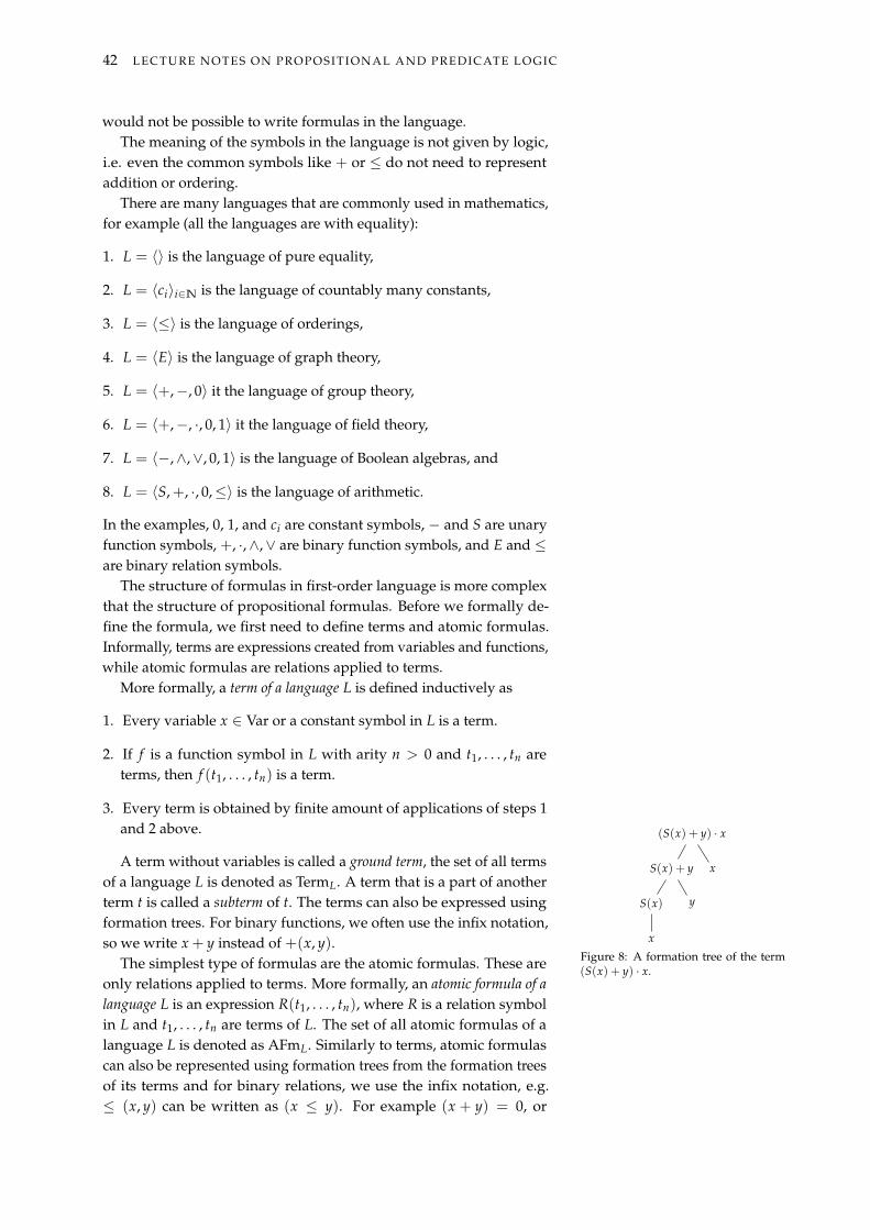
42 LECTURE NOTES ON PROPOSITIONAL AND PREDICATE LOGIC
would not be possible to write formulas in the language.The meaning of the symbols in the language is not given by logic,
i.e. even the common symbols like + or ≤ do not need to representaddition or ordering.
There are many languages that are commonly used in mathematics,for example (all the languages are with equality):
1. L = ⟨⟩ is the language of pure equality,
2. L = ⟨ci⟩i∈N is the language of countably many constants,
3. L = ⟨≤⟩ is the language of orderings,
4. L = ⟨E⟩ is the language of graph theory,
5. L = ⟨+,−, 0⟩ it the language of group theory,
6. L = ⟨+,−, ·, 0, 1⟩ it the language of field theory,
7. L = ⟨−,∧,∨, 0, 1⟩ is the language of Boolean algebras, and
8. L = ⟨S,+, ·, 0,≤⟩ is the language of arithmetic.
In the examples, 0, 1, and ci are constant symbols, − and S are unaryfunction symbols, +, ·,∧,∨ are binary function symbols, and E and ≤are binary relation symbols.
The structure of formulas in first-order language is more complexthat the structure of propositional formulas. Before we formally de-fine the formula, we first need to define terms and atomic formulas.Informally, terms are expressions created from variables and functions,while atomic formulas are relations applied to terms.
More formally, a term of a language L is defined inductively as
1. Every variable x ∈ Var or a constant symbol in L is a term.
2. If f is a function symbol in L with arity n > 0 and t1, . . . , tn areterms, then f (t1, . . . , tn) is a term.
3. Every term is obtained by finite amount of applications of steps 1and 2 above.
A term without variables is called a ground term, the set of all termsof a language L is denoted as TermL. A term that is a part of anotherterm t is called a subterm of t. The terms can also be expressed usingformation trees. For binary functions, we often use the infix notation,so we write x + y instead of +(x, y).
(S(x) + y) · x
S(x) + y
S(x)
x
y
x
Figure 8: A formation tree of the term(S(x) + y) · x.The simplest type of formulas are the atomic formulas. These are
only relations applied to terms. More formally, an atomic formula of alanguage L is an expression R(t1, . . . , tn), where R is a relation symbolin L and t1, . . . , tn are terms of L. The set of all atomic formulas of alanguage L is denoted as AFmL. Similarly to terms, atomic formulascan also be represented using formation trees from the formation treesof its terms and for binary relations, we use the infix notation, e.g.≤ (x, y) can be written as (x ≤ y). For example (x + y) = 0, or

BASIC SYNTAX AND SEMANTICS 43
R( f (x), g(y, z), x) are atomic formulas ( f is a unary function, g and +
are binary functions, and R is a ternary relation).We can finally define formulas in first-order language. The defini-
tion is similar to the one in propositional language, but this time thepropositional variables are represented by atomic formulas and weadditionally have the quantifiers. Formally, a formula of a language L isdefined inductively by
1. Every atomic formula is a formula
2. If φ and ψ are formulas, (φ→ ψ), (φ ∧ ψ), (φ ∨ ψ), (φ↔ ψ), (¬φ)
are also formulas.
3. If φ is a formula and x ∈ Var is a variable, then ((∀x)φ) and ((∃x)φ)
are formulas.
4. Every formula is obtained by a finite application of the steps above.
The set of all formulas of a language L is denoted by FmL. A formulathat is a part of another formula φ is a subformula of φ. Of course,formulas can also be expressed as their formation tree. An example ison the right.
(∀x)(x · y ≤ (S(x) + y) · x)
x · y ≤ (S(x) + y) · x
x · y
x y
(S(x) + y) · x
S(x) + y
S(x)
x
y
x
Figure 9: A formation tree of the formula(∀x)(x · y ≤ (S(x) + y) · x). Moreover,x · y and (S(x) + y) · x are roots of for-mation trees of the terms included in theformula.
As before, we can define some conventions to simplify writingthe formulas. After introducing priorities of binary function symbols(+, ·, . . . ) we can omit parenthesis in the infix notation of terms thatare around a subterm formed by a symbol of higher priority. We alsointroduce the priority of logical connectives similar to the prioritiesin the propositional logic. The negation and quantifiers (¬, (∀x), (∃x))have the highest priorities, then we have conjunction and disjunction(∧,∨) and, finally, the implication and equivalence (→,↔) have thelowest priority. Now, we can omit some of the parenthesis in theformulas.
In predicate logic, there is an important difference between so calledfree and bound (occurrences of) variables, as we deal with each typedifferently in the semantics. For a formula φ and variable x, an occur-rence of x in φ is a leaf labeled by x in the formation tree of φ. Theoccurrence of x in φ is bound, if it is in some subformula ψ that startswith (∀x) or (∃x). Otherwise the occurrence is free. A variable is freein a formula, if it has at least one free occurrence in the formula andit is bound if it has at least one bound occurrence. A variable can beboth free and bound at the same time. For example, in the formulax > 0∨ (∀x)(∃y)(x > y) the variable x is both free and bound, as itsfirst occurrence is free and the second one is bound. We will use thenotation φ(x1, . . . , xn) to denote that x1, . . . , xn are all the free variablesin φ.
A formula is open, if it contains no quantifiers. The set of allopen formulas in a language L will be denoted as OFmL. Obviously,AFmL ⊊ OFmL ⊊ FmL. On the other hand, a formula is closed (asentence) if it has no free variables. A formula can be both closed andopen at the same time, all terms of such formulas are ground terms.
In mathematics, we very often have general theorems and we lateruse them with a more specific substitutions. This can more formally be

44 LECTURE NOTES ON PROPOSITIONAL AND PREDICATE LOGIC
expressed by substituting terms for free variables in formulas, however,we need to be careful, as in some cases the substitution can change themeaning of the formula. For example, if we substituted the term y forx in (∃y)(x + y = 1), we would change the original meaning of theformula “there is a y such that y = 1− x” to a new meaning that says“y is divisible by 2”. We want to avoid such situation while performingthe substitution. Therefore, we define a term t is substitutable for avariable x in a formula φ, if after the substitution of t for all freeoccurrences of x, none of the variables of t become bound in φ. Thenew formula is denoted as φ(x/t) and we call it an instance of theformula φ after a substitution of term t for variable x. Alternatively,we can also define that t is not substitutable for x in φ if x has afree occurrence in a subformula of the form (∃y)ψ or (∀y)ψ for somevariable y in t.
We can also rename the quantified variables, but we again need tobe careful. In this case, we would like to obtain an equivalent formula.Let (Qx)ψ be a subformula of φ where Q is either ∀ or ∃ and y is avariable. Then, if y is substitutable for x in ψ and y is not free in ψ, wecan replace the subformula (Qx)ψ with (Qy)ψ(x/y) to obtain a variantof φ in subformula (Qx)ψ. A variant of φ is obtained by variation ofone or more subformulas of φ.
Informal! Creating variants in predicate logic serves some importantpurposes. One of them is, that we can easily transform any formulawith a variable that is both free and bound into its variant, whereeach variable is “pure”, i.e. only free or only bound. Moreover,we will very often create variants from formulas in order to fulfillassumptions such as “variable x is not free in φ”.
Semantics of first-order logic
In propositional logic, models were defined as truth assignments. Thetruth assignment was enough to tell whether a proposition is true orfalse. In predicate logic, the situation is a bit more complex. Firstof all, the values of variables can be taken from a larger set thanonly {0, 1}. Moreover, we need to define, what all the functions andrelations mean. A natural representation of models in first-order logicis a mathematical structure. A structure is a set and a definition offunctions and relations on this set.
More formally, if we have a signature of a language L = ⟨R,F⟩and a non-empty set A, a realization (interpretation) of a relation symbolR ∈ R on the set A is any relation RA ⊆ Aar(R). A realization of =is the identity relation on A, i.e. IdA = {(x, x)|x ∈ A}. A realization(interpretation) of a function symbol f ∈ F is any function f A : Aar( f ) →A. Specifically, a realization of a constant symbol is some element of A.A structure for the language L (L-structure) is a triple A = ⟨A,RA,FA⟩,where A is a non-empty set called the domain of the structure A,RA
is a collection of realizations of the relation symbols on A, and FA isa collection of realizations of function symbols on A. A structure of
BASIC SYNTAX AND SEMANTICS 45
the language is also called a model of the language, and the class of allmodels of a language L will be denoted as M(L).
You probably already know different mathematical structures fromother parts of mathematics, for example:
1. S = ⟨S,≤⟩ is an ordered set, where ≤ is reflexive, antisymmetric,and transitive binary relation,
2. G = ⟨V, E⟩ is a graph,
3. Zp = ⟨Zp,+,−, 0⟩ is the additive group of integers modulo p,
4. Q = ⟨Q,+,−, 0, 1⟩ is the field of rational numbers,
5. P(X) = ⟨P(X), \,∩,∪, ∅, X⟩ is the set algebra over X, and
6. N = ⟨N, S,+, ·, 0,≤⟩ is the standard model of arithmetic.
But also many other objects can be defined as structures, e.g. the finiteautomata or even databases.
We now aim to define the truth value of formulas in first-order logic.We already know, that a formula is constructed from atomic formulas,which are in turn constructed from terms. Therefore, in order to definethe truth value of a formula, we need to start with the definition of thevalue of a term. Let t be a term of L = ⟨R,F⟩ and A = ⟨A,RA,FA⟩an L-structure. A variable assignment over the domain A is a functione : Var→ A. The value tA[e] of the term t in the structureAwith respectto the assignment e is defined inductively by
1. xA[e] = e(x), for x ∈ Var,
2. ( f (t1, . . . , tn))A[e] = f A(tA1 [e], . . . , tA
n [e]) for f ∈ F .
For a constant symbol cA[e] = cA, i.e. the values of constants do notdepend on the assignment e, and therefore also the value of groundterms does not depend on the assignment. Obviously, the value of aterm t depends only on the assignment of variables in t.
We now know, how to compute the values of individual terms,therefore, we can define the value of atomic formulas. Contrary tothe values of terms, values of formulas are always from the set {0, 1}.Let φ be an atomic formula of L = ⟨R,F⟩ in the form R(t1, . . . , tn),A = ⟨A,RA,FA⟩ is an L-structure and e a variable assignment overA. The value HA
at(φ)[e] of the atomic formula φ in the structure A withrespect to e is
HAat(φ)[e] =
{1 if (tA
1 [e], . . . tAn [e]) ∈ RA
0 otherwise
Specifically, for the equality relation =, the only possible realizationis IdA and therefore HA
at(t1 = t2)[e] = 1, if tA1 [e] = tA
2 [e] and 0 other-wise. We can again see that the value of a formula depends only on theassignment of variables in the formula and that the value of a groundformula does not depend on the assignment at all.
We can finally define the value of a general formula. The definitionis quite long, but also very similar to the one in propositional logic. In

46 LECTURE NOTES ON PROPOSITIONAL AND PREDICATE LOGIC
fact, the only difference is in the last two cases. The atomic formulasin this case play the role of the propositional variables.
The value HA(φ)[e] of formula φ in the structure A with respect toe is
HA(φ)[e] = HAat(φ)[e] if φ is atomic
HA(¬φ)[e] = −1(HA(φ)[e])
HA(φ ∧ ψ)[e] = ∧1(HA(φ)[e], HA(ψ)[e])
HA(φ ∨ ψ)[e] = ∨1(HA(φ)[e], HA(ψ)[e])
HA(φ→ ψ)[e] =→1 (HA(φ)[e], HA(ψ)[e])
HA(φ↔ ψ)[e] =↔1 (HA(φ)[e], HA(ψ)[e])
HA((∀x)φ)[e] = mina∈A
(HA(φ)[e(x/a)])
HA((∃x)φ)[e] = maxa∈A
(HA(φ)[e(x/a)])
where −1,∧1,∨1,→1,↔1 are the functions given by the truth tables inthe part on propositional logic and e(x/a) is an assignment assigningvalue a to variable x and otherwise identical to e. We can see that thevalue of a formula depends only on the assignment of free variables inthe formula (we check all possible assignments for the bound variablesin steps 7 and 8).
The structure A satisfies the formula φ if HA(φ) = 1, we denotethe fact as A ⊨ φ[e], otherwise we write A ⊭ φ[e]. We can easily checkthat all the following hold
A ⊨ ¬φ[e]⇔ A ⊭ φ[e]
A ⊨ (φ ∧ ψ)[e]⇔ A ⊨ φ[e] and A ⊨ ψ[e]
A ⊨ (φ ∨ ψ)[e]⇔ A ⊨ φ[e] or A ⊨ ψ[e]
A ⊨ (φ→ ψ)[e]⇔ A ⊨ φ[e] implies A ⊨ ψ[e]
A ⊨ (φ↔ ψ)[e]⇔ A ⊨ φ[e] if and only if A ⊨ ψ[e]
A ⊨ (∀x)(φ)[e]⇔ A ⊨ φ[e(x/a)] for every a ∈ A
A ⊨ (∃x)(φ)[e]⇔ A ⊨ φ[e(x/a)] for some a ∈ A
Furthermore, if t is substitutable for x in φ, then for every structure Aand assignment e, A ⊨ φ(x/t)[e] if and only if A ⊨ φ[e(x/a)], wherea = tA[e]. If ψ is a variant of φ then A ⊨ φ[e] if and only if A ⊨ ψ[e].
As in propositional logic, we can generalize the notion above tovalidity in structure and in theory. Let φ be a formula of a language L,and A an L-structure. We say, that φ is valid in A, denoted as A ⊨ φ,if A ⊨ φ[e] for every e : Var → A. We also say that A satisfies φ.Otherwise, we write A ⊭ φ. The formula φ is contradictory in A ifA ⊨ ¬φ, i.e. if A ⊭ φ[e] for every e.
We can easily check, that for any structure A and formulas φ, ψ thefollowing holds:
A ⊨ φ⇒ A ⊭ ¬φ (1)
A ⊨ φ ∧ ψ⇔ A ⊨ φ and A ⊨ ψ (2)
A ⊨ φ ∨ ψ⇐ A ⊨ φ or A ⊨ ψ (3)
A ⊨ φ⇔ A ⊨ (∀x)φ (4)

BASIC SYNTAX AND SEMANTICS 47
Moreover, if φ and ψ are sentences, the implications in (1) and (3) arein fact equivalences. The last equivalence (4) also shows, that A ⊨ φ ifand only if A ⊨ ψ, where ψ is the universal closure of φ, i.e. the formula(∀x1)(∀x1) . . . (∀xn)φ, where x1, . . . , xn are all the free variables of φ.
A theory of a language L is any set T of formulas of L (the axioms ofthe theory). A model of a theory T is an L-structure A such that A ⊨ φ
for every φ ∈ T. We also write A ⊨ T and say that A satisfies T.The class of all models of theory T is M(T) = {A ∈ M(L)|A ⊨ T}. Aformula is valid in T (true in T) (T ⊨ φ) ifA ⊨ φ for every modelA of T.Otherwise we write T ⊭ φ. A formula φ is contradictory in T if T ⊨ ¬φ
and φ is independent in T if it is neither valid nor contradictory in T. Forempty theory T, we can omit T in the notation and M(T) = M(L). Inthis case, (⊨ φ) means that the formula φ is logically valid (a tautology).A consequence of T is the set θL(T) of all sentences of L valid in T, i.e.
θL(T) = {φ ∈ FmL |T ⊨ φ and φ is a sentence} .
Informal! The definitions above should closely resemble those wesaw in propositional logic, the main difference is in the definition ofthe model. In propositional logic, we could use truth assignments,while in predicate logic, the model is a structure. The structure, andits definitions of functions and relations in fact give the truth valuesto the atomic formulas. The atomic formulas then play the role of thepropositional variables. Of course, in predicate logic, we also need totake care of the quantifiers, which brings another complexity to thedefinitions.
For example, the theory of orderings T is a theory in languageL = ⟨≤⟩ with axioms
x ≤ x reflexivity,
x ≤ y ∧ y ≤ x → x = y antisymmetry,
x ≤ y ∧ y ≤ z→ x ≤ z transitivity.
The models of T (ordered sets) are structures ⟨S,≤S⟩. For exampleA = ⟨N,≤⟩ or B = ⟨P(X),⊆⟩ for a set X = {0, 1, 2}. The formulaφ ≡ x ≤ y ∨ y ≤ x is valid in A, but not in B, as B ⊭ φ[e] fore(x) = {0} and e(y) = {1}, therefore it is independent in T. Thesentence ψ ≡ (∃x)(∀y)(y ≤ x) is valid in B and contradictory in A,and therefore also independent in T. Finally, the formula χ ≡ (x ≤y ∧ y ≤ z ∧ z ≤ x)→ (x = y ∧ y = z) is valid in T, denoted as T ⊨ χ.
We say that a theory T in a language L is semantically inconsistentif T ⊨ ⊥, otherwise T is consistent. The theory T is complete, if it isconsistent, and every sentence of L is either valid or contradictory inT. The L-theory T is an extension of another theory T′ in language L′ ifL′ ⊆ L and θL′(T′) ⊆ θL(T). The extension is simple, if L′ = L and it isconservative if θL′(T′) = θL(T) ∩ FmL′ . The two theories are equivalent, ifone is the extension of the other and vice versa.
We also define a form of equivalence for two structures – we say thattwo L-structures A,B are elementarily equivalent, denoted as A ≡ B if

48 LECTURE NOTES ON PROPOSITIONAL AND PREDICATE LOGIC
they satisfy the same sentences of L. It means that we cannot writea sentence in the language that would make any distinction betweenthe two structures. Later, we will also define the isomorphism ofstructures and we will see that it is a stronger property, i.e. that anytwo isomorphic structures are elementarily equivalent, but not viceversa.
The definitions above lead to a simple observation – a theory T oflanguage L is consistent if it has a model. It is complete if and only ifit has a single model, up to elementary equivalence. The theory T isan extension of another theory T′ in the same language L if and only ifM(T) ⊆ M(T′) and the theories are equivalent if M(T) = M(T′).
We can transform the problem of validity in a theory into the prob-lem of satisfiability of another theory, similarly to the proof by contra-diction. For every theory T and sentence φ (in the same language), itholds T ∪ {¬φ} is unsatisfiable if and only if T ⊨ φ. Why? Becauseby the definitions, T ∪ {¬φ} is unsatisfiable (i.e. has no model) if ¬φ
is not valid in any model of T, which means (and here we need theassumption that φ is a sentence) that φ is valid in every model of Tand that in turn means T ⊨ φ.
You also probably know the notion of substructure from other partsof mathematics. Let A = ⟨A,RA,FA⟩ and B = ⟨B,RB,FB⟩ be struc-tures for L = ⟨R,F⟩. We say that B is an (induced) substructure ofA (B ⊆ A) if B ⊆ A, RB = RA ∩ Bar(R) for every R ∈ R, andf B = f A ∩ (Bar( f ) × B) for every f ∈ F . A set C is a domain ofsome substructure of A if and only if it is closed under all functions ofA15. The representative substructure is then called a restriction of A to 15 A set C ⊆ A is closed under a function
f : Aar( f ) → A, if f (x1, . . . , xar( f )) ∈ Cfor all x1, . . . , xar( f ) ∈ C.
C and denotes as A ↾ C.If we have a structure A, its substructure B in a language L and a
value assignment e : Var→ B, then, obviously, for an open formula φ,A ⊨ φ[e] if and only if B ⊨ φ[e]. The essential fact here is that e assignsonly values from B and therefore the values of the terms are the samein both A and B. The same then holds for the atomic formulas and byinduction on the complexity of the formula also for general formulas.This simple observation however has an interesting corollary. Forevery open formula φ and a structure A, the formula is valid in thestructure A if and only if it is valid in every substructure B of A. If atheory T contains only open axioms (so called open theory), this impliesthat every substructure of a model of T is also a model of T.
The last observation is important in case we want to check, whethera theory T is openly axiomatizable, i.e. if there is an equivalent theoryT′ that contains only open axioms. In such a case, we just need tocheck, if every substructure of a model of the theory T is also a modelof T. If it is, then T is openly axiomatizable, otherwise it is not.
Let A = ⟨A,RA,FA⟩ be a structure and X ⊆ A. Let B be thesmallest subset of A containing X and closed under all functions of A(including constants). Then the structure A ↾ B is denoted as A⟨X⟩and is called a substructure of A generated by the set X.
Let A be a structure for the language L and L′ ⊆ L. By omittingrealizations of symbols that are not in L′ we obtain a structure A′ in L′
BASIC SYNTAX AND SEMANTICS 49
called the reduct of A to the language L′. The structure A is then calledthe expansion of A′ into L.


Tableau method in first-order logic
As in the propositional logic, we will use the tableau method to proveformulas in first order logic. While most of the ideas from proposi-tional logic will be used again, the more complex structure of first-order formulas leads to additional rules in the tableau method (theseare basically the atomic tableaux for the quantifiers). Also, the proofsof soundness and completeness will get more technical because weknow need to also consider the structure of the terms, and becausethe models in first-order logic are mathematical structures rather thantruth assignments. However, we will define so called canonical struc-ture as a general structure for a language that prescribes the definitionsof all function symbols, thus we will again need to define only thetruth values of atomic formulas, thus reducing most of the ideas topropositional logic.
In fact, propositional logic can be seen as a fragment of the predi-cate logic, where we do not use the quantifiers and the propositionalvariables are represented by nullary predicate symbols.
In the tableau proofs in the predicate logic, we will work in a lan-guage that contains countable amount of new constants. Thereforeit is important to show, that adding new constants to the languagedoes not change the validity of formulas in the language. This shouldbe intuitive – adding constants without telling anything about themmeans we only add symbols that can be used as names of specificelements in the structure. This is more formally demonstrated by thefollowing theorem.
Theorem 10. Let φ be a formula in a language L with free variables x1, . . . , xn
and let T be a theory in L. Let L′ be an extension of L with new constantsymbols c1, . . . , cn and let T′ denote the theory T in L′. Then
T ⊨ φ if and only if T′ ⊨ φ(x1/c1, . . . , xn/cn) .
Proof. (⇒) If A′ is a model of T′, let A be reduct of A′ to L. Since A ⊨φ[e] for every assignment e, we have A ⊨ φ[e(x1/cA′
1 , . . . , xn/cA′n )], i.e.
A′ ⊨ φ(x1/c1, . . . , xn/cn).(⇐) For the other implication, if A is a model of T and e an assign-
ment, let A′ be the expansion of A into L′ by setting cA′i = e(xi) for
every i. SinceA′ ⊨ φ(x1/c1, . . . , xn/cn)[e′] for every assignment e′, wehave A′ ⊨ φ[e(x1/cA′
1 , . . . , xn/cA′n )], i.e. A ⊨ φ[e].
The basics of the tableau method in predicate logic are similar to thetableau method in propositional logic. A tableau is still a binary tree

52 LECTURE NOTES ON PROPOSITIONAL AND PREDICATE LOGIC
that represents the search for a counterexample. The nodes are stilllabeled with entries, i.e. formulas with a sign T or F. However, thistime, the formulas will be sentences. A branch is still contradictory ifit contains Tφ and Fφ for a formula φ. A proof of a formula φ is stilla contradictory tableau with Fφ as its root entry. If a counterexampleexists, there will be a non-contradictory branch in the finished tableauthat provides us with the counterexample. We will again define asystematic tableau that is always finished and in case it is a proof of aformula, it is also finite.
There are however some differences – we need to add atomictableaux for the logical quantifiers. In these the quantified variableswill be substituted with ground terms following some rules. We ex-tend the language by new constant symbols that act as the witnessesof the entries T(∃x)φx and F(∀x)φ(x). In a finished non-contradictorybranch for an entry T(∀x)φ(x), we will have the entries Tφ(x/t) forevery ground term t of the extended language. Similarly for F(∀x)φ(x)and Fφ(x/t).
We have some assumptions in the tableau method in predicate logic.First of all, the formula we want to prove needs to be a sentence. Thisis not a problem – we can always prove the universal closure of aformula if it has free variables, as we already know, that these twoare equivalent. Furthermore, we also assume the axioms of the theoryare sentences – but that is also not a problem, we can again take theuniversal closures of the axioms. We also assume that the languageL is countable. That also means that every theory in L is countable.We define LC as the extension of L by new constant symbols c0, c1, . . . .Then there are countably many ground terms of LC. Let ti denote thei-th ground term in some fixed enumeration. Finally, we start with theassumption that L is without equality, but we will deal with this onelater.
Tα Fα
T(φ ∧ ψ)
Tφ
Tψ
F(φ ∧ ψ)
Fφ Fψ
T(φ ∨ ψ)
Tφ Tψ
F(φ ∨ ψ)
Fφ
Fψ
T(¬φ)
Fφ
F(¬φ)
Tφ
T(φ→ ψ)
Fφ Tψ
F(φ→ ψ)
Tφ
Fψ
T(φ↔ ψ)
Tφ
Tψ
Fφ
Fψ
F(φ↔ ψ)
Tφ
Fψ
Fφ
Tψ
Figure 10: The atomic tableaux for logi-cal connectives. In the tableau, φ, ψ aresentences and α are atomic sentences.The tableaux will again be constructed from atomic tableaux. In the
predicate logic, we still have the atomic tableaux for the logical connec-tives (∨,∧,¬,→,↔). These are essentially the same as in propositionallogic, but instead of having tableaux for propositional variables, wehave them for atomic sentences α. These atomic tableaux are shown

TABLEAU METHOD IN FIRST-ORDER LOGIC 53
in Figure 10. In the tableaux, φ and ψ denote formulas in LC, and α
denotes an atomic sentence in the same language.Additionally, we also have atomic tableaux for the quantifiers.
These are shown in Figure 11. Again, φ represents a formula of thelanguage LC with a free variable x, t is any ground term of LC and c isa new constant symbol from LC \ L.
T(∀x)φ(x)
Tφ(x/t)
F(∀x)φ(x)
Fφ(x/c)
T(∃x)φ(x)
Tφ(x/c)
F(∃x)φ(x)
Fφ(x/t)
for any term t for a new constant c for a new constant c for any term t
Figure 11: The atomic tableaux for quan-tifiersThe constant symbol c represents a witness for the entry T(∃x)φ(x)
or F(∀x)φ(x). These symbols must be new, i.e. not used anywhereelse on the same branch in the tableau and also cannot be from thelanguage L, as we do not want to assume anything about their value.
A tableau from a theory T is again a sequence τ0, τ1, . . . of finitetableaux from T, such that τi+1 is formed from τi by steps 2 or 3bellow, formally τ = ∪τn.
A finite tableau from a theory T is a binary tree labeled with entriesdefined inductively as
1. every atomic tableau from T is a finite tableau from T, in casesF(∀x)φ(x) and T(∃x)φ(x) we may use any constant symbol c ∈LC \ L;
2. if P is an entry on a branch V in a finite tableau from T then byadjoining the atomic tableau from P at the end of the branch V weobtain a finite tableau from T, in cases F(∀x)φ(x) and T(∃x)φ(x)we may only use constant symbols c ∈ LC \ L that does not appearon V;
3. if V is a branch in a finite tableau from T and φ ∈ T, then byadjoining Tφ at the end of V we obtain a finite tableau from T; and
4. every finite tableau is formed by finitely many steps above.
Similarly to the tableau method in propositional logic, we do notneed to repeat the entry that is expanded again on the branch. How-ever, we have to repeat it in cases the entry is T(∀x)φ(x), or F(∃x)φ(x).This convention is demonstrated in the tableaux in Figure 12.
Informal! The cases where we need to repeat the entry are thosewhere we can choose any term in the atomic tableau and if we choseincorrectly, we want to have another attempt to guess correctly. Byrepeating the entry on the branch, we have another non-reducedentry of the same type that we will reduce later.
A branch V is contradictory if it contains entries Tφ and Fφ for somesentence φ, otherwise it is noncontradictory. A tableau τ is contradic-tory if all its branches are contradictory. A tableau proof of a sentence φ
from T is a contradictory tableau from T with Fφ in the root. T ⊢ φ

54 LECTURE NOTES ON PROPOSITIONAL AND PREDICATE LOGIC
F((∃x)¬P(x)→ ¬(∀x)P(x))
T(∃x)¬P(x)
F¬(∀x)P(x)
F¬(∀x)P(x)
T(∀x)P(x)
T(∃x)¬P(x)
T¬P(c)
T¬P(c)
FP(c)
T(∀x)P(x))
TP(c)
⊗
F((∃x)¬P(x)→ ¬(∀x)P(x))
T(∃x)¬P(x)
F¬(∀x)P(x)
T(∀x)P(x)
T¬P(c)
FP(c)
T(∀x)P(x))
TP(c)
⊗
Figure 12: Example tableau. The rectan-gles on the left show the atomic tableauxused. The version on the right removesthe repeated entries that can be removed,the entry in the rectangle in the righttableau must be repeated. c is a newconstant symbol where it first appearsin the tableau, and in the last step, wechose c as the term in the atomic tableaufor T(∀x)P(x). The symbol ⊗ denotes acontradictory branch.
denotes that φ is tableau provable from T. A refutation of a sentence φ
by a tableau from T is a contradictory tableau from T with Tφ in theroot. A sentence is tableau refutable if there is a tableau refutation ofthe sentence.
Compared to the propositional version of the tableau method, thedefinition of a finished tableau is a bit more complicated – we needto account for the cases where we need to guess the correct termsand such atomic tableaux must be in the tableau for all the groundterms of LC. This is reflected in the definition of the reduced entry.An occurrence on an entry P in a node v of a tableau τ is i-th if v hasexactly i− 1 predecessors labeled by P. The occurrence of P is reduced,if P is neither of in form T(∀x)φ(x) nor F(∃x)φ(x) and P occurs in Vas a root of an atomic tableau (it was already expanded on V); or if Pis in form T(∀x)φ(x) or F(∃x)φ(x), P has an (i + 1)-th occurrence onV and V contains an entry Tφ(x/ti) or Fφ(x/ti), where ti is the i-thground term in LC (in some enumeration of ground terms). Now, letV be a branch in a tableau τ from a theory T. We say that V is finishedif it is contradictory, or every occurrence of an entry on V is reducedon V, and moreover V contains Tφ for every φ ∈ T. A tableau τ isfinished if every branch in τ is finished.
We can now define the systematic tableau in predicate logic. Thesystematic tableau is again always finished and, moreover, if it is a
TABLEAU METHOD IN FIRST-ORDER LOGIC 55
proof, it is finite, as we shall see later. Let R be an entry and T =
{φ0, φ1, . . . } a theory. The systematic tableau for R from T is the resultτ = ∪τn of the following construction:
1. τ0 is the atomic tableau for R. In case R is of the form T(∃x)φ(x)or F(∀x)φ(x) we take c0 as the new constant. In case R is of formT(∀x)φ(x) or F(∃x)φ(x) we take t1 as the term.
2. Let v be the leftmost node in the smallest level as possible in tableauτn containing an occurrence of an entry P that is not reduced onsome noncontradictory branch through v.
3. If P is neither T(∀x)φ(x) nor F(∃x)φ(x), let τ′n be the tableau ob-tained from τn by adjoining the atomic tableau for P to every non-contradictory branch through v. In case P is in the form T(∃x)φ(x)or F(∀x)φ(x), we take ci as the new constant for lowest possible i.
4. If P is either T(∀x)φ(x) or F(∃x)φ(x) and it has the i-th occurrencein v, let τ′n be the tableau obtained from τn by adjoining the atomictableau for P to every noncontradictory branch through v, wherewe take the term ti for t.
5. Let tn+1 be the tableau obtained from τ′n by adjoining Tφn to everynoncontradictory branch that does not contain Tφn yet.
An example of a systematic tableau is shown in Figure 13.As in propositional logic, every systematic tableau is finished. We
can show this using the same method as in propositional logic. Letτ = ∪τn be a systematic tableau from T = {φ0, φ1, . . . } with a rootentry R and let P be an entry in a node v of the tableau τ. There areonly finitely many entries in levels above v, therefore if the occurrenceof P in v was unreduced, it would be eventually found in step 2, andreduced in steps 3 or 4 of the construction above. The step 4 aboveensures that for every φn ∈ T, Tφn is in the tableau no later than inτn+1 on every noncontradictory branch. Therefore, all the branches inthe tableau are finished.
We can also easily show that, if a systematic tableau τ is a proof(from a theory T), it is finite. Assume that τ is infinite, then by theKönig’s lemma it contains an infinite branch. But this branch is non-contradictory, since we prolong only noncontradictory branches in theconstruction. But that is a contradiction with τ being a proof as proofsare contradictory tableaux.
Up until now, we have discussed tableau method only in languageswithout equality, however, the principles are the same in languageswith equality, we just need to add the equality axioms into the theory.The equality axioms for language L are
1. x = x ,
2. x1 = y1 ∧ · · · ∧ xn = yn → f (x1, . . . , xn) = f (y1, . . . yn) for everyn-ary function symbol f in L , and
3. x1 = y1 ∧ · · · ∧ xn = yn → (R(x1, . . . , xn) → R(y1, . . . yn)) forevery n-ary relation symbol R in L (including “=”).
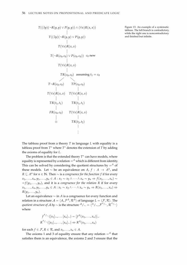
56 LECTURE NOTES ON PROPOSITIONAL AND PREDICATE LOGIC
T((∃y)(¬R(y, y) ∨ P(y, y)) ∧ (∀x)R(x, x))
T((∃y)(¬R(y, y) ∨ P(y, y))
T(∀x)R(x, x)
T(¬R(c0, c0) ∨ P(c0, c0)) c0 new
T(∀x)R(x, x)
TR(c0, c0) assuming t1 = c0
T¬R(c0, c0)
T(∀x)R(x, x)
TR(t1, t1)
FR(c0, c0)
⊗
TP(c0, c0)
T(∀x)R(x, x)
TR(t1, t1)
T(∀x)R(x, x)
TR(t2, t2)
...
Figure 13: An example of a systematictableau. The left branch is contradictory,while the right one is noncontradictoryand finished but infinite.
The tableau proof from a theory T in language L with equality is atableau proof from T∗ where T∗ denotes the extension of T by addingthe axioms of equality for L.
The problem is that the extended theory T∗ can have models, whereequality is represented by a relation =A which is different from identity.This can be solved by considering the quotient structures by =A ofthese models. Let ∼ be an equivalence on A, f : A → An, andR ⊆ An for n ∈N. Then ∼ is a congruence for the function f if for everyx1, . . . , xn, y1, . . . , yn ∈ A : x1 ∼ x2 ∧ · · · ∧ xn ∼ yn ⇒ f (x1, . . . , xn) ∼= f (y1, . . . , yn), and it is a congruence for the relation R if for everyx1, . . . , xn, y1, . . . , yn ∈ A : x1 ∼ x2 ∧ · · · ∧ xn ∼ yn ⇒ R(x1, . . . , xn)⇔R(y1, . . . , yn).
Let an equivalence ∼ in A is a congruence for every function andrelation in a structure A = ⟨A,FA,RA⟩ of language L = ⟨F ,R⟩. Thequotient structure of A by ∼ is the structure A/∼ = ⟨A/∼,F A/∼ ,RA/∼⟩where
fA/∼([x1]∼, . . . [xn]∼) = [ f A(x1, . . . , xn)]∼
RA/∼([x1]∼, . . . , [xn]∼)⇔ RA(x1, . . . , xn)
for each f ∈ F , R ∈ R, and x1, . . . , xn ∈ A.The axioms 1 and 3 of equality ensure that any relation =A that
satisfies them is an equivalence, the axioms 2 and 3 ensure that the
TABLEAU METHOD IN FIRST-ORDER LOGIC 57
relation is also a congruence. If we have a model A ⊨ T∗ then also(A/=A) ⊨ T∗. Moreover, equality is interpreted as identity in A/=A .
We can now prove the soundness of the tableau method in predicatelogic. The proof again closely resembles the one from the propositionallogic. We will in fact also use a similar lemma. We say that a modelA agrees with an entry P in a tableau if P is Tφ and A ⊨ φ or if P isFφ and A ⊨ ¬φ, i.e. A ⊭ φ. Moreover, A agrees with a branch V if Aagrees with every entry on V.
Lemma 5. Let A be a model of a theory T of a language L that agrees withthe root entry R in a tableau τ = ∪τn from T. Then A can be expanded to alanguage LC so that it agrees with some branch V in τ.
Proof. We prove the lemma by induction on n. We will find a branchVn in τn and an expansion An by constants cA for all c ∈ LC \ L on Vn
such that An agrees with Vn and Vn−1 ⊆ Vn.Assume we have a branch Vn in τn and an expansionAn that agrees
with Vn.
• If τn+1 is obtained from τn without extending the branch Vn, takeVn+1 = Vn and An+1 = An.
• If τn+1 is obtained from τn by appending Tφ for some φ ∈ T tothe end of Vn, let Vn+1 be the branch Vn with Tφ at the end andAn+1 = An. Since A ⊨ φ, An+1 agrees with Vn+1.
• Otherwise τn+1 is obtained from τn by appending an atomic tableaufor an entry P on Vn to Vn. By induction we know that A agreeswith P. If P is formed by a logical connective, we take An+1 = Aand verify that Vn can always be extended to Vn+1 (this is the sameas in propositional logic). If P is in form T(∀x)φ(x), let Vn+1 bethe unique extension of Vn to a branch τn+1 by the entry Tφ(x/t).Let An+1 be any expansion of An by new constants from t. SinceAn ⊨ (∀x)φ(x) also An+1 ⊨ φ(x/t). Analogously for P in formF(∃x)φ(x). Finally, if P is in form T(∃x)φ(x), let Vn+1 be the uniqueextension of Vn to a branch in τn+1, i.e. by the entry Tφ(x/c). SinceAn ⊨ (∃x)φ(x) there is some a ∈ A, such that A ⊨ φ(x)[e(x/a)]for every assignment e. Let An+1 be the expansion of An by a newconstant cA = a. Then An+1 ⊨ φ(x/c). Analogously for P in formF(∀x)φ(x).
The base step for n = 0 follows from the analysis of the atomic tableauxfor the root entry R applying the assumption thatA agrees with R.
We can finally prove the soundness of the tableau method in first-order logic. The proof is in fact almost identical to the one in proposi-tional logic.
Theorem 11. For every theory T and sentence φ, if φ is tableau provablefrom T, then φ is valid in T, i.e. T ⊢ φ⇒ T ⊨ φ.
Proof. Let φ be tableau provable from T, i.e. there is a contradictorytableau from T with root entry Fφ. Assume for contradiction that φ

58 LECTURE NOTES ON PROPOSITIONAL AND PREDICATE LOGIC
is not valid in T, i.e. there is a model A of T in which φ is not true.However, in such a case A agrees with the root entry Fφ of the proofand therefore by previous lemma it can be expanded to the languageLC so that it agrees with a branch in τ. But all the branches in τ arecontradictory, thus it is not possible.
Now, we would like to prove the completeness of the tableaumethod in first-order logic. We will again use the branch in a non-contradictory tableau and a model that agrees with the branch in orderto provide a counter-example. This time, the model will be so calledcanonical model. In the canonical model, the universe is formed byall the ground terms of the language and the representations of allfunction symbols is fixed. This means we can imagine the groundatomic formulas, informally, as complex names of propositional vari-ables and therefore the proof of completeness in principle reduces toits equivalent in the propositional logic.
Let V be a noncontradictory branch of a finished tableau from atheory T of a language L = ⟨F ,R⟩. The canonical model from V isthe LC-structure A = ⟨A,FA,RA⟩ where A is the set of all groundterms of the language LC, f A(t1, . . . , tn) = f (t1, . . . , tn) for every n-ary function symbol f ∈ F ∪ (LC \ L)16, and t1, . . . , tn ∈ A, and 16 The expression f (t1, . . . , tn) is a
ground term of the language andtherefore is in A.
RA(t1, . . . , tn) ⇔ TR(t1, . . . , tn) is an entry on V for every n-ary rela-tion symbol R ∈ R and every t1, . . . , tn ∈ A.
If L is with equality, T∗ is an extension of T by the axioms of equalityfor L. The equality will be interpreted in the model by some relation=A. We also have t1 =A t2 ⇔ T(t1 = t2) is an entry of V. SinceV contains all axioms of equality (it is finished), the relation =A isa congruence for all functions and relations in A. If we require thatthe equality is represented by identity, we take the quotient of thecanonical model A by the congruence =A. The canonical model withequality from V is the quotient A/=A .
Lemma 6. The canonical model A from a noncontradictory finished branchV agrees with V.
Proof. We will prove the lemma by induction on the structure of sen-tence φ in an entry on V.
• For atomic φ, if Tφ is on V then A ⊨ φ by definition. If Fφ is onV, then Tφ is not on V since V is noncontradictory, so A ⊨ ¬φ bydefinition.
• If T(φ ∧ ψ) is on V, then Tφ and Tψ are on V since V is finished.By induction A ⊨ φ and A ⊨ ψ, thus A ⊨ φ ∧ ψ. For other logi-cal connectives similarly (this step is the same as in the proof inpropositional logic).
• If T(∀x)φ(x) is on V, then Tφ(x/t) is on V for every term t ∈ Asince V is finished. By induction A ⊨ φ(x/t) for every t ∈ A andthus A ⊨ (∀x)φ(x). Similarly for F(∃x)φ(x) on V.

TABLEAU METHOD IN FIRST-ORDER LOGIC 59
• Finally, if T(∃x)φ(x) is on V, then Tφ(x/c) is on V for some c ∈ A.By induction, A ⊨ φ(x/c) and thus A ⊨ (∃x)φ(x). Similarly forF(∀x)φ(x) on V.
We can finally prove the completeness of the tableau method. Asalways, the proof is very similar to the one in propositional logic.
Theorem 12. For every theory T and sentence φ, if φ is valid in T, then φ
is tableau provable from T, i.e. T ⊨ φ⇒ T ⊢ φ.
Proof. Let φ is valid in T. We will show that an arbitrary finishedtableau τ from a theory T with the root entry Fφ is contradictory.Assume for a contradiction, that it is not, i.e. that there is a noncon-tradictory branch V in τ. By the previous lemma, there is a structureA for LC that agrees with V, in particular with the root entry Fφ, i.e.A ⊨ ¬φ. Let A′ be the reduct of A to the language L, then A′ ⊨ ¬φ.Since V is finished, it contains Tψ for every ψ ∈ T. Thus A′ is a modelof T. But this contradicts the assumption that φ is valid in T (φ is notvalid in the model A′ of the theory T). Therefore the tableau τ is aproof of φ from T.
As with propositional logic, we can again re-define the semanticalterms using syntactical notions. In fact, this and the next paragraphare copied from the propositional part with only minor changes. Firstof all, we define the set of theorems of L-theory T
ThmL(T) = {φ|φ ∈ FmL, T ⊢ φ} .
We say that a theory T is inconsistent, if T ⊢ ⊥, otherwise T is consistent.A theory T is complete, if it is consistent and every sentence is provableor refutable from T, i.e. if T ⊢ ¬φ or T ⊢ φ. A theory T in L is an exten-sion of T′ in L′, if L′ ⊆ L and ThmL′(T′) ⊆ ThmL(T), the extension issimple, if L = L′, and it is conservative if ThmL′(T′) = ThmL(T)∩ FmL′ .Two theories T and T′ are equivalent, if T is an extension of T′ and viceversa.
There are strong relations between the syntactic terms introducedabove and the semantic terms introduced in the previous chapter. Mostof these are corollaries of the soundness and completeness of tableaumethod. For each theory T and sentences φ, ψ of a language L
1. T ⊢ φ if and only if T ⊨ φ ,
2. ThmL(T) = θL(T) ,
3. T is inconsistent if and only if T is unsatisfiable, i.e. it has no model,
4. T is complete if and only if T is semantically complete, i.e. it has asingle model, up to elementary equivalence, and
5. (deduction theorem) T ∪ {φ} ⊢ ψ if and only if T ⊢ φ→ ψ .
A corollary of the proofs is the weak version of the Lövenheim-Skolem theorem.

60 LECTURE NOTES ON PROPOSITIONAL AND PREDICATE LOGIC
Theorem 13. Every consistent theory T of a countable language L withoutequality has a countably infinite model.
Proof. Let τ be the systematic tableau from T with F⊥ in the root.Since τ is consistent, ⊥ is not provable from T and therefore τ containsa noncontradictory branch V, and there exists a canonical model Afrom V (in language LC). Since A agrees with V its reduct to thelanguage L is the desired countably infinite model of T.
We needed the assumption that the theory is without equality be-cause the canonical model with equality can be also finite (but it isalways countable).
As in propositional logic, we can also prove the compactness theo-rem in first-order logic.
Theorem 14 (compactness). A theory T has a model if and only if everyfinite subset of T has a model.
Proof. The implication from left to right is obvious. For the otherimplication, if T has no model, then it is inconsistent, i.e. ⊥ is provableby a systematic tableau τ from T. Since τ is finite, ⊥ is provable fromsome finite T′ ⊆ T, i.e. T′ has no model.
The compactness theorem has an interesting corollary which givesus the so called non-standard model of natural numbers. Let N =
⟨N, S,+, ·, 0,≤⟩ be the standard model of natural numbers, and letTh(N) be the theory consisting of all sentences valid in N. For n ∈N,we denote n = S(S(S(S(...S(0))))) (n applications of the function S)the so called n-th numeral. Now, let us consider a theory T with a newconstant symbol c, such that T = Th(N) ∪ {n ⪇ c|n ∈ N}. Everyfinite subset of such theory has a model, therefore also the wholetheory T has a model. This is a non-standard model of natural numbers.Every sentence that is valid in Th(N) is also valid in this model, butit additionally contains an element that is greater than all naturalnumbers.
In mathematics, we very often define new functions or relationsusing formulas from the theory we work with. Now, we will showthat such definitions do not in any way increase the strength of thetheory, i.e. that by adding definitions of new symbols to a theory, weobtain a conservative extension of that theory. Before we get to thatpoint, we will show a simple lemma that gives us a simple way toshow that a theory is an (conservative) extension of another theory.
Lemma 7. Let T be a theory of L and T′ a theory of L′ where L ⊆ L′.
1. T′ is an extension of T if and only if the reduct A of every model A′ of T′
to the language L is a model of T,
2. T′ is a conservative extension of T, if T′ is an extension of T and everymodel A of T can be expanded to the language L′ on a model A′ of T′.
Proof. 1. If T′ is an extension of T and φ ∈ T then T′ ⊨ φ. ThusA′ ⊨ φ
and also A ⊨ φ, which implies that A is a model of T. On the other
TABLEAU METHOD IN FIRST-ORDER LOGIC 61
hand, if A is a model of T and T ⊨ φ for a φ of language L, thenA ⊨ φ and also A′ ⊨ φ. Therefore T′ ⊨ φ and T′ is an extension ofT.
2. If T′ ⊨ φ where φ is of the language L and A is a model of T, thenin its expansion A′ that is a model of T′ we have also A′ ⊨ φ. Thusalso A ⊨ φ, and hence T ⊨ φ. Therefore T′ is conservative.
We now start by showing that adding a definition of new rela-tion does not change the strength of the theory. Let T be a theoryof a language L and ψ(x1, . . . , xn) a formula of L with free variablesx1, . . . , xn. Let L′ denote the extension of the language L with a newn-ary relation symbol R. The extension of T by definition of R with aformula ψ is the theory T′ of L′ obtained from T by adding the axiomR(x1, . . . , xn)↔ ψ(x1, . . . , xn). Obviously, in such a case every modelof T can be uniquely expanded into a model of T′ and therefore T′
is a conservative extension of T. Moreover, we can “translate” eachformula φ′ of L′ into a formula φ of L such that T′ ⊨ φ′ ↔ φ. Wejust replace each sub-formula R(t1, . . . , tn) with ψ′(x1/t1, . . . , xn/tn),where ψ′ is a suitable variant of ψ (such that every substitution can beperformed).
Similarly, adding a definition of a function symbol does not in-crease the strength of the theory. Let T be a theory of a languageL, ψ(x1, . . . , xn, y) an L-formula with free variables x1, . . . , xn, y suchthat T ⊨ (∃y)ψ(x1, . . . , xn, y) (existence) and T ⊨ ψ(x1, . . . , xn, y) ∧ψ(x1, . . . , xn, z) → y = z (uniqueness). Let L′ be an extension ofL with a new n-ary function symbol f . The extension of T by defi-nition of f by the formula ψ is the theory T′ of L′ obtained from Tby adding the axiom f (x1, . . . , xn) = y ↔ ψ(x1, . . . , xn, y). Com-monly, ψ is t(x1, . . . , xn) = y for a term t and variables x1, . . . , xn.In such a case both existence and uniqueness always hold. Obvi-ously, every model of T can be uniquely extended to a model of T′
and therefore T′ is again a conservative extension of T. Moreover,we can again “translate” the formula φ′ in L′ into a formula φ in Lsuch that these two formulas are T′-equivalent (i.e. T′ ⊨ φ′ ↔ φ).We show the translation only for formulas that contain the functionf only once, for other formulas, we can repeat the process induc-tively. Let φ∗ denote the formula obtained from φ′ by replacingthe term f (t1, . . . , tn) with a new variable z. Let φ be the formula(∃z)(φ∗ ∧ ψ′(x1/t1, . . . , xn/tn, y/z), where ψ′ is a suitable variant of ψ.Now, ifA is a model of T′, e is an assignment, and a = f A(t1, . . . , tn)[e],by the two conditions, A ⊨ ψ′(x1/t1, . . . , xn/tn, y/z)[e] if and only ife(z) = a. Thus A ⊨ φ[e] ⇔ A ⊨ φ∗[e(z/a)] ⇔ A ⊨ φ′[e] for everyassignment e, i.e. A ⊨ φ′ ↔ φ and so T′ ⊨ φ′ ↔ φ.
The two previous paragraphs show that if we have a theory T′ of thelanguage L′ which was obtained from T of L by successive definitionsof relation and function symbols (extension of T by definitions) thenevery model of T can be uniquely expanded into a model of T′, T′ is aconservative extension of T, and for every formula φ′ of L′ there is aformula φ of L such that T′ ⊨ φ′ ↔ φ.


Resolution in First-Order Logic
We now aim to introduce the resolution method in predicate logic. Tothis end, we will need to show that the problem of satisfiability of the-ories can be reduced to open theories. We will show that every theoryhas an open conservative extension and therefore the satisfiability ofthe theory can be expressed as the satisfiability of the open extension.
We say that two theories T and T′ are equisatisfiable it T has a model ifand only if T′ has a model. A formula is in the prenex (normal) form(PNF) if it is written as (Q1x1) . . . (Qnxn)φ′, where Qi denotes ∀ or ∃and φ′ is an open formula called the matrix. (Q1x1) . . . (Qnxn) is theprenex. If all the quantifiers are ∀ then φ is a universal formula.
We obtain the equisatisfiable open theory T′ by first transformingall axioms of T into the prenex form. Then we remove the existentialquantifiers (we will create so called Skolem variant of the formula)thus obtaining a universal formula. The matrices of the universalformulas will be the axioms of T′.
Prenex Normal Form
We start by the transformation of formulas into the prenex normalform. The transformation is based on replacing some occurrences ofa sub-formula ψ in a formula φ by an equivalent sub-formula ψ′. Itis easy to show (by induction on the structure of formula φ) that theobtained formula is equivalent to φ.
Let Q denote ∀ or ∃ and Q denote the complementary quantifier.For every formulas φ and ψ such that x is not free in the formula ψ,the following equivalences (conversion rules) hold:
¬(Qx)φ↔ (Qx)¬φ
((Qx)φ ∧ ψ)↔ (Qx)(φ ∧ ψ)
((Qx)φ ∨ ψ)↔ (Qx)(φ ∨ ψ)
((Qx)φ→ ψ)↔ (Qx)(φ→ ψ)
(ψ→ (Qx)φ)↔ (Qx)(ψ→ φ)
All the equivalences can be proved by the tableau method. Theassumption that x is not free in ψ is necessary in each rule above.
By induction on the structure of formula φ, we can show that forevery formula φ there is an equivalent formula φ′ in the prenex normalform, i.e. ⊨ φ ↔ φ′. We just apply the conversion rules above (andreplace subformulas with suitable variants if needed).

64 LECTURE NOTES ON PROPOSITIONAL AND PREDICATE LOGIC
Skolem Variant
If the prenex of the formula contains only universal quantifiers (∀),we can remove them, thus obtaining an equivalent (and therefore alsoequisatisfiable) open formula. However, in many cases, some of thequantifiers will be existential. In such cases we can use the so calledSkolem variant as the equisatisfiable formula.
Let φ be a sentence of a language L in the prenex normal form,let y1, . . . , yn be the existentially quantified variables in φ (in this or-der), and for every i ≤ n let x1, . . . , xni be the universally quantifiedvariables in φ before yi. Let L′ be an extension of L with new ni-aryfunction symbols fi for all i ≤ n. Let φS denote the formula obtainedfrom φ by removing all the (∃yi) and replacing each occurrence of yi
by fi(x1, . . . , xni ). Then φS is the Skolem variant of φ.For example, for the formula
(∃y1)(∀x1)(∀x2)(∃y2)(∀x3)R(x1, y1, x2, y2, x3)
the Skolem variant is
(∀x1)(∀x2)(∀x3)R(x1, f1, x2, f2(x1, x2), x3) .
Informal! The new function symbols provide the witnesses for theexistentially quantified variables. We need a function, as these canbe different based on the previously universally quantified variables.That is also the reason, why the function have all the previouslyquantified variables as their parameters. The existentially quantifiedvariables do not need to be included in the parameters, as the functioncan “compute” them from the universally quantified ones.
We will now prove, that the Skolem variant φS of φ is equisatisfiablewith φ.
Lemma 8. Let φ be a sentence (∀x1) . . . (∀xn)(∃y)ψ of L and φ′ be a sen-tence (∀x1) . . . (∀xn)ψ(y/ f (x1, . . . , xn)) where f is a new function symbol.Then
1. the reduct A of every model A′ of φ′ to the language L is a model of φ,and
2. every model of φ can be expanded into a model A′ of φ′.
Proof. LetA′ ⊨ φ′ andA be the reduct ofA′ to L. SinceA ⊨ ψ[e(y/a)]for every assignment e where a = ( f (x1, . . . , xn)A
′)[e], we have also
A ⊨ φ.On the other hand, let A ⊨ φ. There is a function f A : An →
A such that for every assignment holds A ⊨ ψ[e(y/a)] where a =
f A(e(x1), . . . , e(xn)), and thus the expansion A′ of A by function f A
is a model of φ.
If φ′ is a Skolem variant of φ then both statements above also holdand therefore φ and φ′ are equisatisfiable.
It is important to realize that a formula and its Skolem variantare not equivalent. For example, φS ≡ (∀x)P(x, f (x)) is a Skolem

RESOLUTION IN FIRST-ORDER LOGIC 65
variant of φ ≡ (∀x)(∃y)P(x, y). Let A = ⟨{0, 1}, PA, f A⟩, wherePA = {(0, 0), (1, 1)} and f A(0) = 1, f A(1) = 0. Then A ⊨ φ, butA ⊭ φS. On the other hand, if φS is valid in a structure, φ also is, as fgives the y for which the formula holds, therefore, for a formula φ andits Skolem variant φS, we always have ⊨ φS → φ.
The difference between equivalence and equisatisfiability in thiscase is caused by the fact that the new functions in the Skolem variantare not in any way limited to cases where they provide the witnessesfor the existence and can therefore be defined arbitrarily, as we sawabove. If we defined the function in the “intended” way (in this case asthe identity on A), the Skolem variant would hold in such a structure.Therefore, it is also satisfiable.
The transformation to prenex normal form and the following cre-ation of Skolem variant gives us the possibility to reduce the questionof satisfiability to open theories, i.e. for every theory, there is an eq-uisatisfiable open theory. This is a corollary of the so called Skolemtheorem.
Theorem 15 (Skolem). Every theory T has an open conservative extensionT∗.
Proof. We assume T is in closed form (otherwise we can take theuniversal closures of all the axioms of T), and let L be its language.We first replace each axiom of T by an equivalent formula in prenexnormal form, thus obtaining theory T◦. Next, we replace each axiomin T◦ by its Skolem variant, which gives us a theory T′ in a languageL′ ⊇ L. Since every reduct of every model of T′ to L is a model of T, T′
is an extension of T. Furthermore, every model of T can be expandedto a model of T′ and therefore T′ is a conservative extension of T.Every axiom of T′ is a universal sentence, therefore we can take thematrices of these sentences to obtain an open theory T◦ equivalent toT′. T◦ is the open conservative extension of T.
Herbrand Model
We can even reduce the problem of satisfiability to propositional logicand show that if an open theory is unsatisfiable, we can demonstrateit via ground terms. For example, in the language L = ⟨P, R, f , c⟩ thetheory T = {P(x, y) ∨ R(x, y),¬P(c, y),¬R(x, f (x))} is unsatisfiablebecause the following conjunction of finitely many ground instancesof axioms of T is unsatisfiable:
P(c, f (c)) ∨ R(c, f (c)) ∧ ¬P(c, f (c)) ∧ ¬R(c, f (c)) .
This can also be seen as a unsatisfiable propositional formula (p ∨ r) ∧¬p ∧ ¬r.
A ground instance of formula φ with free variables x1, . . . , xn isφ(x1/t1, . . . , xn/tn) where t1, . . . , tn are ground terms.
The reduction of satisfiability to propositional logic is done usingthe notion of Herbrand models. Let L = ⟨R,F⟩ be a language withat least one constant symbol (we can add a new constant symbol, if
66 LECTURE NOTES ON PROPOSITIONAL AND PREDICATE LOGIC
needed). The Herbrand universe for L is the set of all ground termsof L. An L-structure A is a Herbrand structure, if its domain A is theHerbrand universe for L and for each n-ary function symbol f ∈ F ,t1, . . . , tn ∈ A, f A(t1, . . . , tn) = f (t1, . . . , tn). A Herbrand model of atheory T is a Herbrand structure that is a model of T.
We can see, that the definition of the Herbrand universe and ofthe function symbols in the Herbrand structure is the same as inthe canonical model, however, Herbrand structures do not specifythe relations. This is important, as every canonical model is also aHerbrand model.
The reduction of unsatisfiability to propositional logic is formallygiven by the Herbrand’s theorem.
Theorem 16 (Herbrand). Let T be an open theory of a language L withoutequality and with at least one constant symbol, then either T has a Herbrandmodel, or there are finitely many ground instances of axioms of T whoseconjunction is unsatisfiable, and thus T has no model.
Proof. Let T′ be the set of all ground instances of axioms of T. Considera finished systematic tableau τ from T′ in the language L (withoutadding new constant symbols) with the root entry F⊥. If the tableau τ
contains a noncontradictory branch V, the canonical model from V is aHerbrand model. Otherwise, τ is contradictory, i.e. T′ ⊢ ⊥. Thereforeτ is also finite and ⊥ is provable from finitely many formulas of T′, i.e.their conjunction is unsatisfiable.
The Herbrand model also works in languages L with equality, wejust need to take the extension T∗ of T with the axioms of equality andif T∗ has a Herbrand model A we take its quotient by =A.
A corollary of the Herbrand’s theorem is that an open theory T of alanguage L with at least one constant symbol is satisfiable if and onlyif the theory T′ of all ground instances of axioms of T is satisfiable.Why? If T has a model A, every instance of each axiom of T is validin A, and thus A is also a model of T′. If T is unsatisfiable then byHerbrand theorem there are finitely ground instances of axioms of Tthat are not satisfiable and therefore T′ is also unsatisfiable.
Another corollary says that for every open φ(x1, . . . , xn) of a lan-guage L with at least one constant symbol, the formula (∃x1) . . . (∃xn)φ
is valid if and only if there exist mn ground terms tij of L for somem such that φ(x1/t11, . . . , xn/t1n) ∨ · · · ∨ φ(x1/tm1, . . . , xn/tmn) is atautology. We know that (∃x1) . . . (∃xn)φ is valid if and only if itsnegation (∀x1) . . . (∀xn)(¬φ) is unsatisfiable, which is equivalent to¬φ being unsatisfiable. The Herbrand theorem for {¬φ} gives usfinitely many (m) ground instances of {¬φ} such that their conjunc-tion ψ is unsatisfiable. The negation of ψ is the desired tautology.
We will now discuss the resolution method in predicate logic. Itis again a refutation procedure, i.e. it aims to show that a formula ortheory are not satisfiable. It assumes the formulas are open and inCNF. These are then represented in the clausal form as in propositionallogic. Now, literals are atomic formulas and their negations, a clauseis a finite set of literals (□ denotes the empty clause) and a formula in

RESOLUTION IN FIRST-ORDER LOGIC 67
clausal form is a set of clauses. The resolution rule in first-order logic isbased on the rule in propositional logic, but is more general – it allowsto resolve through literals that are different, if they are unifiable (i.e. ifthere is such a substitution that they become identical). Resolution infirst-order logic is thus based on the resolution in propositional logicand unification.
Resolution
The Herbrand’s theorem actually gives us an (ineffective) way, howto perform the resolution in first-order logic. If we have an inputformula S in clausal form and we assume the language has at leastone constant symbol, we can create the set S′ of all ground instancesof all clauses in S. If we now consider the atomic sentences as namesof propositional variables, we may view S′ as a propositional formulain clausal form. We may now verify that it is unsatisfiable using thepropositional version of the resolution method. While this method inprinciple works, it is very inefficient, as we need to work with largenumbers of ground instances. Therefore, instead of grounding, we usesuitable substitutions in order to perform the resolution on as generalclauses as possible.
A substitution is a finite set σ = {x1/t1, . . . , xn/tn}, where xi, i ≤ nare distinct variables, ti are terms and the term ti is not xi. If all ti areground terms, σ is a ground substitution, if ti are distinct variables, σ
is a renaming of variables. An instance of an expression E by substitutionσ = {x1/t1, . . . , xn/tn} is the expression Eσ obtained from E by simul-taneously replacing all occurrences of xi by ti. For a set S of expressions,let Sσ = {Eσ|E ∈ S}. For two substitutions σ = {x1/t1, . . . , xn/tn}and τ = {y1/s1, . . . , ym/sm} we define the composition of σ and τ
as στ = {xi/tiτ|xi ∈ X, tiτ is not xi} ∪ {yj/sj|yj ∈ Y \ X} whereX = {x1, . . . , xn} and Y = {y1, . . . , ym}. For every expression E andsubstitutions σ, τ, ρ it holds (without proof) that (Eσ)τ = E(στ) and(στ)ρ = σ(τρ).
A unification is a special substitution. Let S = {E1, . . . , En} be afinite set of expressions. A unification for S is a substitution σ suchthat E1σ = E2σ = · · · = Enσ, i.e. Sσ is a singleton. We say that S isunifiable, if S has a unification. A unification σ of S is a most generalunification (mgu) if for every unification τ of S there is a substitution λ
such that τ = σλ. Obviously, if σ and τ are two different most generalunifications of S, they differ only in renaming of variables.
The general resolution rule in first-order logic is then defined inthe following way: let C1, C2 be clauses with distinct variables suchthat C1 = C′1 ⊔ {A1, . . . , An} and C2 = C′2 ⊔ {¬B1, . . . ,¬Bm}, let σ bea most general unifier of S = {A1, . . . , An, B1, . . . , Bm}. The resolventof C1 and C2 is C = C′1σ ∪ C′2σ.
For example, in clauses {P(x), Q(x, z)} and {¬P(y),¬Q( f (y), y)}we can unify S = {Q(x, z), Q( f (y), y)} applying the most general uni-fication σ = {x/ f (y), z/y} and resolve to a clause {P( f (y)),¬P(y)}.
The resolution proof and related notions are then defined in almost

68 LECTURE NOTES ON PROPOSITIONAL AND PREDICATE LOGIC
the same way as in propositional logic. Resolution proof (deduction)of a clause C from a formula S is a finite sequence C0, . . . , Cn = C,such that for every i ≤ n, we have Ci = C′i σ form some C′i ∈ Sand a renaming of variables σ, or Ci is a resolvent of some previousclauses. A clause C is (resolution) provable from S (S ⊢R C), if it hasa resolution proof from S. A refutation of a formula S is a resolutionproof of □ from S. S is resolution refutable if S ⊢R □.
It remains to show how to find the most general unifications weneed in the resolution method. There is in fact a simple algorithm tofind them: let S be a finite set of expressions and p be the leftmostposition in which some expressions of S differ. Then the difference inS is the set D(S) of subexpressions of all expressions of S starting atthe position p. For example S = {P(x, y), P(( f (x), z), P(z, f (x)} hasD(S) = {x, f (x), z}.
The input of the algorithm is a nonempty finite set of expressions S,its output is the most general unification σ of S or information that Sis not unifiable. The algorithm performs the steps bellow:
1. Let S0 ← S, σ0 ← ∅, k← 0.
2. If Sk is a singleton, output the substitution σ = σ0σ1 . . . σk.
3. If D(Sk) contains a variable x and a term t with no occurrence of x,let σk+1 ← {x/t}, Sk+1 ← Skσk+1, k← k + 1 and go to step 2.
4. Otherwise output “S is not unifiable”.
The occurrence check in step 3 can be expensive and slows thealgorithm down significantly. Therefore some implementations (e.g.those in most Prolog interpreters) ignore that. However, it can lead toinfinite loops.
We now show the correctness of the unification algorithm – theunification algorithm outputs a correct answer in finite time for anyinput S, i.e. a most general unification σ of S or it detects that S isnot unifiable. The algorithm eliminates one variable in each iteration,therefore it finishes in finite time. If it ends negatively after k iterations,D(Sk) is not unifiable and therefore also S is not. If it outputs σ =
σ0σ1 . . . σk, clearly σ is a unification of S. We only need to show it is amost general one, i.e. for every unification τ of S there is a substitutionλ such that τ = σλ. We will show that in this case, λ = τ and thereforeτ = στ (this property will also be important in the proof of liftinglemma later, let us call this property (*)). Let τ be a unification ofS, we will show that τ = σ0σ1 . . . σiτ for every i ≤ k. It obviouslyholds for k = 0. Let σi+1 = {x/t} and assume τ = σ0σ1 . . . σiτ. Itsuffices to show that vσi+1τ = vτ for every variable τ. If v = x,vσi+1 = v and it holds. Otherwise v = x and vσi+1 = xσi+1 = t. Sinceτ unifies Si = Sσ0σ1 . . . σi and both the variable x and term t are inD(Si) (otherwise σi+1 would be different), τ has to unify x and t, i.e.tτ = xτ as required.
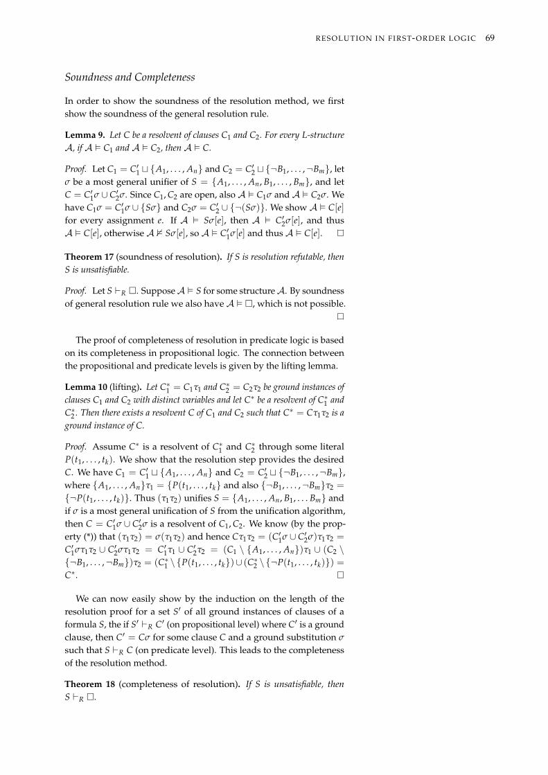
RESOLUTION IN FIRST-ORDER LOGIC 69
Soundness and Completeness
In order to show the soundness of the resolution method, we firstshow the soundness of the general resolution rule.
Lemma 9. Let C be a resolvent of clauses C1 and C2. For every L-structureA, if A ⊨ C1 and A ⊨ C2, then A ⊨ C.
Proof. Let C1 = C′1 ⊔ {A1, . . . , An} and C2 = C′2 ⊔ {¬B1, . . . ,¬Bm}, letσ be a most general unifier of S = {A1, . . . , An, B1, . . . , Bm}, and letC = C′1σ ∪ C′2σ. Since C1, C2 are open, also A ⊨ C1σ and A ⊨ C2σ. Wehave C1σ = C′1σ ∪ {Sσ} and C2σ = C′2 ∪ {¬(Sσ)}. We show A ⊨ C[e]for every assignment e. If A ⊨ Sσ[e], then A ⊨ C′2σ[e], and thusA ⊨ C[e], otherwise A ⊭ Sσ[e], so A ⊨ C′1σ[e] and thus A ⊨ C[e].
Theorem 17 (soundness of resolution). If S is resolution refutable, thenS is unsatisfiable.
Proof. Let S ⊢R □. SupposeA ⊨ S for some structureA. By soundnessof general resolution rule we also have A ⊨ □, which is not possible.
The proof of completeness of resolution in predicate logic is basedon its completeness in propositional logic. The connection betweenthe propositional and predicate levels is given by the lifting lemma.
Lemma 10 (lifting). Let C∗1 = C1τ1 and C∗2 = C2τ2 be ground instances ofclauses C1 and C2 with distinct variables and let C∗ be a resolvent of C∗1 andC∗2 . Then there exists a resolvent C of C1 and C2 such that C∗ = Cτ1τ2 is aground instance of C.
Proof. Assume C∗ is a resolvent of C∗1 and C∗2 through some literalP(t1, . . . , tk). We show that the resolution step provides the desiredC. We have C1 = C′1 ⊔ {A1, . . . , An} and C2 = C′2 ⊔ {¬B1, . . . ,¬Bm},where {A1, . . . , An}τ1 = {P(t1, . . . , tk} and also {¬B1, . . . ,¬Bm}τ2 =
{¬P(t1, . . . , tk)}. Thus (τ1τ2) unifies S = {A1, . . . , An, B1, . . . Bm} andif σ is a most general unification of S from the unification algorithm,then C = C′1σ ∪ C′2σ is a resolvent of C1, C2. We know (by the prop-erty (*)) that (τ1τ2) = σ(τ1τ2) and hence Cτ1τ2 = (C′1σ ∪ C′2σ)τ1τ2 =
C′1στ1τ2 ∪ C′2στ1τ2 = C′1τ1 ∪ C′2τ2 = (C1 \ {A1, . . . , An})τ1 ∪ (C2 \{¬B1, . . . ,¬Bm})τ2 = (C∗1 \ {P(t1, . . . , tk})∪ (C∗2 \ {¬P(t1, . . . , tk)}) =C∗.
We can now easily show by the induction on the length of theresolution proof for a set S′ of all ground instances of clauses of aformula S, the if S′ ⊢R C′ (on propositional level) where C′ is a groundclause, then C′ = Cσ for some clause C and a ground substitution σ
such that S ⊢R C (on predicate level). This leads to the completenessof the resolution method.
Theorem 18 (completeness of resolution). If S is unsatisfiable, thenS ⊢R □.

70 LECTURE NOTES ON PROPOSITIONAL AND PREDICATE LOGIC
Proof. If S is unsatisfiable that by the corollary of Herbrand’s theoremalso the set S′ of all ground clauses is unsatisfiable. By completenessof resolution in propositional logic, S′ ⊢R □. By the above paragraph,there is a clause C and a ground substitution σ such that □ = Cσ andS ⊢R C. But the only clause that has □ as a ground instance is theclause C = □.
This concludes the part of the lecture dedicated to the predicatelogic. We closely followed the previous part on propositional logic andextended the ideas to the first-order logic. The differences are mostlygiven by the more expressive language of predicate logic. We againstarted the discussion with syntax and semantics, we saw that modelsin first order logic are structures. Then, we showed two formal proofmethods – tableau method and resolution.
In the next (and last) part, we will first discuss the basics of modeltheory and then we will show the limits of the formal systems.
Part III
Model Theory andIncompleteness


Basics of model theory and decidability
In the last part of the lecture, we will discuss the basics of modeltheory, decidability of theories and the incompleteness of some the-ories. Model theory is a rather modern branch of logic that rapidlydeveloped in the 1990s. As its name suggests, it studies the modelsof theories and answers (among others) questions like: what is thenumber of models of a theory T up to isomorphisms, is the theory Tcomplete, etc.
The decidability of theories deals with the problem if we can algo-rithmically decide whether a sentence is provable in a theory T or not.If it is, the theory is called decidable.
Finally, we will discuss the so called Gödel incompleteness theoremsthat state that once a theory is sufficiently strong, it is incomplete. Wewill also show that truth cannot be defined in logic.
Model Theory
We have actually already seen some terms that are considered a partof model theory. For example, we know that two structures are ele-mentarily equivalent if they satisfy the same sentences. We have alsodefined the theory of a structure A – Th(A) as the set of all sentencesvalid in A. This set is also a theory (it is a set of formulas). Moreover,Th(A) is always a complete theory, if A ⊨ T, then Th(A) is a simple(complete) extension of T, and if A ⊨ T and T is complete, then Th(A)is equivalent to T, i.e. Th(A) = θL(T). We can also easily see thatfor every models A,B of a theory T, A ≡ B if and only if Th(A) andTh(B) are equivalent theories.
Before we discuss some of the ideas of model theory further, wedefine some common algebraic theories.
1. the theory of groups in the language L = ⟨+,−, 0⟩ with equality hasaxioms
x + (y + z) = (x + y) + z
0 + x = x = x + 0
x + (−x) = 0 = (−x) + x
2. the theory of Abelian groups has moreover the axiom x + y = y + x

74 LECTURE NOTES ON PROPOSITIONAL AND PREDICATE LOGIC
3. the theory of rings in L = ⟨+,−, ·, 0, 1⟩ has moreover axioms
1 · x = x = x · 1x · (y · z) = (x · y) · zx · (y + z) = x · y + x · z(x + y) · z = x · z + y · z
4. the theory of commutative rings has moreover the axiom x · y = y · x,and
5. the theory of fields in the same language has additional axioms
x = 0→ (∃y)(x · y = 1)
0 = 1
Another important theory is the theory of dense linear orders DeLO∗
of the language L = ⟨≤⟩ with equality that has axioms
x ≤ x
x ≤ y ∧ y ≤ x → x = y
x ≤ y ∧ y ≤ z→ x ≤ z
x ≤ y ∨ y ≤ x
x < y→ (∃x)(x < z ∧ z < y)
(∃x)(∃y)(x = y)
where x < y means x ≤ y∧ x = y. Let φ be the sentence (∃x)(∀y)(x ≤y) and let ψ be the sentence (∃x)(∀y)(y ≤ x). We will see that DeLO∗
has the following four simple complete extensions (and none other):
DeLO = DeLO∗ ∪ {¬φ,¬ψ}DeLO+ = DeLO∗ ∪ {¬φ, ψ}DeLO− = DeLO∗ ∪ {φ,¬ψ}DeLO± = DeLO∗ ∪ {φ, ψ}
We already know the Lövenheim-Skolem theorem – let T be a con-sistent theory of a countable language L. If L is without equality, thenT has a countably infinite model. If L is with equality, then T has amodel that is countable (finite or countably infinite).
A corollary of the theorem is that for every structure A of a count-able language without equality, there exists a countably infinite struc-ture B such that A ≡ B. Why? We know that Th(A) is consistentsince it has a model A and by the Lövenheim-Skolem theorem it hasa countably infinite model B. Since Th(A) is complete A must beelementarily equivalent to B.
Similarly for theories in language with equality, but we additionallyneed the assumption that A is infinite: for every infinite structure A ofa countable language without equality, there exists a countably infinitestructure B such that A ≡ B. The proof is similar to the one above.This time we also know that the sentence “there are exactly n elements”

BASICS OF MODEL THEORY AND DECIDABILITY 75
is not valid in A for any n and therefore also not in B and therefore Bmust be infinite.
These corollaries are quite strong, as is demonstrated in the follow-ing proof of existence of a countable algebraically closed field. We saythat a field A is algebraically closed if every polynomial (of non-zerodegree) has a root in A, i.e. we have for each n ∈N
A ⊨ (∀xn−1) . . . (∀x0)(∃y)(yn + xn−1 · yn−1 + · · ·+ x1 · y + x0 = 0) .
For example, the field C = ⟨C,+,−, ·, 0, 1⟩ of complex numbersis algebraically closed, while the fields of real numbers R or rationalnumbers Q are not. But since C is closed and infinite, by the previouscorollary, there is a countable structure elementarily equivalent to C
and therefore also algebraically closed.We now want to introduce the ω-categorical criterium of complete-
ness. To this end, we first need to define what is an isomorphism ofstructures. Let A and B be structures of a language L = ⟨F ,R⟩.A bijection h : A → B is a isomorphism of structures A and B ifboth h( f A(a1, . . . , an)) = f b(h(a1), . . . , h(an)) for every n-ary func-tion symbol f ∈ F and every a1, . . . , an ∈ A, and RA(a1, . . . , an) ⇔RB(h(a1), . . . , h(an)) for every n-ary relation symbol R ∈ R and everya1, . . . , an ∈ A. We say that A and B are isomorphic (via h) (A ≃ B) ifthere is an isomorphism h of A and B. We also say that A is isomor-phic with B. An automorphism of a structure A is an isomorphism ofA with A.
It is easy to show that isomorphisms preserve semantics, i.e. let Aand B be structures of a language L = ⟨F ,R⟩, a bijection h : A → Bis an isomorphism of A and B if and only if both h(tA[e]) = tB[he] forevery term t and e : Var → A, and A ⊨ φ[e] ⇔ B ⊨ φ[he] for everyformula φ and e : Var → A. This gives us a corollary that for everystructures A and B of the same language A ≃ B ⇒ A ≡ B, i.e. iftwo structures are isomorphic, they are also elementarily equivalent.The other implication does not generally hold, as we can have twoelementarily equivalent structures (e.g. the field of complex numbers C
and the countable algebraically closed field from the previous example)that are elementarily equivalent and not isomorphic (because theyhave different cardinality). However, the following lemma shows thatthe implication holds for finite structures in a language with equality.
Lemma 11. For every finite structures A and B of a language with equalityA ≡ B ⇒ A ≃ B.
Proof. First of all, we can see that |A| = |B| as the sentence “there areexactly n elements can be expressed in L”. For a finite language L,we can write a formula φ that defines A up to isomorphism17. This 17 The sentence says “there are exactly
n elements a1, . . . , an satisfying exactlythose atomic formulas on function val-ues and relations that are valid in thestructure A”.
formula holds both in A and B since they are elementarily equivalentand therefore they are also isomorphic.
For an infinite language L: there is only finite number of bijectionsbetween A and B, assume for contradiction, that none of them is anisomorphism. For each bijection hi choose a relation Ri in L that is notpreserved in this bijection. Let L′ ⊆ L is the language that contains

76 LECTURE NOTES ON PROPOSITIONAL AND PREDICATE LOGIC
only these relations. Obviously L′ is finite. Then the reducts of A andB to L′ are elementarily equivalent and therefore isomorphic (by theprevious paragraph) which is a contradiction.
A corollary of this lemma is that if a complete theory T in a languagewith equality has a finite model, then all models of T are isomorphic.
An isomorphic spectrum of a theory T is given by the number I(κ, T)of mutually non-isomorphic models of T for every cardinality κ. Atheory T is κ-categorical if it has exactly one model of cardinality κ (upto isomorphism), i.e. I(κ, T) = 1.
For example, the theory DeLO is ω-categorical. Let A,B ⊨ DeLO,with A = {ai}i∈N and B = {bi}i∈N. By induction on n we canfind injective hn ⊆ hn+1 ⊂ A× B preserving the ordering such that{ai}i<n ⊆ dom(hn) and {bi}i<n ⊆ rng(hn). Then A ≃ B via h = ∪hn.
Similarly, we obtain that A = ⟨Q,≤⟩,A ↾ [0, 1),A ↾ (0, 1], andA ↾ [0, 1] are up to isomorphism all countable models of DeLO∗.Therefore
I(κ, DeLO∗) =
{0 if κ ∈N ,4 if κ = ω .
This finally leads to the ω-categorical criterium of completeness(similar criteria also hold for cardinalities bigger than ω):
Theorem 19. Let L be at most countable language.
1. If a theory T in L without equality is ω-categorical, it is complete.
2. If a theory T in L with equality is ω-categorical and without finite models,it is complete.
Proof. Every model of T is elementarily equivalent with some count-ably infinite model of T, but such model is unique up to isomorphism,therefore all models of T are elementarily equivalent and T is com-plete.
The fact that isomorphisms preserve semantics also gives us a sim-ple condition for sets that can be defined in structures. The set de-fined by a formula φ(x, y) in structure A from parameters b ∈ A|b|is φA,b(x, y) = {a ∈ A|x||A ⊨ φ[e(x/a, y/b}. A set D ⊆ An is defin-able in the structure A from parameters b ∈ A|y| if there is a formulaφ(x, y), such that D = φA,b(x, y). It is easy to show, that definable setsmap to themselves in automorphism.
Lemma 12. Let D ⊆ An is a set definable in the structure A from parame-ters b and h is an automorphism on A identical on b. Then h[D] = D.
Proof. Let D = φA,b(x, y), then for every a ∈ An we have a ∈ D ⇔A ⊨ φ[e(x/a, y/b)] ⇔ φ[e ◦ h(x/a, y/b)] ⇔ φ[e(x/h(a), y/h(b))] ⇔φ[e(x/h(a), y/b)]⇔ h(a) ∈ D.
Decidability
Now, we would like to know if a given problem is algorithmicallydecidable (e.g. if a sentence is provable in a theory). We can formally

BASICS OF MODEL THEORY AND DECIDABILITY 77
define the notion of algorithm, for example using Turing machines.Decision problems can then be encoded into sets of natural numberscorresponding to the positive instances (with answer “yes”). Forexample, SAT = {⌈φ⌉|φ is a satisfiable formula }, where ⌈φ⌉ is thenatural number representing the formula φ. We say that a set A ⊆N isrecursive, if there is an algorithm that for every input x ∈N halts (stops)and correctly tells whether or not x ∈ A. We say that such algorithmdecides x ∈ A. We say that a set A ⊆ N is recursively enumerable ifthere is an algorithm that for every input x ∈ N halts if and only ifx ∈ A. We say that such algorithm recognizes x ∈ A. Equivalently,A is recursively enumerable if there is an algorithm that generates(enumerates) all elements of A.
Lemma 13. For every A ⊆ N A is recursive if and only if both A and Arecursively enumerable.
Proof. (⇒) If A is recursive, there is an algorithm that always haltsand returns whether x ∈ A. We can make an algorithm that halts onlyif x ∈ A (check if x ∈ A, if it is halt, otherwise enter an infinite loop).Therefore A is recursively enumerable. Similarly for A.
(⇐) If both A and A are recursively enumerable, there are twoalgorithms P1 and P2 such that P1 recognizes x ∈ A and P2 recognizesx ∈ A. We can start both these algorithms in parallel (make one stepof P1, then one step of P2, then another step of P1 and so on). For eachx ∈N, one of these algorithms eventually halts. If P1 halts first x ∈N,otherwise x /∈N. Therefore A (and also A) is recursive.
In logic, we are especially interested if a given theory is algorithmi-cally decidable. We assume a recursive language L. A theory T of L isdecidable, if Thm(T) is recursive, otherwise T is undecidable. It means, atheory is decidable, if there is an algorithm that for each sentence φ
decides whether T ⊢ φ or not.For every theory T of L with recursively enumerable axioms, Thm(T)
is recursively enumerable – the construction of systematic tableau fromT with root Fφ assumes a given enumeration of axioms of T. SinceT has recursively enumerable axioms, the construction provides analgorithm that recognizes T ⊢ φ.
If the theory T from the previous paragraph is additionally com-plete, then Thm(T) is recursive, i.e. T is decidable. Similarly to theproof of the lemma above, we can start the construction of systematictableaux from T with roots Fφ and Tφ. Since T is complete, then T ⊬ φ
if and only if T ⊢ ¬φ for every sentence φ. The construction thusprovides an algorithm that decides T ⊢ φ.
We now know that complete theories (with recursively enumerableaxioms) are decidable, however, completeness is a rather strong as-sumption. In fact, it is enough, if all the simple complete extensions ofa theory T are recursively enumerable, i.e. if there is an algorithm α(i, j)that generates the i-th axiom of th j-th extension (in some enumeration)or announces that such axiom does not exist.
So, if a theory T has recursively enumerable axioms and the set ofall simple complete extensions of T is recursively enumerable, then T
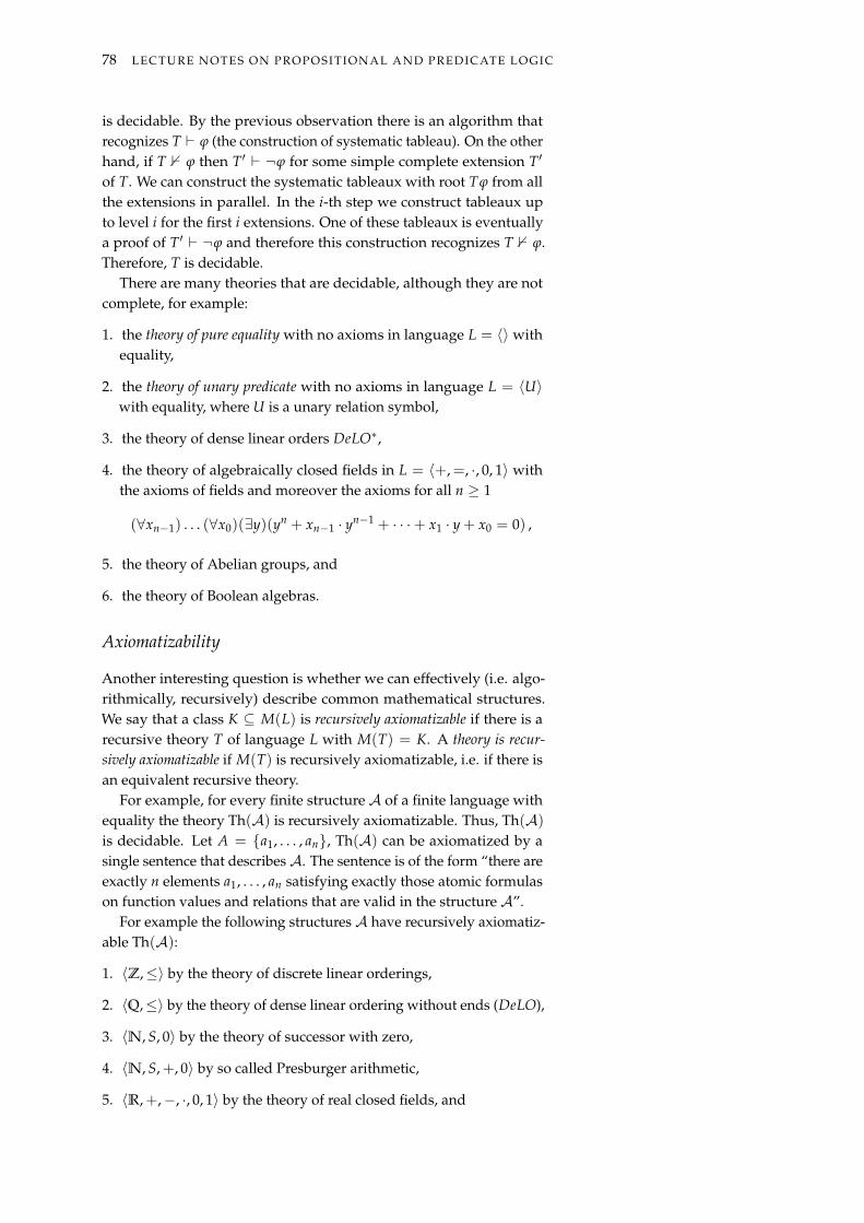
78 LECTURE NOTES ON PROPOSITIONAL AND PREDICATE LOGIC
is decidable. By the previous observation there is an algorithm thatrecognizes T ⊢ φ (the construction of systematic tableau). On the otherhand, if T ⊬ φ then T′ ⊢ ¬φ for some simple complete extension T′
of T. We can construct the systematic tableaux with root Tφ from allthe extensions in parallel. In the i-th step we construct tableaux upto level i for the first i extensions. One of these tableaux is eventuallya proof of T′ ⊢ ¬φ and therefore this construction recognizes T ⊬ φ.Therefore, T is decidable.
There are many theories that are decidable, although they are notcomplete, for example:
1. the theory of pure equality with no axioms in language L = ⟨⟩ withequality,
2. the theory of unary predicate with no axioms in language L = ⟨U⟩with equality, where U is a unary relation symbol,
3. the theory of dense linear orders DeLO∗,
4. the theory of algebraically closed fields in L = ⟨+,=, ·, 0, 1⟩ withthe axioms of fields and moreover the axioms for all n ≥ 1
(∀xn−1) . . . (∀x0)(∃y)(yn + xn−1 · yn−1 + · · ·+ x1 · y + x0 = 0) ,
5. the theory of Abelian groups, and
6. the theory of Boolean algebras.
Axiomatizability
Another interesting question is whether we can effectively (i.e. algo-rithmically, recursively) describe common mathematical structures.We say that a class K ⊆ M(L) is recursively axiomatizable if there is arecursive theory T of language L with M(T) = K. A theory is recur-sively axiomatizable if M(T) is recursively axiomatizable, i.e. if there isan equivalent recursive theory.
For example, for every finite structure A of a finite language withequality the theory Th(A) is recursively axiomatizable. Thus, Th(A)is decidable. Let A = {a1, . . . , an}, Th(A) can be axiomatized by asingle sentence that describes A. The sentence is of the form “there areexactly n elements a1, . . . , an satisfying exactly those atomic formulason function values and relations that are valid in the structure A”.
For example the following structures A have recursively axiomatiz-able Th(A):
1. ⟨Z,≤⟩ by the theory of discrete linear orderings,
2. ⟨Q,≤⟩ by the theory of dense linear ordering without ends (DeLO),
3. ⟨N, S, 0⟩ by the theory of successor with zero,
4. ⟨N, S,+, 0⟩ by so called Presburger arithmetic,
5. ⟨R,+,−, ·, 0, 1⟩ by the theory of real closed fields, and

BASICS OF MODEL THEORY AND DECIDABILITY 79
6. ⟨C,+,−, ·, 0, 1⟩ by the theory of algebraically closed fields withcharacteristic 0.
By the previous observation, for all the above structures A, the theoryTh(A) is decidable.
Apart from the recursive axiomatizability, we may also be interestedif a class of structures can be axiomatized by theories with other prop-erties. For example, a class K ⊆ M(L) is openly axiomatizable, if there isan open theory T, such that M(T) = K. A theory is openly axiomatizable,if M(T) is openly axiomatizable. We already know that if T is openlyaxiomatizable then every substructure of its model is also its model.The other implication also holds and gives a useful criterium to test ifa theory is openly axiomatizable. For example, the DeLO theory is notopenly axiomatizable, because a finite substructure of its model is notits model.
Another interesting case is finite axiomatizability. A class of struc-tures K ⊆ M(L) is finitely axiomatizable, if there is a finite theory T suchthat M(T) = K. Similarly, a theory T is finitely axiomatizable, if M(T) isfinitely axiomatizable. We again have a criterium to test if a class isfinitely axiomatizable.
Theorem 20. Let K ⊆ M(L), K = M(L) \ K, where L is a language. ThenK is finitely axiomatizable, if and only if both K and K are axiomatizable.
Proof. (⇒) If T is a finite axiomatization of K then the theory with asingle sentence
⋁φ∈T ¬φ axiomatizes K.
(⇐) Let T, S are theories of L such that M(T) = K, M(S) = K.Then M(S ∪ T) = M(T) ∩M(S) = ∅, by compactness, there are finitetheories T′ ⊆ T and S′ ⊆ S such that M(S′ ∪ T′) = ∅. Then M(T) ⊆M(T′) ⊆ M(S′) ⊆ M(S) = M(T) and therefore M(T) = M(T′).
There are actually classes of structures that are not axiomatizable atall. The compactness theorem gives us the following lemma:
Lemma 14. If a theory T has for each n ∈ N at least n-element model, ithas an infinite model.
Proof. For languages without equality this is true by the Lövenheim-Skolem theorem. In languages with equality, we create an extension T′
of T, such that T′ = T ∪ {ci = cj|i = j} in a language with countablymany new constant symbols ci. Every finite part of T′ has a modelaccording to the assumption and therefore T′ also has a model accord-ing to the compactness theorem. This model must be infinite, and itsreduct to the original language is the desired infinite model of T.
However, that means that if a theory has for each n ∈ N at leastn-element model, the class of its finite models is not axiomatizable,e.g. the class of finite groups of finite fields are not axiomatizable infirst-order logic.

80 LECTURE NOTES ON PROPOSITIONAL AND PREDICATE LOGIC
Incompleteness
We will now show the limits of all formal logical systems. In the beg-ging of the 20th century, Hilbert proposed so called Hilbert’s program,whose goal was to ground all existing mathematical theories to a fi-nite, complete set of axioms. We will show that such a program isunattainable for key areas of mathematics (as shown by Gödel in 1931),more specifically, we will show that the arithmetic on natural numbersrepresented by the structure N = ⟨N, S,+, ·, 0,≤⟩ is not recursivelyaxiomatizable (this is a corollary of the Gödel’s incompleteness theo-rem).
We will start by introducing a first approximation of Th(N). The socalled Robinson arithmetic Q has finitely many axioms:
1. S(x) = 0
2. S(x) = S(y)→ x = y
3. x + 0 = x
4. x + S(y) = S(x + y)
5. x · 0 = 0
6. x · S(x) = x · y + x
7. x = 0→ (∃y)(x = S(y))
8. x ≤ y↔ (∃z)(z + x = y)
The Robinson arithmetic Q is rather weak – it does not even provethe commutativity or associativity of +, · or the transitivity of ≤. Onthe other hand it suffices to prove for example existential sentenceson numerals that are true in N. For example, for φ(x, y) in the form(∃z)(x + z = y) it is Q ⊢ φ(1, 2), where 1 = S(0) and 2 = S(S(0)).
A stronger approximation of Th(N) is an extension of the Robinsonarithmetic called the Peano arithmetic PA. It has all the axioms ofRobinson arithmetic and the scheme of induction – for every formulaφ(x, y) of L the axiom
(φ(0, y) ∧ (∀x)(φ(x, y)→ φ(S(x), y)))→ (∀x)φ(x, y) .
Peano arithmetic is a quite common approximation of Th(N), itproves all the basic properties that are true in N, but it is still incom-plete, i.e. there are sentences that are true in N but not independent inPA.
One could hope, that there is another, even stronger, extensionof Robinson arithmetic such that it recursively axiomatizes Th(N),but we will show that for every consistent recursively axiomatizedextension T of Robinson arithmetic there is a sentence true in N andunprovable in T (this is the first Gödel’s incompleteness theorem).
Before we get to the incompleteness theorem, we will show anotherrather surprising result – there is no algorithm that can decide whethera given sentence is logically true. The proof of this proposition isbased on the solution to the 10th Hilbert’s problem that asks to findan algorithm that determines in finitely many steps whether a givenDiophantine equation is an arbitrary number of variables and withinteger coefficients has an integer solution (Diophantine equations areof form p(x1, . . . , xn) = 0 for some polynomial p with integer coeffi-cients). The solution to this problem was found in 1970, and the result

BASICS OF MODEL THEORY AND DECIDABILITY 81
is that the problem of existence of integer solutions to a given Diophan-tine equation with integer coefficients in algorithmically undecidable.(We will not prove it.) But that also means that there is no algorithmto determine for given polynomials p(x1, . . . , xn), q(x1, . . . , xn) withnatural coefficients whether
N ⊨ (∃x1) . . . (∃xn)(p(x1, . . . , xn) = q(x1, . . . , xn)) .
Assume now that there is an algorithm that can decide the logicaltruth of sentences. In particular, such an algorithm could decide thelogical truth of the sentence ψ → φ, where ψ is the conjunction ofclosures of axioms of the Robinson arithmetic and φ is the formula(∃x1) . . . (∃xn)(p(x1, . . . , xn) = q(x1, . . . , xn)) for some polynomials pand q with natural coefficients, i.e. the algorithm decides whether⊨ ψ → φ, according to the completeness theorem, this is equivalentto ⊢ ψ→ φ, which is again equivalent (by the deduction theorem) toQ ⊢ φ. Because Q proves existential sentences on numerals that aretrue in N18, the algorithm also decides N ⊨ φ which is not possible by 18 More precisely, we have for every ex-
istential formula φ(x1, . . . , xn) in arith-metic Q ⊢ φ(x1/a1, . . . , xn/an) if andonly if N ⊨ φ[e(x1/a1, . . . , xn/an)]
the answer to the 10th Hilbert’s problem.The proof of the Gödel’s incompleteness theorem is based on so
called arithmetization and on self-reference. The arithmetizationshows that the syntactic notions of proofs can be expressed as for-mulas in arithmetic. We start by assigning numbers to all symbolsof the language and then create a function, that assigns values to se-quences (i.e. terms, formulas, and so on). In this way, all the finiteobjects (variables, terms, formulas, tableaux, proofs) can be assigned anatural number (code). All these codes can be computed recursivelyand are reversible (i.e. we can recursively compute the original objectfrom the code). Let ⌈φ⌉ denote the code assigned to formula φ and letφ denote the numeral representing ⌈φ⌉.
It T has a recursive axiomatization then the predicate PrfT ⊆ N2
defined asPrfT(x, y)⇔ y is a proof of x
is recursive. We can easily create an algorithm that first decodes xand y and then checks if y is indeed a tableau proof of x – axioms ofT are recursive, thus we can check if a given entry in tableau is anaxiom of T, and the atomic tableaux can also be checked recursively.If, moreover, T extends the Robinson arithmetic Q, the relation PrfT
can be represented by a formula Pr fT such that for every x, y ∈ N,Q ⊢ Pr fT(x, y) if PrfT(x, y) and Q ⊢ ¬Pr fT(x, y) otherwise.
The formula Pr fT(x, y) expresses that y is a proof of x in T. There-fore, the formula (∃y)Pr fT(x, y) expresses that x is provable in T. IfT ⊢ φ then N ⊨ (∃y)Pr fT(x, y) and moreover T ⊢ (∃y)Pr fT(x, y).
The other important part of the proof of the incompleteness theoremis self-reference. A self-referential sentence can mention itself. For ex-ample, “This sentence has 24 letters” is an example of a self-reference.However, such direct self-reference is not always available in formalsystems. On the other hand, direct reference to another sentence isoften available, like in “The following sentence has 32 letters ‘The fol-lowing sentence has 32 letters’ ”. However, it is not self-referential. We

82 LECTURE NOTES ON PROPOSITIONAL AND PREDICATE LOGIC
can use direct reference to create self-reference, like in “The followingsentence written once more and then once again between quotationmarks has 116 letters ‘The following sentence written once more andthen once again between quotation marks has 116 letters’ ”.
Under some assumption, there is a self-referential formula ψ thatexpresses “this formula satisfies condition φ” for any condition φ, asdemonstrated by the next theorem.
Theorem 21 (Fixed-point theorem). Let T be a consistent extension ofRobinson arithmetic. For every formula φ(x) there is a sentence ψ such thatT ⊢ ψ↔ φ(ψ).
Proof. We will only show the idea of the proof. Consider the doublingfunction d such that for every formula χ(x): d(⌈χ(x)⌉) = ⌈χ(χ(x))⌉.It can be shown that such a formula is expressible in T, assume it is bya term called also d.
Then, for every formula χ(x) of the language of the theory T holdsthat
T ⊢ d(χ(x)) = χ(χ(x)) .
We can now take ψ as φ(d(φ(d(x)))). It suffices to verify that T ⊢d(φ(d(x))) = ψ. It follows from the above equation for χ(x) beingφ(d(x)) since in this case
T ⊢ d(φ(d(x))) = φ(d(φ(d(x)))) .
The consequence of the previous theorem is that we cannot definetruth in any consistent extension of Robinson arithmetic. We say thata formula τ(x) defines truth in theory T of arithmetical language if forevery sentence φ it holds T ⊢ φ ↔ τ(φ). In the proof we will usethe principle of self-reference and the liar’s paradox. The sentence φ
expresses “This sentence is not true in T”.
Theorem 22 (Undefinability of truth). Let T be a consistent extension ofRobinson arithmetic. Then T has no definition of truth.
Proof. Assume for contradiction that there is a formula τ(x) that de-fines truth in T. By the fixed-point theorem for ¬τ(x) there is a sen-tence φ, such that T ⊢ φ↔ ¬τ(φ). As τ defines truth this means thatT ⊢ φ↔ ¬φ which is not possible in a consistent theory.
We can finally prove the first Gödel’s incompleteness theorem, thatshows that whatever we do, there is not a consistent recursively ax-iomatizable extension of Robinson arithmetic that is equivalent toTh(N).
Theorem 23 (First Gödel’s Incompleteness Theorem). For every consis-tent axiomatizable extension T of Robinson arithmetic there is a sentence truein N and unprovable in T.
Proof. Let φ(x) be ¬(∃y)Pr fT(x, y), i.e. it says x is not provable in T.By the fixed point theorem there is a sentence ψT , such that T ⊢ ψT ↔

BASICS OF MODEL THEORY AND DECIDABILITY 83
¬(∃y)Pr fT(ψT , y), such a ψT is equivalent to a formula that expressesthat ψT is not provable in T, and the equivalence holds both in T andN.
First, we show that ψT is not provable in T. If it is, i.e. if T ⊢ ψT , thenψT is contradictory in N, therefore N ⊨ (∃y)Pr fT(ψT , y) and moreoverT ⊢ (∃y)Pr fT(ψT , y). Thus also T ⊢ ¬ψT , which is impossible since Tis consistent.
Now we show ψT is true in N. If not, i.e. N ⊨ ¬ψT , then N ⊨(∃y)Pr fT(ψT , y), therefore T ⊢ ψT which is not possible as shown inthe previous paragraph.
If we additionally add the assumption that N ⊨ T, then T is incom-plete, because if it were complete then T ⊢ ¬ψT and thus N ⊨ ¬ψT ,which contradicts N ⊨ ψT . This also shows that Th(N) is not re-cursively axiomatizable, because Th(N) is a consistent extension ofRobinson arithmetic and has a model N. Suppose Th(N) is recur-sively axiomatizable. However, by the previous discussion, Th(N) isincomplete, which is a contradiction with Th(N) being complete (asTh(A) is complete for any structure A).
The Gödel’s theorem was strengthened by Rosser. The Rosser’stheorem states that every consistent recursively axiomatized extensionT of Robinsons arithmetic has an independent sentence and is thusincomplete. Thus the assumption N ⊨ T was not needed above.
The second Gödel’s incompleteness theorem shows that the con-sistency of a theory cannot be proved in the theory itself. More for-mally, let ConT denote the sentence ¬(∃y)Pr fT(0 = 1, y). We haveN ⊨ ConT ⇔ T ⊬ 0 = 1. Thus, ConT represents “T is consistent”.
Theorem 24 (Second Gödel’s Incompleteness Theorem). For every con-sistent recursively axiomatized extension T of Peano arithmetic it holds thatConT is unprovable in T.
Proof. Let ψT be the sentence from the proof of the first Gödel’s incom-pleteness theorem, i.e. “this is not provable in T”. We have shownin the proof that if T is consistent, then ψT is not provable in T, i.e.ConT → ψT . If T is an extension of Peano arithmetic the proof canbe formalized within the theory of T itself. Hence T ⊢ ConT → ψT .Since T is consistent, we have that T ⊬ ψT , therefore if follows thatT ⊬ ConT .
Because the Peano arithmetic is recursively axiomatizable extensionof itself and ConT is not provable in PA, there must be a model A ofthe Peano arithmetic such that A ⊨ (∃y)Pr fPA(0 = 1, y). The model Amust be a so called non-standard model of arithmetics and the witnessfor the existence in the sentence must be some non-standard elementof the model (other than a value of a numeral).
Similarly, there is also a consistent recursively axiomatizable ex-tension T of Peano arithmetic such that T ⊢ ¬ConT . If we chooseT = PA ∪ {¬ConPA}, then T is consistent, because T ⊬ ConPA. More-over, T ⊢ ¬ConPA, i.e. T proves inconsistency of PA ⊆ T, and thus

84 LECTURE NOTES ON PROPOSITIONAL AND PREDICATE LOGIC
also T ⊢ ¬ConT . Again, all models of T must be non-standard, i.e. N
is not a model of T.The second Gödel’s incompleteness theorem actually states that a
recursively axiomatized extension of Peano arithmetic cannot proveits consistency, unless it is inconsistent. Since the Zermelo-Frankel settheory (ZFC) is strong enough to define the required arithmetic notions,it also means that if ZFC is consistent then ConZFC is unprovablein ZFC. From a more philosophical point of view, this means thatwe actually cannot prove if modern mathematics (based on ZFC) isconsistent, unless it is inconsistent.
This concludes the last part of the introductory lecture to logic.The goal of this part was to introduce more advanced parts of logicand provide some strong results that can be used to analyze a giventheory – we provided useful criteria for completeness and decidabilityof theories. We have also shown the limits of the formal system,mostly represented by the Gödel’s incompleteness theorem and bythe existence of classes of structures that are not axiomatizable infirst-order logic.

Contents
Introduction 3About these lecture notes 4
Preliminaries 5
I Propositional Logic 11
Propositional Formulas and Models 13Syntax of Propositional Logic 13
Semantics of Propositional Logic 14
Normal Forms 16
Logical theories 18
Satisfiability of Propositional Formulas 20
Formal Proof Systems 23Tableau Method 23
Soundness and Completeness 27
Hilbert systems 30
Resolution method 31
Linear resolution 35
LI-resolution 35
Resolution in Prolog 36
II First-Order Logic 39
Basic Syntax and Semantics 41First-order formulas and theories 41
Semantics of first-order logic 44
86 LECTURE NOTES ON PROPOSITIONAL AND PREDICATE LOGIC
Tableau method in first-order logic 51
Resolution in First-Order Logic 63Prenex Normal Form 63
Skolem Variant 64
Herbrand Model 65
Resolution 67
Soundness and Completeness 69
III Model Theory and Incompleteness 71
Basics of model theory and decidability 73Model Theory 73
Decidability 76
Axiomatizability 78
Incompleteness 80

List of Figures
1 The labeled ordered tree representing the formula (p ∧ q) →q. 9
2 The formation tree representing the formula p ∧ q → ¬(p ∨s). 14
3 The atomic tableaux 244 Example tableau. The rectangles on the left show the atomic
tableaux used. The version on the right removes the repeatedentries. The symbol ⊗ denotes a contradictory branch. 25
5 Example tableau. Both left and middle branches are finished. Theleft one is also contradictory, while the middle one is noncontra-dictory. The right branch is not finished. 26
6 The resolution proof of S ⊢R □. 337 An example of a reduction tree. 34
8 A formation tree of the term (S(x) + y) · x. 429 A formation tree of the formula (∀x)(x · y ≤ (S(x) + y) · x). More-
over, x · y and (S(x) + y) · x are roots of formation trees of theterms included in the formula. 43
10 The atomic tableaux for logical connectives. In the tableau, φ, ψ
are sentences and α are atomic sentences. 5211 The atomic tableaux for quantifiers 5312 Example tableau. The rectangles on the left show the atomic
tableaux used. The version on the right removes the repeatedentries that can be removed, the entry in the rectangle in the righttableau must be repeated. c is a new constant symbol where itfirst appears in the tableau, and in the last step, we chose c as theterm in the atomic tableau for T(∀x)P(x). The symbol ⊗ denotesa contradictory branch. 54
13 An example of a systematic tableau. The left branch is contra-dictory, while the right one is noncontradictory and finished butinfinite. 56


List of Tables
1 The semantics of logical connectives 14


List of Algorithms


Todo list