Sloan School of Management 15.013 – Industrial Economics for Strategic DecisionsMassachusetts Institute of Technology Professor Robert S. Pindyck

Lecture Notes

on

Bundling and Brand Proliferation

(August 2011)

These lecture notes cover two related topics: bundling and brand proliferation. We will

see how these two practices can help a firm deter entry and maintain market power. We will

also see how bundling can have pro-competitive aspects.

First, we will discuss the use of bundling for a firm that produces complementary goods.

We will see how, when there are strong complementarities, bundling can provide gains to

consumers and to the firm. We will also see how bundling can be used as a means of deterring

entry — perhaps beneficial to the firm, but not to consumers. Second, we will lay out a

simple model of brand proliferation and examine its implications for entry deterrence. We

will use the breakfast cereal industry as an example, although the model could apply to

other products (such as packaged cookies) as well.

We will begin with a discussion of bundling. Then we will turn to product attributes,

and the notion of local competition in a product attribute space. Afterwards, we will lay out

a model which shows how a proliferation of brands can lead to a significant entry barrier.

1 Bundling

In 15.010, you studied bundling as a way of capturing consumer surplus. (If you were only

semi-conscious at the time and don’t remember any of this, you might want to go back to

Pindyck and Rubinfeld, Microeconomics, Chapter 11, for a review.) There, you saw how

bundling could be used as a means of price discrimination, and how its effectiveness depended

on the extent to which consumers’ reservation prices were negatively correlated. However,

1

little else was assumed about the way in which the demand for one good depended on the

price or quantity of the other.

In these notes we will examine some additional reasons for bundling. First, when a firm

produces products that are complementary to each other, bundling can increase profits, and

also benefit consumers. Second, bundling can often be used as a way of reducing costs, in that

it is cheaper to sell several goods together as bundle than to sell them separately. Third,

there are situations in which bundling can be used as a very effective means of deterring

entry.

1.1 Pricing of Complementary Products

Two products are complements when an increase in the sales of one product leads to an

increase in the demand for the other product. Roughly speaking, complements are goods

that tend to be used together. A good example of this (and one that we will discuss in

class) is the complementarity between a computer operating system and applications software

that runs on that operating system. Clearly, an operating system is of little use without

applications to run on it, and applications are of little use without an operating system to

run them on. Thus, an increase in the sales of Windows will lead to an increase in the

demand for applications software that runs on Windows, and vice versa.

When two products are complements, a firm that produces both of them (e.g., the operat-

ing system and the applications software) should set lower prices than would two independent

firms, each of which sells just one of the products. The reason is that a lower price for one

product generates additional sales not only of that product, but also of the complementary

product. A firm that produces both products internalizes this demand spillover, whereas

independent single-product firms do not. Note that consumers benefit as a result; when one

firmm produces both products, prices to consumers will be lower than when two separate

firms produce the products.

So far, we have argued that a firm that produces two complementary products should

set lower prices than would be set by two independent firms. We have not yet addressed the

issue of bundling. Bundling becomes profitable when the profit-maximizing price for one of

2

the goods is zero (or negative).

Consider the following example. Suppose a single firm sells two complementary products

with the following demand curves:

Q1 = a0 − P1 − .5P2

Q2 = b0 − .5P1 − P2 .

Here Q1 and Q2 are the quantities of each good, and P1 and P2 are the prices. Note that the

cross-price elasticities are negative, which means that the two goods are complements. An

increase in P2, for example, will cause Q2 to fall, but that in turn will reduce the demand

for Product 1, so Q1 will also fall.

The firm wants to choose these prices to maximize its total profit:

Π = (P1 − c1)Q1 + (P2 − c2)Q2

where c1 and c2 are the marginal costs (assumed constant) of producing each good. For sim-

plicity, we will assume that these marginal costs are equal, i.e., c1 = c2 = c. By substituting

the demand equations for Q1 and Q2 into the expression for profit, and then maximizing

profit with respect to the two prices P1 and P2, we can obtain the profit-maximizing prices

in terms of the various parameters. Specifically, substituting the demand equations into the

expression for profit gives:

Π = (P1 − c)(a0 − P1 − .5P2) + (P2 − c)(b0 − .5P1 − P2)

Taking the derivative of Π with respect to P1 and setting it equal to zero gives:

2P1 + P2 = a0 + 1.5c

Likewise, with respect to P2:

2P2 + P1 = b0 + 1.5c

Combining these two equations gives the optimal prices P1 and P2:

P1 = (2a0 − b0 + 1.5c)/3

3

P2 = (2b0 − a0 + 1.5c)/3

Suppose that the parameter values are a0 = 100, b0 = 50, and c = 10. In that case,

the profit-maximizing prices are P1 = $55 and P2 = $5. Thus the firm should sell Product

2 below its marginal cost . Why? Because doing so generates more profit by stimulating

additional sales of Product 1.

This simple example illustrates a more general — and very important — point: A firm

that produces two or more products with interrelated demands must price those products

jointly. (Setting prices jointly is called “product line pricing.”) If instead the firm prices

each product independently, its total profit will be reduced.

Now, what does this have to do with bundling? To see the connection, let’s modify our

simple example by setting b0 = 40 instead of 50 as before. (All of the other parameter

values remain the same.) You can check that in this case the profit-maximizing prices are

P1 = $58.33 and P2 = −$1.67. Now, the relatively low demand for Product 2 coupled with

the strong complementarity leads the firm to set the price of Product 2 below zero in order

to stimulate sales of Product 1.

1.2 Bundling Complementary Products

In practice, a negative price is unlikely to be any more effective than a price of zero, because

paying someone to take a product gives no guarantee that the person will actually use it.

But there is clearly an incentive to distribute the product at no charge. If instead we set

P2 = 0, then the profit-maximizing price for the first good is P1 = $57.5. The two goods can

then be sold as a bundle, for a price of $57.5 .

Why not just give the second good away instead of bundling the two goods? Because

if a product is free, people can pick it up, perhaps out of curiosity, and then toss it in the

garbage. If the marginal cost of producing the good is greater than zero, this will cost the

firm money. The objective is to give away the second good as a way of increasing sales of

the first good. Bundling achieves this.

It is important to emphasize that although this bundling arrangement is a way to “sell”

4

Product 2 at a price of zero, there is no guarantee that $57.50 is the profit-maximizing

price of the bundle. Pricing the bundle optimally is actually quite complicated, because it

depends on the distribution of consumer preferences across the two goods. Determining that

distribution can be difficult. At this point, we just want to make it clear that bundling can

be a reasonable solution to the pricing of strongly complementary products.

Now suppose that each of the two products was produced by a separate firm, and each

firm chose a price to maximize its own profits. Of course, each firm must consider what the

price charged by the second firm will be. A reasonable assumption is that the result will be

a Nash equilibrium — each firm chooses a price to maximize its own profit, taking the price

of the other firm as fixed, but assuming that the other firm is also maximizing its profit.

You should be able to show that in such a situation the prices charged for the two products

will be higher than in the case where they are produced by a single firm, so that consumers

would be worse off.

An important issue in the government’s antitrust case against Microsoft was the bundling

of Internet Explorer (the browser) with the Windows operating system. The operating

system and the browser are clearly complementary products. Given that marginal costs are

very low, it may well be the case that the profit-maximizing price for the browser is zero or

negative, so that bundling is warranted. This is a “pro-competitive” argument for bundling

the browser with the operating system. (As those of you who followed the case know, there

were also some anti-competitive arguments.)

There can be other pro-competitive benefits from bundling complementary products.

Consider the sales and service of diagnostic imaging equipment, such as CT scanners and MRI

machines. (The principle applies to other high-tech equipment such as heavy-duty copiers

or mainframe computers.) CT scanners and MRI machines must be serviced frequently

in order to keep them perfectly calibrated. The manufacturers of CT scanners and MRI

machines (GE, Siemens, Philips, Toshiba, Picker International, and a few others) typically

provide service for their own machines, and offer extended service contracts when they sell

the machines. About 10 percent of machines, however, are serviced by independent service

organizations (ISOs), who often complain that they are at a competitive disadvantage to the

5

manufacturer in trying to provide service. The machine and the servicing of the machine

are clearly complementary products, which alone can make the bundling of sales and service

desirable. But bundling has the added advantage that it avoids finger pointing - arguing

over who is to blame when the machine does not work properly.

1.3 Bundling to Reduce Costs

Another pro-competitive reason to bundle products together is to reduce costs. Selling

shoes in pairs is an obvious example. In principle, left shoes and right shoes could be sold

separately. But left shoes and right shoes are highly complementary products, and most

people (unless they have two left feet) want one of each. Selling shoes in pairs is less costly

than selling them separately — money is saved on packaging, inventory maintenance, sales

accounting, etc. Thus, left shoes and right shoes are almost always sold as a bundle.

For many automobiles, the “luxury package” often includes a bundle — power windows

and door locks, sun roof, and leather seats. Why aren’t these “extras” sold separately, so

that a buyer could choose the power windows but skip the sun roof? The answer is that

offering each “extra” separately is too costly in terms of inventory costs, and even production

costs. Thus, these items are packaged together and sold as a bundle.

Office equipment — copiers, computers, etc. — is often sold with a bundled service

contract. Why not separate service from sales? Because it is often more efficient (i.e.,

less costly) for the manufacturer to service its own equipment. In addition, having the

manufacturer service its own equipment avoids the kind of finger pointing that can arise

when a different firm provides service.

1.4 Bundling to Deter Entry

We now turn to the dark side of bundling: a means of deterring entry or forcing a small

competitor out of the market, and thereby leveraging market power in the market for one

product (Product A) to the market for a second product (Product B). This can work if a

monopolist who produces Product A also produces Product B, but faces actual or potential

competition in the market for B, and if the market for B is not perfectly competitive and

6

has economies of scale. In this case, by tying the two products together (by selling them

only as a bundle), the monopolist may be able to increase its monopoly profits.

As a simple example, consider a small Caribbean island that has only one hotel, so that

the hotel owner is a monopolist in the local market for hotel rooms.1 The hotel has a

restaurant, but there are also two small local restaurants on the island, so the hotel owner

faces competition in the restaurant market. Guests at the hotel, as well as local residents on

the island, can choose among these restaurants for their meals. Now suppose the hotel owner

bundles meals with its room rate. (For example, initially hotel rooms went for $200 per night

and meals — at the hotel or elsewhere — typically cost about $100 per day. Now, guests at

the hotel are required to pay $270 per night, but this includes meals at the hotel.) In this

case, hotel guests who might have eaten some or all of their meals in the local restaurants

will instead eat at the hotel, because the cost of doing so is zero. The local restaurants will

lose part of their customer base, and if they have high fixed costs, they may have to go out

of business. If so, the hotel owner will have leveraged her market power into the restaurant

market.

As a general matter, bundling can be effective when a firm has market power in the

production of two goods, A and B, but faces potential competition from an entrant who

is deciding whether to produce one of the goods. As we have seen with the Caribbean

island example, bundling the two products together might help to deter entry (or force out a

small competitor), because it reduces the size of the market that the entrant (or competitor)

will face. In particular, bundling allows the incumbent monopolist to defend both products

without having to set low prices for each. Bundling is particularly effective in this case when

demands for the two products are positively correlated and marginal costs are low.2

To see this, suppose demands are perfectly positively correlated, i.e., consumers willing to

pay $100 for one product are also willing to pay $100 for the second. Suppose a monopolist

1This example is from Dennis Carlton and Michael Waldman, “The Strategic Use of Tying to Preserve

and Create Market Power in Evolving Industries,” RAND Journal of Economics, 2002.

2This discussion is based in part on Barry Nalebuff, “Bundling as an Entry Barrier,” Quarterly Journal

of Economics, Feb 2004.

7

has been producing both of these products and selling each at a price of $100. In this case,

the monopolist could bundle the two products and sell the bundle for $200. Now consider an

entrant who thought of coming into the market and selling the second product at a price of

$100. In this case, the entrant would face a greatly reduced demand, since most consumers

would be better off simply paying $200 for the bundle. Depending on the size of the sunk

cost and fixed cost needed to enter the market, this could well deter entry. We will discuss

this in more detail in class.

An example of such bundling is Microsoft Office, in which Word, Excel, and Power Point

are sold in a bundle as an office “suite.” The demands for these products are positively

correlated — consumers who use Word are more likely to want Excel and/or Powerpoint than

consumers who do not use Word. In addition, marginal costs are very low. By selling these

products as a bundle, Microsoft reduces the potential market for a firm that is considering

entry with, say, a new spreadsheet program.

1.5 Bundles Competing Against Bundles

Microsoft, of course, is not the only software firm that sells products in a bundle. Corel,

for example, also sells an office suite that includes WordPerfect, Quattro Pro (a spreadsheet

program), and Presentations; and Sun Microsystems sold a similar suite called StarOffice.

And many other firms compete with each other through the use of bundles. For example,

McDonalds’ Value Meals compete against comparable bundles offered by Burger King and

Wendy’s; travel companies compete by offering vacation packages (airline tickets, hotel room,

and rental car); and medical device manufacturers (such as Covidien, which was formerly

part of Tyco, Johnson & Johnson, and Boston Scientific) compete by offering discounted

bundles of products to hospitals.

Does competition among bundles enhance or reduce market power? If you think about

this for a minute (or in this case, several minutes), you will see that it reduces market power.

Why? Because bundling products together reduces the heterogeneity of consumer valuations,

and thereby makes the demand curve more elastic.

To see this, suppose Firms 1 and 2 compete with each other in the markets for Products A

8

Table 1: Reservation Prices

Group A1 A2 B1 B2 Bundle 1 Bundle 2x $200 $100 $100 $200 $300 $300y $100 $200 $200 $100 $300 $300

and B. In each market, the products are differentiated, so some consumers might prefer Firm

1’s Product A but Firm 2’s Product B, other consumers might prefer Firm 2’s Product A but

Firm 1’s Product B. If consumers have strong preferences for each of the two products, the

two firms will have considerable market power in each market. But now suppose that each of

the firms sells its two products as a bundle. What will happen to consumer preferences? To

some extent, they will “even out.” For example, those consumers who had a strong preference

for Firm 1’s Product A but Firm 2’s Product B will be relatively indifferent between the two

bundles. Thus, the firms will be forced to compete more aggressively on price.

To make this a bit more concrete, suppose that there are two groups of consumers, with

1000 in each group. Group x greatly prefers Firm 1’s version of Product A and Firm 2’s

version of Product B. Group y has the opposite preferences. The reservation prices for each

group are shown in Table 1.

Suppose that both firms sell their products individually. As you can see from Table 1,

both firms will charge $200 for each of their products. Group x will buy Product A from

Firm 1, and Product B from Firm 2, and Group y will do the opposite. Each firm will sell

1000 units of each of its products, and earn a profit of (2000)($200)=$400,000. Prices are

high in this case because the products are differentiated.

Suppose instead that both firms sell their products as bundle. Then each firm will charge

$300 for its bundle. Consumers will be indifferent as to whom they buy from, so the firms

will split the market. Each will sell 1000 bundles and earn $300,000. Note that prices are

now lower because the bundles are not differentiated.

If the firms do worse by competing with bundles, why do they bundle? (Assume entry

deterrence or predation is not the objective.) The reason is that the firms are in a kind of

Prisoners’ Dilemma, where bundling is a dominant strategy. To see this, suppose Firm 1

9

bundles, but Firm 2 sells its products individually.

Firm 1 could then charge $300 for its bundle, sell to all 2000 consumers, and earn

$600,000. Firm 2 would charge $100 for each of its products. Customers would then discard

one of the products in the Firm 1 bundle, and buy that product from Firm 2. Firm 2 would

then sell 1000 units of each of its products, and earn $200,000. Firm 1 would do very well

with this strategy, but at the expense of Firm 2, which will quickly decide to also bundle.

Thus, each firm will have a strong incentive to bundle. (See Table 2.)

Table 2: Prices, Quantities, Profits

Strategies Firm 1 Firm 2Both firms sell PA1 = PB1 = $200 PA2 = PB2 = $200products individually QA1 = QB1 = 1000 QA2 = QB2 = 1000

π1 = $400, 000 π2 = $400, 000Both firms sell PBUNDLE = $300 PBUNDLE = $300bundle QBUNDLE = 1000 QBUNDLE = 1000

π1 = $300, 000 π2 = $300, 000Firm 1 bundles, PBUNDLE = $300 PA2 = PB2 = $100Firm 2 sells QBUNDLE = 2000 QA2 = QB2 = 1000individually π1 = $600, 000 π2 = $200, 000

2 Competition in Attribute Space

For a product like breakfast cereals, we can characterize individual brands in terms of their

positions in an attribute space. In the case of cereals, an important attribute is sweetness;

some cereals contain a large amount of sugar per ounce, and others contain little or no sugar.

Another important attribute is perceived nutritional value, or what I will call “healthfulness.”

For example, some cereals are promoted as a source of vitamins, others as a source of dietary

fiber, others as having high protein, low fat, or some combination of these things. (A key

here is perceived nutritional value, which may differ from the actual nutritional value or

healthfulness of the product.) Still another attribute is crispiness or crunchiness; consumers

differ considerably in terms of their preferences for this attribute.

10

Figure 1: Product Attribute Space for Cereals

Since I can only draw a diagram in two dimensions, Figure 1 shows an array of cereals in a

product attribute space that contains two attributes: sweetness and “healthfulness.” Kellogg

Special K, for example, has almost no sugar and is also viewed as a very “healthful” cereal

(in part because it is high in protein). But note that sweetness and “healthfulness” are not

mutually exclusive characteristics; Kellogg’s Raisin Bran and Post Raisin Bran, for example,

both contain large amounts of sugar, but are positioned as nutritious cereals because of their

high fiber content. Figure 2 shows an attribute space that compares sweetness to crunchiness.

Post Grape Nuts is among the crunchiest of all cereals; if you prefer something that gets soft

and soggy after sitting in milk for a few minutes, try Corn Flakes or Cheerios.

11

Figure 2: Another Product Attribute Space for Cereals

Although our focus will be on brand proliferation and entry deterrance, you should un-

derstand how product attribute space can be a valuable tool for the design and introduction

of new products and brands. For example, Figure 3 shows a product attribute space for

beer. Do you see how this could be used by a company trying to decide what kinds of new

beers to introduce? What additional information would the company need?

An important characteristic of interbrand competition is that it occurs in product at-

tribute space on a local basis. In other words, each brand only competes with other brands

that are close to it in attribute space. Thus, Cocoa Crispies, Sugar Pops, and Froot Loops

compete with each other, and to some extent with Frosted Cheerios, but they do not com-

12

Figure 3: Product Attribute Space for Beer

pete with Corn Flakes, Raisin Bran, or Wheaties. Put another way, a small change in the

price of any one brand will only be felt by the closest neighbors in product attribute space.

This kind of localized rivalry is very important.

Another important characteristic of the market is that to a great extent there is immobility

in product attribute space. In other words, once a brand enters the space, it is very difficult

to later change its position. For example, if a brand such as Cocoa Crispies is originally

positioned as a very sweet and non-nutritious brand, it is difficult, even with a great deal

of advertising, to later reposition it as a highly nutritious brand. As we will see, local

competition and immobility in attribute space have important implications for the use of

13

brand proliferation as a means of deterring entry.

These two characteristics of product attribute space — localized competition and brand

immobility — are very important. As we will see, they make it possible for firms to deter

entry by proliferating brands.

3 Brand Proliferation as a Barrier to Entry

Now let us turn to a simple model that shows how brand rivalry by itself can be an entry

barrier, in much the same way that scale economies can be. We will assume that the

products of interest have the following characteristics: (1) there is increasing returns at the

brand level; (2) there is localized rivalry among brands in product attribute space; and (3)

there is relative immobility of brands in product attribute space.3

We have already dealt with characteristics (2) and (3). Characteristic (1) — increasing

returns at the brand level — means that the �average long-run total cost of producing and

marketing a brand is a declining function of the quantity produced. In particular, we will

assume that the long-run total cost of producing and marketing a brand is given by:

C(q) = F + vq (1)

where F is fixed cost and v is the per-unit variable cost. (For example, F might include

“slotting allowances” paid to supermarkets.)

We will also assume that consumers patronize brands in attribute space that are closest

to their own preferences. Of course, the more brands there are, the greater the amount of

competition between brands, so that sales of any one brand will be a declining function of

the total number of brands. On the other hand, more brands enable consumers to purchase

products that come closer to their own personal attribute preferences, so that total industry

sales will increase with the number of brands. Specifically, we will write the demand function

for each brand as:

q(p, N) = a(p)b(N) (2)

3This model was first developed by Richard Schmalensee, “Entry Deterrence in the Ready-to-Eat Break-

fast Cereal Industry,” The Bell Journal of Economics, 1978, vol. 9, 305–327.

14

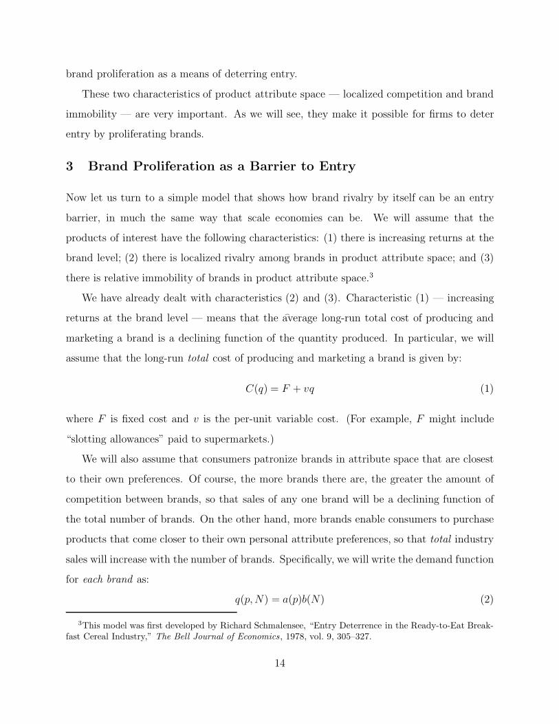
Figure 4: (a) Demand for Brand (b) Behavior of q(p, N) · N

where p is price, and N is the total number of brands. We will assume that b(N) is a

decreasing function of N , but that Nb(N) is an increasing and concave function of N . Thus,

total sales increase as N increases, but the market-expanding effect of additional brands has

decreasing returns. This is illustrated graphically in Figures 4a and 4b.

For simplicity, we will assume that all brands charge the same price p. We will also

assume that all potential entrants face a demand curve that has a sharp kink at that price

p. In other words, prices above p will not be matched, and those below p will be matched

with retaliatory price cuts. Thus, any new entrant would also charge the same price p.

Finally, the profits of a typical brand are given by:

π(p, N) = A(p)b(N) − F (3)

where A(p) = (p − v)a(p). Given p, let N∗ be the solution of π(p, N∗) = 0. All established

brands are therefore profitable as long as N < N∗. This is illustrated in Figure ??, which

shows the profit to a typical brand as a function of the total number of brands.

We will consider a very simple description of product attribute space. We will assume

that product attribute space is given by a circle with unit circumference. This is illustrated

in Figure 6. Suppose there are four brands. Where will those four brands position themselves

15

Figure 5: Profits of a Typical Brand

on the circle? Clearly they would all like to be as far away from each other as possible. Hence

the brands will be positioned as shown in the figure — each one at a distance of 1

4away

from the nearest competitor. Note that for each competitor, the local “brand density” is 4.

In other words, each competitor sees a density of four brands per unit of attribute space.

Now suppose a new entrant comes in. A new entrant would do best by locating mid-way

between two existing brands (and thereby serving those consumers least well served by the

existing brands). In the example shown in Figure 6, the new entrant would find itself at a

distance of 1

8from its nearest rival. Thus, from the point of view of this new entrant, the

local brand density is now 8, not 4.

In general, we could imagine that there are already N brands evenly distributed around

the unit circle. In that case the average brand density would be N . Suppose that N is such

that

N∗/2 < N < N∗

In this case, each of the existing brands will make a profit, because N < N∗. However,

what happens if a new entrant tries to come in? Since that entrant would face a local brand

16

Figure 6: Brand Location in Attribute Space

density of 2N , it would suffer losses. Knowing this, a rational firm would not try to enter.

We have seen here that with localized competition, entry creates a major increase in

crowding in the relevant part of attribute space, regardless of conditions (e.g., high profits)

elsewhere in the attribute space. With restricted mobility, the entrant cannot expect existing

brands to “make room” for him by changing their locations, so that the initial crowding that

entry creates will persist, and an entrant will remain unprofitable.

Note the importance of brand immobility in product attribute space. Suppose some

marketing genius could come up with a technique that would allow brands to reposition

themselves in product attribute space at low cost. Would such an invention be welcomed by

incumbent firms? You should be able to see that it would in fact threaten the profitability of

the industry. This is another example of a situation in which restricted mobility (a seeming

disadvantage) gives existing firms a competitive advantage.

17

Finally, suppose existing firms in the industry wanted to collude (implicitly or otherwise)

to deter entry. What would be the most efficient way to do so? They could threaten any

potential entrant with predatory pricing, but that might not work because once prices were

later increased, entrants would come knocking at the door again. A better scheme is simply

to increase the total number of brands. Brand proliferation can provide a natural entry

deterrent.

3.1 Nature of Inter-Firm Competition

In this model, we would expect to see only limited price competition. However, we would

expect to see very aggressive competition through advertising and new product introductions.

Furthermore, this will be a self-reinforcing process. The more effectively established brands

are differentiated through advertising, the less incentive any seller has to engage in price

competition (and recall our discussion about choosing how to compete in the context of the

beer industry.) Also, to the extent that advertising expenditures are fixed costs, they help

to deter entry. An existing brand will be kept on the market as long as its variable costs are

covered, while an entrant will only come in if it can expect to cover total costs.

Also note that aggressive advertising makes sense from what we know about the optimal

advertising-to-sales ratio. Recall that the optimal advertising-to-sales ratio is given by

A/pq = −EA/Ep

where EA is the advertising elasticity of demand, and Ep is the price elasticity of demand.4

In this case the advertising elasticity of demand is relatively high, and the price elasticity is

relatively low. Thus the advertising-to-sales ratio should be high. However, this means that

much of the extra profits from entry deterrence will be wasted away by heavy advertising,

and by the introduction of new brands. In the breakfast cereal industry, profits have still

been historically high. But imagine how much higher they would have been if firms had

somehow colluded to advertise less. Since much of this advertising is a social loss from the

4If you have forgotten this, go back and read Pindyck & Rubinfeld, Microeconomics, Chapter 11, Section

11.6.

18

point of view of consumers, the total loss to consumers from entry deterrence has been large.

3.2 Evolution of the Breakfast Cereal Industry

Table 3 shows the evolution of market shares by the major cereal producers since 1950. Note

that the acquisition of Post and Nabisco by Philip Morris, (eliminating the Nabisco brands),

and the exiting of Ralston at the end of 1993, has left four major branded companies.

Although prices and margins remain very high, the incumbent firms are facing some

important threats. Here are a couple of questions to think about.

Table 3: Volume Market Share (Percent)

1950 1960 1970 1980 1990 1993 1999 2003 2008 2011Kellogg 35.2 45.9 45.5 40.9 37.5 36.5 32.0 29.0 33.0 32.0General Mills 22.3 19.5 19.7 19.9 24.4 24.3 32.0 30.0 25.0 28.0Post* 26.8 19.6 19.3 15.6 11.1 11.9 16.0 14.5 15.0 13.0Quaker*** 5.5 3.6 7.8 8.6 7.8 7.4 9.0 13.5 7.0 7.0Malt-O-Meal 5.0 6.0Nabisco* 6.6 6.0 4.8 4.9 4.4 3.1 (Post)Ralston** 3.5 5.3 3.7 6.5 6.1 4.2Private label, Other 5.6 9.2 11.0 13.0 15.0 15.0

* Philip Morris** Exited at end of 1993*** A Subsidiary of PepsiCo, Inc.

1. During the past 15 years, there has been increased entry in the breakfast cereal market

by private labelers. What is it that in the past has made entry by an aggressive private

labeler difficult? What has changed in the last decade to allow greater entry by private

labelers?

2. Given this model of entry deterrence, how can we explain the successful entry of “nat-

ural cereals,” which were introduced by new firms during the 1970s? Sales of natural

cereals declined during the 1980s and 1990s, but have had a resurgence in recent years.

19

An example is the Kashi line of cereals (see the picture below). How do you explain

this?

Figure 7: Kashi Go Lean Cereal

20