Lecture Notes onAVL Trees

15-122: Principles of Imperative ComputationFrank Pfenning

Lecture 18March 22, 2011

1 Introduction

Binary search trees are an excellent data structure to implement associa-tive arrays, maps, sets, and similar interfaces. The main difficulty, as dis-cussed in last lecture, is that they are efficient only when they are balanced.Straightforward sequences of insertions can lead to highly unbalanced treeswith poor asymptotic complexity and unacceptable practical efficiency. Forexample, if we insert n elements with keys that are in strictly increasing ordecreasing order, the complexity will be O(n2). On the other hand, if wecan keep the height to O(log(n)), as it is for a perfectly balanced tree, thenthe commplexity is bounded by O(n ∗ log(n)).

The solution is to dynamically rebalance the search tree during insertor search operations. We have to be careful not to destroy the orderinginvariant of the tree while we rebalance. Because of the importance of bi-nary search trees, researchers have developed many different algorithmsfor keeping trees in balance, such as AVL trees, red/black trees, splay trees,or randomized binary search trees. They differ in the invariants they main-tain (in addition to the ordering invariant), and when and how the rebal-ancing is done.

In this lecture we use AVL trees, which is a simple and efficient datastructure to maintain balance, and is also the first that has been proposed.It is named after its inventors, G.M. Adelson-Velskii and E.M. Landis, whodescribed it in 1962.

LECTURE NOTES MARCH 22, 2011

AVL Trees L18.2

2 The Height Invariant

Recall the ordering invariant for binary search trees.

Ordering Invariant. At any node with key k in a binary searchtree, all keys of the elements in the left subtree are strictly lessthan k, while all keys of the elements in the right subtree arestrictly greater than k.

To describe AVL trees we need the concept of tree height, which we de-fine as the maximal length of a path from the root to a leaf. So the emptytree has height 0, the tree with one node has height 1, a balanced tree withthree nodes has height 2. If we add one more node to this last tree is willhave height 3. Alternatively, we can define it recursively by saying that theempty tree has height 0, and the height of any node is one greater than themaximal height of its two children. AVL trees maintain a height invariant(also sometimes called a balance invariant).

Height Invariant. At any node in the tree, the heights of the leftand right subtrees differs by at most 1.

As an example, consider the following binary search tree of height 3.

16

10

191 137

4height=3heightinv.sa4sfied

LECTURE NOTES MARCH 22, 2011

AVL Trees L18.3

If we insert a new element with a key of 14, the insertion algorithm forbinary search trees without rebalancing will put it to the right of 13.

height=4heightinv.sa.sfied16

10

191 137

4

14

Now the tree has height 4, and one path is longer than the others. However,it is easy to check that at each node, the height of the left and right subtreesstill differ only by one. For example, at the node with key 16, the left subtreehas height 2 and the right subtree has height 1, which still obeys our heightinvariant.

Now consider another insertion, this time of an element with key 15.This is inserted to the right of the node with key 14.

height=5heightinv.violatedat13,16,1016

10

191 137

4

14

15

LECTURE NOTES MARCH 22, 2011

AVL Trees L18.4

All is well at the node labeled 14: the left subtree has height 0 while theright subtree has height 1. However, at the node labeled 13, the left subtreehas height 0, while the right subtree has height 2, violating our invariant.Moreover, at the node with key 16, the left subtree has height 3 while theright subtree has height 1, also a difference of 2 and therefore an invariantviolation.

We therefore have to take steps to rebalance tree. We can see withouttoo much trouble, that we can restore the height invariant if we move thenode labeled 14 up and push node 13 down and to the right, resulting inthe following tree.

height=4heightinv.restoredat14,16,1016

10

191 147

4

1513

The question is how to do this in general. In order to understand this weneed a fundamental operation called a rotation, which comes in two forms,left rotation and right rotation.

3 Left and Right Rotations

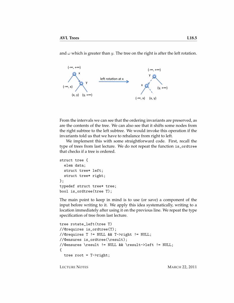
Below, we show the situation before a left rotation. We have genericallydenoted the crucial key values in question with x and y. Also, we havesummarized whole subtrees with the intervals bounding their key values.Even though we wrote −∞ and +∞, when the whole tree is a subtree of alarger tree these bounds will be generic bounds α which is smaller than x

LECTURE NOTES MARCH 22, 2011

AVL Trees L18.5

and ω which is greater than y. The tree on the right is after the left rotation.

x

y

(‐∞,+∞)

(y,+∞)

(‐∞,x)

(x,y)

y

(‐∞,+∞)

(y,+∞)

(‐∞,x) (x,y)

x

le,rota1onatx

From the intervals we can see that the ordering invariants are preserved, asare the contents of the tree. We can also see that it shifts some nodes fromthe right subtree to the left subtree. We would invoke this operation if theinvariants told us that we have to rebalance from right to left.

We implement this with some straightforward code. First, recall thetype of trees from last lecture. We do not repeat the function is_ordtreethat checks if a tree is ordered.

struct tree {elem data;struct tree* left;struct tree* right;

};typedef struct tree* tree;bool is_ordtree(tree T);

The main point to keep in mind is to use (or save) a component of theinput before writing to it. We apply this idea systematically, writing to alocation immediately after using it on the previous line. We repeat the typespecification of tree from last lecture.

tree rotate_left(tree T)//@requires is_ordtree(T);//@requires T != NULL && T->right != NULL;//@ensures is_ordtree(\result);//@ensures \result != NULL && \result->left != NULL;{

tree root = T->right;

LECTURE NOTES MARCH 22, 2011

AVL Trees L18.6

T->right = root->left;root->left = T;return root;

}

The right rotation is entirely symmetric. First in pictures:

z

y

(‐∞,+∞)

(z,+∞)

(‐∞,y) (y,z)

z

y

(‐∞,+∞)

(z,+∞)

(‐∞,y)

(y,z)

rightrota1onatz

Then in code:

tree rotate_right(tree T)//@requires is_ordtree(T);//@requires T != NULL && T->left != NULL;//@ensures is_ordtree(\result);//@ensures \result != NULL && \result->right != NULL;{

tree root = T->left;T->left = root->right;root->right = T;return root;

}

4 Searching for a Key

Searching for a key in an AVL tree is identical to searching for it in a plainbinary search tree as described in Lecture 17. The reason is that we onlyneed the ordering invariant to find the element; the height invariant is onlyrelevant for inserting an element.

LECTURE NOTES MARCH 22, 2011

AVL Trees L18.7

5 Inserting an Element

The basic recursive structure of inserting an element is the same as forsearching for an element. We compare the element’s key with the keysassociated with the nodes of the trees, inserting recursively into the left orright subtree. When we find an element with the exact key we overwritethe element in that node. If we encounter a null tree, we construct a newtree with the element to be inserted and no children and then return it. Aswe return the new subtrees (with the inserted element) towards the root,we check if we violate the height invariant. If so, we rebalance to restorethe invariant and then continue up the tree to the root.

The main cleverness of the algorithm lies in analyzing the situationswhen we have to rebalance and applying the appropriate rotations to re-store the height invariant. It turns out that one or two rotations on thewhole tree always suffice for each insert operation, which is a very elegantresult.

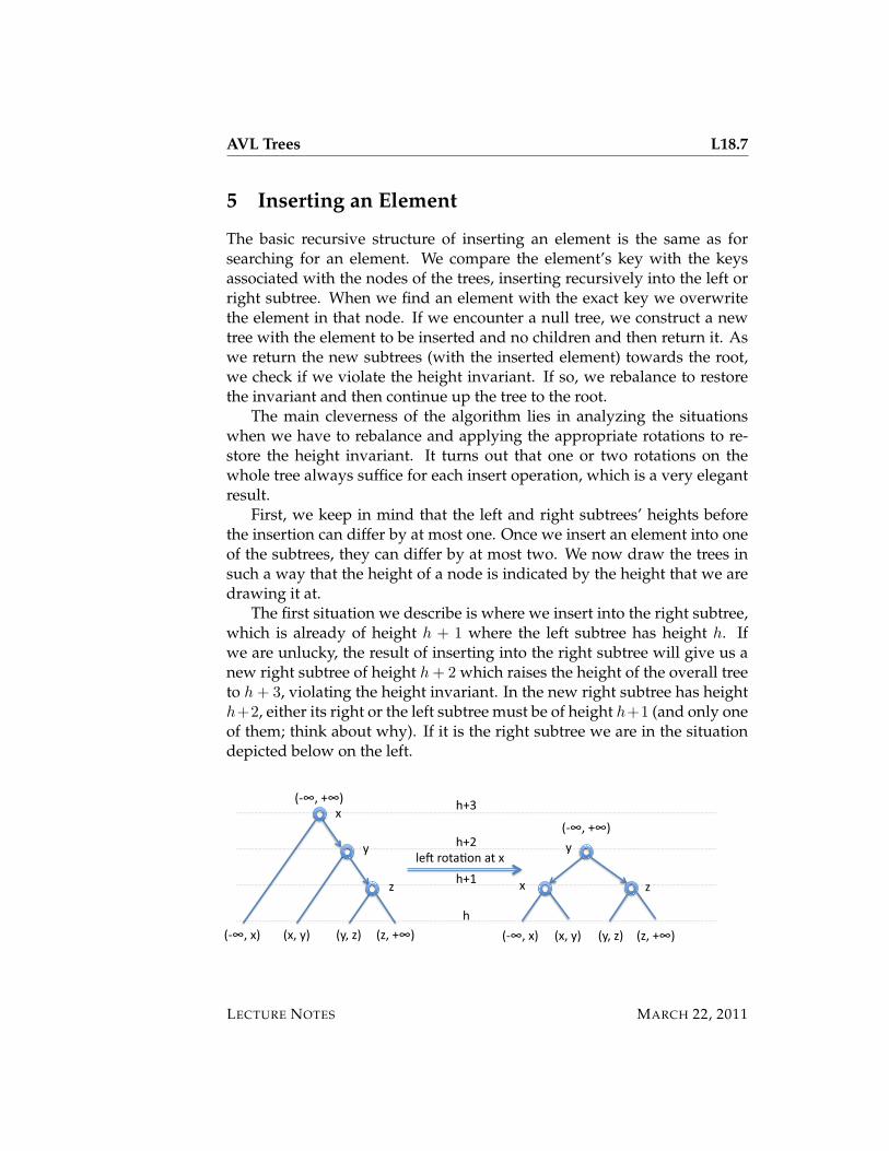
First, we keep in mind that the left and right subtrees’ heights beforethe insertion can differ by at most one. Once we insert an element into oneof the subtrees, they can differ by at most two. We now draw the trees insuch a way that the height of a node is indicated by the height that we aredrawing it at.

The first situation we describe is where we insert into the right subtree,which is already of height h + 1 where the left subtree has height h. Ifwe are unlucky, the result of inserting into the right subtree will give us anew right subtree of height h+ 2 which raises the height of the overall treeto h+ 3, violating the height invariant. In the new right subtree has heighth+2, either its right or the left subtree must be of height h+1 (and only oneof them; think about why). If it is the right subtree we are in the situationdepicted below on the left.

z

y

(‐∞,+∞)

(z,+∞)(‐∞,x) (y,z)(x,y)

x

x

y

(‐∞,+∞)

(z,+∞)(‐∞,x) (x,y) (y,z)

z

h

h+1

h+2

h+3

le1rota6onatx

LECTURE NOTES MARCH 22, 2011

AVL Trees L18.8

We fix this with a left rotation, the result of which is displayed to the right.In the second case we consider we once again insert into the right sub-

tree, but now the left subtree of the right subtree has height h+ 1.

z

y

(‐∞,+∞)

(z,+∞)(‐∞,x) (y,z)(x,y)

x

x

y

(‐∞,+∞)

(z,+∞)(‐∞,x) (x,y) (y,z)

z

h

h+1

h+2

h+3

doublerota8onatzandx

In that case, a left rotation alone will not restore the invariant (see Exer-cise 1). Instead, we apply a so-called double rotation: first a right rotation atz, then a left rotation at the root. When we do this we obtain the picture onthe right, restoring the height invariant.

There are two additional symmetric cases to consider, if we insert thenew element on the left (see Exercise 4).

We can see that in each of the possible cases where we have to restorethe invariant, the resulting tree has the same height h + 2 as before theinsertion. Therefore, the height invariant above the place where we justrestored it will be automatically satisfied.

6 Checking Invariants

The interface for the implementation is exactly the same as for binary searchtrees, as is the code for searching for a key. In various places in the algo-rithm we have to compute the height of the tree. This could be an operationof asymptotic complexityO(n), unless we store it in each node and just lookit up. So we have:

struct tree {elem data;int height;struct tree* left;struct tree* right;

};

LECTURE NOTES MARCH 22, 2011

AVL Trees L18.9

typedef struct tree* tree;

/* height(T) returns the precomputed height of T in O(1) */int height(tree T) {

return T == NULL ? 0 : T->height;}

When checking if a tree is balanced, we also check that all the heightsthat have been computed are correct.

bool is_balanced(tree T) {if (T == NULL) return true;int h = T->height;int hl = height(T->left);int hr = height(T->right);if (!(h == (hl > hr ? hl+1 : hr+1))) return false;if (hl > hr+1 || hr > hl+1) return false;return is_balanced(T->left) && is_balanced(T->right);

}

A tree is an AVL tree if it is both ordered (as defined and implementa-tion in the last lecture) and balanced.

bool is_avl(tree T) {return is_ordtree(T) && is_balanced(T);

}

We use this, for example, in a utility function that creates a new leaffrom an element (which may not be null).

tree leaf(elem e)//@requires e != NULL;//@ensures is_avl(\result);{

tree T = alloc(struct tree);T->data = e;T->height = 1;T->left = NULL;T->right = NULL;return T;

}

LECTURE NOTES MARCH 22, 2011

AVL Trees L18.10

7 Implementing Insertion

The code for inserting an element into the tree is mostly identical withthe code for plain binary search trees. The difference is that after we in-sert into the left or right subtree, we call a function rebalance_left orrebalance_right, respectively, to restore the invariant if necessary and cal-culate the new height.

tree tree_insert(tree T, elem e)//@requires is_avl(T);//@ensures is_avl(\result);{

assert(e != NULL); /* cannot insert NULL element */if (T == NULL) {T = leaf(e); /* create new leaf with data e */

} else {int r = compare(elem_key(e), elem_key(T->data));if (r < 0) {T->left = tree_insert(T->left, e);T = rebalance_left(T); /* also fixes height */

} else if (r == 0) {T->data = e;

} else { //@assert r > 0;T->right = tree_insert(T->right, e);T = rebalance_right(T); /* also fixes height */

}}return T;

}

LECTURE NOTES MARCH 22, 2011

AVL Trees L18.11

We show only the function rebalance_right; rebalance_left is sym-metric.

tree rebalance_right(tree T)//@requires T != NULL;//@requires is_avl(T->left) && is_avl(T->right);/* also requires that T->right is result of insert into T *///@ensures is_avl(\result);{

tree l = T->left;tree r = T->right;int hl = height(l);int hr = height(r);if (hr > hl+1) {//@assert hr == hl+2;if (height(r->right) > height(r->left)) {//@assert height(r->right) == hl+1;T = rotate_left(T);//@assert height(T) == hl+2;return T;

} else {//@assert height(r->left) == hl+1;/* double rotate left */T->right = rotate_right(T->right);T = rotate_left(T);//@assert height(T) == hl+2;return T;

}} else { //@assert !(hr > hl+1);fix_height(T);return T;

}}

Note that the preconditions are weaker than we would like. In partic-ular, they do not imply some of the assertions we have added in order toshow the correspondence to the pictures. This is left as the (difficult) Ex-ercise 5. Such assertions are nevertheless useful because they documentexpectations based on informal reasoning we do behind the scenes. Then,if they fail, they may be evidence for some error in our understanding, orin the code itself, which might otherwise go undetected.

LECTURE NOTES MARCH 22, 2011

AVL Trees L18.12

8 Experimental Evaluation

We would like to assess the asymptotic complexity and then experimen-tally validate it. It is easy to see that both insert and search operations taketypeO(h), where h is the height of the tree. But how is the height of the treerelated to the number of elements stored, if we use the balance invariant ofAVL trees? It turns out that h is O(log(n)). It is not difficult to prove this,but it is beyond the scope of this course.

To experimentally validate this prediction, we have to run the code withinputs of increasing size. A convenient way of doing this is to double thesize of the input and compare running times. If we insert n elements intothe tree and look them up, the running time should be bounded by c ∗ n ∗log(n) for some constant c. Assume we run it at some size n and observer = c∗n∗ log(n). If we double the input size we have c∗ (2∗n)∗ log(2∗n) =2 ∗ c ∗ n ∗ (1 + log(n)) = 2 ∗ r + 2 ∗ c ∗ n, we mainly expect the runningtime to double with an additional summand that roughly doubles with as ndoubles. In order to smooth out minor variations and get bigger numbers,we run each experiment 100 times. Here is the table with the results:

n AVL trees increase BSTs

29 0.129 − 1.018

210 0.281 2r + 0.023 2.258

211 0.620 2r + 0.058 3.094

212 1.373 2r + 0.133 7.745

213 2.980 2r + 0.234 20.443

214 6.445 2r + 0.485 27.689

215 13.785 2r + 0.895 48.242

We see in the third column, where 2r stands for the doubling of the previ-ous value, we are quite close to the predicted running time, with a approx-imately linearly increasing additional summand.

In the fourth column we have run the experiment with plain binarysearch trees which do not rebalance automatically. First of all, we see thatthey are much less efficient, and second we see that their behavior withincreasing size is difficult to predict, sometimes jumping considerably andsometimes not much at all. In order to understand this behavior, we needto know more about the order and distribution of keys that were used inthis experiment. They were strings, compared lexicographically. The keys

LECTURE NOTES MARCH 22, 2011

AVL Trees L18.13

were generated by counting integers upward and then converting them tostrings. The distribution of these keys is haphazard, but not random. Forexample, if we start counting at 0

"0" < "1" < "2" < "3" < "4" < "5" < "6" < "7" < "8" < "9"< "10" < "12" < ...

the first ten strings are in ascending order but then numbers are insertedbetween "1" and "2". This kind of haphazard distribution is typical ofmany realistic applications, and we see that binary search trees withoutrebalancing perform quite poorly and unpredictably compared with AVLtrees.

The complete code for this lecture can be found in directory 18-avl/ on thecourse website.

Exercises

Exercise 1 Show that in the situation on page 8 a single left rotation at the rootwill not necessarily restore the height invariant.

Exercise 2 Show, in pictures, that a double rotation is a composition of two ro-tations. Discuss the situation with respect to the height invariants after the firstrotation.

Exercise 3 Show that left and right rotations are inverses of each other. What canyou say about double rotations?

Exercise 4 Show the two cases that arise when inserting into the left subtreemight violate the height invariant, and show how they are repaired by a right ro-tation, or a double rotation. Which two single rotations does the double rotationconsist of in this case?

Exercise 5 Strengthen the invariants in the AVL tree implementation so that theassertions and postconditions which guarantee that rebalancing restores the heightinvariant and reduces the height of the tree follow from the preconditions.

LECTURE NOTES MARCH 22, 2011